On connection between the splitting parameters of KdV initial datum and its conservation quantities

Abstract.

An arbitrary compact-support initial datum for the Korteweg-de Vries equation asymptotically splits into solitons and a radiation tail, moving in opposite direction. We give asimple method to predict the number and amplitudes of resulting solitons and some integral characteristics of the tail using only conservation laws.

Keywords: Korteweg-de Vries equation, soliton, asymptotic, initial datum splitting.

MSC[2010]: 35Q53, 35B36.

1. Introduction

Many physical systems are modeled using equations that admit soliton solutions. Solitons and solitary waves have been observed in numerous situations and often dominate long-time behavior. The behavior of solutions of the KdV and KdV - Burgers equations is a subject of various recent research, [1]–[4]. The paper is a continuation of the previous research of the author, [5] – [10], that dealt with inhomogeneity of perturbed media.

In the case of the Korteweg-de Vries equation for an arbitrary compact-support initial datum, it eventually splits into a number of solitons plus a decaying radiation tai1 moving in opposite direction. The first numerical evidence for such a behaviour was found by Zabusky and Kruskal [11]. First rigorous results were proved by Sabat [12] and Tanaka [13]; for further history of this problem see [14]. The more recent paper [4] gives exact formulas for splitting of so called quenched solitons.

In this paper we give a simple algorithm to predict the number and amplitudes of resulting solitons and some integral characteristics of the tail. The main idea is simple enough. Since the resulting solitons and the tail are asymptotically isolated, numerically it makes sense to consider the whole solution as a sum of these solitons and tail (it is also physically reasonable). Then any conserved quantity (infinite number of them) also splits between these summands. The form of every soliton is defined by a single distinct parameter and so do its conserved quantities. This way we obtain a system of equations leading to desired estimations.

The the KdV equation considered here is of the form

$$u_{t}=2uu_{x}+u_{xxx}.$$ (1)

The solitary traveling waves (solitons) have a form of peak

$$Sol_{a,s}(x,t)=6a^{2}\mathop{\mathrm{sech}}\nolimits^{2}(a(x+s)+4a^{3}t)$$

and move to the left with velocity $4a^{2}$ and amplitude $6a^{2}$. Up to an $s$, a shift of placement on the $x$ axis, the form of a soliton is defined by the parameter $a$. Since $Sol_{a,s}(x,t)\equiv Sol_{-a,s}(x,t)$ we assume $a\geqslant 0$ below.

We use the following initial value - boundary problem for the KdV-Burgers equation on $x\in\mathbb{R}$:

$$u(x,0)=f(x),\;u(\pm\infty,t)=0,\;u_{x}(\pm\infty,t)=0.$$ (2)

We assume that the initial data $u(x,0)$ is bounded and has a compact support.

The asymptotic form (at $t\rightarrow\infty$) of the $N$-soliton solution to this problem is

$$\sum_{i=1}^{N}6a_{i}^{2}\mathop{\mathrm{sech}}\nolimits^{2}(a_{i}x+p_{i}+4a_{i}^{3}t)+R(x,t),$$

where $R(x,t)$ is a tail and phase shifts are given by the formula

$$p_{i}=\frac{1}{2}\log\left(\frac{\gamma_{i}}{2a_{i}}\cdot\prod_{j=i+1}^{N}\left(\frac{a_{j}-a_{i}}{a_{j}+a_{i}}\right)^{2}\right).$$

Here $\{-a^{2}_{i}\}$ is the the discrete specter of the differential operator $-\frac{d^{2}}{dx^{2}}-f(x)$ and $\gamma_{i}$ are the norming constants from the inverse scattering procedure. For an arbitrary $f(x)$ this data is hard to obtain, so estimations, proposed in this paper and based solely on conserved quantities may be useful.

For numerical computations we use $x\in[a,b]$ for appropriately large $a,\;b$ instead of $\mathbb{R}$.

2. Conservation laws

2.1. Soliton’s accompanying series

The first four conserved quantities for KdV are

$$I_{1}(u)) = \int_{-\infty}^{+\infty}u(x,t)\,dx\mbox{ --- mass,}$$

$$I_{2}(u) = \int_{-\infty}^{+\infty}u^{2}(x,t)\,dx\mbox{ --- momentum,}$$

$$I_{3}(u) = \int_{-\infty}^{+\infty}\left(2u^{3}(x,t)-3(u_{x}(x,t))^{2}\right)\,dx\mbox{ --- energy,}$$

$$I_{4}(u) = \int_{-\infty}^{+\infty}\left(5u^{4}(x,t)-30u(x,t)(u_{x}(x,t))^{2}+9(u_{xx}(x,t))^{2}\right)\,dx,$$

and there are infinite number of them.

There is a simple recurrent procedure to generate $I_{k}(u)\rightarrow I_{k+1}(u)$ using the bi-hamiltonian structure of KdV (see [14]); note that for the KdV of the form $u_{t}=u_{xxx}+2uu_{x}$ the hamiltonian operators are $D$ and $(D^{3}+uD+u_{x})$, where $D$ is a total derivative with respect to $x$.

If $u(x,t)$ is a solution of KdV then $\dfrac{\partial}{\partial t}I_{k}(u)=0$. So if $u(x,t)$ is the solution with the initial value $u(x,0)=f(x)$ then $I_{k}(u)=I_{k}(f)$. Thus $I_{k}(f)$ is conserved in time

In particular, for solitons
$u(x,t)=Sol_{a,s}(x,t)=6a^{2}\mathop{\mathrm{sech}}\nolimits^{2}(a(x+s)+4a^{3}t)$ we have

$$I_{1}(Sol_{a,s}) = \int_{-\infty}^{+\infty}6a^{2}\mathop{\mathrm{sech}}\nolimits^{2}(ax)\,dx=12a,$$ (3)

$$I_{2}(Sol_{a,s}) = \int_{-\infty}^{+\infty}(6a^{2}\mathop{\mathrm{sech}}\nolimits^{2}(ax))^{2}\,dx=48a^{3},$$

$$I_{3}(Sol_{a,s}) = \frac{1728}{5}a^{5},$$

$$I_{4}(Sol_{a,s}) = \frac{20736}{7}a^{7},$$

$$\dots \dots \dots$$

$$I_{l}(Sol_{a,s}) = K_{l}a^{2l-1}.$$

We obtained the series, common for all KdV solitons, in odd powers of the parameter $a$.

2.2. Predicting the final pattern of evolution

If $q(x)=u(x,0)$ is an arbitrary initial datum with compact support (it is also called a potential), it eventually splits into a number of solitons plus a decaying radiation tail moving in opposite direction. A potential without a tail is called reflectionless.

2.2.1. Reflectionless splitting

Since after some deliberation $q(x)$ splits (at least numerically) into a disconnected sum of $N$ different-speed solitons, we get

$$I_{1}(q)) = \int_{-\infty}^{+\infty}q(x)\,dx=\sum_{i=1}^{N}\int_{-\infty}^{+\infty}Sol_{a_{i},s}\,dx=12\sum_{i=1}^{N}a_{i}$$

$$I_{2}(q) = \int_{-\infty}^{+\infty}q^{2}(x)\,dx=48\sum_{i=1}^{N}a_{i}^{3}$$

$$I_{3}(q) = \int_{-\infty}^{+\infty}\left(2q^{3}(x)-3(q_{x}(x))^{2}\right)\,dx=\frac{1728}{5}\sum_{i=1}^{N}a_{i}^{5}$$

$$I_{4}(q) = \int_{-\infty}^{+\infty}\left(5q^{4}(x)-30q(x)(q_{x}(x))^{2}+9q_{xx}(x)^{2}\right)\,dx=\frac{20736}{7}\sum_{i=1}^{N}a_{i}^{7}$$

$$\dots \dots$$

Thus we obtain the system to obtain $a_{i},\;i=1\dots N:$

$$K_{j}\sum_{i=1}^{N}a_{i}^{2j+1}=I_{j}(q),\;j=1\dots N,$$

where $K_{j}$ is the constant specific to the $j$-th conserved quantity and $a_{1}\geqslant a_{1}>a_{2}>\dots a_{N}>0$ is assumed.

Of course, the above equation hold for all $j=1\dots\infty$, but to find $N$ solitons it suffice to consider only first $N$ equations.

2.2.2. General case

If a reflection is present then the reflected tail eventually disconnects from solitons and (2.2.1) holds no more. Instead, we get

$$I_{1}(q)) = 12\sum_{i=1}^{N}a_{i}+\int_{-\infty}^{+\infty}R(x,t)\,dx$$

$$I_{2}(q) = 48\sum_{i=1}^{N}a_{i}^{3}+\int_{-\infty}^{+\infty}R^{2}(x,t)\,dx$$

$$I_{3}(q) = \frac{1728}{5}\sum_{i=1}^{N}a_{i}^{5}+\int_{-\infty}^{+\infty}\left(2R^{3}(x,t)-3(R_{x}(x,t))^{2}\right)\,dx$$

$$\dots \dots$$

It follows that the discrepancies $I_{j}(R(x,t))=I_{j}(q)-K_{j}\sum_{i=1}^{N}a_{i}^{2j+1}$ are also constant.

The first four of $I_{j}(R)$ are alternating in sign. Indeed, at least the initial perturbation mass is carried away by solitons, so $I_{1}(R)\leqslant 0$; Since momentum of any part of solution is non-negative, it follows that $I_{2}(R)\geqslant 0$. The reflected tail is oscillating around zero value, therefore

$$\int_{-\infty}^{+\infty}\left(2R^{3}(x,t)\right)\,dx\mbox{ is small while }\int_{-\infty}^{+\infty}\left(-3(R_{x}(x,t))^{2}\right)\,dx$$

is negative and comparatively large; so $I_{3}(R)\leqslant 0$. Similarly plausible argument can be applied to $I_{4}(R)$ if the conservation law is rewritten to equivalent quadratic form

$$5u^{4}-30uu_{x}^{2}+9u_{xx}^{2}\sim 5u^{4}+15u^{2}u_{xx}+9u_{xx}^{2}=9(u^{2}+\frac{5+\sqrt{5}}{6}u_{xx})(u^{2}+\frac{5-\sqrt{5}}{6}u_{xx});$$

the rigorous proof of alternation in the case of a tail will be published elsewhere.

Hence we obtain the system of necessary conditions

$$I_{1}(q) \leqslant 12\sum_{i=1}^{N}a_{i}$$

$$I_{2}(q) \geqslant 48\sum_{i=1}^{N}a_{i}^{3}$$

$$I_{3}(q) \leqslant \frac{1728}{5}\sum_{i=1}^{N}a_{i}^{5}$$

$$I_{4}(q) \geqslant \frac{20736}{7}\sum_{i=1}^{N}a_{i}^{7}$$

$$\dots \dots;$$

$$a_{i} \geqslant 0.$$

The system is very simple and can be effectively used in predicting the number of solitons and their parameters in the resulting splitting. For one, a solution of (2.2.1) is a rough approximation to the splitting parameters.

2.2.3. Number of solitons.

The system (2.2.2) defines the admissible domain in $\{x_{1},x_{2},\dots,x_{n}\}$, the solitons’parameters space. In order for this domain not to be empty a number of inequalities must hold, for instance $I_{1}(q)\leqslant 12\sum_{i=1}^{N}a_{i},\;I_{2}(q)\geqslant 48\sum_{i=1}^{N}a_{i}^{3}$. In the case $n=2$ we get $a_{1}+a_{2}\geqslant p_{1},\;a_{1}^{3}+a_{2}^{3}\leqslant p_{3}$ (here $p_{k}=K^{-1}_{j}I_{j}(q)$, $j=2k-1$).

The admissible domain would be nonempty if $OA>OB$ as on the graph 1 (left), where $p_{1}=1,p_{2}=0.5$. For both points $A$ and $B$ $a_{1}=a_{2}$, so $OA=\sqrt{2\left(\frac{p_{1}}{2}\right)^{2}}=\sqrt{\frac{1}{2}}$ and $OB=\sqrt{2\left(\frac{p_{2}}{2}\right)^{2}}=\sqrt{\frac{1}{8}}$

But in the case shown on the right part of the figure $p_{1}=1,p_{2}=0.2$ the admissible domain is empty. Let’s increase the number of solitons to $n$. Then $a_{1}=a_{2}=\dots a_{n}=\frac{1}{n}$ for $A$ and $a^{3}_{1}=a^{3}_{2}=\dots=a^{3}_{n}=\frac{0.2}{n}$. Thus if we require $OA^{2}=n\left(\frac{1}{n^{2}}\right)\geqslant OB^{2}=n\left(\sqrt[3]{\frac{0.2}{n}}\right)^{2}\Rightarrow n^{2}>5\Rightarrow n=3.$

For arbitrary $p_{1},p_{2}$ the smallest number of solitons is the integer $n$ such that

$$n\geqslant\sqrt{\frac{p_{1}^{3}}{p_{2}}}.$$ (4)

For other conserved quantities similar conditions of non-emptiness of the admissible domain lead to compare $n^{k-1}\vee\frac{p_{1}^{k}}{p_{2}}$. However usually (eg,for all examples below) it suffice to use (4) to predict the right number of resulting solitons

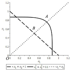
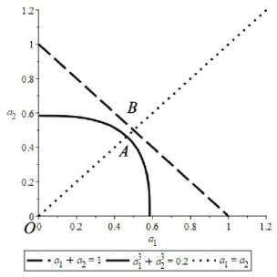
Figure 1. Defining the number of solitons.
Left: $n=2$. Right: $n=3$

3. Examples

3.1. 1-soliton $q(x)=1+\cos(x),\mbox{ on }x\in[-\pi,\pi]$

In this example $I_{1}(q)=2\pi,\;I_{2}(q)=3\pi,\;I_{3}(q)=7\pi$.

The number of solitons $n>\sqrt{\frac{p_{1}^{3}}{p_{2}}}=\sqrt{\left(\frac{\pi}{6}\right)^{3}/\frac{\pi}{16}}\thickapprox 0.48\Rightarrow n=1$

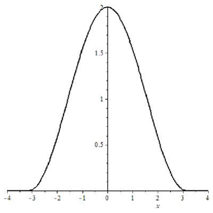
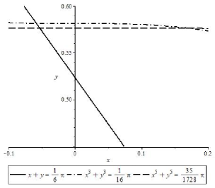
Figure 2. Left: Initial perturbation $q(x)=1+\cos(x)$; $t=0$. Right: Admissible domain is bounded by dash, dash-dot lines and $y$ axis.

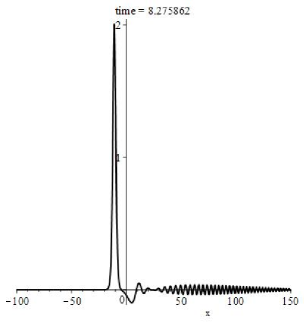
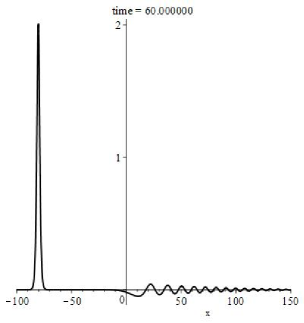
Figure 3. Splitting of the initial perturbation
$q(x)=1+\cos(x),\mbox{ on }x\in[-\pi,\pi]$, Left: $t=8$. Right: $t=60$.

The amplitude of the resulting soliton can be measured wih high precision. It is $2.005=6a_{1}^{2}$ , see figure 3, so $a_{1}\approx 0.578$. The inequalities

$$I_{1}(q)=2\pi\leqslant 12a_{1},\;I_{2}(q)=3\pi\geqslant 48a_{1}^{3},\;I_{3}(q)=7\pi\leqslant\frac{1728}{5}a_{1}^{5}$$

hold:

$$\frac{\pi}{6}\approx 0.524<\sqrt[5]{\frac{35\pi}{1728}}\approx 0.576<a_{1}<\sqrt[3]{\frac{\pi}{16}}\approx 0.581.$$

The system $a_{1}+a_{2}=\frac{\pi}{6},];a_{1}^{3}+a_{2}^{3}=\frac{\pi}{16}$ does admit non-positive solution $(0.581,-0.058)$, and $a_{1}\approx 0.578,a_{2}=0$ is an admissible point, nearest to it, see figure (2).

Also note that we obtained the conserved quantities for the radiation tail. They are discrepancies $\{I_{l}(R)=I_{l}(q)-K_{l}\sum_{i=1}^{n}a_{i}^{2l-1}\}$. In particular, in this example $l=n=1$, $K_{1}=12$ and the mass of the tail is $I_{1}(R)=2\pi-12\cdot 0.578=-0.065$

3.2. 2-soliton $q(x)=4(1+\cos(x)),\mbox{ on }x\in[-\pi,\pi]$

In this example $I_{1}(q)=8\pi,\;I_{2}(q)=48\pi,\;I_{3}(q)=592\pi$, see figure 4.

The number of solitons $n>\sqrt{\frac{p_{1}^{3}}{p_{2}}}=\sqrt{\pi^{3}/\frac{2\pi}{3}}\thickapprox 1.7\Rightarrow n=2$

The corresponding system for 2-soliton is $a_{1}+a_{2}=\frac{2\pi}{3},];a_{1}^{3}+a_{2}^{3}=\pi$ has a solution $a_{1}=1.414,a_{2}=.681$, while system on 3-solitons has no positive solutions.

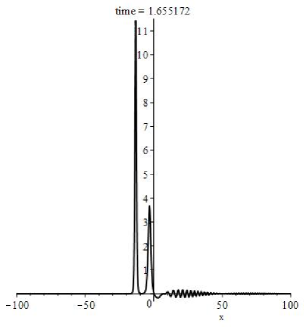
Figure 4. Splitting of the initial perturbation
$q(x)=4(1+\cos(x)),\mbox{ on }x\in[-\pi,\pi]$, Left: $t=1.7$. Right: $t=12$.

The amplitudes of the resulting two solitons measure $11.51=6a_{1}^{2}$, $3.65=6a_{2}^{2}$, so $a_{1}\approx 1.385$ and $a_{2}\approx 0.780$. The inequalities hold:

$$\frac{2\pi}{3}\approx 2.094<a_{1}+a_{2}\approx 2.165;$$

$$a_{1}^{3}+a_{2}^{3}\approx 3.131<\pi\approx 3.142.$$

$$\frac{5\cdot 592\pi}{1728}\approx 5.381<a_{1}^{5}+a_{2}^{5}\approx 5.383.$$

3.3. 3-soliton $q(x)=8(1+\cos(x)),\mbox{ on }x\in[-\pi,\pi]$

In this example $I_{1}(q)=16\pi,\;I_{2}(q)=192\pi,\;I_{3}(q)=4928\pi$, see figure 5.

The number of solitons $n>\sqrt{\frac{p_{1}^{3}}{p_{2}}}=\sqrt{\frac{4\pi^{3}}{3}/\frac{4\pi}{3}}\thickapprox 2.4\Rightarrow n=3$

The corresponding system for 3-soliton is $a_{1}+a_{2}+a_{3}=\frac{4\pi}{3},];a_{1}^{3}+a_{2}^{3}+a_{3}^{3}=4\pi,\;$ $a_{1}^{5}+a_{2}^{5}+a_{3}^{5}=\frac{5\cdot 4928\pi}{1728}$ has a solution $a_{1}=2.034,a_{2}=1.583,a_{3}=0.572$.

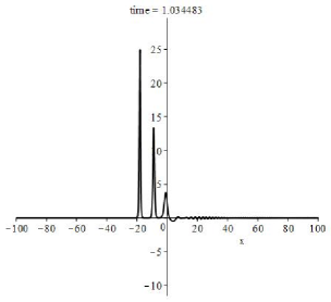
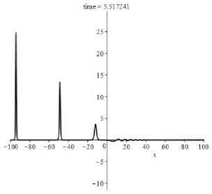
Figure 5. Splitting of the initial perturbation
$q(x)=8(1+\cos(x)),\mbox{ on }x\in[-\pi,\pi]$, Left: $t=1$. Right: $t=5.5$.

The amplitudes of the resulting solitons measure $25.5=6a_{1}^{2}$, $13.4=6a_{2}^{2}$, $3.7=6a_{3}^{2}$, so $a_{1}\approx 2.062$, $a_{2}\approx 1.492$ and $a_{3}\approx 0.780$. The inequalities hold:

$$\frac{4\pi}{3}\approx 4.189<a_{1}+a_{2}+a_{3}\approx 4.333;$$

$$\frac{5\cdot 4928\pi}{1728}\approx 44.797<a_{1}^{5}+a_{2}^{5}+a_{3}^{5}\approx 44.9100;$$

$$a_{1}^{3}+a_{2}^{3}+a_{3}^{3}\approx 12.555<4\pi\approx 12.567.$$

3.4. 5-soliton $q(x)=0.4(-\tanh(x-15)+\tanh(x+15))$

In this example $I_{1}(q)=24\;I_{2}(q)=18.56,\;I_{3}(q)=27.904,\;I_{4}(q)=55.637$, see figures 6, 7

The number of solitons $n>\sqrt{\frac{p_{1}^{3}}{p_{2}}}=\sqrt{\frac{2^{3}}{0.3867}}\thickapprox 4.5\Rightarrow n=5$

The corresponding system for 4-solitons, $\sum_{i=1}^{4}a_{i}^{2j-1},\;j=1,\dots,4$ has no solutions.

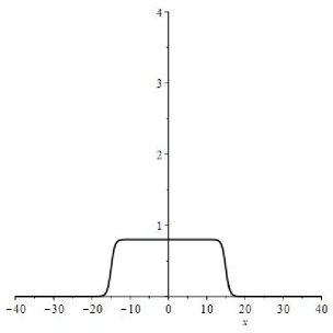
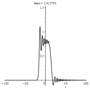
Figure 6. Left: Initial perturbation $q(x)=0.4(-\tanh(x-15)+\tanh(x+15))$. Right: Splitting begins as a shock wave,$t=2.4$.

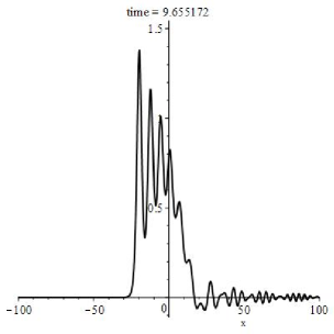
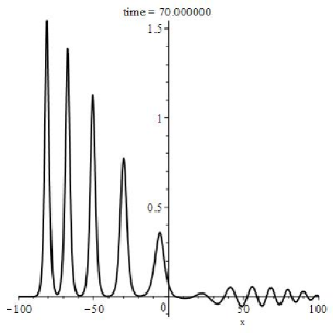
Figure 7. Splitting of the initial perturbation
$q(x)=0.4(-\tanh(x-15)+\tanh(x+15))$, Left: $t=9.7$. Right: $t=70$.

The amplitudes of the resulting five solitons measure $1.543=6a_{1}^{2}$, $1.385=6a_{2}^{2}$, $1.125=6a_{3}^{2}$, $0.775=6a_{4}^{2}$, $0.36=6a_{5}^{2}$, so $a_{1}\approx 0.507$, $a_{2}\approx 0.480$, $a_{3}\approx 0.433$, $a_{4}\approx 0.359$, $a_{2}\approx 0.245$. The inequalities hold:

$$K_{j}\sum_{i=1}^{5}a_{i}^{2j-1}\geqslant I_{j}(q)\mbox{ for }j=1,3\mbox{ and }K_{j}\sum_{i=1}^{5}a_{i}^{2j-1}\leqslant I_{j}(q)\mbox{ for }j=2,4$$

3.5. 2-soliton $q(x)=1+\cos(2x),\mbox{ on }x\in[-\pi/2,3\pi/2]$

In this example $I_{1}(q)=2\pi,\;I_{2}(q)=3\pi,\;I_{3}(q)=-2\pi$, see figure 9. Note that mass and momentum coincide with those in the first example, so $n>1$. But in contrast to the example 1, $n=2$ since admissible domain is much larger in this case: the third inequality produce no restrictions in positive domain, see figure 8.

The corresponding system for 3-solitons, $a_{1}+a_{2}+a_{3}=\frac{\pi}{6},\;a_{1}^{3}+a_{2}^{3}+a_{3}^{3}=\frac{\pi}{16},$ $a_{1}^{5}+a_{2}^{5}+a_{3}^{5}=-\frac{10\pi}{1728}$, has no solutions.

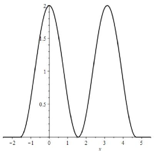
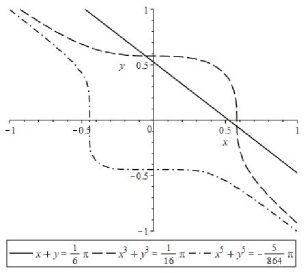
Figure 8. Left: Initial perturbation $q(x)=1+\cos(2x)$; $t=0$. Right: Admissible domain is bounded by dash, solid lines and $y$ axis.

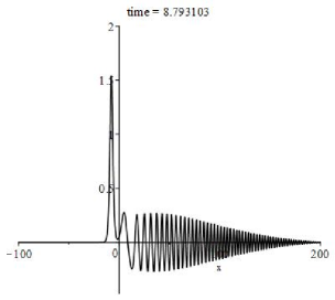
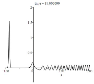
Figure 9. Splitting of the initial perturbation
$q(x)=1+\cos(2x),\mbox{ on }x\in[-\pi/2,3\pi/2]$, Left: $t=8.8$. Right: $t=85$.

The amplitudes of the resulting solitons measure $1.55=6a_{1}^{2}$, $0.175=6a_{2}^{2}$, so $a_{1}\approx 0.508$, $a_{2}\approx 0.1731$. The inequalities hold:

$$\sqrt[5]{\frac{-10\pi}{1728}}<\frac{\pi}{6}<a_{1}+a_{2}$$

$$a_{1}^{3}+a_{2}^{3}\thickapprox 0.136<\frac{\pi}{16}$$

The 2-soliton system $a_{1}+a_{2}=\frac{\pi}{6},\;a_{1}^{3}+a_{2}^{3}=\frac{\pi}{16}$ does admit non-positive solution $(0.581,-0.058)$, and $a_{1},a_{2}$ is the admissible point, not far from this solution, see figure 8.

Remark. It must be noted here that the described method is not as effective when the initial data consists of a disjoint union of perturbations. Later generated solitons in this case collide with tails of previous solitons and a whole picture becomes tangled, at least for a initial short period.

Conclusion

The present paper as well as our previous research of the KdV solitons in nonhomogeneous media ([5]–[10]) persuades that a distorted by inhomogeneity compact impulse getting into homogeneous region behaves according the same scenario: it became a soliton or splits into two or more. Usually, but not necessarily, the obstacle generates a reflected wave. This effect has the same nature as the splitting of the initial compact perturbation (or potential) into solitons and a radiation tail in the case of the classical KdV; the number and parameters of resulting solitons vary, but the scenario stays invariable.

We connected the number, amplitudes and velocities of a train of solitons that is result of a splitting of an arbitrary initial compact datum for the KdV with its conservation laws; some rough estimations are exemplified above.

A form of a transformed wave, its reflection and refraction coefficients may be easily predicted. Thus the possibility of control of solitary impulses arises. So the results may be of a practical use.

The figures in this paper were generated numerically using Maple PDETools package. The mode of operation uses the default Euler method, which is a centered implicit scheme, and can be used to find solutions to PDEs that are first order in time, and arbitrary order in space, with no mixed partial derivatives.

Acknolegement

This work was partially supported by the Russian Basic Research Foundation grant 18-29-10013.

References

- [1] Grunert K., Teschl G., Long–Time Asymptotics for the Korteweg–de Vries Equation via Nonlinear Steepest Descent, Mathematical Physics, Analysis and Geometry volume 12, pages 287–324 (2009)
- [2] Khruslov E. Ya., Stephan H., Splitting of some non–localized solutions of the Korteweg–de Vries equation into solitons, Mat. Fiz. Anal. Geom., 1998, Volume 5, Number 1/2, 49–67
- [3] Grava T., Whitham modulation equations and application to small dispersion asymptotics and long time asymptotics of nonlinear dispersive equations arXiv:1701.00069v1 [math-ph] 31 Dec 2016
- [4] Gamayun O., Semenyakin M., Soliton splitting in quenched classical integrable systems. arXiv:1512.02035v1 [cond-mat.quant-gas] 7 Dec 2015
- [5] Samokhin A.V., Soliton transmutations in KdV—Burgers layered media, Journal of Geometry and Physics, Volume 148, February 2020, 9 pages, 103547. Available online 14 November 2019. https://doi.org/10.1016/j.geomphys.2019.103547
- [6] Samokhin A.V., Reflection and refraction of solitons by the KdV–Burgers equation in nonhomogeneous dissipative media, Theoretical and Mathematical Physics, 197(1): 1527–1533 (2018) DOI: 10.1134/S0040577918100094
- [7] Samokhin A., Nonlinear waves in layered media: solutions of the KdV — Burgers equation. Journal of Geometry and Physics 130 (2018) pp. 33–39 https://doi.org/10.1016/j.geomphys.2018.03.016
- [8] Samokhin A., On nonlinear superposition of the KdV-Burgers shock waves and the behavior of solitons in a layered medium. Journal of Differential Geometry and its Applications. 54, Part A, October 2017, pp 91–99. https://doi.org/10.1016/j.difgeo.2017.03.001
-
[9]
Samokhin A., Periodic boundary conditions for KdV-Burgers equation on an interval. Journal of Geometry and Physics 113 (2017), pp. 250–256
http://dx.doi.org/10.1016/j.geomphys.2016.07.006 - [10] Samokhin A.V., The KdV soliton crosses a dissipative and dispersive border. arXiv:2002.00432 [nlin.SI], 11 pages
- [11] Zabusky N.J. and Kruskal M.D., Interaction of solitons in a collisionless plasma and the recurrence of initial states, Phys. Rev. Lett. 15, 240–243 (1965).
- [12] Shabat A.B., On the Korteweg-de Vries equation, Soviet Math. Dokl. 14, 1266–1270 (1973).
- [13] Tanaka S., Korteweg-de Vries equation; Asymptotic behavior of solutions, Publ. Res. Inst. Math. Sci. 10, 367–379 (1975).
- [14] : Krasil’shchik I.S., Vinogradov A.M. et al. Symmetries and Conservation Laws for Differential Equations of Mathematical Physics, Providence RI: American Mathematical Society, 335 pp.