A Newton multigrid framework for optimal control of fluid-structure interactions

Abstract

In this paper we consider optimal control of nonlinear time-dependent fluid structure interactions. To determine a time-dependent control variable a BFGS algorithm is used, whereby gradient information is computed via a dual problem. To solve the resulting ill conditioned linear problems occurring in every time step of state and dual equation, we develop a highly efficient monolithic solver that is based on an approximated Newton scheme for the primal equation and a preconditioned Richardson iteration for the dual problem. The performance of the presented algorithms is tested for one 2d and one 3d example numerically.

Keywords: fluid-structure interactions; finite elements; multigrid; optimal control; parameter estimation

1 Introduction

Fluid-structure interactions are part of various applications ranging from classical engineering problems like aeroelasticity or naval design to medical applications, e.g. the flow of blood in the heart or in blood vessels. More and more of these applications are regarded recently in combination with optimal control, shape-optimization, and parameter estimation. Especially in hemodynamical applications — in order to get a deeper understanding of the development of vascular diseases — patient specific properties have to be incorporated into the models. For example, in [8, 9, 10, 15, 28, 34, 32] patient specific boundary conditions and vessel material parameters are determined to simulate arterial blood flow. Similar approaches using gradient information have been proposed in  [15, 7, 35] to estimate Young’s modulus of an artery.

As computer tomography (CT) and magnetic resonance imaging (MRI) evolve rapidly, already very accurate measurements of the movement of the vessel wall are possible nowadays and even averaged flow profiles in blood vessels can be provided, see [1, 8, 27]. To incorporate the data in the vascular models, it is necessary to improve the available parameter estimation and optimal control algorithms for fluid-structure interaction applications, in particular since only few approaches in the literature take the sensitivity information of the full time-dependent nonlinear system into account. For example in [14, 29], adjoint equations are derived for one-dimensional fluid-structure interaction configurations and in [41] for a stationary fluid-structure interaction problem. In contrast, the authors of [34, 10, 32, 8] use a sequential reduced Kalman filter. Peregio, Veneziani, and Vergara [35] compute sensitivity information to estimate the wall stiffness. To reduce the computational time, they solve in every time-point an optimal control problem. As the mesh motion is discretized via an explicit time-stepping scheme, no sensitivity information of the mesh motion equation has to be computed. Similar to the articles [10, 8, 32], the estimated parameters are updated in every time step and the forward simulation only runs once.

In this paper we are going to compute gradient information for the full time-dependent nonlinear system for 3d applications. Thereby, the optimization algorithm takes the intrinsic property of fluid-structure interaction, transport over time, into account. In addition the here presented approach enables to regard tracking type functionals with observation at a singular time-point or on a specific time-interval. Furthermore a time-dependent parameter can be reconstructed. This would not be possible, if we would use a Kalman filter or would solve an optimization problem in every time step as in the literature cited above. The dual problem to compute sensitivities can be derived as in [17] or as in [20], where sensitivity information was used for a dual-weighted residual error estimator.

For various applications and a general overview on modeling and discretization techniques for fluid-structure interactions we refer to the literature [3, 39]. Mathematically, two challenges come together in fluid-structure interactions: First, fluid-structure interactions are free boundary value problems. The governing domains for the fluid - we will consider the incompressible Navier-Stokes equations - and the solid - we consider hyperelastic materials like the St. Venant Kirchhoff model - move and the motion is determined by the coupled dynamics, i.e. it is not known a priori. This geometric problem is treated by mapping onto a fixed domain [16] such that movement of the boundary is incorporated into the equation and we can derive the dual problem on the fixed reference domain. Second, the two problems that are coupled are of different type, the parabolic Navier-Stokes equation and the hyperbolic solid problem. On the common and moving interface, both systems are coupled by different conditions. This coupling gives rise to stability problems that can call for small time steps or many subiterations. Most prominently this problem shows itself in the so called added mass effect [13]. The added mass effect is of particular relevance in hemodynamical applications, that are focus of this work [26], and calls for monolithic formulations and strongly coupled discretizations and solution techniques. This property is transmitted to the dual problem, such that we have to derive strongly coupled solution techniques for the dual problem. To compute dual information, we extend the Newton solver proposed for time-dependent fluid-structure interactions in [19] to the dual problem. Thereby, iterative solvers, preconditioned with geometric multigrid, can solve the resulting linear problems in every state and dual time step very robust and efficiently.

In Section 2 we present the optimal control problem, which is discretized in Section 3 in space and time. For the discretized system we derive optimality conditions. In Section 4 we discuss modifications for the Newton scheme presented first in [19] and extend the approach to the dual problem. Finally we test the proposed algorithm in Section 5 numerically to analyze the behavior of the Newton scheme. In addition we take a closer look on the convergence behavior of the iterative solvers.

2 Governing equations

Here, we present the optimal control problem of a tracking type functional subject to fluid structure interactions. We use a monolithic formulation for the fluid-structure interaction model coupling the incompressible Navier-Stokes equations and an hyperelastic solid, based on the St. Venant Kirchhoff material. For details we refer to [39]. The here presented optimization approach can be directly extended to specific material laws used in hemodynamics. As control variable we chose exemplarily the mean pressure over time at the outflow boundary. In the following we restrict us to the control space $Q=L^{2}(I)$, but the here presented optimization algorithm can as well be applied to determine material parameters (e.g. $Q=\mathds{R}^{n}$) or space-distributed parameters (e.g. $Q=L^{2}(\Omega)$) entering the fluid- or solid-problem.

On the $d$-dimensional domain, partitioned in reference configuration $\Omega=\mathcal{F}\cup\mathcal{I}\cup\mathcal{S}$, where $\mathcal{F}$ is the fluid domain, $\mathcal{S}$ the solid domain and $\mathcal{I}$ the fluid structure interface, we denote by $\mathbf{v}$ the velocity field, split into fluid velocity $\mathbf{v}_{f}:=\mathbf{v}|_{\mathcal{F}}$ and solid velocity $\mathbf{v}_{s}:=\mathbf{v}|_{\mathcal{S}}$, and by $\mathbf{u}$ the deformation field, again with $\mathbf{u}_{s}:=\mathbf{u}|_{\mathcal{S}}$ and $\mathbf{u}_{f}:=\mathbf{u}|_{\mathcal{F}}$. The boundary of the fluid domain $\Gamma_{f}:=\partial\mathcal{F}\setminus\mathcal{I}$ is split into inflow boundary $\Gamma_{f}^{in}$ and wall boundary $\Gamma_{f}^{wall}$, where we usually assume Dirichlet conditions, $\Gamma_{f}^{D}:=\Gamma_{f}^{in}\cup\Gamma_{f}^{wall}$, and a possible outflow boundary $\Gamma_{f}^{out}$, where we enforce the do-nothing outflow condition [24], and the control boundary $\Gamma_{q}$. The solid boundary $\Gamma_{s}=\partial\mathcal{S}\setminus\mathcal{I}$ is split into Dirichlet part $\Gamma_{s}^{D}$ and a Neumann part $\Gamma_{s}^{N}$.

We formulate the coupled fluid-structure interaction problem in a strictly monolithic scheme by mapping the moving fluid domain onto the reference state via the ALE map $T_{f}(t):\mathcal{F}\to\mathcal{F}(t)$, constructed by a fluid domain deformation $T_{f}(t)=\operatorname{id}+\mathbf{u}_{f}(t)$. In the solid domain, this map $T_{s}(t)=\operatorname{id}+\mathbf{u}_{s}(t)$ denotes the Lagrange-Euler mapping and as the deformation field $\mathbf{u}$ will be defined globally on $\Omega$ we simply use the notation $T(t)=\operatorname{id}+\mathbf{u}(t)$ with the deformation gradient $\mathbf{F}:=\nabla T$ and its determinant $J:=\operatorname{det}(\mathbf{F})$.

For given desired states $\tilde{\mathbf{v}}(t)\in L^{2}(\mathcal{F})$ or $\tilde{\mathbf{u}}(t)\in L^{2}(\mathcal{S})$, we find the global (in fluid and solid domain) velocity and deformation fields

$$\mathbf{v}(t) \in\mathbf{v}^{D}(t)+H^{1}_{0}(\Omega;\Gamma_{f}^{D}\cup\Gamma_{s}^{D})^{d}\text{ and }\mathbf{u}(t)\in\mathbf{u}^{D}(t)+H^{1}_{0}(\Omega;(\partial\mathcal{F}\setminus\mathcal{I})\cup\Gamma_{s}^{D})^{d},$$

the pressure $p\in L^{2}(\mathcal{F})$ and the control parameter $q\in Q$ satisfying the initial condition $\mathbf{v}(0)=\mathbf{v}_{0}$ and $\mathbf{u}(0)=\mathbf{u}_{0}$, as solution to

$$\min_{q\in Q}J(q,\mathbf{v},\mathbf{u})=\frac{1}{2}\int_{I}\lVert\mathbf{v}-\tilde{\mathbf{v}}\rVert^{2}_{\mathcal{F}}\text{ d}t+\frac{1}{2}\int_{I}\lVert\mathbf{u}-\tilde{\mathbf{u}}\rVert^{2}_{\mathcal{S}}\text{ d}t+\frac{\alpha}{2}\lVert q\rVert^{2}_{Q}$$ (1)

and subject to

$$\big{(}J(\partial_{t}\mathbf{v}+(\mathbf{F}^{-1}(\mathbf{v}-\partial_{t}\mathbf{u})\cdot\nabla)\mathbf{v},\phi\big{)}_{\mathcal{F}}+\big{(}J\boldsymbol{\sigma}_{f}\mathbf{F}^{-T},\nabla\phi\big{)}_{\mathcal{F}}$$ (2)

$$+(\rho_{s}^{0}\partial_{t}\mathbf{v},\phi)_{\mathcal{S}}+(\mathbf{F}\boldsymbol{\Sigma}_{s},\nabla\phi)_{\mathcal{S}} =(q,\phi)_{\Gamma_{q}}$$

$$\big{(}J\mathbf{F}^{-1}:\nabla\mathbf{v}^{T},\xi\big{)}_{\mathcal{F}} =0$$

$$(\partial_{t}\mathbf{u}-\mathbf{v},\psi_{s})_{\mathcal{S}} =0$$

$$(\nabla\mathbf{u},\nabla\psi_{f})_{\mathcal{F}} =0,$$

where the test functions are given in

$$\phi\in H^{1}_{0}(\Omega;\Gamma_{f}^{D}\cup\Gamma_{s}^{D})^{d},\quad\xi\in L^{2}(\mathcal{F}),\quad\psi_{f}\in H^{1}_{0}(\mathcal{F})^{d},\quad\psi_{s}\in L^{2}(\mathcal{S})^{d}.$$

By $\rho_{s}^{0}$ we denote the solid’s density, by $\mathbf{u}^{D}(t)\in H^{1}(\Omega)^{d}$ and $\mathbf{v}^{D}(t)\in H^{1}(\Omega)^{d}$ extensions of the Dirichlet data into the domain. The Cauchy stress tensor of the Navier-Stokes equations in ALE coordinates is given by

$$\boldsymbol{\sigma}_{f}(\mathbf{v},p)=-p_{f}I+\rho_{f}\nu_{f}(\nabla\mathbf{v}\mathbf{F}^{-1}+\mathbf{F}^{-T}\nabla\mathbf{v}^{T})$$

with the kinematic viscosity $\nu_{f}$ and the density $\rho_{f}$. In the solid we consider the St. Venant Kirchhoff material with the second Piola Kirchhoff tensor $\boldsymbol{\Sigma}_{s}$ based on the Green Lagrange strain tensor $\mathbf{E}_{s}$

$$\boldsymbol{\Sigma}_{s}(\mathbf{u})=2\mu_{s}\mathbf{E}_{s}+\lambda_{s}\operatorname{tr}(\mathbf{E}_{s})I,\quad\mathbf{E}_{s}:=\frac{1}{2}(\mathbf{F}^{T}\mathbf{F}-I)$$

and with the shear modulus $\mu_{s}$ and the Lamé coefficient $\lambda_{s}$. In (2) we construct the ALE extension $\mathbf{u}_{f}=\mathbf{u}|_{\mathcal{F}}$ by a simple harmonic extension. A detailed discussion and further literature on the construction of this extension is found in [43, 39]. For shorter notation, we denote by $U:=(\mathbf{v},\mathbf{u},p_{f})\in X$ the solution variable and with $X$ the corresponding ansatz space and by $\Phi:=(\phi,\psi_{f},\psi_{s},\xi)\in Y$ the test functions and the corresponding test space.

For a control $q\in L^{2}(I)$ and the here given tracking-type functional constrained by linear-fluid structure interaction, we were able to proof in [18] existence of a unique solution and $H^{1}(I)$ regularity of the optimal control. In addition an optimality system could be rigorously derived. Due to the missing regularity results for the here regarded nonlinear control to state mapping, no further theoretical conclusions are possible here.

3 Discretization

In the following we give a description of the discretization of the fluid-structure interaction system (2) in space and in time. While there exist many variants and different realizations, our choice of methods is based on the following principles

• Since the fsi system is a constraint in the optimization process we base the discretization on Galerkin methods in space and time. This helps us to derive the discrete optimality system. As far as possible (up to quadrature error) we aim at permutability of discretization and optimization.

• Aiming at three dimensional problems we consider methods of reasonable approximation error at feasible costs. In space we will use second order finite elements and in time a second order time stepping scheme. This approach is similar to [26] or our previous work documented in [39].

• Since the key component of the linear solver is a geometric multigrid method with Vanka type blocking in the smoother we choose equal-order finite elements for all unknowns, pressure, velocity and deformation adding stabilization terms for the inf-sup condition. This setup allows for efficient linear algebra and local blocking of the unknowns that is in favor of strong local couplings taking care of all nonlinearities, see also [12] for a detailed description of the realization in the context of reactive flows.

• The temporal dynamics of fluid-structure interactions is governed by the parabolic/hyperbolic character of the coupling. In particular long term simulations give rise to stability problems. The Crank-Nicolson shows stability problems such that variants will be considered, see [42].

3.1 Temporal discretization

In [42] and [39, Section 4.1] many aspects of time discretization of monolithic fluid-structure interactions are discussed. It turns out that the standard Crank-Nicolson scheme is not sufficiently stable for long time simulations. Suitable variants are the fractional step theta method or shifted versions of the Crank-Nicolson scheme which we refer to as theta time stepping methods. Applied to the ode $u^{\prime}=f(t,u(t))$ they take the form

$$u_{n}-u_{n-1}=k_{n}\theta f(t_{n},u_{n})+k_{n}(1-\theta)f(t_{n-1},u_{n-1}),$$

if $0=t_{0}<t_{1}<\cdots<t_{N}=T$ are the discrete time steps with step size $k_{n}=t_{n}-t_{n-1}$. The choice $\theta=\frac{1}{2}+{\cal O}(k)$ gives second order convergence and sufficient stability [42]. Alternative approaches are the fractional step theta scheme that consists of three sub steps with specific choices for $\theta$ and the step size or the enrichment of the Crank-Nicolson scheme with occasional Euler steps, see [38].

In the context of optimization problems we aim at permutability of optimization and discretization such that Galerkin approaches are of a favor. In [31, 30] we have demonstrated an interpretation of the general theta scheme and the fractional step theta scheme as Galerkin method with adapted function spaces: the solution is found in the space of continuous and piecewise (on $I_{n}=(t_{n-1},t_{n})$) linear functions, the test-space is a space rotated constant functions with jumps at the discrete time steps $t_{n}$, namely

$$\psi^{\theta}\big{|}_{I_{n}}(t)=1+\frac{(6\theta-3)(2t-t_{n-1}-t_{n})}{k_{n}}.$$

The theta scheme is recovered exactly for linear problems and approximated by a suitable quadrature rule for nonlinear problems.

In case of fluid-structure interactions the domain motion term $(J\mathbf{F}^{-1}\partial_{t}\mathbf{u}\cdot\nabla\mathbf{v},\phi)$ takes a special role since it couples temporal and spatial differential operators. In [42] various discretizations are analyzed and all found to give results in close agreement.

Here, we consider the Galerkin variant of the theta scheme and we approximate all temporal integrals by the quadrature rule (see [30])

$$\int_{t_{n-1}}^{t_{n}}f(t)\psi^{\theta}(t)\,\text{d}t=k_{n}\theta f(t_{n})+k_{n}(1-\theta)f(t_{n-1})+{\cal O}\big{(}k_{n}^{2}\|f\|_{W^{2,1}([t_{n-1},t_{n}])}\big{)}.$$

The resulting discrete scheme is - up to quadrature error - the standard theta time stepping scheme, which we use in our implementation for reasons of efficiency.

For the following we denote by $U_{n}\approx U(t_{n})$ the approximation at time $t_{n}$. Further we introduce

$$A_{F}(U,\phi):=\big{(}J(\mathbf{F}^{-1}\mathbf{v}\cdot\nabla)\mathbf{v},\phi\big{)}_{\mathcal{F}}+\big{(}\rho_{f}\nu_{f}J(\nabla\mathbf{v}\mathbf{F}^{-1}+\mathbf{F}^{-T}\nabla\mathbf{v}^{T})\mathbf{F}^{-T},\nabla\phi\big{)}_{\mathcal{F}}$$ (3)

$$A_{S}(U,\phi):=\big{(}\mathbf{F}\boldsymbol{\Sigma}_{s},\nabla\phi\big{)}_{\mathcal{S}},\quad A_{ALE}(U,\psi_{f}):=\big{(}\nabla\mathbf{u},\nabla\psi_{f}\big{)}_{\mathcal{F}}$$

$$A_{p}(U,\phi):=\big{(}Jp\mathbf{F}^{-1},\nabla\phi\big{)}_{\mathcal{F}},\quad A_{div}(U,\xi):=\big{(}J\mathbf{F}^{-1}:\nabla\mathbf{v}^{T},\xi\big{)}_{\mathcal{F}}$$

$$F_{TR}(U_{n},U_{n-1},\phi):=\big{(}(\bar{J}_{n}\bar{\mathbf{F}}^{-1}(\mathbf{u}_{n}-\mathbf{u}_{n-1})\cdot\nabla)\bar{\mathbf{v}}_{n},\phi\big{)}_{\mathcal{F}},$$

and the step $t_{n-1}\mapsto t_{n}$ is given as

$$\big{(}\bar{J}_{n}(\mathbf{v}_{n}-\mathbf{v}_{n-1}),\phi\big{)}_{\mathcal{F}}-F_{TR}(U_{n},U_{n-1},\phi)+kA_{p}(U_{n},\phi)+k\theta A_{F}(U_{n},\phi)$$ (4)

$$+\big{(}\rho^{0}_{s}(\mathbf{v}_{n}-\mathbf{v}_{n-1}),\phi\big{)}_{\mathcal{S}}+k\theta A_{S}(U_{n},\phi)$$

$$=-k(1-\theta)A_{F}(U_{n-1},\phi)-k(1-\theta)A_{S}(U_{n-1},\phi)+k(q_{n},\phi)_{\Gamma_{q}}$$

$$kA_{div}(U_{n},\xi)=0$$

$$kA_{ALE}(U_{n},\psi_{f})=0$$

$$\big{(}\mathbf{u}_{n},\psi_{s}\big{)}_{\mathcal{S}}-k\theta\big{(}\mathbf{v}_{n},\psi_{s}\big{)}_{\mathcal{S}}=\big{(}\mathbf{u}_{n-1},\psi_{s}\big{)}+k(1-\theta)\big{(}\mathbf{v}_{n-1},\psi_{s}\big{)}_{\mathcal{S}},$$

with $\bar{J}_{n}=\nicefrac{{1}}{{2}}(J_{n-1}+J_{n})$ and $\bar{\mathbf{F}}_{n}=\nicefrac{{1}}{{2}}(\mathbf{F}_{n-1}+\mathbf{F}_{n})$. The divergence equation $A_{div}$ and the pressure coupling $A_{p}$ are fully implicit, which can be considered as a post processing step, see [31].

If the optimality system is first derived and then discretized using the Petrov-Galerkin discretization, we could observe that the control variable has to be in the theta dependent test space of the adjoint variable. As this space is very difficult to interpret the control variable $q\in Q$ is approximated by piece-wise constant functions $q_{n}$ on every time-interval in the following. An alternative interpretation is to actually use the theta dependent test space for the adjoint variable but to approximate these integrals with the midpoint rule giving

$$\int_{t_{n-1}}^{t_{n}}f(t)\psi^{\theta}(t)\,\text{d}t=k_{n}f(t_{n-\frac{1}{2}})+{\cal O}\left(k_{n}\big{|}2\theta-1\big{|}\|f\|_{W^{2,1}([t_{n-1},t_{n}])}\right).$$

Given the choice $\theta=\nicefrac{{1}}{{2}}+{\cal O}(k_{n})$ this gives correct second order convergence. Numerical studies comparing both approaches did not result in a different behavior of the optimization algorithm.

3.2 Finite elements

Spatial discretization of the primal and adjoint problem is by means of quadratic finite elements in all variables on a quadrilateral and hexahedral meshes. The interface $\mathcal{I}$ is resolved by the mesh such that no additional approximation error appears. To cope with the saddle point structure of the flow problem we use the local projection method for stabilization [4, 21, 33, 39]. In the context of optimization problems this scheme has the advantage that stabilization and optimization commute, see [11]. Further details on this and comparable approaches are found in the literature [26, 40, 39].

The use of equal order finite elements in all variables has the advantage that one set of scalar test functions $\{\phi_{h}^{(1)},\dots,\phi_{h}^{(N)}\}$ can be chosen for all variables. The discrete solution $U_{h}$ can then be written as

$$U_{h}(x)=\sum_{i=1}^{N}\mathbf{U}_{i}\phi_{h}^{(i)}(x)$$

with coefficient vectors $\mathbf{U}_{i}=(p_{i},\mathbf{v}_{i},\mathbf{u}_{i})\in\mathds{R}^{2d+1}$ and scalar test functions $\phi_{h}^{(i)}$. Likewise, the resulting matrix entries $A_{ij}=A^{\prime}(U_{h})(W_{h}^{(j)},\Phi_{h}^{(i)})$ are small but dense local matrices of size $(2d+1)\times(2d+1)$. All linear algebra routines act on these blocks, e.g. inversion of a matrix entry corresponds to the inversion of these blocks $A_{ij}^{-1}$, which results in a better cache efficiency and reduced effort for indirect indexing of matrix and vector entries. The effect of this approach is described in [12].

3.3 Optimality system and adjoint equation

As gradient based algorithms for parameter estimation are not very common in the hemodynamics community, we shortly derive the Karush-Kuhn-Tucker system and show how gradient information can thereby be extracted. To derive the Karush-Kuhn-Tucker system, we define Lagrange multipliers $Z_{n}=(\mathbf{z}_{n}^{p},\mathbf{z}_{n}^{v},\mathbf{z}_{n}^{uf},\mathbf{z}_{n}^{us})\in Y_{h}$ in every time step $n=0,...,N$ and get the discrete Lagrangian $L:\left(\mathds{R}^{N},(X_{h})^{N+1},(Y_{h})^{N+1}\right)\longmapsto\mathds{R}$:

$$L((q_{n})_{n=1}^{N},(U_{n})_{n=0}^{N},(Z_{n})_{n=0}^{N}):=$$ (5)

$$\sum_{n=1}^{N-1}\Big{\{}\frac{1}{2}k\lVert\mathbf{v}_{n}-\tilde{\mathbf{v}}(t_{n})\rVert^{2}_{\mathcal{F}}+\frac{1}{2}k\lVert\mathbf{u}_{n}-\tilde{\mathbf{u}}(t_{n})\rVert^{2}_{\mathcal{S}}+\frac{\alpha}{2}kq_{n}^{2}\Big{\}}$$

$$+\frac{1}{4}k\lVert\mathbf{v}_{0}-\tilde{\mathbf{v}}(t_{0})\rVert^{2}_{\mathcal{F}}+\frac{1}{4}k\lVert\mathbf{u}_{0}-\tilde{\mathbf{u}}(t_{0})\rVert^{2}_{\mathcal{S}}$$

$$+\frac{1}{4}k\lVert\mathbf{v}_{N}-\tilde{\mathbf{v}}(t_{N})\rVert^{2}_{\mathcal{F}}+\frac{1}{4}k\lVert\mathbf{u}_{N}-\tilde{\mathbf{u}}(t_{N})\rVert^{2}_{\mathcal{S}}+\frac{\alpha}{2}kq_{N}^{2}$$

$$-\sum_{n=1}^{N}\Big{\{}\big{(}\rho^{0}_{s}(\mathbf{v}_{n}-\mathbf{v}_{n-1}),\mathbf{z}^{v}_{n}\big{)}_{\mathcal{S}}+k\theta A_{S}(U_{n},\mathbf{z}^{v}_{n})+k(1-\theta)A_{S}(U_{n-1},\mathbf{z}^{v}_{n})$$

$$\qquad+\big{(}\mathbf{u}_{n},\mathbf{z}^{us}_{n}\big{)}_{\mathcal{S}}-\big{(}\mathbf{u}_{n-1},\mathbf{z}^{us}_{n}\big{)}-k\theta\big{(}\mathbf{v}_{n},\mathbf{z}^{us}_{n}\big{)}_{\mathcal{S}}-k(1-\theta)\big{(}\mathbf{v}_{n-1},\mathbf{z}^{us}_{n}\big{)}_{\mathcal{S}}$$

$$\qquad+(\bar{J}_{n}(\mathbf{v}_{n}-\mathbf{v}_{n-1}),\mathbf{z}^{v}_{n}\big{)}_{\mathcal{F}}-F_{TR}(U_{n},U_{n-1},\mathbf{z}^{v}_{n})+kA_{p}(U_{n},\mathbf{z}^{v}_{n})$$

$$\qquad+k\theta A_{F}(U_{n},\mathbf{z}^{v}_{n})+k(1-\theta)A_{F}(U_{n-1},\mathbf{z}^{v}_{n})-(q_{n},\mathbf{z}^{v}_{n})_{\Gamma_{q}}$$

$$\qquad+kA_{div}(U_{n},\mathbf{z}^{p}_{n})+kA_{ALE}(U_{n},\mathbf{z}^{uf}_{n})\Big{\}}$$

$$+\big{(}\mathbf{u}(0)-\mathbf{u}_{0},\mathbf{z}^{us}_{0}\big{)}_{\mathcal{S}}+\big{(}\mathbf{v}(0)-\mathbf{v}_{0},\mathbf{z}^{v}_{0}\big{)}_{\mathcal{F}}+\big{(}\mathbf{v}(0)-\mathbf{v}_{0},\mathbf{z}^{v}_{0}\big{)}_{\mathcal{S}}$$

If the triplet $U_{n}=(p_{n},\mathbf{v}_{n},\mathbf{u}_{n})\in X_{h}$ is the solution of the discrete fluid-structure interaction system of (4) in every time step $n=0,...,N$ with the control parameter $(q_{n})_{n=1}^{N}$ in the boundary condition, the useful identity

$$j((q_{n})_{n=1}^{N}):=J((q_{n})_{n=1}^{N},(U_{n}(q_{n}))_{n=0}^{N})=L((q_{n})_{n=1}^{N},(U_{n})_{n=0}^{N},(Z_{n})_{n=0}^{N})$$ (6)

is true for arbitrary values $(Z_{n})\in Y_{h}$, $n=0,\dots,N$. If we denote by $(\delta U_{n})_{n=0}^{N}=\frac{d}{dq}(U_{n})_{n=0}^{N}((\delta q)_{n=1}^{N})$ the derivative of the state variable with respect to the control, we obtain via the Lagrange functional the representation

$$j^{\prime}((q_{n})_{n=1}^{N})((\delta q)_{n=1}^{N})=L^{\prime}_{q}((q_{n})_{n=1}^{N},(U_{n})_{n=0}^{N},(Z_{n})_{n=0}^{N})((\delta q)_{n=1}^{N})\\ +L^{\prime}_{U}((q_{n})_{n=1}^{N},(U_{n})_{n=0}^{N},(Z_{n})_{n=0}^{N})(\delta U)_{n=0}^{N})$$

of the derivative of the reduced functional. If we choose the Lagrange multiplier $Z_{n}\in Y_{h}$ for $n=N,...,0$ such that the dual problem

$$\frac{d}{dU_{n}}L((q_{n})_{n=1}^{N},(U_{n})_{n=0}^{N},(Z_{n})_{n=0}^{N})(\Phi) =0\quad\forall\Phi\in X_{h}\quad\text{for }n=N,\dots,0,$$ (7)

is fulfilled, then we can evaluate the derivative of the reduced functional $j((q_{n})_{n=1}^{N})$ in an arbitrary direction $(\delta q)_{n=1}^{N}$ by evaluating

$$j^{\prime}((q_{n})_{n=1}^{N}))((\delta q)_{n=1}^{N})=L^{\prime}_{q}((q_{n})_{n=1}^{N}),(U_{n})_{n=0}^{N},(Z_{n})_{n=0}^{N})((\delta q)_{n=1}^{N}).$$ (8)

This enables us to apply any gradient based optimization algorithm. We will later use a limited memory version of the Broyden-Fletcher–Goldfarb-Shanno (BFGS) update formula (see for example [22]) to find a local minima of the discretized optimization problem.

In every update step we first have to solve for the solution $U_{n}$ of the state equation (4) for $n=0,...,N$ and then compute the dual problem (7) for $n=N,...,0$. Thereby, the dual problem for $n=N-1,\dots,1$ consists of three equations with the test function $\Phi\in X_{h}$. Due to derivatives with respect to the velocity variable $v_{n}$, we obtain:

$$\big{(}\rho^{0}_{s}\phi,\mathbf{z}^{v}_{n}\big{)}_{\mathcal{S}}+k\theta\frac{d}{dv_{n}}A_{S}(U_{n},\mathbf{z}^{v}_{n})(\phi)-k\theta\big{(}\phi,\mathbf{z}^{us}_{n}\big{)}_{\mathcal{S}}+(\bar{J}_{n}\phi,\mathbf{z}^{v}_{n}\big{)}_{\mathcal{F}}\\ -\frac{d}{dv_{n}}F_{TR}(U_{n},U_{n-1},\mathbf{z}^{v}_{n})(\phi)+k\theta\frac{d}{dv_{n}}A_{F}(U_{n},\mathbf{z}^{v}_{n})(\phi)+k\frac{d}{dv_{n}}A_{div}(U_{n},\mathbf{z}^{p}_{n})(\phi)\\ =k(\mathbf{v}_{n}-\tilde{\mathbf{v}}(t_{n}),\phi)_{\mathcal{F}}+\big{(}\rho^{0}_{s}\phi,\mathbf{z}^{v}_{n+1}\big{)}_{\mathcal{S}}\\ -k(1-\theta)\frac{d}{dv_{n}}A_{S}(U_{n},\mathbf{z}^{v}_{n+1})(\phi)-k(1-\theta)\big{(}\phi,\mathbf{z}^{us}_{n+1}\big{)}_{\mathcal{S}}+(\bar{J}_{n+1}\phi,\mathbf{z}^{v}_{n+1}\big{)}_{\mathcal{F}}\\ +\frac{d}{dv_{n}}F_{TR}(U_{n+1},U_{n},\mathbf{z}^{v}_{n+1})(\phi)-k(1-\theta)\frac{d}{dv_{n}}A_{F}(U_{n},\mathbf{z}^{v}_{n+1})(\phi).$$ (9)

Due to derivatives of the Lagrangian with respect to the displacement $u_{n}$, we obtain:

$$k\theta\frac{d}{du_{n}}A_{S}(U_{n},\mathbf{z}^{v}_{n})(\psi)+\big{(}\psi,\mathbf{z}^{us}_{n}\big{)}_{\mathcal{S}}\\ +(\frac{d}{du_{n}}(\bar{J}_{n})(\phi)(\mathbf{v}_{n}-\mathbf{v}_{n-1}),\mathbf{z}^{v}_{n}\big{)}_{\mathcal{F}}-\frac{d}{du_{n}}F_{TR}(U_{n},U_{n-1},\mathbf{z}^{v}_{n})(\psi)\\ +k\frac{d}{du_{n}}A_{p}(U_{n},\mathbf{z}^{v}_{n})(\psi)+k\theta\frac{d}{du_{n}}A_{F}(U_{n},\mathbf{z}^{v}_{n})(\psi)\\ +k\frac{d}{du_{n}}A_{div}(U_{n},\mathbf{z}^{p}_{n})(\psi)+k\frac{d}{du_{n}}A_{ALE}(U_{n},\mathbf{z}^{uf}_{n})(\psi)\\ =-k(1-\theta)\frac{d}{du_{n}}A_{S}(U_{n},\mathbf{z}^{v}_{n+1})(\psi)+\big{(}\psi,\mathbf{z}^{us}_{n+1}\big{)}\\ -(\frac{d}{du_{n}}(\bar{J}_{n+1})(\phi)(\mathbf{v}_{n+1}-\mathbf{v}_{n}),\mathbf{z}^{v}_{n+1}\big{)}_{\mathcal{F}}+\frac{d}{du_{n}}F_{TR}(U_{n+1},U_{n},\mathbf{z}^{v}_{n+1})(\psi)\\ -k(1-\theta)\frac{d}{du_{n}}A_{F}(U_{n},\mathbf{z}^{v}_{n+1})(\psi)+k(\mathbf{u}_{n}-\tilde{\mathbf{u}}(t_{n}),\psi)_{\mathcal{S}}.$$ (10)

Finally due to derivatives of the Lagrangian with respect to the pressure variable $p_{n}$, we obtain:

$$k\frac{d}{dp_{n}}A_{p}(U_{n},\mathbf{z}^{v}_{n})(\xi)=0.$$ (11)

The first and last step of the discrete dual problem have a slightly different structure, but can be derived in a similar way. Since the monolithic formulation is a Petrov Galerkin formulation with different trial and test spaces, the adjoint coupling conditions differ from the primal ones. In the primal problem the solid displacement field enters as Dirichlet condition on the interface for the ALE extension problem. In the adjoint problem the shape derivatives of the adjoint ALE equation are coupled with the adjoint solid problem via a global test function which corresponds to a Neumann condition. As $\mathbf{z}^{uf}$ fulfills zero Dirichlet conditions on the interface, this corresponds to a back coupling of the shape derivatives into the adjoint solid problem via residuum terms. Similar to the primal problem the adjoint velocity $\mathbf{z}^{v}$ has to match on the interface and in addition an “adjoint dynamic” coupling condition is hidden in the test function $\phi$. Therefore, block preconditioners suggested in the literature cannot be directly applied to the adjoint problem, but have to be adapted to the new structure.

3.4 Short notation for state and dual equation

Short notation of the state equation

Key to the efficiency of the multigrid approach demonstrated in [19] is a condensation of the deformation unknown $\mathbf{u}_{n}$ from the solid problem. The last equation in (4) gives a relation for the new deformation at time $t_{n}$

$$\mathbf{u}_{n}=\mathbf{u}_{n-1}+k\theta\mathbf{v}_{n}+k(1-\theta)\mathbf{v}_{n-1}\text{ in }\mathcal{S}$$ (12)

and we will use this representation to eliminate the unknown deformation and base the solid stresses purely on the last time step and the unknown velocity, i.e. by expressing the deformation gradient as

$$\mathbf{F}_{n}=\mathbf{F}(\mathbf{u}_{n}) \widehat{=}\,\mathbf{F}(\mathbf{u}_{n-1},\mathbf{v}_{n-1};\mathbf{v}_{n})$$ (13)

$$=I+\nabla\big{(}\mathbf{u}_{n-1}+k\theta\mathbf{v}_{n}+k(1-\theta)\mathbf{v}_{n-1}\big{)}\text{ in }\mathcal{S}.$$

Removing the solid deformation from the momentum equation will help to reduce the algebraic systems in Section 4. A similar technique within an Eulerian formulation and using a characteristics method is presented in [36, 37].

For each time step $t_{n-1}\mapsto t_{n}$ we introduce the following short notation for the system of algebraic equations that is based on the splitting of the solution into unknowns acting in the fluid domain $(\mathbf{v}_{f},\mathbf{u}_{f})$, on the interface $(\mathbf{v}_{i},\mathbf{u}_{i})$ and those on the solid $(\mathbf{v}_{s},\mathbf{u}_{s})$. The pressure variable $p$ acts in the fluid and on the interface.

$$\underbrace{\begin{pmatrix}{\cal D}(p,\mathbf{v}_{f},\mathbf{u}_{f},\mathbf{v}_{i},\mathbf{u}_{i},\mathbf{v}_{s},\mathbf{u}_{s})\\ {\cal M}^{f}(p,\mathbf{v}_{f},\mathbf{u}_{f},\mathbf{v}_{i},\mathbf{u}_{i})\\ {\cal M}^{i}(p,\mathbf{v}_{f},\mathbf{u}_{f},\mathbf{v}_{i},\mathbf{u}_{i},\mathbf{v}_{s})\\ {\cal M}^{s}(p,\mathbf{v}_{i},\mathbf{u}_{i},\mathbf{v}_{s})\\ {\cal E}(\mathbf{u}_{f},\mathbf{u}_{i})\\ {\cal U}^{i}(\mathbf{v}_{i},\mathbf{u}_{i},\mathbf{v}_{s},\mathbf{u}_{s})\\ {\cal U}^{s}(\mathbf{v}_{i},\mathbf{u}_{i},\mathbf{v}_{s},\mathbf{u}_{s})\end{pmatrix}}_{=:{\cal A}(U)}=\underbrace{\begin{pmatrix}{\cal B}_{1}\\ {\cal B}_{2}\\ {\cal B}_{3}\\ {\cal B}_{4}\\ {\cal B}_{5}\\ {\cal B}_{6}\\ {\cal B}_{7}\end{pmatrix}}_{=:{\cal B}}$$ (14)

${\cal D}$ describes the divergence equation which acts in the fluid domain and on the interface, ${\cal M}$ the two momentum equations, acting in the fluid domain, on the interface and in the solid domain (which is indicated by a corresponding index), ${\cal E}$ describes the ALE extension in the fluid domain and ${\cal U}$ is the relation between solid velocity and solid deformation, acting on the interface degrees of freedom and in the solid. Note that ${\cal M}^{i}$ and ${\cal M}^{s}$, the term describing the momentum equations, do not directly depend on the solid deformation $\mathbf{u}_{s}$ as we base the deformation gradient on the velocity, see (13).

Short notation Dual Equation

We aim at applying a similar reduction scheme to the adjoint problem. Here, there is no direct counterpart to (12). Instead, we first introduce the new variable $\tilde{\mathbf{z}}^{us}_{n}$ such that

$$\big{(}\psi,\tilde{\mathbf{z}}^{us}_{n}\big{)}_{\mathcal{S}}=\big{(}\psi,\mathbf{z}^{us}_{n}\big{)}_{\mathcal{S}}+k\theta\frac{d}{du_{n}}A_{S}(U_{n},\mathbf{z}^{v}_{n})(\psi).$$ (15)

Thereby we can substitute all terms in (9), (10) and (11) which depend on $\mathbf{z}^{us}_{n}$ by the new variable $\tilde{\mathbf{z}}^{us}_{n}$, such as

$$-\theta k\big{(}\phi,\mathbf{z}^{us}_{n}\big{)}_{\mathcal{S}}=-\theta k\big{(}\phi,\tilde{\mathbf{z}}^{us}_{n}\big{)}_{\mathcal{S}}+(\theta k)^{2}\frac{d}{du_{n}}A_{S}(U_{n},\mathbf{z}^{v}_{n})(\phi)$$ (16)

in (9). Now the adjoint terms ${\cal M}_{\mathbf{u}_{i}}$ and ${\cal M}_{\mathbf{u}_{s}}$ resulting from derivatives of the momentum equation with respect to the displacement variable do not depend on the adjoint velocity variable $\mathbf{z}^{v}$ anymore which will enable later to decouple the problem in three well conditioned subproblems. Furthermore the ”adjoint dynamic“ coupling conditions now corresponds to equivalents of adjoint boundary forces on the interface as in the state equation.

For each time step $t_{n+1}\mapsto t_{n}$ we introduce again a short notation for the system of algebraic equations that is based on the splitting of the adjoint solution into unknowns acting in the fluid domain $(\mathbf{z}^{v}_{f},\mathbf{z}^{uf}_{f})$, on the interface $(\mathbf{z}^{v}_{i},\tilde{\mathbf{z}}^{us}_{i})$ and those on the solid $(\mathbf{z}^{v}_{s},\tilde{\mathbf{z}}^{us}_{s})$. The adjoint pressure variable $z^{p}$ acts in the fluid and on the interface.

$$\underbrace{\begin{pmatrix}{\cal M}_{p}(\mathbf{z}^{v}_{f},\mathbf{z}^{v}_{i},\mathbf{z}^{v}_{s})\\ {\cal D}_{\mathbf{v}_{f}}(\mathbf{z}^{p})+{\cal M}_{\mathbf{v}_{f}}(\mathbf{z}^{v}_{f},\mathbf{z}^{v}_{i})\\ {\cal D}_{\mathbf{u}_{f}}(\mathbf{z}^{p})+{\cal M}_{\mathbf{u}_{f}}(\mathbf{z}^{v}_{f},\mathbf{z}^{v}_{i})+{\cal E}_{\mathbf{u}_{f}}(\mathbf{z}^{uf}_{f})\\ {\cal D}_{\mathbf{v}_{i}}(\mathbf{z}^{p})+{\cal M}_{\mathbf{v}_{i}}(\mathbf{z}^{v}_{f},\mathbf{z}^{v}_{i},\mathbf{z}^{v}_{s})+{\cal U}_{\mathbf{v}_{i}}(\tilde{\mathbf{z}}^{us}_{i},\tilde{\mathbf{z}}^{us}_{s})\\ {\cal D}_{\mathbf{u}_{i}}(\mathbf{z}^{p})+{\cal M}_{\mathbf{u}_{i}}(\mathbf{z}^{v}_{f},\mathbf{z}^{v}_{i})+{\cal E}_{\mathbf{u}_{i}}(\mathbf{z}^{uf}_{f})+{\cal U}_{\mathbf{u}_{i}}(\tilde{\mathbf{z}}^{us}_{i},\tilde{\mathbf{z}}^{us}_{s})\\ {\cal M}_{\mathbf{v}_{s}}(\mathbf{z}^{v}_{i},\mathbf{z}^{v}_{s})+{\cal U}_{\mathbf{v}_{s}}(\tilde{\mathbf{z}}^{us}_{i},\tilde{\mathbf{z}}^{us}_{s})\\ {\cal U}_{\mathbf{u}_{s}}(\tilde{\mathbf{z}}^{us}_{i},\tilde{\mathbf{z}}^{us}_{s})\\ \end{pmatrix}}_{=:{{\cal A}^{\text{Dual}}}(Z)}=\underbrace{\begin{pmatrix}{\cal B}_{1}^{d}\\ {\cal B}_{2}^{d}\\ {\cal B}_{3}^{d}\\ {\cal B}_{4}^{d}\\ {\cal B}_{5}^{d}\\ {\cal B}_{6}^{d}\\ {\cal B}_{7}^{d}\end{pmatrix}}_{=:{\cal B}^{d}}$$ (17)

${\cal M}_{p}$ describes the adjoint divergence equation which acts in the fluid domain and on the interface, ${\cal M}_{\mathbf{v}}$ and ${\cal M}_{\mathbf{u}}$ the derivatives of the momentum equation with respect to the velocity and displacement variable, acting in the fluid domain, on the interface and in the solid domain (which is indicated by a corresponding index) and ${\cal E}_{\mathbf{u}}$ describes the adjoint ALE extension in the fluid domain and ${\cal U}_{\mathbf{v}}$ and ${\cal U}_{\mathbf{u}}$ result from the relation between solid velocity and solid deformation, which act on the interface degrees of freedom and in the solid.

4 Solution of the algebraic systems

In [19], we have derived an efficient approximated Newton scheme for the forward fluid-structure interaction problem. We briefly outline the main steps and then focus on transferring these ideas to the dual equations. The general idea is described by the following two steps

1. In the Jacobian, we omit the derivatives of the Navier-Stokes equations with respect to the fluid domain deformation, which results in an approximated Newton scheme. In [39, chapter 5] it is documented that this approximation will slightly increase the iteration counts of the Newton scheme. On the other hand, the overall computational time is nevertheless reduced, since assembly times for these neglected terms are especially high. Since the Newton residual is not changed, the resulting nonlinear solver is of an approximated Newton type.

2. We use the discretization of the relation $\partial_{t}\mathbf{u}=\mathbf{v}$ between solid deformation and solid velocity, namely $\mathbf{u}^{n+1}=\mathbf{u}^{n}+\theta k\mathbf{v}^{n+1}+(1-\theta)k\mathbf{v}^{n}$ to reformulate the solid’s deformation gradient based on the velocity instead of the deformation. This step has been explained in the previous section.

These two steps, the first one being an approximation, while the second is an equivalence transformation, allow to reduce the number of couplings in the Jacobian in such a way that each linear step falls apart into three successive linear systems. The first one describes the coupled momentum equation for fluid- and solid-velocity, the second realizes the solid’s velocity-deformation relation and the third one stands for the ALE extension. We finally note that the approximations only involve the Jacobian. The residual of the systems is not altered such that we still solve the original problem and compute the exact discrete gradient.

Then, in Section 4.2 we describe the extension of this solution mechanism to the adjoint system. Two major differences occur: first, the adjoint system is linear, such that we realize the solver in the framework of a preconditioned Richardson iteration. The preconditioner takes the place of the approximated Jacobian. Second, the adjoint interface coupling conditions differ from the primal conditions as outlined in the last paragraph of Section 3.3. This will call for a modification of the condensation procedure introduced as second reduction step in the primal solver.

4.1 Solution of the primal problem

In each time step of the forward problem we must solve a nonlinear problem. We employ an approximated Newton scheme

$$\tilde{\cal A}^{\prime}(U^{(l)})W^{(l)}={\cal B}-{\cal A}(U^{(l)}),\quad U^{(l+1)}:=U^{(l)}+\omega^{(l)}\cdot W^{(l)},$$ (18)

where $\omega^{(l)}$ is a line search parameter, $U^{(0)}$ an initial guess. By ${\cal A}^{\prime}(U)$ we denote the Jacobian, by $\tilde{\cal A}^{\prime}(U)$ an approximation. As outlined in [19] the Jacobian is modified in two essential steps: first, in the Navier-Stokes problem, we skip the derivatives with respect to the ALE discretization. These terms are computationally expensive and they further introduce the only couplings from the fluid problem to the deformation unknowns. In [39, chapter 5] it has been shown that while this approximation does slightly worsen Newton’s convergence rate, the overall efficiency is nevertheless increased, as the number of additional Newton steps is very small in comparison to the savings in assembly time. Second, we employ the reduction step outlines in Section 3.4, which is a static condensation of the deformation unknowns from the solid’s momentum equation. Taken together, both steps completely remove all deformation couplings from the combined fluid-solid momentum equation and the Jacobian takes the form

$$\left(\begin{array}[]{cccc|c|cc}0&{\cal D}_{\mathbf{v}_{f}}&{\cal D}_{\mathbf{v}_{i}}&0&0&0&0\\ {\cal M}^{f}_{p}&{\cal M}^{f}_{\mathbf{v}_{f}}&{\cal M}^{f}_{\mathbf{v}_{i}}&0&0&0&0\\ {\cal M}^{i}_{p}&{\cal M}^{i}_{\mathbf{v}_{f}}&{\cal M}^{i}_{\mathbf{v}_{i}}&{\cal M}^{i}_{\mathbf{v}_{s}}&0&0&0\\ {\cal M}^{s}_{p}&0&{\cal M}^{s}_{\mathbf{v}_{i}}&{\cal M}^{s}_{\mathbf{v}_{s}}&0&0&0\\ \hline\cr 0&0&0&0&{\cal E}^{f}_{\mathbf{u}_{f}}&{\cal E}^{f}_{\mathbf{u}_{i}}&0\\ \hline\cr 0&0&{\cal U}^{i}_{\mathbf{v}_{i}}&{\cal U}^{i}_{\mathbf{v}_{s}}&0&{\cal U}^{i}_{\mathbf{u}_{i}}&{\cal U}^{i}_{\mathbf{u}_{i}}\\ 0&0&{\cal U}^{s}_{\mathbf{v}_{i}}&{\cal U}^{s}_{\mathbf{v}_{s}}&0&{\cal U}^{s}_{\mathbf{u}_{i}}&{\cal U}^{s}_{\mathbf{u}_{i}}\\ \end{array}\right)\left(\begin{array}[]{c}\delta\mathbf{p}\\ \mathbf{\delta}\mathbf{v}_{f}\\ \mathbf{\delta}\mathbf{v}_{i}\\ \mathbf{\delta}\mathbf{v}_{s}\\ \mathbf{\delta}\mathbf{u}_{f}\\ \mathbf{\delta}\mathbf{u}_{i}\\ \mathbf{\delta}\mathbf{u}_{s}\end{array}\right)=\left(\begin{array}[]{c}\mathbf{b}_{1}\\ \mathbf{b}_{2}\\ \mathbf{b}_{3}\\ \mathbf{b}_{4}\\ \mathbf{b}_{5}\\ \mathbf{b}_{6}\\ \mathbf{b}_{7}\end{array}\right).$$ (19)

This reduced linear system decomposes into three sub-steps. First, the coupled momentum equation, living in fluid and solid domain and acting on pressure and velocity,

$$\left(\begin{array}[]{cccc}0&{\cal D}_{\mathbf{v}_{f}}&{\cal D}_{\mathbf{v}_{i}}&0\\ {\cal M}^{f}_{p}&{\cal M}^{f}_{\mathbf{v}_{f}}&{\cal M}^{f}_{\mathbf{v}_{i}}&0\\ {\cal M}^{i}_{p}&{\cal M}^{i}_{\mathbf{v}_{f}}&{\cal M}^{i}_{\mathbf{v}_{i}}&{\cal M}^{i}_{\mathbf{v}_{s}}\\ {\cal M}^{s}_{p}&0&{\cal M}^{s}_{\mathbf{v}_{i}}&{\cal M}^{s}_{\mathbf{v}_{s}}\\ \end{array}\right)\left(\begin{array}[]{c}\delta\mathbf{p}\\ \mathbf{\delta}\mathbf{v}_{f}\\ \mathbf{\delta}\mathbf{v}_{i}\\ \mathbf{\delta}\mathbf{v}_{s}\\ \end{array}\right)=\left(\begin{array}[]{c}\mathbf{b}_{1}\\ \mathbf{b}_{2}\\ \mathbf{b}_{3}\\ \mathbf{b}_{4}\end{array}\right),$$ (20)

second, the update equation for the deformation on the interface and within the solid domain,

$$\left(\begin{array}[]{cc}{\cal U}^{i}_{\mathbf{u}_{i}}&{\cal U}^{i}_{\mathbf{u}_{i}}\\ {\cal U}^{s}_{\mathbf{u}_{i}}&{\cal U}^{s}_{\mathbf{u}_{i}}\\ \end{array}\right)\left(\begin{array}[]{c}\mathbf{\delta}\mathbf{u}_{i}\\ \mathbf{\delta}\mathbf{u}_{s}\end{array}\right)=\left(\begin{array}[]{c}\mathbf{b}_{6}\\ \mathbf{b}_{7}\end{array}\right)-\begin{pmatrix}{\cal U}^{i}_{\mathbf{v}_{i}}&{\cal U}^{i}_{\mathbf{v}_{s}}\\ {\cal U}^{s}_{\mathbf{v}_{i}}&{\cal U}^{s}_{\mathbf{v}_{s}}\end{pmatrix}\begin{pmatrix}\mathbf{v}_{i}\\ \mathbf{v}_{s}\end{pmatrix},$$ (21)

which is a finite element discretization of the zero-order equation $\mathbf{u}_{n}=\mathbf{u}_{n+1}+k(1-\theta)\mathbf{v}_{n-1}+k\theta\mathbf{v}_{n}$. This update can be performed by one algebraic vector-addition. Finally it remains to solve for the ALE extension equation

$${\cal E}^{f}_{\mathbf{u}_{f}}\delta\mathbf{u}_{f}=\mathbf{b}_{5}-{\cal E}^{f}_{\mathbf{u}_{i}}\delta\mathbf{u}_{i},$$ (22)

one simple equation, usually either a vector Laplacian or a linear elasticity problem, see [39, Section 5.2.5].

4.2 Dual

Due to the unsymmetrical structure of the fluid-structure interaction model the block collocation and coupling of the blocks in the transposed Jacobian $A^{\prime}(U)^{T}$ in the dual problem differs to the Jacobian of the primal problem. This stays in strong relation to the adjoint coupling conditions, see Section 3.3. Hence, block preconditioners developed for the state problem can not be applied in a black box way to the linear systems arising in the dual problem, but have to be adjusted. Furthermore, the dual system is linear such that the approximated Newton scheme must be replaced by a different concept. We start by indicating the full system matrix of the dual problem

$$\underbrace{\left(\begin{array}[]{cccc|c|cc}0&{\cal M}^{f,T}_{p}&{\cal M}^{i,T}_{p}&{\cal M}^{s,T}_{p}&0&0&0\\ {\cal D}_{\mathbf{v}_{f}}^{T}&{\cal M}^{f,T}_{\mathbf{v}_{f}}&{\cal M}^{i,T}_{\mathbf{v}_{f}}&0&0&0&0\\ \pagecolor{gray!20}{\cal D}_{\mathbf{u}_{f}}^{T}&\pagecolor{gray!20}{\cal M}^{f,T}_{\mathbf{u}_{f}}&\pagecolor{gray!20}{\cal M}^{i,T}_{\mathbf{u}_{f}}&0&{\cal E}^{f,T}_{\mathbf{u}_{f}}&0&0\\ \hline\cr{\cal D}^{T}_{\mathbf{v}_{i}}&{\cal M}^{f,T}_{\mathbf{v}_{i}}&{\cal M}^{i,T}_{\mathbf{v}_{i}}&{\cal M}^{s,T}_{\mathbf{v}_{i}}&0&{\cal U}^{i,T}_{\mathbf{v}_{i}}&{\cal U}^{s,T}_{\mathbf{v}_{i}}\\ \pagecolor{gray!20}{\cal D}_{\mathbf{u}_{i}}^{T}&\pagecolor{gray!20}{\cal M}^{f,T}_{\mathbf{u}_{i}}&\boldsymbol{\pagecolor{gray!20}{\cal M}^{i,T}_{\mathbf{u}_{i}}}&\boldsymbol{{\cal M}^{s,T}_{\mathbf{u}_{i}}}&{\cal E}^{f,T}_{\mathbf{u}_{i}}&{\cal U}^{i,T}_{\mathbf{u}_{i}}&{\cal U}^{s,T}_{\mathbf{u}_{i}}\\ \hline\cr 0&0&{\cal M}^{i,T}_{\mathbf{v}_{s}}&{\cal M}^{s,T}_{\mathbf{v}_{s}}&0&{\cal U}^{i,T}_{\mathbf{v}_{s}}&{\cal U}^{s,T}_{\mathbf{v}_{s}}\\ 0&0&\boldsymbol{{\cal M}^{i,T}_{\mathbf{u}_{s}}}&\boldsymbol{{\cal M}^{s,T}_{\mathbf{u}_{s}}}&0&{\cal U}^{i,T}_{\mathbf{u}_{s}}&{\cal U}^{s,T}_{\mathbf{u}_{s}}\\ \end{array}\right)}_{=A^{\prime}_{D}}\left(\begin{array}[]{c}\mathbf{z}^{p}\\ \mathbf{z}^{v}_{f}\\ \mathbf{z}^{v}_{i}\\ \mathbf{z}^{v}_{s}\\ \mathbf{z}^{uf}_{f}\\ \tilde{\mathbf{z}}^{us}_{i}\\ \tilde{\mathbf{z}}^{us}_{s}\end{array}\right)=\left(\begin{array}[]{c}{\cal B}^{d}_{1}\\ {\cal B}^{d}_{2}\\ {\cal B}^{d}_{3}\\ {\cal B}^{d}_{4}\\ {\cal B}^{d}_{5}\\ {\cal B}^{d}_{6}\\ {\cal B}^{d}_{7}\end{array}\right),$$ (23)

given as the transposed of the primal Jacobian, $A_{D}=A^{\prime}(U)^{T}$, see [19].

For solving the dual problem we want to mimic the primal approach: first, approximate the system matrix by neglecting couplings, second, use the static condensation as described in Section 3.4 in (15). As the problem is linear, a direct modification of the system matrix would alter the dual solution. Instead, we approximate the solution by a preconditioned Richardson iteration with an inexact matrix $\tilde{A}^{\prime}_{D}\approx A^{\prime}(U)^{T}$ as preconditioner (approximated by a geometric multigrid solver)

$$Z^{(0)}=0,\quad\tilde{A}^{\prime}_{D}W^{(l)}={\cal B}^{d}-A^{\prime}(U)^{T}Z^{(l-1)},\quad Z^{(l)}=Z^{(l-1)}+W^{(l)},$$ (24)

where $Z^{(l)}=\{\mathbf{z}^{p},\mathbf{z}^{v}_{f},\mathbf{z}^{v}_{i},\mathbf{z}^{v}_{s},\mathbf{z}^{uf}_{f},\tilde{\mathbf{z}}^{us}_{i},\tilde{\mathbf{z}}^{us}_{s}\}$ and the update in every Richardson iteration is given by $W^{(l)}=\{\delta\mathbf{z}^{p},\delta\mathbf{z}^{v}_{f},\delta\mathbf{z}^{v}_{i},\delta\mathbf{z}^{v}_{s},\delta\mathbf{z}^{uf}_{f},\delta\tilde{\mathbf{z}}^{us}_{i},\delta\tilde{\mathbf{z}}^{us}_{s}\}$. The residual is computed based on the full Jacobian $A^{\prime}(U)^{T}$ (including the ALE derivatives) such that we still converge to the original adjoint problem. Since we never assemble the complete Jacobian $A^{\prime}(U)$ in the primal solver, the adjoint residual ${\cal B}^{d}-A^{\prime}(U)^{T}Z^{(l-1)}$ can be established in a matrix free setting.

Then, similar to the described approach in case of the primal system, we neglect the ALE terms (shaded entries). Finally, we reorder to reach the preconditioned iteration

$$\underbrace{\left(\begin{array}[]{cccc|c|cc}0&{\cal M}^{f,T}_{p}&{\cal M}^{i,T}_{p}&{\cal M}^{s,T}_{p}&0&0&0\\ {\cal D}_{\mathbf{v}_{f}}^{T}&{\cal M}^{f,T}_{\mathbf{v}_{f}}&{\cal M}^{i,T}_{\mathbf{v}_{f}}&0&0&0&0\\ {\cal D}^{T}_{\mathbf{v}_{i}}&{\cal M}^{f,T}_{\mathbf{v}_{i}}&{\cal M}^{i,T}_{\mathbf{v}_{i}}&{\cal M}^{s,T}_{\mathbf{v}_{i}}&0&{\cal U}^{i,T}_{\mathbf{v}_{i}}&{\cal U}^{s,T}_{\mathbf{v}_{i}}\\ 0&0&{\cal M}^{i,T}_{\mathbf{v}_{s}}&{\cal M}^{s,T}_{\mathbf{v}_{s}}&0&{\cal U}^{i,T}_{\mathbf{v}_{s}}&{\cal U}^{s,T}_{\mathbf{v}_{s}}\\ \hline\cr 0&0&0&0&{\cal E}^{f,T}_{\mathbf{u}_{f}}&0&0\\ \hline\cr 0&0&0&0&{\cal E}^{f,T}_{\mathbf{u}_{i}}&{\cal U}^{i,T}_{\mathbf{u}_{i}}&{\cal U}^{s,T}_{\mathbf{u}_{i}}\\ 0&0&0&0&0&{\cal U}^{i,T}_{\mathbf{u}_{s}}&{\cal U}^{s,T}_{\mathbf{u}_{s}}\\ \end{array}\right)}_{=\tilde{A}^{\prime}_{D}}\left(\begin{array}[]{c}\delta\mathbf{z}^{p}\\ \mathbf{\delta}\mathbf{z}^{v}_{f}\\ \mathbf{\delta}\mathbf{z}^{v}_{i}\\ \mathbf{\delta}\mathbf{z}^{v}_{s}\\ \mathbf{\delta}\mathbf{z}^{uf}_{f}\\ \mathbf{\delta}\tilde{\mathbf{z}}^{us}_{i}\\ \mathbf{\delta}\tilde{\mathbf{z}}^{us}_{s}\end{array}\right)={\cal B}^{d}-A^{\prime}(U)^{T}Z^{(l-1)},$$ (25)

with the preconditioner $\tilde{A}_{D}$ that decomposes into three separate steps. First, the equation for the adjoint mesh deformation variable

$${\cal E}^{f,T}_{\mathbf{u}_{f}}\mathbf{\delta}\mathbf{z}^{uf}_{f}=\mathbf{b}^{d}_{3}.$$ (26)

Usually a symmetric extension operator ${\cal E}^{f}_{\mathbf{u}_{f}}$ can be chosen. This avoids re-assembly of this matrix and possible preparations for the linear solver. See [39, Section 5.3.5] for different efficient options for extension operators. Second, the update for the adjoint solid deformation,

$$\left(\begin{array}[]{cc}{\cal U}^{i,T}_{\mathbf{u}_{i}}&{\cal U}^{s,T}_{\mathbf{u}_{i}}\\ {\cal U}^{i,T}_{\mathbf{u}_{s}}&{\cal U}^{s,T}_{\mathbf{u}_{s}}\\ \end{array}\right)\left(\begin{array}[]{c}\mathbf{\delta}\tilde{\mathbf{z}}^{us}_{i}\\ \mathbf{\delta}\tilde{\mathbf{z}}^{us}_{s}\\ \end{array}\right)=\left(\begin{array}[]{c}\mathbf{b}^{d}_{5}-{\cal E}^{f,T}_{\mathbf{u}_{i}}\mathbf{\delta}\mathbf{z}^{uf}_{f}\\ \mathbf{b}^{d}_{7}\end{array}\right),$$ (27)

which only involves inversion of the mass matrix and finally the update for the adjoint velocity and adjoint pressure

$$\left(\begin{array}[]{cccc}0&{\cal M}^{f,T}_{p}&{\cal M}^{i,T}_{p}&{\cal M}^{s,T}_{p}\\ {\cal D}_{\mathbf{v}_{f}}^{T}&{\cal M}^{f,T}_{\mathbf{v}_{f}}&{\cal M}^{i,T}_{\mathbf{v}_{f}}&0\\ {\cal D}^{T}_{\mathbf{v}_{i}}&{\cal M}^{f,T}_{\mathbf{v}_{i}}&{\cal M}^{i,T}_{\mathbf{v}_{i}}&{\cal M}^{s,T}_{\mathbf{v}_{i}}\\ 0&0&{\cal M}^{i,T}_{\mathbf{v}_{s}}&{\cal M}^{s,T}_{\mathbf{v}_{s}}\end{array}\right)\left(\begin{array}[]{c}\delta\mathbf{z}^{p}\\ \mathbf{\delta}\mathbf{z}^{v}_{f}\\ \mathbf{\delta}\mathbf{z}^{v}_{i}\\ \mathbf{\delta}\mathbf{z}^{v}_{s}\\ \end{array}\right)=\left(\begin{array}[]{c}\mathbf{b}^{d}_{1}\\ \mathbf{b}^{d}_{2}\\ \mathbf{b}^{d}_{4}\\ \mathbf{b}^{d}_{6}\end{array}\right)-\left(\begin{array}[]{cc}0&0\\ 0&0\\ {\cal U}^{i,T}_{\mathbf{v}_{s}}&{\cal U}^{s,T}_{\mathbf{v}_{s}}\\ {\cal U}^{i,T}_{\mathbf{v}_{s}}&{\cal U}^{s,T}_{\mathbf{v}_{s}}\\ \end{array}\right)\left(\begin{array}[]{c}\mathbf{\delta}\tilde{\mathbf{z}}^{us}_{i}\\ \mathbf{\delta}\tilde{\mathbf{z}}^{us}_{s}\end{array}\right).$$ (28)

The numbering of the right hand side $\mathbf{b}^{d}_{1},\dots,\mathbf{b}^{d}_{7}$ is according to (23). As we do not modify the residuum, the derivatives with respect to the ALE transformation ${\cal M}_{\mathbf{u}_{f}}(\mathbf{z}^{v}_{f},\mathbf{z}^{v}_{i})$ and ${\cal M}_{\mathbf{u}_{i}}(\mathbf{z}^{v}_{f},\mathbf{z}^{v}_{i})$ still enter into $\mathbf{b}_{3}$ and $\mathbf{b}_{5}$. Hence the resulting problem in Equation (26) corresponds to a linear elasticity problem on the fluid domain with an artificial forcing term in the right hand side and zero Dirichlet data on the interface. In Equation (27) the shape derivatives of the the ALE transformation enter via Residuum terms ${\cal M}_{\mathbf{u}_{i}}(\mathbf{z}^{v}_{f},\mathbf{z}^{v}_{i})$ on the interface. These terms contain the adjoint geometric coupling condition. An explicit update by one vector-addition as for the corresponding primal equation is not possible. The “adjoint kinematic” and “adjoint dynamic” coupling conditions are fully incorporated in (28), similar as for the state equation, and thereby these coupling conditions are fully resolved in every Richardson iteration.

4.3 Solution of the linear problems

In each step of the Newton iteration for solving the state equation and in each step of the Richardson iteration in the case of the adjoint system, we must approximate three individual linear systems of equations. The mesh-update problems are usually of elliptic type, the vector Laplacian or a linear elasticity problem. Here, standard geometric multigrid solvers are highly efficient. Problem (27) and the primal counterpart correspond to zero order equations. Multigrid solvers or the CG method converge with optimal efficiency. It remains to approximate the coupled momentum equations, given by (28) in the dual case. Here, we are lacking any desirable structure. The matrices are not symmetric, they feature a saddle-point structure and involve different scaling of the fluid- and solid-problem. We approximate these equations by a GMRES iteration that is preconditioned with a geometric multigrid solver. Within the multigrid iteration we employ a smoother of Vanka type, where we invert local patches exactly. These patches correspond to all degrees of freedom of one element (within the fluid) and to a union of $2^{d}$ elements (within the solid). For the sake of simplicity (in terms of implementational effort) we use this highly robust solver also for the other two problems, despite their simpler character. For details we refer to [19].

4.4 Algorithm

To get an overview how the final optimization routine works we summarized all the intermediate steps in the following algorithm:

Algorithm 1 Optimization loop

Set $(q_{n})_{n=1}^{N}\in\mathds{R}^{N}$, $U_{0}=U(0)$

while  $\lVert\nabla j((q_{n})_{n=1}^{N})\rVert>tol_{opt}$ do

     Set $q=q_{old}+\alpha\cdot d_{n}$

     Compute the solution $(U_{n})_{n=0}^{N}$ of the primal problem (4):

     for $n=1:N$ do

         while $\rho_{n}>tol_{Newton}$ do

              Solve linear systems (20), (21), (22) (Preconditioned GMRES)

              Apply Newton update (see (18))

              Compute Newton residuum $\rho_{n}$

         end while

     end for

     if $j((q_{n})_{n=1}^{N})>j((q_{old,n})_{n=1}^{N})$  then $\alpha=0.5\cdot\alpha$ and continue

     end if

     Compute the solution $(Z_{n})_{n=0}^{N}$ of the dual problem (7):

     for $n=N:1$ do

         while $\rho_{n}>tol_{Richardson}$ do

              Solve linear system (26), (27), (28) (Preconditioned GMRES)

              Apply Richardson update (see (24))

              Compute Richardson residuum $\rho_{n}$

         end while

     end for

     Evaluate gradient $\nabla j((q_{n})_{n=1}^{N})(\delta q)$ (see (8))

     Update BFGS Matrix and compute BFGS update $(d_{n})_{n=1}^{N}$

end while

5 Numerical Results

5.1 Problem configuration 2d

Figure 1: Geometry for flow around cylinder with elastic beam. The blue region denotes the observation domain $\Omega_{obs}$.

We modify the well known FSI Benchmark from Turek and Hron [25] by adding an additional boundary $\Gamma_{q}$ as in Figure 1. The material parameters are chosen as for the FSI 1 Benchmark. In the solid the Lame parameters with $\lambda=2.0\cdot 10^{6}$\text{\,}\mathrm{k}\mathrm{g}\mathrm{/}\mathrm{m}\mathrm{s}^{2}$$ and $\mu=0.5\cdot 10^{6}$\text{\,}\mathrm{k}\mathrm{g}\mathrm{/}\mathrm{m}\mathrm{s}^{2}$$ and a fluid viscosity $\nu_{f}=$0.001\text{\,}\mathrm{m}^{2}\mathrm{/}\mathrm{s}$$ are chosen. The solid and fluid densities are given by $\rho_{s}=$1000.0\text{\,}\mathrm{k}\mathrm{g}\mathrm{/}\mathrm{m}^{3}$$ and $\rho_{f}=$1000.0\text{\,}\mathrm{k}\mathrm{g}\mathrm{/}\mathrm{m}^{3}$$. The inflow velocity is increased slowly during the time interval $I=[0,2]$ as for the instationary FSI 2 and FSI 3 benchmark.

In the first example, we would like to determine the pressure profile $q(t)\in L^{2}(I)$ at the control boundary $\Gamma_{q}$ on the time interval $I=[0,6]$, leading to the displacement profile over time

$$\tilde{u}(t)=\begin{cases}0&\quad t<$2\text{\,}\mathrm{s}$\\ 0.01\cdot\sin(2\pi t)&\quad t\geq$2\text{\,}\mathrm{s}$\end{cases}$$ (29)

in y-direction in the area $\Omega_{obs}=\{0.525\leq x\leq 0.6,0.19\leq y\leq 0.21\}$ at the tip of the flag (see Fig.1). To do so, we minimize the functional

$$\min_{q\in L^{2}(I)}J(q,\mathbf{u})=\frac{1}{2}\int_{0}^{6}\lVert\mathbf{u}_{y}-\tilde{u}\rVert^{2}_{\Omega_{Obs}}\text{ d}t+\frac{\alpha}{2}\int_{0}^{6}q(t)^{2}\text{ d}t$$ (30)

constrained by the fluid-structure interaction problem. We discretize the system as presented in Section 3 in time using a shifted Crank-Nicolson time stepping scheme with time step size $k=0.01$ and $\theta=0.5+2k$. The control variable is chosen to be piece-wise constant on every time interval ($\dim(Q)=600$). The Tikhonov regularization parameter is set to $\alpha=1.0\cdot 10^{-17}$.

5.2 Problem configuration 3d

In the second example we regard a pressure wave in straight cylinder as presented in [23]. The cylinder has the length $5\text{\,}\mathrm{cm}$ and a radius of $0.5\text{\,}\mathrm{cm}$. The cylinder is surrounded by an elastic structure with constant thickness $h=$0.1\text{\,}\mathrm{cm}$$. The elastic structure is clamped at the inflow boundary and the outflow domain is fixed in x-direction and free to move in y- and z-direction. At the inlet we describe a pressure step function $p_{in}=1.33\cdot 10^{4}$\text{\,}\mathrm{g}\text{\,}{\mathrm{cm}}^{-1}\text{\,}\mathrm{s}$=$10\text{\,}\mathrm{mmHg}$$ for $t\leq$0.003\text{\,}\mathrm{s}$$, afterwards we set the pressure to zero. In the solid the Lame parameters with $\lambda=1.73\cdot 10^{6}$\text{\,}\mathrm{g}\mathrm{/}\mathrm{c}\mathrm{m}\mathrm{s}^{2}$$ and $\mu=1.15\cdot 10^{6}$\text{\,}\mathrm{g}\mathrm{/}\mathrm{c}\mathrm{m}\mathrm{s}^{2}$$ and a fluid viscosity $\nu_{f}=$0.03\text{\,}\mathrm{c}\mathrm{m}^{2}\mathrm{/}\mathrm{s}$$ are chosen. The solid and fluid densities are given by $\rho_{s}=$1.2\text{\,}\mathrm{g}\mathrm{/}\mathrm{c}\mathrm{m}^{3}$$ and $\rho_{f}=$1.0\text{\,}\mathrm{g}\mathrm{/}\mathrm{c}\mathrm{m}^{3}$$. We plotted the solution at $t=$0.006\text{\,}\mathrm{s}$$ in Figure 2.

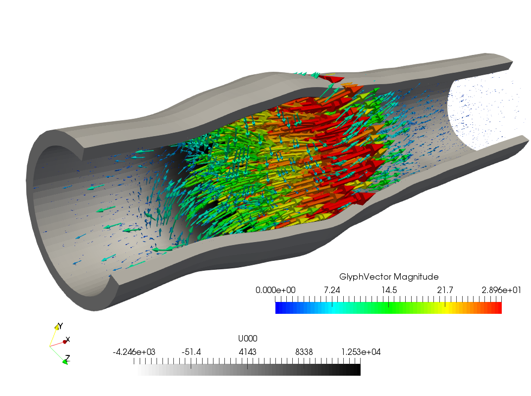
Figure 2: Velocity field of the pressure wave at $t=$0.006\text{\,}\mathrm{s}$$ on the deformed domain (amplified by a factor 10)

If only a do-nothing condition is described with constant pressure at the outflow boundary, then pressure waves are going to be reflected at the outflow boundary. If the pressure along the outflow boundary is chosen appropriate the pressure wave will leave the cylindrical domain without any reflection such that the system will be at rest after some time. To determine the corresponding pressure profile $q(t)\in L^{2}(I)$ on the time interval $I=[0,0.04]$, we minimize the kinetic energy in the fluid domain for $t>$0.03\text{\,}\mathrm{s}$$. Hence we minimize the functional

$$\min_{q\in L^{2}(I)}J(q,\mathbf{v})=\frac{1}{2}\int_{0.03}^{0.04}\lVert\mathbf{v}\rVert^{2}_{\mathcal{F}}\text{ d}t+\frac{\alpha}{2}\int_{0}^{0.04}q(t)^{2}\text{ d}t$$ (31)

constrained by the fluid-structure interaction problem. In time we use, as already in the previous example, a shifted Crank-Nicolson time stepping scheme with time step size $k=0.0001$ and $\theta=0.5+2k$. Only at the time points $t=0$ and $t=0.003$, we use for four steps a time step-size of $k=0.00005$ with $\theta=1.0$. Thereby, no artificial effects occur due to the jump in the pressure at the inflow boundary. The Tikhonov regularization parameter is set to $\alpha=1.0\cdot 10^{-8}$.

mesh level	2	3	4	5	6
spatial dofs 2d	5 540	21 320	83 600	331 040	1 317 440
time steps	$N=600$ uniform time steps (Crank-Nicolson)
spatial dofs 3d	43 904	336 224	894 656	3 122 560	-
time steps	$N=400$ uniform time steps (Crank-Nicolson) plus 8 (back. Euler)

Table 1: Spatial degrees of freedom for 2d and 3d configuration on every refinement level. In 3d the mesh on level 4 and 5 are locally refined along the interface. In time we use a uniform partitioning. In 3d, we add 4 initial backward Euler steps with reduced step size for smoothing at times $t=0\,\mathrm{s}$ and $t=0.03\,\mathrm{s}$ each.

5.3 Optimization algorithm

Given the computed gradient information using Formula (8), we apply a BFGS algorithm implemented in the optimization library RoDoBo [6] to solve the optimization problem. We use a limited memory version as presented e.g. in [22] such that there is no need to assemble and store the BFGS update matrix. To guarantee that the update matrix keeps symmetric and positive definite a Powell-Wolfe step size control should be used. As this step size criteria is in most cases very conservative, we only check if we have descend in the functional value. Control constraints could be added in the optimization algorithm via projection of the update in every optimization step. In this paper we only regard unconstrained examples. Fast convergence of the BFGS algorithm only can be expected close to the optimal solution. Hence, we take advantage of the mesh hierarchy, which is used in the geometric multigrid algorithm, and first solve the optimization problem on a coarse grid to have a good initial guess on finer meshes. As the computation time rises for 3d examples on finer meshes very fast, we can save a lot of computation time using this approach. In the following we reduce the norm of the gradient by a factor of $10^{-1}$ in every optimization loop and then refine the mesh and restart the optimization with the control from the coarser mesh. To compute the gradient, we have to solve the state and dual problem for all time steps. The state solutions are stored on the hard disc and loaded during the computation of the dual problem if necessary. Thereby, only the current state and adjoint solutions have to be held in the memory.

In every Newton step a GMRES iterative solver preconditioned with a geometric multigrid solver provided by the FEM software library Gascoigne [5] is used. All linear systems are solved up to a relative accuracy of $10^{-4}$. In every time step the initial Newton residuum is reduced by a factor of $10^{-6}$. We use the same tolerances for the state and dual problem. The matrices are only reassembled, if the nonlinear convergence rate falls below $\gamma=0.05$ as in [19]. In every dual step, the matrices are assembled at least once at the beginning of every Richardson iteration.

5.4 Numerical results 2d example

In Figure 3 we plot the value of the regularized functional $j(q)$ and the norm of the gradient $\lVert j^{\prime}(q)\rVert$ in every optimization step. The optimization algorithm is started with $q_{n}=0$ for $n=1,\cdots,N$. The computed optimal control is given in Figure 4. The functional value reduces in every optimization step and the gradient can be reduced by a factor of $10^{-3}$ after less then 40 optimization cycles (see Figure 3). In addition we plotted the optimal solution for the 2d example on the finest mesh at the point B in the center of the observation domain $\Omega_{obs}$ and compare the solution to the reference solution in Figure 4. Only around the kink of the desired state a mismatch between desired state and optimized solution can be seen.

Functional $j(q)$	Gradient $\|j^{\prime}(q)\|$

Figure 3: 2d example: Functional value plotted over optimization steps (left), Norm of the gradient plotted over optimization steps (right)

Optimal control $q_{opt}(t)$	Optimal solution $\mathbf{u}_{y}(B)$

Figure 4: 2d example: Optimal control $q_{opt}$ plotted over time (left) and optimal solution and reference solution in the point B plotted over time (right)

To evaluate our approach to solve the optimization algorithm first on coarser grids and then to refine systematically, we restarted the optimization algorithm directly on meshlevel 5. A similar behavior in functional and gradient to the previous approach can be observed in Figure 3. To reduce the gradient to a tolerance of $10^{-12}$ only 20 optimization loops are required. But since about $14\,000\text{\,}\mathrm{s}$ of computational time are needed to solve one cycle of the state and the adjoint system for all time steps on meshlevel 5, but only less then $4000\text{\,}\mathrm{s}$ on the coarser meshlevel 4 (even less time on still coarser grids), systematical refinement of the mesh is much more efficient. The computations were performed on a Intel(R) Xeon(R) Gold 6150 CPU @ 2.70GHz with 18 threads. We parallelized the assembling of matrix and the Vanka smoother as well as the matrix vector multiplication via OpenMP, see [19].

5.5 Numerical Results 3d example

For the 3d example we used the same optimization algorithm as in the 2d case. We can see in Figure 5 that using the optimized pressure profile at the outflow boundary about $98.9\%$ of the kinetic energy after $t>0.03s$ now leaves the cylinder. The jumps in the gradient after every refinement step indicate that a more accurate computation on the coarse grid would not result in better starting values on the finer meshes. The norm of the gradient could be reduced from $1.15\cdot 10^{-4}$ to $3.68\cdot 10^{-7}$ in 23 optimization steps, whereby only 9 optimization cycles were necessary on the computationally costly fine grid on meshlevel 4.

Functional $j(q)$	Gradient $\|j^{\prime}(q)\|$

Figure 5: 3d example: Functional value plotted over optimization steps (left), Norm of the gradient plotted over optimization steps (right)

To compare the controlled solution with the uncontrolled solution, we computed in addition the solution on a cylinder with length $10\text{\,}\mathrm{cm}$. As the reflection on the outflow boundary occurs later the pressure and flow values in the center at $x=$5\text{\,}\mathrm{cm}$$ can be seen as reference values for optimal non reflective boundary conditions for $t<$0.02\text{\,}\mathrm{s}$$. As we only control the pressure on the fluid domain, reflections on the solid boundary can still occur. Furthermore we can observe that the pressure is not constant along the virtual outflow boundary at $x=$5\text{\,}\mathrm{cm}$$ for the long cylinder. Thus, we can not expect the reference solution to fully match the optimized solution. Nevertheless, we can see in Figure 6 that pressure and outflow profiles of the controlled solution are very close to the reference values at the outflow boundary. In addition the kinetic energy in the fluid domain has a similar decay behavior. After the time point $t=$0.025\text{\,}\mathrm{s}$$ the kinetic energy in the left half of the long cylinder rises again due to the reflection of the pressure wave at the outflow boundary at $x=$10\text{\,}\mathrm{cm}$$. This explains the different behavior of pressure and outflow after $t=$0.025\text{\,}\mathrm{s}$$.

Kinetic Energy Fluid	Outflow
Pressure

Figure 6: Kinetic energy in the fluid domain $\mathcal{F}$ as well as outflow and mean pressure plotted over time at $\Gamma_{q}$ for $q=0$, $q_{opt}$ and for a long cylinder

5.6 Test of the Newton scheme, of the Richardson iteration and of the iterative linear solver

How to evaluate the performance of the quasi Newton scheme or of the iterative linear solver is not so obvious. Due to the changing control in every optimization cycle and the nonlinear character of the problem, the condition numbers of the matrices occurring in the linear subproblems will vary in every time step and optimization cycle. Hence, we first compute only one optimization step with $q=0$ on various meshlevels to analyze the h-dependence of our solution algorithm. Thereby, we compare the mean number of Newton/Richardson iterations and GMRES steps per time step on every meshlevel. Afterwards, we compute mean values in every optimization loop to analyze how the performance can vary during the optimization procedure.

mesh	Newton-	Matrix-	GMRES (20)	GMRES (21)	GMRES (22)
level	steps	assemblies	(momentum)	(deformation)	(extension)
3	3.75	0.28	7.19	1.26	3.77
4	3.60	0.87	8.34	1.27	3.82
5	3.91	1.07	9.52	1.25	3.77
6	4.33	1.54	10.61	1.31	3.98
mesh	Richardson-	Matrix-	GMRES (26)	GMRES (27)	GMRES (28)
level	steps	assemblies	(extension)	(deformation)	(momentum)
3	3.09	1.20	4.38	1.32	7.88
4	3.50	1.43	4.80	1.28	8.68
5	3.64	1.48	5.86	1.27	9.54
6	3.69	1.52	6.63	1.27	11.17

Table 2: Average number of Newton/Richardson iterations, average number of matrix assemblies per time step and average number of GMRES steps for solving the three subproblems in the first optimization step. Top: 2d example state, (20) is the coupled momentum equation, (21) the coupling between solid velocity and deformation and (22) the fluid deformation extension. Bottom: 2d example dual, where (26) is the adjoint extension equation, (27) the adjoint solid velocity-deformation coupling and (28) the adjoint coupled momentum equation.

In Table 2 and Table 3 we present the mean number of Newton/Richardson iterations and Matrix assemblies per time step for the 2d and 3d examples. In addition we present the mean number of GMRES steps needed per Newton/Richardson iteration to solve the linear subproblems (22), (21) and (20) and (26), (27) and (28). We can observe that the number of Newton/Richardson iterations per time step ranges between 3 and 4 for state and dual problem. The coupled momentum equation remains the most complex problem with the highest number of steps required. Equations (21) and (27) belong to the discretization of the velocity deformation coupling $d_{t}u=v$ within the solid domain. This corresponds to the inversion of the mass matrix which explains the very low iteration counts. The results for the state equation are similar to the values in [19], where we already could observe for different examples that neglecting the ALE derivatives only has minor influences on the behavior of the Newton scheme. In [19] a more detailed analysis of the smoother in the geometric multigrid algorithm can be found.

As the dual equation is linear with respect to the adjoint variable, we would have expected to need only one Richardson iteration per time step. However, since we neglected terms occurring due to the ALE transformation, we loose the optimal convergence and need about 3 Richardson iterations per time step. On the other hand, the matrices occurring in cascade of subproblems in the dual system have the same condition number as the matrices in the state equation. Only by this approximation and splitting, iterative solvers can successfully be applied to solve the linear problems. The number of GMRES steps in the dual subproblems in Table 2 and Table 3 are rather small and close to the values for the state problem. As (28) and (20) are still fully coupled problems of fluid and elastic solid, most of the computational time is spent in solving these two subproblems. The least number of GMRES steps is needed to invert the mass matrix in (21) and (27). In all subproblems the number of GMRES steps only increases slightly under mesh refinement.

In Figure 7 we show the mean number of GMRES steps per Newton step in every timestep and the number of Newton steps per timestep. For the given examples the values only vary slightly over time. Therefore the mean values in Table 2 and Table 3 represent the overall behavior very well.

To understand how the performance of the solution algorithm in the case of the 2d example varies during the optimization loop, we show in Figure 8 the average number of Newton steps per time step and the average number of GMRES steps per Newton step for each optimization step. The computation was started with $q=0$ on meshlevel 5. No further mesh was applied.

The dependency on the time step size of the presented quasi Newton scheme for the state equation was already analyzed in [19]. Therein, we could observe an increasing Newton iteration count for larger time steps, in particular for very large time steps. A similar behavior can be expected for the dual problem. While the presented solution approach can be regarded as highly efficient and appropriate for optimal control of nonstationary fluid-structure interactions, stationary or quasi stationary applications will call for alternative approaches like the geometric multigrid solver presented by Aulisa, Bna and Bornia [2].

In [19] more details regarding the computational time and savings due to parallelization can be found. As we have to evaluate state and adjoint variables, as well as additional terms due to linearization in every dual step, the computational time to assemble the matrix and to compute the Newton residuum is slightly larger for the dual equation then for the state equation.

mesh	Newton-	Matrix-	GMRES (20)	GMRES (21)	GMRES (22)
level	steps	assemblies	(momentum)	(deformation)	(extension)
2	4.21	0.09	6.82	1.46	2.47
3	3.35	0.80	7.04	1.95	2.60
4	3.46	0.52	7.47	1.91	2.57
5	3.70	0.48	7.34	1.83	2.55
mesh	Richardson-	Matrix-	GMRES (26)	GMRES (27)	GMRES (28)
level	steps	assemblies	(extension)	(deformation)	(momentum)
2	2.99	1.00	2.71	1.35	6.74
3	3.00	1.00	3.30	1.59	7.03
4	2.90	1.00	3.32	1.47	7.06
5	2.39	1.00	3.63	1.51	7.01

Table 3: Average number of Newton/Richardson iterations, average number of matrix assemblies per time step and average number of GMRES steps for solving the three subproblems in the first optimization step. Top: 3d example state, (20) is the coupled momentum equation, (21) the coupling between solid velocity and deformation and (22) the fluid deformation extension. Bottom: 3d example dual, where (26) is the adjoint extension equation, (27) the adjoint solid velocity-deformation coupling and (28) the adjoint coupled momentum equation.

Newton step per time step
Mean GMRES steps per linear solve of (20) and (28)

Figure 7: Performance in first optimization loop on mesh level 5 in 2d (Left) and on mesh level 4 in 3d (Right). Mean GMRES steps per linear solve of (20) and (28) plotted over time steps and number of Newton steps plotted over time steps

Figure 8: Performance in every optimization loop on mesh level 5 in 2d. Left: Mean GMRES steps per linear solve of (20) and (28) plotted over optimization steps . Right: Mean Newton steps per time step plotted over optimization steps

6 Summary

We extended the Newton multigrid framework for monolithic fluid-structure interactions in ALE coordinates presented in [19] to the dual system of fluid-structure interaction problems. The solver is based on replacing the adjoint solid deformation by a new variable and on skipping the ALE derivatives within the adjoint Navier-Stokes equations. As we do not modify the residuum, state and dual solution in each time step still converge to the exact discrete solution. The adjoint coupling conditions incorporated in the monolithic formulation are still fulfilled. As we compute correct gradient information, we see fast convergence in our optimization algorithm. The coupled system is better conditioned (as compared to monolithic Jacobians) which allows to use very simple multigrid smoothers that are easy to parallelize. Only this makes gradient based algorithm feasible and efficient for 3d fluid-structure interaction applications, where memory consumption prevents the use of direct solvers.

It would be straightforward to combine the presented algorithm with dual-weighted residual error estimators for mesh and time step refinement. Instead of global refinement of the mesh after every optimization loop the error estimators indicate where to refine the mesh locally. The sensitivity information from the optimization algorithm can be directly used to evaluate the error estimators.

References

- [1] Asner, L., Hadjicharalambous, M., Chabiniok, R., Peresutti, D., Sammut, E., Wong, J., Carr-White, G., Chowienczyk, P., Lee, J., King, A., et al.: Estimation of passive and active properties in the human heart using 3D tagged MRI. Biomech. Model. Mechanobiol. 15(5), 1121–1139 (2016)
- [2] Aulisa, E., Bna, S., Bornia, G.: A monolithic ale newton-krylov solver with multigrid-richardson-schwarz preconditioning for incompressible fluid-structure interaction. Computers & Fluids 174, 213–228 (2018)
- [3] Bazilevs, Y., Takizawa, K., Tezduyar, T.: Computational Fluid-Structure Interaction: Methods and Applications. Wiley (2013)
- [4] Becker, R., Braack, M.: A finite element pressure gradient stabilization for the Stokes equations based on local projections. Calcolo 38(4), 173–199 (2001)
- [5] Becker, R., Braack, M., Meidner, D., Richter, T., Vexler, B.: The finite element toolkit Gascoigne. https://www.uni-kiel.de/gascoigne/
- [6] Becker, R., Meidner, D., Vexler, B.: The optimal control toolkit RoDoBo. http://www.rodobo.org/
- [7] Bertagna, L., D’Elia, M., Perego, M., Veneziani, A.: Data assimilation in cardiovascular fluid-structure interaction problems: an introduction. In: Fluid-structure interaction and biomedical applications, Adv. Math. Fluid Mech., pp. 395–481. Birkhäuser/Springer, Basel (2014)
- [8] Bertoglio, C., Barber, D., Gaddum, N., Valverde, I., Rutten, M., Beerbaum, P., Moireau, P., Hose, R., Gerbeau, J.: Identification of artery wall stiffness: In vitro validation and in vivo results of data assimilation procedure applied to a 3D fluid-structure interaction model. J. Biomech. 47(5), 1027–34 (2014)
- [9] Bertoglio, C., Chapelle, D., Fernández, M.A., Gerbeau, J.F., Moireau, P.: State observers of a vascular fluid-structure interaction model through measurements in the solid. Comput. Methods Appl. Mech. Engrg. 256, 149–168 (2013). 10.1016/j.cma.2012.12.010. URL http://dx.doi.org/10.1016/j.cma.2012.12.010
- [10] Bertoglio, C., Moireau, P., Gerbeau, J.F.: Sequential parameter estimation for fluid–structure problems: application to hemodynamics. Int. J. Numer. Methods Biomed. Eng. 28(4), 434–455 (2012). 10.1002/cnm.1476. URL http://dx.doi.org/10.1002/cnm.1476
- [11] Braack, M.: Optimal control in fluid mechanics by finite elements with symmetric stabilization. SIAM J. Control Optimization 48(2), 672–687 (2009)
- [12] Braack, M., Richter, T.: Stabilized finite elements for 3-d reactive flows. Int. J. Numer. Meth. Fluids 51, 981–999 (2006). 10.1002/fld.1160
- [13] Causin, P., Gereau, J., Nobile, F.: Added-mass effect in the design of partitioned algorithms for fluid-structure problems. Comput. Methods Appl. Mech. Engrg. 194, 4506–4527 (2005)
- [14] Degroote, J., Hojjat, M., Stavropoulou, E., Wüchner, R., Bletzinger, K.U.: Partitioned solution of an unsteady adjoint for strongly coupled fluid-structure interactions and application to parameter identification of a one-dimensional problem. Struct. Multidiscip. Optim. 47(1), 77–94 (2013). 10.1007/s00158-012-0808-2. URL http://dx.doi.org/10.1007/s00158-012-0808-2
- [15] D’Elia, M., Mirabella, L., Passerini, T., Perego, M., Piccinelli, M., Vergara, C., Veneziani, A.: Modeling of Physiological Flows, MS&A - Modeling, Simulation and Applications, vol. 5, chap. Applications of variational data assimilation in computational hemodynamics, pp. 363–394. Springer Milan (2012)
- [16] Donea, J.: An arbitrary lagrangian-eulerian finite element method for transient dynamic fluid-structure interactions. Comput. Methods Appl. Mech. Engrg. 33, 689–723 (1982)
- [17] Failer, L.: Optimal control for time dependent nonlinear fluid-structure interaction. Ph.D. thesis, Technische Universität München (2017)
- [18] Failer, L., Meidner, D., Vexler, B.: Optimal control of a linear unsteady fluid-structure interaction problem. J. Optim. Theory Appl. 170(1), 1–27 (2016). 10.1007/s10957-016-0930-1. URL http://dx.doi.org/10.1007/s10957-016-0930-1
- [19] Failer, L., Richter, T.: A parallel newton multigrid framework for monolithic fluid-structure interactions. Journal of Scientific Computing 82, 28 (2020). doi 10.1007/s10915-019-01113-y
- [20] Failer, L., Wick, T.: Adaptive time-step control for nonlinear fluid-structure interaction. Journal of Computational Physics 366, 448 – 477 (2018)
- [21] Frei, S.: Eulerian finite element methods for interface problems and fluid-structure interactions. Ph.D. thesis, Universität Heidelberg (2016). Doi:10.11588/heidok.00021590
- [22] Geiger, C., Kanzow, C.: Numerische Verfahren zur Lösung unrestringierter Optimierungsaufgaben. Springer-Verlag (2013)
- [23] Gerbeau, J.F., Vidrascu, M.: A quasi-newton algorithm based on a reduced model for fluid-structure interaction problems in blood flows. ESAIM: Mathematical Modelling and Numerical Analysis 37(4), 631–647 (2003)
- [24] Heywood, J., Rannacher, R., Turek, S.: Artificial boundaries and flux and pressure conditions for the incompressible Navier-Stokes equations. Int. J. Numer. Math. Fluids. 22, 325–352 (1992)
- [25] Hron, J., Turek, S.: Proposal for numerical benchmarking of fluid-structure interaction between an elastic object and laminar incompressible flow. In: H.J. Bungartz, M. Schäfer (eds.) Fluid-Structure Interaction: Modeling, Simulation, Optimization, Lecture Notes in Computational Science and Engineering, pp. 371–385. Springer (2006)
- [26] Hron, J., Turek, S., Madlik, M., Razzaq, M., Wobker, H., Acker, J.: Numerical simulation and benchmarking of a monolithic multigrid solver for fluid-structure interaction problems with application to hemodynamics. In: H.J. Bungartz, M. Schäfer (eds.) Fluid-Structure Interaction II: Modeling, Simulation, Optimization, Lecture Notes in Computational Science and Engineering, pp. 197–220. Springer (2010)
- [27] Lamata, P., Pitcher, A., Krittian, S., Nordsletten, D., Bissell, M.M., Cassar, T., Barker, A.J., Markl, M., Neubauer, S., Smith, N.P.: Aortic relative pressure components derived from four-dimensional flow cardiovascular magnetic resonance. Magn. Reson. Med. 72(4), 1162–1169 (2014)
- [28] Lassila, T., Manzoni, A., Quarteroni, A., Rozza, G.: A reduced computational and geometrical framework for inverse problems in hemodynamics. Int. J. Numer. Methods Biomed. Eng. 29(7), 741–776 (2013). 10.1002/cnm.2559. URL http://dx.doi.org/10.1002/cnm.2559
- [29] Martin, V., Clément, F., Decoene, A., Gerbeau, J.F.: Parameter identification for a one-dimensional blood flow model. In: CEMRACS 2004—mathematics and applications to biology and medicine, ESAIM Proc., vol. 14, pp. 174–200. EDP Sci., Les Ulis (2005)
- [30] Meidner, D., Richter, T.: Goal-oriented error estimation for the fractional step theta scheme. Comput. Methods Appl. Math. 14(2), 203–230 (2014). 10.1515/cmam-2014-0002. URL https://doi.org/10.1515/cmam-2014-0002
- [31] Meidner, D., Richter, T.: A posteriori error estimation for the fractional step theta discretization of the incompressible Navier-Stokes equations. Comput. Methods Appl. Mech. Engrg. 288, 45–59 (2015). 10.1016/j.cma.2014.11.031. URL https://doi.org/10.1016/j.cma.2014.11.031
- [32] Moireau, P., Bertoglio, C., Xiao, N., Figueroa, C.A., Taylor, C.A., Chapelle, D., Gerbeau, J.F.: Sequential identification of boundary support parameters in a fluid-structure vascular model using patient image data. Biomech. Model. Mechanobiol. 12(3), 475–496 (2013). 10.1007/s10237-012-0418-3. URL http://dx.doi.org/10.1007/s10237-012-0418-3
- [33] Molnar, M.: Stabilisierte Finite Elemente für Strömungsprobleme auf bewegten Gebieten. Master’s thesis, Universität Heidelberg (2015)
- [34] Pant, S., Fabrèges, B., Gerbeau, J.F., Vignon-Clementel, I.E.: A methodological paradigm for patient-specific multi-scale cfd simulations: from clinical measurements to parameter estimates for individual analysis. Int. J. Numer. Method. Biomed. Eng. 30(12), 1614–1648 (2014). 10.1002/cnm.2692. URL http://dx.doi.org/10.1002/cnm.2692
- [35] Perego, M., Veneziani, A., Vergara, C.: A variational approach for estimating the compliance of the cardiovascular tissue: an inverse fluid-structure interaction problem. SIAM J. Sci. Comput. 33(3), 1181–1211 (2011). 10.1137/100808277. URL http://dx.doi.org/10.1137/100808277
- [36] Pironneau, O.: An energy preserving monolithic eulerian fluid-structure numerical scheme. Chinese Annals of Mathematics 39 (2016). Preprint at arXiv:1607.08083
- [37] Pironneau, O.: An energy stable monolithic Eulerian fluid-structure numerical scheme with compressible materials. In: P.G. Ciarlet 80th birthday volume (2019). https://arxiv.org/abs/1607.08083
- [38] Rannacher, R.: R. rannacher. finite element solution of diffusion problems with irregular data. Num. Math. 43, 309–327 (1984)
- [39] Richter, T.: Fluid-structure Interactions. Models, Analysis and Finite Elements, Lecture Notes in Computational Science and Engineering, vol. 118. Springer (2017)
- [40] Richter, T., Wick, T.: Finite elements for fluid-structure interaction in ALE and Fully Eulerian coordinates. Comput. Methods Appl. Mech. Engrg. 199(41-44), 2633–2642 (2010)
- [41] Richter, T., Wick, T.: Optimal control and parameter estimation for stationary fluid-structure interaction problems. SIAM J. Sci. Comput. 35(5), B1085–B1104 (2013). 10.1137/120893239. URL http://dx.doi.org/10.1137/120893239
- [42] Richter, T., Wick, T.: On time discretizations of fluid-structure interactions. In: T. Carraro, M. Geiger, S. Körkel, R. Rannacher (eds.) Multiple Shooting and Time Domain Decomposition Methods, Contributions in Mathematical and Computational Science, vol. 9, pp. 377–400. Springer (2015)
- [43] Yirgit, S., Schäfer, M., Heck, M.: Grid movement techniques and their influence on laminar fluid-structure interaction rpoblems. J. Fluids and Structures 24(6), 819–832 (2008)