True experimental reconstruction of quantum states and processes via convex optimization

Abstract

We use a constrained convex optimization (CCO) method to experimentally characterize arbitrary quantum states and unknown quantum processes on a two-qubit NMR quantum information processor. Standard protocols for quantum state and quantum process tomography are based on linear inversion, which often result in an unphysical density matrix and hence an invalid process matrix. The CCO method on the other hand, produces physically valid density matrices and process matrices, with significantly improved fidelity as compared to the standard methods. The constrained optimization problem is solved with the help of a semi-definite programming (SDP) protocol. We use the CCO method to estimate the Kraus operators and characterize gates in the presence of errors due to decoherence. We then assume Markovian system dynamics and use a Lindblad master equation in conjunction with the CCO method to completely characterize the noise processes present in the NMR qubits.

I Introduction

Recent decades have seen tremendous advances in research to engineer high fidelity devices based on quantum technologiesLadd et al. (2010). Characterizing quantum states and quantum processes in such devices is essential to evaluating their performance and is typically achieved via quantum state tomography (QST) James et al. (2001); Long et al. (2001) and quantum process tomography (QPT)O${}^{{}^{\prime}}$Brien et al. (2004); Chuang and Nielsen (1997) protocols. QST and QPT are statistical processes which comprise two basic elementsBartkiewicz et al. (2016): (1) a set of measurements and 2) an estimator which maps the outcomes of the measurements to an estimate of the unknown state or process. Since the ensemble size is finite and systematic errors are inevitable, there is always some ambiguity associated with the estimation of an experimentally created state, which often leads to an unphysical density matrix Miranowicz et al. (2014); Wölk et al. (2019). It is hence imperative to design efficient QST and QPT protocols which result in physically valid density matrices.

Several tomography protocols have been proposed for both finite- and infinite-dimensional systems, mainly based on the least-squares linear inversion methodXin et al. (2017); Li et al. (2017); Miranowicz et al. (2015). They have been successfully demonstrated on various physical systems such as nuclear spin ensembles Vind et al. (2014) and photon polarization states Qi et al. (2017). Several estimation strategies for QST have been proposed as alternatives to the standard methods, such as maximum likelihood estimation (MLE) Shang et al. (2017), model averaging approach Ferrie (2014a), gradient approach for self-guided QST Ferrie (2014b) and compressed sensing QST (Yang et al., 2017). Similar protocols have been proposed for QPT, which include ancilla-assisted QPT Altepeter et al. (2003), simplified QPT Branderhorst et al. (2009), selective QPT using quantum 2-design states Perito et al. (2018), self-consistent QPT Merkel et al. (2013), compressed sensing QPT Rodionov et al. (2014), and adaptive measurement-based QPT Pogorelov et al. (2017). The experimental implementations of these QST and QPT protocols include hardware platforms such as NMR Maciel et al. (2015); Singh et al. (2016a); Gaikwad et al. (2018), superconducting qubits Neeley et al. (2008), nitrogen vacancy centers in diamond Howard et al. (2006); Zhang et al. (2014) and linear optics Schmiegelow et al. (2010); Chapman et al. (2016). A simplified QPT method was developed to experimentally simulate dephasing channels on an NMR quantum processor Wu et al. (2013). All these methods have been reviewed with respect to their physical resource requirements and their efficiency Mohseni et al. (2008).

Despite numerous tomography approaches in existence, most of them do not produce a valid density or process matrix after implementation. On the other hand, protocols such as adaptive measurements and self-guided tomography which produce valid states and processes, involve a large number of projective measurements Struchalin et al. (2016) which are experimentally and computationally resource-intensive. In other methods such as the MLE protocol, one needs to a priori know the noise distribution present in the system Schwemmer et al. (2015). In this work, we have experimentally implemented a method for QST and QPT that resolves the issue of the unphysicality of the experimentally reconstructed density matrix and process matrix. The standard linear inversion based tomography problem has been transformed into a constrained convex optimization (CCO) problem Branderhorst et al. (2008); Huang et al. (2019). The CCO method is based on optimizing a least squares objective function, subject to the positivity condition as a nonlinear constraint and the unit trace condition as a linear constraint. The advantages of the CCO method are that it does not require any prior knowledge about the system and does not use extra ancillary qubits. We demonstrated these advantages of the CCO method by using it to characterize unknown two-qubit quantum states and processes on an NMR quantum information processor. A criterion termed ‘state deviation’ was used to assess how well the reconstructed quantum process fits the result of the tomography. We efficiently computed the complete set of valid Kraus operators corresponding to a given quantum process via unitary diagonalization of the experimentally reconstructed positive process matrix. Finally, a Lindbladian approach was used in conjunction with the CCO method to study NMR noise processes inherent in the system.

This paper is organized as follows: In Section II we describe the formulation of the CCO problem in the context of QST, and present experimental results for the characterization of various two-qubit quantum states. In Section III, we apply the CCO method to QPT and describe experiments to characterize several quantum processes of a two-qubit system. In Section III.1 the CCO QPT method is used to characterize the noise channels which are active during decoherence of two NMR qubits. Section III.2 summarizes a comparison of the CCO QPT method with standard QPT and with simplified QPT methods. Section IV contains a few concluding remarks. The complete set of Kraus operators corresponding to a given quantum process, obtained via the CCO method, is given in Appendix A.

II Quantum State Tomography with Constrained Convex Optimization

Quantum state tomography (QST) is a method to completely characterize an unknown quantum state James et al. (2001). On an ensemble quantum computer such as NMR, standard QST is carried out by measuring the expectation values of a fixed set of basis operatorsVandersypen and Chuang (2005), with the $n$-qubit density operator $\rho$ being represented in the tensor product of the Pauli basis:

$$\rho=\sum_{i=0}^{3}\sum_{j=0}^{3}...\sum_{n=0}^{3}c_{ij...n}\sigma_{i}\otimes\sigma_{j}\otimes...\sigma_{n}$$ (1)

where $c_{00...0}=1/2^{n}$, $\sigma_{0}$ denotes the $2\times 2$ identity matrix and $\sigma_{i},i=1,2,3$ are single-qubit Pauli operators. By choosing appropriate experimental settings, one can determine all expectation values $c_{ij...n}$Singh et al. (2016b) and thereby reconstruct the density matrix.

The standard protocols for QST involve solving linear system of equations of the form

$$Ax=b$$ (2)

where matrix $A$ is referred to as a fixed coefficient matrix, the vector $x$ contains elements of the density matrix which needs to be reconstructed and vector $b$ contains actual experimental dataLong et al. (2001). One can solve for $x$ by simply inverting the above equation and a $\rho$ can be reconstructed which is Hermitian and has unit trace, but there is no guarantee that it will be positive, since the positivity constraint for a density matrix to be valid is not explicitly included in the standard QST protocol.

To always obtain a positive semi-definite density matrix, the linear inversion-based standard QST problem can hence be reformulated as a CCO problem using semi-definite programming (SDP) as follows:

$$\min_{x}\quad{\|Ax-b\|}_{2}$$ (3)

$$s.t.\quad\mathrm{Tr}(\rho)=1$$

$$\rho\geq 0$$

The least-squares objective function given in Eq.3 is defined in Reference Long et al. (2001). The SDP problem stated in Eq.3 was formulated using the YALMIPLofberg (2004) MATLAB package which employs SeDuMiSturm (1999) as the SDP solver. For two qubits, the objective function has to be optimized over 16 real variables. After solving the SDP problem, a valid density matrix is obtained from a least squares fit to the experimental data, which reveals the true quantum state.

To demonstrate the efficacy of CCO-based QST, we experimentally prepared and tomographed several two-qubit quantum states. All the experiments were performed at room temperature on an ensemble of ¹³C-enriched chloroform molecules dissolved in acetone-D6 at room temperature on a Bruker Avance III 600 MHz FT-NMR spectrometer equipped with a QXI probe. We encoded two qubits using the nuclear spins ¹H and ¹³C. The $T_{1}$ spin-lattice relaxation time for proton and carbon are found to be 8 sec and 16.5 sec respectively, while the $T_{2}$ spin-spin relaxation time for proton and carbon was measured to be 2.9 sec and 0.3 sec, respectively. Qubit-selective rf pulses of desired phase were used to implement local rotation gates; a $\frac{\pi}{2}$ rf pulse on ¹H was of duration 9.4 $\mu$s at a 18.14 W power level, while a $\frac{\pi}{2}$ rf pulse on ¹³C was of duration 15.608 $\mu$s at a 179.47 W power level. The molecular structure, NMR parameters, state initialization and NMR circuits to achieve various quantum gates can be found in Reference Gaikwad et al. (2018).

Table 1: Eigenvalues for the two-qubit density matrix, obtained from experimentally reconstructed density matrices via standard and CCO QST.

Quantum state	Standard	CCO
$|00\rangle$	-0.0488, -0.0171, 0.0499, 1.0160	0, 0.0225, 0, 0.9775
$|01\rangle$	-0.0429, -0.0222, 0.0364, 1.0287	0, 0.0067, 0, 0.9933
$|10\rangle$	-0.1486, -0.0911, 0.1915, 1.0482	0, 0.0807, 0, 0.9193
$|11\rangle$	-0.1457, -0.0955, 0.1933, 1.0480	0, 0.0808, 0, 0.9192
$\frac{1}{\sqrt{2}}(|00\rangle+|11\rangle)$	-0.0822, -0.0456, 0.0508, 1.0778	0, 0.0105, 0, 0.9895
$\frac{1}{\sqrt{2}}(|01\rangle-|10\rangle)$	-0.0950, -0.0370, 0.0624, 1.0696	0, 0.0142, 0, 0.9858
$\frac{1}{\sqrt{2}}(|00\rangle-|11\rangle)$	-0.1315, -0.0455, 0.1180, 1.0591	0, 0.0592, 0, 0.9408
$\frac{1}{\sqrt{2}}(|01\rangle+|10\rangle)$	-0.1175, -0.0278, 0.0910, 0.0543	0, 0.0397, 0, 0.9603
$\frac{1}{\sqrt{2}}(|01\rangle+|11\rangle)$	-0.0892, -0.0493, 0.1060, 1.0326	0, 0.0255, 0, 0.9745
$\frac{1}{\sqrt{2}}(|00\rangle+|01\rangle)$	-0.0587, -0.0166, 0.0683, 1.0070	0, 0.0375, 0, 0.9625
$\frac{1}{\sqrt{2}}(|10\rangle+|11\rangle)$	-0.1017, -0.0730, 0.1209, 1.0538	0, 0.0381, 0, 0.9619
$\frac{1}{\sqrt{2}}(|00\rangle+|10\rangle)$	-0.0884, -0.0469, 0.1093, 1.0260	0, 0.0303, 0, 0.9697
$\frac{1}{\sqrt{2}}(|01\rangle+i|11\rangle)$	-0.0936, -0.0436, 0.0987, 1.0385	0, 0.0267, 0, 0.9733
$\frac{1}{\sqrt{2}}(|10\rangle+i|11\rangle)$	-0.1122, -0.0962, 0.1549, 1.0536	0, 0.0544, 0, 0.9456
$\frac{1}{\sqrt{2}}(|00\rangle+i|10\rangle)$	-0.0898, -0.0420, 0.1028, 1.0290	0, 0.0304, 0, 0.9696
$\frac{1}{\sqrt{2}}(|00\rangle+i|01\rangle)$	-0.0862, -0.0379, 0.0837, 1.0405	0, 0.0329, 0, 0.9671
$\frac{1}{2}(|00\rangle+|01\rangle+|10\rangle+|11\rangle)$	-0.0823, -0.0293, 0.0974, 1.0142	0, 0.0293, 0, 0.9707
$\frac{1}{2}(|00\rangle+i|01\rangle+|10\rangle+i|11\rangle)$	-0.0917, -0.0619, 0.1120, 1.0416	0, 0.0298, 0, 0.9702
$\frac{1}{2}(|00\rangle+|01\rangle+i|10\rangle+i|11\rangle)$	-0.0728, -0.0110, 0.0770, 1.0068	0, 0.0298, 0, 0.9702
$\frac{1}{2}(|00\rangle+i|01\rangle+i|10\rangle-|11\rangle)$	-0.0828, -0.0347, 0.0904, 1.0271	0, 0.0234, 0, 0.9766

The fidelity between the theoretically expected ($\rho_{\rm theo}$) and the experimentally reconstructed ($\rho_{\rm expt}$) quantum state were computed using the measureWeinstein et al. (2001):

$${\mathcal{F}}(\rho_{\rm expt},\rho_{\rm theo})=\frac{|{\rm Tr}[\rho_{\rm expt}\rho_{\rm theo}^{\dagger}]|}{\sqrt{{\rm Tr}[\rho_{\rm expt}^{\dagger}\rho_{\rm expt}]{\rm Tr}[\rho_{\rm theo}^{\dagger}\rho_{\rm theo}]}}$$ (4)

The fidelities computed using CCO QST for several different quantum states showed some improvement over those computed using standard QST. However, the main advantage of the CCO QST method is that the experimentally reconstructed density matrix is always positive semi-definite and hence always represents a valid quantum state. The results for various types of states are tabulated in Table 1.

III Quantum Process Tomography with Constrained Convex Optimization

Quantum process tomography (QPT) aims to characterize an unknown quantum process. Any quantum state $\rho$ undergoing a physically valid process can described by a completely positive (CP) map, and an unknown process $\varepsilon$ can be described in the operator-sum representation Kraus et al. (1983):

$$\varepsilon(\rho)=\sum_{i=1}^{d^{2}}E_{i}\rho E_{i}^{\dagger}$$ (5)

where $E_{i}$’s are the Kraus operators satisfying $\sum_{i}E_{i}E_{i}^{\dagger}=I$. The Kraus operators can be expanded using a fixed complete set of basis operators $\{A_{i}\}$ as

$$\varepsilon(\rho)=\sum_{m,n=1}^{d^{2}}\chi_{mn}A_{m}\rho A_{n}^{\dagger}$$ (6)

where $\chi_{mn}=\sum_{i}a_{im}a_{in}^{*}$ is called the process matrix and is a positive Hermitian matrix satisfying the trace preserving constraint $\sum_{m,n}\chi_{mn}A_{n}^{\dagger}A_{m}=\cal{I}$ O${}^{{}^{\prime}}$Brien et al. (2004); Childs et al. (2001). The dimension of the $\chi$ matrix is specified by $n^{4}-n^{2}$ parameters for a Hilbert space of dimension $n$, and hence the computational resources required for its determination scale exponentially with the number of qubits. The $\chi$ matrix can be experimentally determined by preparing a complete set of linearly independent basis operators and and estimating the output state after the map action and finally computing all the elements of $\chi_{mn}$ from these experimentally estimated output states via linear equations of the form:

$$\beta\chi=\lambda$$ (7)

where $\beta$ is a coefficient matrix, vector $\chi$ contains the elements $\{\chi_{mn}\}$ which are to be determined and vector $\lambda$ is the experimental data Childs et al. (2001). Once the $\chi$ matrix is determined, it can be diagonalized by a unitary transformation $U$ and the Kraus operators can be determined from this diagonalized $\chi$ matrix using

$$E_{i}=\sqrt{d_{i}}\sum_{j}U_{ji}A_{j}$$ (8)

where $d_{i}$ are eigenvalues of $\chi$. This reconstruction of the full set of Kraus operators only works if the experimentally determined $\chi$ matrix is positive semidefinite i.e. if the $d_{i}\geq 0$.

The $\chi$ matrix obtained from standard QPT protocols is Hermitian and has unit trace, but there is no assurance that it will be positive. Standard QPT methods could hence lead to an unphysical density matrix which implies that the inversion was not able to optimally fit the experimental data, and more constraints would have to be used to reconstruct the $\chi$ matrix. One viable alternative is the CCO method of reconstruction, which always leads to a valid process matrix. Convex optimization leads to a global optimization of the model parameters which best fit the a priori information. This circumvents the problem of unphysicality in standard QPT methods and the genuine action of noise channels on different input states can be correctly estimated. In case of completely positive trace preserving (CPTP) maps the mathematical formulation of the CCO method for QPT is given by:

$$\min_{\chi}\quad{\|\beta\chi-\lambda\|}_{2}$$ (9)

$$s.t.\quad\sum_{m,n}\chi_{mn}A_{n}^{\dagger}A_{m}=\cal{I}$$

$$\chi\geq 0$$

The CCO problem given in Eq. 9 can be solved efficiently using SDP Lofberg (2004); Sturm (1999). For two qubits we used 16 linearly independent density operators corresponding to quantum states (this choice is not unique): $\{|00\rangle$, $|01\rangle$, $|0+\rangle$, $|0-\rangle$, $|10\rangle$, $|11\rangle$, $|1+\rangle$, $|1-\rangle$, $|+0\rangle$, $|+1\rangle$, $|++\rangle$, $|+-\rangle$, $|-0\rangle$, $|-1\rangle$, $|-+\rangle$ $|--\rangle\}$ where $|+\rangle=(|0\rangle+|1\rangle)/\sqrt{2}$ and $|-\rangle=(|0\rangle+i|1\rangle)/\sqrt{2}$. The dimension of the $\chi$ matrix is $16\times 16$, the number of real independent parameters is 255, and the vector $\chi$ is of dimensions $256\times 1$ (excluding the trace condition). We have to hence optimize the objective function over $256$ real variables. After solving the SDP problem, we obtain a valid $\chi$ matrix, which can be fitted to the experimental data to reveal the true quantum process.

Table 2: Eigenvalues obtained from experimental $\chi$ matrices constructed via standard and CCO QPT.

Quantum operation	Standard QPT	CCO QPT
CNOT	1.0117, 0.1331, -0.1421, 0.1247, 0.0934, 0.0860, 0.0716, 0.0541, 0.0668, -0.1135, -0.0935, -0.0838, -0.0315, -0.0672, -0.0598, -0.0503	0.0077, 0.0201, 0.0245, 0.0438, 0.9038, 0,0,0 0,0,0,0,0,0,0,0
C-$R^{\pi}_{x}$	0.9972, 0.1435, -0.1305, 0.1198, 0.1061, 0.0971, 0.0837, 0.0746, 0.0553, -0.0119, -0.1044, -0.0838, -0.0415, -0.0767, -0.0578, -0.0639	0.0077, 0.0166, 0.0315, 0.0397, 0.9045, 0,0,0, 0,0,0,0,0,0,0,0
Identity	1.0087, 0.1205, -0.0547, 0.0581, 0.0355, -0.0441, -0.0122, -0.0385, -0.0338, -0.0271, -0.0213, -0.0151, 0.0019, 0.0006, -0.0067, 0.0281	0.0166, 0.0357, 0.9477, 0,0,0,0, 0,0,0,0,0,0,0, 0,0

The eigenvalues of experimentally constructed $\chi$ matrices computed via standard and CCO QPT for the control-$R^{\pi}_{x}$, Identity and CNOT operators are depicted in Table 2. As seen from Table 2, the experimentally estimated $\chi$ matrix via standard QPT has some negative eigenvalues which make it unphysical and it does not correspond to a valid quantum operation. On the other hand, all the eigenvalues of experimentally estimated $\chi$ matrix via CCO QPT are positive, which makes it physical and depicts a valid quantum map.

The fidelity of experimentally constructed $\chi_{\rm{expt}}$ matrix with reference to theoretically expected $\chi_{\rm{theo}}$ matrix was calculated using the measureGaikwad et al. (2018):

$${\mathcal{F}}(\chi_{\rm expt},\chi_{\rm theo})=\frac{|{\rm Tr}[\chi_{\rm expt}\chi_{\rm theo}^{\dagger}]|}{\sqrt{{\rm Tr}[\chi_{\rm expt}^{\dagger}\chi_{\rm expt}]{\rm Tr}[\chi_{\rm theo}^{\dagger}\chi_{\rm theo}]}}$$ (10)

The fidelities calculated via standard and CCO methods are given in Table 3: In all three cases, the fidelity $\mathcal{F}$ obtained via CCO method is greater than 0.98, which shows the efficacy of CCO QPT.

Table 3: Two-qubit gate fidelities obtained via standard QPT and CCO QPT.

Quantum process	Standard QPT	CCO QPT
Identity	0.9809	0.9959
CNOT	0.9313	0.9817
control-$R^{\pi}_{x}$	0.9269	0.9831

State fidelity cannot be used as a measure of determining how well the reconstructed process matrix fits the experimental data, as the first element of the density matrix dominates the trace. We hence used another metric termed “Average state deviation” $\Delta_{{\rm avg}}$ to characterize the quantum process Huang et al. (2019):

$$\Delta=\sum_{ij}\frac{(\rm{abs}(\overline{\rho}_{ij}-{\rho_{ij}}))^{2}}{d^{2}}$$ (11)

where $\rm{abs}(z)$ denotes the absolute value of complex number $z$ and $\{\overline{\rho}_{ij}\}$ are elements of the predicted density matrix using experimentally constructed $\chi$ matrix while $\{\rho_{ij}\}$ are elements of ideal gate output. $\Delta_{{\rm avg}}$ is then computed by averaging over all the input states. The smaller the value of $\Delta_{{\rm avg}}$, the better the process matrix fits the raw data, and the better is the performance of the QPT method. The average state deviation $\Delta_{{\rm avg}}$ is given in Table 4, and it can be seen that the performance of CCO QPT is much better than standard QPT as $\Delta_{{\rm avg}}^{{\rm cco}}<<\Delta_{{\rm avg}}^{{\rm std}}$ for all three quantum gates.

Table 4: Average state deviation computed from standard ($\Delta_{{\rm avg}}^{{\rm std}}$) and from CCO ($\Delta_{{\rm avg}}^{{\rm cco}}$) methods.

Quantum process	$\Delta_{{\rm avg}}^{{\rm std}}$	$\Delta_{{\rm avg}}^{{\rm cco}}$
Identity	0.0020	4.3414e-04
CNOT	0.0097	0.0021
control-$R^{\pi}_{x}$	0.0101	0.0018

The QPT protocol can be used to estimate the Kraus operators from the experimental data, which aid in characterizing the corresponding quantum gates in presence of various systematic errors Howard et al. (2006). Three types of errors can occur in the experimentally constructed density/process matrices: (1) statistical errors, (2) systematic errors, and (3) errors due to noisy processes. To investigate the primary source of errors for our experimentally constructed density or process matrices, we numerically simulated the CNOT and control-$R^{\pi}_{x}$ gates in presence of various noisy channels Kofman and Korotkov (2009); Childs et al. (2001). The complete set of Kraus operators for all three gates are given in Appendix A. It turns out that the magnitude of extra elements that we get in the numerically simulated process matrix is of the order of $10^{-4}$ to $10^{-3}$, while the magnitude of extra elements of experimentally reconstructed process matrix using CCO QPT is the order of $10^{-2}$. This clearly indicates that the primary source of error in gate implementation is not decoherence but rather various systematic errors and imperfect state preparation due to pulse miscalibration or rf inhomogeneity Childs et al. (2001).

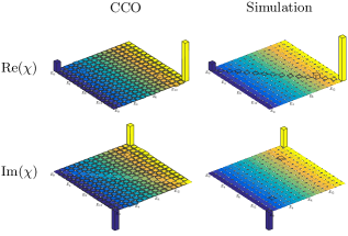
Figure 1: Tomographs denoting the real (top panel) and imaginary (bottom panel) parts of the $\chi$ matrix for system evolving under decoherence for a time $t=0.05$ s. The tomographs in the first and second columns represent the experimentally reconstructed $\chi$ matrix obtained via CCO QPT and via numerical simulation of the decoherence model.

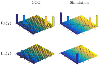
Figure 2: Tomographs denoting the real (top panel) and imaginary (bottom panel) parts of the $\chi$ matrix for system evolving under decoherence for a time $t=0.5$ s. The tomographs in the first and second columns represent the experimentally reconstructed $\chi$ matrix obtained via CCO QPT and via numerical simulation of the decoherence model.

III.1 Markovian Quantum Process Tomography

Standard QPT focuses on making predictions about the output states given an arbitrary set of initial states. However, the standard method is not able to describe the full system dynamics. In the regime of Markovian dynamics, one can construct a valid master equation (called the Lindblad master equation) which describes time evolution of the system, via “snapshots” of the system captured at different time points. In such a scenario, the master equation contains separate terms to describe unitary and non-unitary evolution Howard et al. (2006):

$$\frac{d\rho}{dt}=-i[H,\rho]+\frac{1}{2}\sum_{k=1}^{d^{2}-1}([L_{k}\rho,L_{k}^{\dagger}]+[L_{k},\rho L_{k}^{\dagger}])$$ (12)

where $L_{k}$ are Lindblad operators describing noise processes.

Figure 3: Tomographs denoting the real (top panel) and imaginary (bottom panel) parts of the $\chi$ matrix for system evolving under decoherence for a time $t=5$ s. The tomographs in the first and second columns represent the experimentally reconstructed $\chi$ matrix obtained via CCO QPT and via numerical simulation of the decoherence model.

We now proceed to use CCO QPT to characterize the noise channels acting on the two-qubit NMR system. The relevant time scales are $1/(2J)\approx 2.33$ msec, $\overline{T}_{1}\approx 15$ sec and $\overline{T}_{2}\approx 0.5$ sec where $J$ is scalar spin-spin coupling constant, and $\overline{T}_{1}$ and $\overline{T}_{2}$ are in the range of the longitudinal ($T_{1}$) and transverse ($T_{2}$) relaxation times. We chose four different time intervals: $t_{1}=0.05$ s, $t_{2}=0.5$ s, $t_{3}=5$ s and $t_{4}=15$ s, and computed the $\chi$ matrix for these time points. The real and imaginary parts of the tomographed $\chi$ matrix at the time intervals $t=0.05,0.5,5$ s are shown in Figs. 1- 3, respectively. We compared our experimental results to $\chi_{{\rm num}}$ i.e. the $\chi$ matrix obtained by numerically simulating the decoherence model. The decoherence model took into account the internal Hamiltonian of the system, as well as phase damping and generalized amplitude damping channels acting independently on each qubit. We further studied the evolution of two-qubit maximally entangled Bell states under natural decoherence using QST and then compared the QST results with states predicted using CCO QPT as well as those obtained via numerical simulation of the decoherence model. To investigate the goodness of fit of the decoherence model considered, we calculated process fidelity between experimentally constructed $\chi$ matrix and the numerically simulated $\chi_{num}$ for each time point. For the time intervals $t=0.05$ s, $0.5$ s, $5$ s, and $15$ s, the calculated fidelities are 0.9901, 0.8441, 0.7245 and 0.6724, respectively. This implies that, at small time intervals the process can be modeled well with the decoherence model considered, whereas at longer time intervals the decoherence model needs to be modified by including more termsKofman and Korotkov (2009).

We also studied the behavior of the maximally entangled Bell states: $|{\rm B}_{1}\rangle=(|00\rangle+|11\rangle)/\sqrt{2}$, $|{\rm B}_{2}\rangle=(|01\rangle+|10\rangle)/\sqrt{2}$, $|{\rm B}_{3}\rangle=(|00\rangle-|11\rangle)/\sqrt{2}$ and $|{\rm B}_{4}\rangle=(|01\rangle-|10\rangle)/\sqrt{2}$, under decoherence. We prepared these states with experimental fidelities of 0.9968, 0.9956, 0.9911 and 0.9942, respectively. The fidelity between actual evolved state (constructed via CCO QST) and output state predicted via QPT (both using the experimental and numerical $\chi$ matrix) is given in Table 5. It is evident that for short time intervals (upto $t\approx O(10^{-1})$ s) the decoherence model is able to predict the dynamics of maximally entangled Bell states with fidelities $>0.9$, while CCO QPT is able to predict the true dynamics on all timescales, with good fidelity.

Table 5: The fidelity difference between an actual evolved Bell state (denoted by $|{\rm B}_{i}\rangle$) computed via CCO QPT, and predicted output state QPT. The first column represents the different time intervals for which evolution under the decoherence process was considered.

Process		$|{\rm B}_{1}\rangle$	$|{\rm B}_{2}\rangle$	$~{}~{}~{}|{\rm B}_{3}\rangle$	$~{}~{}~{}|{\rm B}_{4}\rangle~{}~{}~{}$
t=0.05 sec	CCO	0.9672	0.9808	0.9767	0.9902
	Numerical	0.9822	0.9921	0.9844	0.9952
t=0.5 sec	CCO	0.9884	0.9899	0.9891	0.9757
	Numerical	0.9785	0.9795	0.9770	0.9831
t=5 sec	CCO	0.9925	0.8410	0.9946	0.8866
	Numerical	0.6658	0.7193	0.6642	0.7177
t=15 sec	CCO	0.9964	0.9228	0.9959	0.9031
	Numerical	0.6060	0.7121	0.6069	0.7126

III.2 Comparison of CCO QPT with Other Protocols

More often than not, standard QPT protocols lead to unphysical density and processes matrices, which is a major disadvantage. CCO QPT on the other hand, always produces valid density and process matrices, which represent the true quantum state and quantum process. While the experimental complexity is the same for both the methods, the computed state fidelities are better via CCO QPT. The state deviation obtained via CCO QPT is much smaller than that obtained via standard QPT, which indicates its better performance. CCO based QPT allows us to accurately predict the operation of a quantum gate on any arbitrary input state. The experimentally reconstructed $\chi$ matrix via CCO QPT allows us to efficiently compute all Kraus operators, while standard QPT does not even yield valid Kraus operators.

The simplified QPT protocol Wu et al. (2013) requires prior knowledge about the form of the system-environment interaction which is in general not possible. However, CCO QPT does not require any kind of prior knowledge about the system-environment interaction. Simplified QPT is not universal while CCO QPT is universal and is applicable to any physical system of arbitrary dimensions. Both methods produce a valid quantum map and are able to construct all Kraus operators.

IV Conclusions

In this study, we have used a constrained convex optimization (CCO) method to completely characterize various quantum states and quantum processes of two qubits on an NMR quantum information processor. Convex optimization is a search procedure over all operators that satisfies experimental and mathematical constraints in such a way that the solutions that emerge are globally optimal. The results for QST and QPT tomography using CCO, have been compared with those obtained using the standard linear inversion-based methods. Our experiments demonstrate that the CCO method produces physically valid density and process matrices, which closely resemble the quantum state being reconstructed or the quantum process whose evolution is being mapped, respectively. Furthermore, the fidelities obtained via the CCO method are higher as compared to the standard method. We have used the experimentally constructed process matrix to also compute a complete set of Kraus operators corresponding to a given quantum process.

If quantum states are prepared with high fidelity, any discrepancies between the experimental data and reconstructed process matrix cannot be attributed to noise. In such situations, CCO QPT turns out to be a robust method to investigate the nature of the noise processes present in the quantum system. We have assumed system Markovian dynamics and used the CCO method to characterize the decoherence processes inherent to the NMR system. Ongoing efforts in our group include using the CCO method to characterize decoherence present in the system and hence design targeted state preservation protocols. Our results are a step forward in the direction of estimating noise and improving the fidelity of quantum devices.

Appendix A Kraus operators

The complete set of valid Kraus operators for the two-qubit system have been experimentally computed using the CCO QPT method. The Kraus operators corresponding to the Identity, CNOT gate and control-$R^{\pi}_{x}$ gate are given below:

• Kraus operators corresponding to Identity gate

  $$E_{1}={\begin{bmatrix}-0.0308+0.0457i&-0.0028-0.0077i&0.0626+0.1056i&0.0022+0.0078i\\ 0.0070+0.0095i&-0.0393+0.0633i&-0.0055-0.0060i&0.0550+0.1068i\\ 0.0755-0.0678i&0.0203+0.0042i&0.0279-0.0575i&0.0052+0.0001i\\ 0.0395+0.0187i&0.0850+0.0079i&0.0153+0.0005i&0.0451-0.0399i\end{bmatrix}}$$

  $$E_{2}={\begin{bmatrix}0.0571+0.0943i&-0.0133+0.0201i&-0.1932-0.0604i&-0.0069-0.0085i\\ -0.0071+0.0271i&-0.0082+0.0968i&0.0173-0.0019i&-0.1724-0.0574i\\ 0.0189-0.1154i&0.0269-0.0103i&-0.0281-0.1005i&0.0091-0.0038i\\ 0.0481-0.0087i&0.0723-0.0485i&-0.0040+0.0067i&-0.0220-0.0980i\end{bmatrix}}$$

  $$E_{3}={\begin{bmatrix}-0.0442-0.9758i&-0.0014+0.0418i&0.0103+0.0259i&-0.0100-0.0007i\\ 0.0005-0.0271i&-0.0550-0.9813i&0.0095+0.0029i&0.0129+0.0272i\\ 0.0101-0.0239i&0.0088-0.0002i&-0.0190-0.9617i&0.0233+0.0404i\\ -0.0096+0.0017i&0.0101-0.0205i&0.0242-0.0412i&0.0021-0.9671i\\ \end{bmatrix}}$$

• Kraus operators corresponding to CNOT gate

  $$E_{1}={\begin{bmatrix}0.0344-0.0042i&0.0389+0.0130i&-0.0068+0.0035i&-0.0691-0.0003i\\ -0.0039-0.0038i&-0.0208-0.0054i&-0.0494+0.0543i&0.0125+0.0320i\\ 0.0548+0.0194i&-0.0023-0.0251i&-0.0714+0.0137i&-0.0094-0.0117i\\ 0.0208+0.0094i&0.0654+0.0264i&-0.0162+0.0148i&0.0221+0.0124i\end{bmatrix}}$$

  $$E_{2}={\begin{bmatrix}0.0124+0.0245i&0.0065-0.0008i&-0.0508-0.1283i&-0.0079+0.0205i\\ 0.0727+0.0709i&-0.0132-0.0155i&-0.0941+0.0168i&0.0494-0.0326i\\ 0.0323-0.0020i&-0.0552+0.0537i&0.1017+0.0139i&-0.0577-0.0248i\\ 0.0400+0.0811i&-0.0112+0.0281i&0.0603+0.0204i&-0.0381-0.0261i\end{bmatrix}}$$

  $$E_{3}={\begin{bmatrix}0.0907-0.0140i&-0.0599+0.0491i&0.0581+0.0467i&0.0292+0.0058i\\ -0.0567+0.0142i&-0.0978-0.0171i&0.0109+0.0093i&-0.0310-0.1036i\\ 0.0267+0.0135i&-0.0221+0.0546i&-0.0700+0.0595i&-0.0752-0.0404i\\ -0.0269-0.0463i&-0.0340+0.0427i&0.0765+0.0205i&-0.1294+0.0564i\end{bmatrix}}$$

  $$E_{4}={\begin{bmatrix}0.1786+0.0344i&0.1327-0.0629i&0.0228+0.0866i&-0.0018-0.0201i\\ 0.0052-0.0290i&-0.1264-0.0353i&0.0174-0.0797i&-0.0397+0.0932i\\ -0.0346+0.0199i&0.0383-0.0361i&0.1008-0.0337i&-0.1466-0.0222i\\ -0.0024-0.0169i&-0.0415-0.0293i&0.1058-0.0050i&0.1214-0.1034i\end{bmatrix}}$$

  $$E_{5}={\begin{bmatrix}0.0706+0.9517i&-0.0369+0.0847i&0.0250+0.0166i&-0.0245-0.0130i\\ -0.0139-0.1052i&-0.1412+0.9412i&-0.0442-0.0280i&-0.0077-0.0040i\\ -0.0187+0.0169i&-0.0218-0.0073i&-0.0414+0.0215i&-0.0410+0.9380i\\ -0.0065-0.0224i&-0.0537+0.0269i&0.0297+0.9390i&-0.0516+0.0110i\end{bmatrix}}$$

• Kraus operators corresponding to control-$R^{\pi}_{x}$ gate

  $$E_{1}={\begin{bmatrix}0.0012+0.0210i&0.0165+0.0134i&-0.0744+0.0001i&-0.0121-0.0364i\\ 0.0359+0.0089i&0.0251-0.0080i&-0.0654-0.0831i&-0.0097-0.0251i\\ -0.0234+0.0153i&-0.0354-0.0211i&-0.0461+0.0131i&0.0004+0.0068i\\ 0.0365+0.0369i&-0.0233+0.0167i&-0.0068+0.0143i&0.0125-0.0159i\end{bmatrix}}$$

  $$E_{2}={\begin{bmatrix}0.0153+0.0286i&0.0001-0.1142i&-0.0595-0.0245i&0.0153-0.0085i\\ -0.0141+0.0290i&-0.0039-0.0323i&-0.0097+0.0340i&0.1150+0.0166i\\ 0.0058+0.0004i&-0.0092-0.0963i&0.0556+0.0204i&-0.0167-0.0196i\\ -0.0192+0.0136i&-0.0308+0.0298i&0.0407+0.0222i&-0.1054-0.0405i\end{bmatrix}}$$

  $$E_{3}={\begin{bmatrix}0.1537+0.0345i&0.0717+0.0257i&0.0169-0.0805i&-0.0006-0.0094i\\ -0.0074+0.0235i&-0.1425-0.0207i&-0.0232+0.0145i&0.0001-0.0276i\\ 0.0178+0.0428i&-0.0375-0.0168i&0.0243-0.0328i&-0.0154+0.1688i\\ -0.0239-0.0132i&-0.0232+0.0146i&0.0017-0.1398i&0.0512-0.0880i\end{bmatrix}}$$

  $$E_{4}={\begin{bmatrix}0.0686-0.0160i&-0.1101-0.0036i&-0.0419-0.0764i&-0.0257-0.0232i\\ -0.1221-0.0570i&-0.0450+0.0133i&-0.0657+0.0230i&0.0491+0.0496i\\ 0.0651+0.0241i&0.0643-0.0430i&-0.1377+0.1614i&-0.0061+0.0345i\\ -0.0239+0.0021i&-0.0537-0.0392i&-0.0594-0.0210i&0.0213+0.1907i\end{bmatrix}}$$

  $$E_{5}={\begin{bmatrix}0.1841+0.9399i&-0.0704+0.1026i&0.0143+0.0058i&0.0012+0.0004i\\ -0.0949-0.0906i&0.0979+0.9445i&0.0084+0.0134i&-0.0049+0.0210i\\ 0.0077-0.0108i&-0.0075+0.0042i&-0.0249+0.0765i&0.9336-0.0790i\\ -0.0076-0.0216i&-0.0092-0.0086i&0.9304-0.0835i&0.0338+0.0811i\end{bmatrix}}$$