Dynamic Competing Risk Modeling COVID-19
in a Pandemic Scenario

The emergence of coronavirus disease 2019 (COVID-19) in the United States has forced federal and local governments to implement containment measures. Moreover, the severity of the situation has sparked engagement by both the research and clinical community with the goal of developing effective treatments for the disease. This article proposes a time dynamic prediction model with competing risks for the infected individual and develops a simple tool for policy makers to compare different strategies in terms of when to implement the strictest containment measures and how different treatments can increase or suppress infected cases. Two types of containment strategies are compared: (1) a constant containment strategy that could satisfy the needs of citizens for a long period; and (2) an adaptive containment strategy whose strict level changes across time. We consider how an effective treatment of the disease can affect the dynamics in a pandemic scenario. For illustration we consider a region with population 2.8 million and 200 initial infectious cases assuming a 4% mortality rate compared with a 2% mortality rate if a new drug is available. Our results show compared with a constant containment strategy, adaptive containment strategies shorten the outbreak length and reduce maximum daily number of cases. This, along with an effective treatment plan for the disease can minimize death rate.

Keywords: Cumulative incidence function, survival function, adaptive containment measures, pandemic, period of communicability, infectious period

1 Introduction

To prevent the spread of a new infectious disease such as coronavirus disease 2019 (COVID-19), policy makers rely on prediction models to foresee the number of infectious cases and to inform best containment measure strategies including patient quarantine, active monitoring of contacts, border controls, and community education and precautions [20, 17, 10, 13]. There are many prediction models available for this kind of modeling [7, 1, 9, 6, 19, 8, 3, 2, 15, 22]. In predicting local COVID-19 spread, there are two major challenges. Firstly, number of actual infected cases is usually unconfirmed and could be far larger than confirmed cases because there are significant number of infected cases in incubation period and test kits may be insufficient. Secondly, regions that experienced earlier outbreaks can provide valuable information, such as the distribution of cure time, death time, and mortality rate [21], but it is not easy to integrate these dynamic parameters into many current models.

This article provides a simple and robust model framework whose parameters are dynamically adjustable and generally interpretable for policy makers. This framework utilizes competing risks survival analysis to borrow information from regions that experienced earlier outbreaks. Moreover, the model enables containment measures to change over time [5] through introducing a novel transmission number which incorporates containment measures and the basic reproduction number ($R_{0}$).

2 The model

Assume the disease of interest has a $M$-day period of communicability so that infected people are either cured or dead within $M$ days. The value $M$ can also be treated as a parameter in our model. Denote the mortality rate within an infectious period as $m_{\mathrm{death}}$. On day $t$, denote the number of people that have been infected for $d$ days as $p_{t,d}$. The total number of infectious cases at time $t$ is $P_{t}=\sum_{d=1}^{M}p_{t,d}$, where $p_{t,d}$ is determined by the following factors:

1. Mortality rate for people that have been infected for $d$ days, denoted as $m_{d}$.

2. Cure rate for people that have been infected for $d$ days, denoted as $c_{d}$.

3. Average number of people an infectious person can communicate on day $t$, denoted as $R_{t}$.

4. Number of travelers from other areas who have been infected for $d$ days, denoted as $p^{\mathrm{imp}}_{t,d}$.

When moving forward from day $t$ to $t+1$, the number of infectious cases, $P_{t+1}$, is the sum of three terms: (a) the number of survived but uncured cases from day $t$; (b) the number of newly infected cases; and (c) the number of imported cases, denoted as $P^{\text{imp}}_{t+1}=\sum_{d=1}^{M}p^{\mathrm{imp}}_{t,d}$ [4, 14, 18]:

$$P_{t+1}:=\sum_{d=1}^{M}p_{t+1,d}=\sum_{d=1}^{M-1}p_{t,d}(1-m_{d}-c_{d})+P_{t}R_{t}+P_{t+1}^{\mathrm{imp}}.$$ (1)

Here we use $p_{t+1,1}=P_{t}R_{t}$, which counts newly infected cases, and for $d=1,\dots,M-1$, we have $p_{t+1,d+1}=p_{t,d}(1-m_{d}-c_{d})$. Note that the people who have been infected for $M$ days on day $t$ ($p_{t,M}$) will not affect $P_{t+1}$ since their period of communicability will be over and they will be either dead or cured on day $t+1$.

3 Competing risk survival analysis for mortality and cure parameter specification

We use a competing risks framework to specify the mortality rate $m_{d}$ and cure rate $c_{d}$. Let $T$ be the continuous event time of an infected patient. Notice that $T$ is subject to two mutually exclusive competing risks: cure or death. Let $\delta\in\{1,2\}$ be the indicator recording which event occurs; $\delta=1$ denotes cure and $\delta=2$ denotes death.

The cumulative incidence (CIF) is the probability of experiencing an event of type $j$ by time $t$, i.e. $F_{j}(t)=\mathbb{P}\{T\leq t,\delta^{o}=j\}$. The CIF is related to the survival function $S(t)=\mathbb{P}\{T\geq t\}$ by the identity

$$S(t) = 1-\mathbb{P}\{T\leq t\}$$

$$= 1-\left[\mathbb{P}\{T\leq t,\delta=1\}+\mathbb{P}\{T\leq t,\delta=2\}\right]$$

$$= 1-F_{1}(t)-F_{2}(t).$$

The cause-specific hazard $h_{j}$ for event $j$ is given by

$$h_{j}(t)=\lim_{\Delta t\rightarrow 0}\frac{\mathbb{P}\{t\leq T\leq t+\Delta t,\delta=j|T\geq t\}}{\Delta t}=\frac{f_{j}(t)}{S(t)},\qquad\text{}t>0.$$

Thus $h_{j}$ has the following intuitive meaning

$$S(t)h_{j}(t)\asymp\frac{\mathbb{P}\{t\leq T\leq t+\Delta t,\delta=j\}}{\Delta t}.$$

From this, one can deduce that

$$F_{j}(t)=\int_{0}^{t}S(s)h_{j}(s)\,ds=\int_{0}^{t}S(s)\,dH_{j}(s)$$

where $H_{j}(t)=\int_{0}^{t}h_{j}(s)ds$ is the cumulative hazard function (CHF). By the mutual exclusiveness of the two events, the hazard for $T$ is $h(t)=h_{1}(t)+h_{2}(t)$. Because $T$ is a continuous random variable, $S(t)=\exp(-H(t))$ where $H(t)=\int_{0}^{s}h(s)ds$ is the CHF. It follows that

$$F_{j}(t)=\int_{0}^{t}\exp\left(-\int_{0}^{s}\sum_{l=1}^{2}h_{l}(u)du\right)dH_{j}(s)=\int_{0}^{t}\exp(-H_{1}(s))\exp(-H_{2}(s))\,dH_{j}(s).$$ (2)

Let $T_{j}$ be a continuous random variable with hazard $h_{j}$. Keep in mind $T_{j}$ is used only for theoretical construction and is not related to $T$. Let $f_{T_{j}}$ and $F_{T_{j}}$ be the density and cumulative distribution function (CDF) for $T_{j}$. Thus

$$h_{j}(t)=\frac{f_{T_{j}}(t)}{1-F_{T_{j}}(t)}=\frac{f_{T_{j}}(t)}{S_{T_{j}}(t)}$$

where $S_{T_{j}}(t)=\exp(-H_{j}(t))$ is the survival function for $T_{j}$. Using (2), we can rewrite the CIF as

$$F_{j}(t)=\int_{0}^{t}S_{T_{1}}(s)S_{T_{2}}(s)h_{j}(s)\,ds=\int_{0}^{t}S_{T_{1}}(s)S_{T_{2}}(s)\frac{f_{T_{j}}(s)}{S_{T_{j}}(s)}\,ds.$$

Cancelling the common value in numerator and denominator we obtain

$$F_{1}(t)=\int_{0}^{t}S_{T_{2}}(s)\,dF_{1}(s),\qquad\text{}F_{2}(t)=\int_{0}^{t}S_{T_{1}}(s)\,dF_{2}(s).$$ (3)

Identity (3) provides a method for specifying the CIF in terms of the hazard function. A flexible choice is the lognormal hazard. This equals the hazard for the random variable $T_{j}$ that is normally distributed under a log base-e transformation,

$$\ln T_{j}\sim\text{N}(\mu_{j},\sigma_{j}^{2}).$$

Let $\phi_{\mu,\sigma}$ and $\Phi_{\mu,\sigma}$ denote the density and CDF for a $\text{N}(\mu,\sigma^{2})$ random variable. By (3) we have

$$F_{1}(t) = \int_{0}^{t}\mathbb{P}\{T_{2}\geq s\}\,d\mathbb{P}\{T_{1}\leq s\}$$

$$= \int_{0}^{t}\mathbb{P}\{\ln T_{2}\geq\ln s\}\,d\mathbb{P}\{T_{1}\leq s\}$$

$$= \int_{0}^{t}\left[1-\Phi_{\mu_{2},\sigma_{2}}(\ln s)\right]d\mathbb{P}\{T_{1}\leq s\}$$

$$= \int_{0}^{t}d\mathbb{P}\{T_{1}\leq s\}-\int_{0}^{t}\Phi_{\mu_{2},\sigma_{2}}(\ln s)\,d\mathbb{P}\{T_{1}\leq s\}$$

$$= \mathbb{P}\{\ln T_{1}\leq\ln t\}-\int_{0}^{t}\Phi_{\mu_{2},\sigma_{2}}(\ln s)\,d\mathbb{P}\{\ln T_{1}\leq\ln s\}$$

$$= \Phi_{\mu_{1},\sigma_{1}}(\ln t)-\int_{0}^{t}\Phi_{\mu_{2},\sigma_{2}}(\ln s)\,\frac{1}{s}\,\phi_{\mu_{1},\sigma_{1}}(\ln s)\,ds.$$

Similarly, we have

$$F_{2}(t)=\Phi_{\mu_{2},\sigma_{2}}(\ln t)-\int_{0}^{t}\Phi_{\mu_{1},\sigma_{1}}(\ln s)\,\frac{1}{s}\,\phi_{\mu_{2},\sigma_{2}}(\ln s)\,ds.$$

Both $F_{1}$ and $F_{2}$ can be rapidly computed numerically using standard software.

Once the CIF is determined, parameters $m_{d}$ and $c_{d}$ are obtained as follows:

$$m_{d}=\mathbb{P}\{d-1<T\leq d,\delta=2|T\geq d-1\}=\frac{F_{2}(d)-F_{2}(d-1)}{S(d-1)},$$

$$c_{d}=\mathbb{P}\{d-1<T\leq d,\delta=1|T\geq d-1\}=\frac{F_{1}(d)-F_{1}(d-1)}{S(d-1)}.$$ (4)

Note that while the dynamic model (1) implicitly assumes a time window of $[0,M]$, it is not necessary to impose this constraint in the competing risk analysis. This alleviates restrictive assumptions on the survival model, but more importantly allows survival quantities to be fully data driven. This is especially useful when fully nonparametric methods for estimating the CIF are utilized [11].

4 Transmission number specification

The daily transmission numbers $R_{t}$ is determined by the basic reproduction number $R_{0}$, the containment measures on day $t$, and the percentage of uninfected people. It is assumed that cured cases will not get infected again. Since $R_{0}$ is a constant, we only need to set

$$R_{t}=r_{t}\times\frac{P_{\mathrm{pop}}-P_{t}-\sum_{i=1}^{t}(D_{i}+C_{i})}{P_{\mathrm{pop}}},$$

where $D_{i}=\sum_{d=2}^{M}p_{i-1,d}m_{d}$ and $C_{i}=\sum_{d=2}^{M}p_{i-1,d}c_{d}$ are the number of deaths and number of cured patients on day $t=i$ respectively, and $P_{\mathrm{pop}}$ denotes the total population. The crucial parameter is $r_{t}$ which is used to specify the containment scenario. The whole model is comparable to a discrete SIR model [12] where $r_{t}$ serves as the effect contact rate and ${P_{\mathrm{pop}}-P_{t}-\sum_{i=1}^{t}(D_{i}+C_{i})}$ serves as the susceptible population.

For initialization, values are generated from Poisson distribution to mimic the individual variation [16], where $p_{1,d}=\sum_{i=1}^{P_{1}}1\{X_{i}=d\}$, $p^{\text{imp}}_{t,d}=\sum_{j=1}^{P^{\text{imp}}_{t}}1\{X_{j}=d\}$ and $(X_{i},X_{j})_{i,j}$ are independently distributed from a Poisson distribution with mean $\lambda$.

5 Results and conclusion

To compare different pandemic scenarios, consider a region who will experience a COVID-19 outbreak in the scenario illustrated in Table 1. The first set of parameters are disease related and include parameters used for the survival analysis. For this we use a lognormal hazard and we are comparing two treatment plans: for scenario A and B, the mortality rate is $m_{\mathrm{death}}=0.04$ in 50 days, $\sigma_{1}=0.3,\sigma_{2}=0.7$, $\mu_{1}=3.19$ and $\mu_{2}=4.57$; for scenario C, we suppose a new effective drug is available and the mortality rate is $m_{\mathrm{death}}=0.02$ in 40 days, $\sigma_{1}=0.3,\sigma_{2}=0.7$, $\mu_{1}=2.95$ and $\mu_{2}=4.6$. The second set of parameters are population related. The third parameter is $r_{t}$ which defines the containment strategy. For example, $r_{t}=0.21$ from strategy A implies every 100 infected cases will communicate to 21 individuals per day on average. Scenario A adopts a constant containment strategy. Containment strategies for scenarios B and C are the same, which are adaptive and allowed to change weekly. The averages of $r_{t}$ for scenario A, B and C are all 0.21; thus all strategies have the same overall strict level.

Results are displayed in Figure 1. After monitoring 100 simulations, the dynamic of number of infectious cases does not change much from random initialization. In total, numbers of deaths from scenarios A, B and C are $7.20\times 10^{3}$, $5.41\times 10^{3}$ and $2.49\times 10^{3}$; numbers of infected cases are $1.76\times 10^{5}$, $1.32\times 10^{5}$ and $1.28\times 10^{5}$. The number of infectious cases, $P_{t}$, reaches its peak on the 47th, 40th and 40th day and the number of deaths, $D_{t}$, reaches its peak on the 60th, 52th and 49th day for scenarios A, B and C. After the peak of $P_{t}$, the containment strategy does not make much difference on the trend of $P_{t}$ or $D_{t}$.

In conclusion, compared with a constant containment strategy, adaptive containment strategies shorten the outbreak length. Adaptive strategies are less strict at the beginning, which results in more severe spread. However, the stricter measures that are enforced after this have the effect of shortening the outbreak length. Fine tuning these stricter adaptive measures is critical to achieving a minimum death rate and/or reducing maximum daily number of cases. New effective treatment is the key to death rate. Scenario C assumes a new treatment that reduces mortality rate within an infectious period from 4% to 2%, a 50% decrease. When applied in our model, this leads to a decrease in total number of deaths by 53.97%. Importantly, notice this value is larger than 50% as the new treatment reduces the number of infections due to a shorter infectious period and cure time.

Table 1: Necessary inputs for policy makers to compare different scenarios.

Domain	Value	Description
Disease	$M$: $M_{A}=M_{B}=50$	Infected cases will be either cured or dead within $M$ days.
	$\qquad M_{C}=40$	A new effective drug is available in scenario C
	$m_{\mathrm{death}}=4\%\text{ or }2\%$	Within $M$ days, $m_{\mathrm{death}}$ of infected cases will be dead.
	$\sigma_{1}=0.3,\mu_{1}=3.19\text{ or }2.95$	Parameters to shape the cure hazard function.
	$\sigma_{2}=0.7,\mu_{2}=4.57\text{ or }4.6$	Parameters to shape the death hazard function.
People	$P_{\mathrm{pop}}=2.8\times 10^{6}$	On day 1, $P_{\mathrm{pop}}$ people are not infected within the region.
	$P_{1}=200$	On day 1, $P_{1}$ individuals are infectious.
	$P^{\mathrm{imp}}_{15}=P^{\mathrm{imp}}_{48}=2$	On days 15, 29, 48 and 63, there are 2, 4, 2 and 4
	$P^{\mathrm{imp}}_{29}=P^{\mathrm{imp}}_{63}=4$	infectious people who travel into the region.
	$\lambda=16$	Initial infectious cases ($P_{1}$ and $P^{\mathrm{imp}}_{1}$) have been
		infected for $\lambda$ days on average.
Policy	$r_{t}$ described in Figure 1(c)	Smaller value represent stricter containment measures*.

*$r_{t}$ can be interpreted as the average number of newly infected case communicated per infectious person per day on day $t$, if nearly all the population is uninfected. The model will adjust these inputs with percentage of infected cases across time, which produces $R_{t}$.

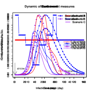
(a)                                       (b)                                     (c)       

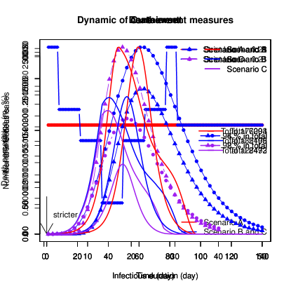
            (d)                                                                (e)       

Figure 1: Comparison of containment strategies and treatment plans for disease using inputs of Table 1. Death and cure rate are plotted in sub-figures (a) and (b), where scenario A and B, colored in blue, have the same mortality rate and a new drug is supposed to be available in scenario C (colored in purple), with lower mortality rate and shorter infectious period. Sub-figure (c) demonstrates the different containment strategies across time. Scenario A (red) has a constant strict level while strictness level is allowed to change weekly for strategies B and C (blue). All containment measures have the same overall strict level. From sub-figures (d) and (e), adaptive containment measures (scenario B and C) result in the smallest number of infected patients and deaths and end the outbreak faster. A new effective drug, illustrated in scenario C, could dramatically decrease the number of deaths and shorten the outbreak length.

Supplement

An online prediction tool is available at  https://minlu.shinyapps.io/killCOVID19/.

References

- [1] C. T. Bauch, J. O. Lloyd-Smith, M. P. Coffee, and A. P. Galvani. Dynamically modeling sars and other newly emerging respiratory illnesses: past, present, and future. Epidemiology, pages 791–801, 2005.
- [2] V. Capasso. Mathematical structures of epidemic systems, volume 97. Springer Science & Business Media, 2008.
- [3] V. Capasso and G. Serio. A generalization of the kermack-mckendrick deterministic epidemic model. Mathematical Biosciences, 42(1-2):43–61, 1978.
- [4] M. Chinazzi, J. T. Davis, M. Ajelli, C. Gioannini, M. Litvinova, S. Merler, A. P. y Piontti, K. Mu, L. Rossi, K. Sun, et al. The effect of travel restrictions on the spread of the 2019 novel coronavirus (covid-19) outbreak. Science, 2020.
- [5] J. Cohen and K. Kupferschmidt. Strategies shift as coronavirus pandemic looms, 2020.
- [6] V. Colizza, A. Barrat, M. Barthelemy, A.-J. Valleron, and A. Vespignani. Modeling the worldwide spread of pandemic influenza: baseline case and containment interventions. PLoS medicine, 4(1), 2007.
- [7] C. Dye and N. Gay. Modeling the sars epidemic. Science, 300(5627):1884–1885, 2003.
- [8] A. Gray, D. Greenhalgh, L. Hu, X. Mao, and J. Pan. A stochastic differential equation sis epidemic model. SIAM Journal on Applied Mathematics, 71(3):876–902, 2011.
- [9] C.-Y. Huang, C.-T. Sun, J.-L. Hsieh, and H. Lin. Simulating sars: Small-world epidemiological modeling and public health policy assessments. Journal of Artificial Societies and Social Simulation, 7(4), 2004.
- [10] D. J. Hunter. Covid-19 and the stiff upper lip—the pandemic response in the united kingdom. New England Journal of Medicine, 2020.
- [11] H. Ishwaran, T. A. Gerds, U. B. Kogalur, R. D. Moore, S. J. Gange, and B. M. Lau. Random survival forests for competing risks. Biostatistics, 15(4):757–773, 2014.
- [12] W. O. Kermack and A. G. McKendrick. A contribution to the mathematical theory of epidemics. Proceedings of the royal society of london. Series A, Containing papers of a mathematical and physical character, 115(772):700–721, 1927.
- [13] K. Kupferschmidt and J. Cohen. Will novel virus go pandemic or be contained?, 2020.
- [14] S. P. Layne, J. M. Hyman, D. M. Morens, and J. K. Taubenberger. New coronavirus outbreak: Framing questions for pandemic prevention, 2020.
- [15] W.-m. Liu, S. A. Levin, and Y. Iwasa. Influence of nonlinear incidence rates upon the behavior of sirs epidemiological models. Journal of mathematical biology, 23(2):187–204, 1986.
- [16] J. O. Lloyd-Smith, S. J. Schreiber, P. E. Kopp, and W. M. Getz. Superspreading and the effect of individual variation on disease emergence. Nature, 438(7066):355–359, 2005.
- [17] Y. Ng, Z. Li, Y. X. Chua, W. L. Chaw, Z. Zhao, B. Er, R. Pung, C. J. Chiew, D. C. Lye, D. Heng, et al. Evaluation of the effectiveness of surveillance and containment measures for the first 100 patients with covid-19 in singapore–january 2–february 29, 2020. 2020.
- [18] G. Pacheco, J. Bustamante-Castañeda, J.-G. Caputo, M. Jiménez-Corona, and S. Ponce-De-León. Dispersion of a new coronavirus sars-cov-2 by airlines in 2020: Temporal estimates of the outbreak in mexico. 2020.
- [19] H. Rahmandad and J. Sterman. Heterogeneity and network structure in the dynamics of diffusion: Comparing agent-based and differential equation models. Management Science, 54(5):998–1014, 2008.
- [20] F. M. Shearer, R. Moss, J. McVernon, J. V. Ross, and J. M. McCaw. Infectious disease pandemic planning and response: Incorporating decision analysis. PLoS Medicine, 17(1), 2020.
- [21] D. L. Wilson. The analysis of survival (mortality) data: fitting gompertz, weibull, and logistic functions. Mechanisms of ageing and development, 74(1-2):15–33, 1994.
- [22] J. Zhang, J. Lou, Z. Ma, and J. Wu. A compartmental model for the analysis of sars transmission patterns and outbreak control measures in china. Applied Mathematics and Computation, 162(2):909–924, 2005.