A Robust Gradient Tracking Method for Distributed Optimization over Directed Networks

Abstract

In this paper, we consider the problem of distributed consensus optimization over multi-agent networks with directed network topology. Assuming each agent has a local cost function that is smooth and strongly convex, the global objective is to minimize the average of all the local cost functions. To solve the problem, we introduce a robust gradient tracking method (R-Push-Pull) adapted from the recently proposed Push-Pull/AB algorithm [1, 2]. R-Push-Pull inherits the advantages of Push-Pull and enjoys linear convergence to the optimal solution with exact communication. Under noisy information exchange, R-Push-Pull is more robust than the existing gradient tracking based algorithms; the solutions obtained by each agent reach a neighborhood of the optimum in expectation exponentially fast under a constant stepsize policy. We provide a numerical example that demonstrate the effectiveness of R-Push-Pull.

I Introduction

We consider a system of $n$ agents communicating through a network to collaboratively solve the following optimization problem:

$$\min\limits_{x\in\mathbb{R}^{p}}~{}f(x):=\frac{1}{n}\sum\limits_{i=1}^{n}f_{i}(x),$$ (1)

where $x$ is the global decision variable and each function $f_{i}:\mathbb{R}^{p}\rightarrow\mathbb{R}$ is known by agent $i$ only. The objective is to obtain an optimal and consensual solution through local updates and local neighbor communications and information exchange. Such local exchange is desirable when sharing a large amount of data is prohibitively expensive due to limited communication resources, or when privacy needs to be preserved for individual agents. Scenarios in which problem (1) is considered include distributed machine learning [3, 4, 5], multi-agent target seeking [6, 7], and wireless networks [8, 9, 10], among many others.

To solve problem (1) in a multi-agent system, many distributed first-order algorithms have been proposed under various assumptions on the objective functions and the underlying network topology [11, 12, 13, 14, 15, 16, 17, 18, 19, 20, 21, 22, 23, 24, 25]. Most works, including [11, 12, 13, 14, 15, 16, 22], often restrict the network connectivity structure to undirected graphs, or more commonly require doubly stochastic mixing matrices. For strongly convex and smooth objective functions, EXTRA [11] first uses a gradient difference structure to achieve the typical linear convergence rates of a centralized gradient method. Recently, the gradient tracking technique has been employed to develop decentralized algorithms which are able to track the average of the gradients [14, 15, 24, 23, 18, 26] and enjoy linear convergence under possibly time-varying graphs.

In this work, we are interested in the scenario where agents interact in a general directed network that includes undirected network as a special case. For directed graphs, constructing a doubly stochastic matrix needs weight balancing which requires an independent iterative process over the network. To avoid such a procedure, most efforts adopted the push-sum technique introduced in [27] for reaching average consensus over directed graphs. The work in [28] first proposed a push-sum based distributed optimization algorithm for directed graphs. In [17], a push-sum based decentralized subgradient method was proposed and analyzed for time-varying directed graphs. For smooth objective functions, the work in [19, 29] modifies the algorithm from [11] with the push-sum technique, thus providing a new algorithm which converges linearly for smooth and strongly convex objective functions.

Equipped with the gradient tracking technique, the algorithms developed in [18, 25, 23, 25, 26] enjoy linear convergence for possibly time-varying directed graphs [23] or under asynchronous updates [26]. Recently, the work in [1, 30, 2] introduced a modified gradient-tracking algorithm called Push-Pull/AB for distributed consensus optimization over directed networks. Unlike the push-sum protocol, Push-Pull uses a row stochastic matrix for the mixing of the decision variables, while it employs a column stochastic matrix for tracking the average gradients. It unifies different computational architectures and can be implemented asynchronously or over time-varying networks [30, 31]. Accelerated version of the algorithm has also been developed [32].

Despite that the aforementioned gradient tracking based algorithms are able to achieve linear convergence over directed networks under the smoothness and strong convexity condition, they are not robust to errors caused by noisy communication links or quantization [33, 34, 35, 36]. Considering noisy information exchange is extremely important in distributed optimization, for example, when one wishes to lower communication bandwidth costs among the agents by performing gradient compression techniques [35, 36], or when there is receiver-side noise corruption of signals in wireless networks [34]. As we will show both theoretically and through experiments, existing gradient tracking based methods fail in this scenario due to inaccurate tracking of the average gradients.

To address the challenge, we propose a novel gradient tracking algorithm (R-Push-Pull) for distributed optimization that is robust to noisy information exchange. R-Push-Pull inherits the advantages of Push-Pull and achieves linear convergence to the optimal solution under noiseless communication links. It also allows for flexible network design and unifies different computational architectures.

Our work is related to the literature in distributed stochastic optimization, where only stochastic gradient information is available (see e.g., [37, 38, 39, 40, 22, 41]) and distributed optimization using quantized information (see e.g., [35, 42, 43]). For instance, the work in [22, 32] combined gradient tracking with stochastic gradient updates and show the iterates convergence linearly to a neighborhood of the optimal solution assuming strongly convex and smooth objectives. The paper [42] studied an exact quantized decentralized gradient descent algorithm which achieves a vanishing mean solution error under customary conditions for quantizers. A recent work [43] considered quantized push-sum for decentralized optimization over directed graphs and establishes subliear convergence to the optimal solution.

I-A Main Contribution

Our main contribution of the paper is summarized as follows. Firstly, we introduce a novel gradient tracking method (R-Push-Pull) for distributed optimization over directed networks. The method achieves linear convergence to the optimal solution for minimizing the sum of smooth and strongly convex objective functions. Secondly, R-Push-Pull addresses the challenge of noisy information exchange. It is shown to be more robust than the other linearly convergent, gradient tracking based algorithms such as Push-Pull/AB, in the sense that the solutions obtained by each agent running R-Push-Pull reach a neighborhood of the optimum in expectation exponentially fast under a constant stepsize policy, while the other competing algorithms lead to divergent solutions. Finally, we provide a numerical example that demonstrate the effectiveness of R-Push-Pull.

I-B Notation

Vectors default to columns if not otherwise specified. Let each agent $i\in\{1,2,\ldots,n\}$ hold a local copy $x_{i}\in\mathbb{R}^{p}$ of the decision variable and an auxiliary variable $s_{i}\in\mathbb{R}^{p}$, where their values at iteration $k$ are denoted by $x_{i,k}$ and $s_{i,k}$, respectively. Denote

$$\mathbf{x}:=[x_{1},x_{2},\ldots,x_{n}]^{\intercal}\in\mathbb{R}^{n\times p},$$

$$\mathbf{s}:=[s_{1},s_{2},\ldots,s_{n}]^{\intercal}\in\mathbb{R}^{n\times p}.$$

Define $F(\mathbf{x})$ to be an aggregate objective function of the local variables, i.e., $F(\mathbf{x}):=\sum_{i=1}^{n}f_{i}(x_{i})$, and let

$$\nabla F(\mathbf{x}):=\left[\nabla f_{1}(x_{1}),\nabla f_{2}(x_{2}),\ldots,\nabla f_{n}(x_{n})\right]^{\intercal}\in\mathbb{R}^{n\times p}.$$

Definition 1

Given an arbitrary vector norm $\|\cdot\|$ on $\mathbb{R}^{n}$, for any $\mathbf{x}\in\mathbb{R}^{n\times p}$, we define

$$\|\mathbf{x}\|:=\left\|\left[\|\mathbf{x}^{(1)}\|,\|\mathbf{x}^{(2)}\|,\ldots,\|\mathbf{x}^{(p)}\|\right]\right\|_{2},$$

where $\mathbf{x}^{(1)},\mathbf{x}^{(2)},\ldots,\mathbf{x}^{(p)}\in\mathbb{R}^{n}$ are columns of $\mathbf{x}$, and $\|\cdot\|_{2}$ represents the usual $2$-norm.

Definition 2

Given a square matrix $\mathbf{M}$, its spectral radius is denoted by $\rho(\mathbf{M})$.

I-C Organization

The rest of this paper is organized as follows. We state the problem of interest in Section II. Then, we introduce the robust Push-Pull algorithm in Section III along with the motivation. We establish the convergence property of R-Push-Pull in Section IV. In Section V we provide a simple numerical example. Section VI concludes the paper.

II Problem Formulation

We consider agents interact with each other in a general directed network (graph). A directed graph is a pair $\mathcal{G}=(\mathcal{V},\mathcal{E})$, where $\mathcal{V}$ is the set of vertices (nodes) and $\mathcal{E}\subseteq\mathcal{V}\times\mathcal{V}$ denotes the edge set consisted of ordered pairs of vertices. Given a nonnegative matrix $\mathbf{M}=[m_{ij}]\in\mathbb{R}^{n\times n}$, the directed graph induced by $\mathbf{M}$ is denoted by $\mathcal{G}_{\mathbf{M}}=(\mathcal{N},\mathcal{E}_{\mathbf{M}})$, where $\mathcal{N}=\{1,2,\ldots,n\}$ and $(j,i)\in\mathcal{E}_{\mathbf{M}}$ if and only if $m_{ij}>0$. For an arbitrary agent $i\in\mathcal{N}$, its in-neighbor set $\mathcal{N}^{\mathrm{in}}_{\mathbf{M},i}$ is defined as the collection of all individual agents that $i$ can actively and reliably pull data from in the graph $\mathcal{G}_{\mathbf{M}}$; we also define its out-neighbor set $\mathcal{N}^{\mathrm{out}}_{\mathbf{M},i}$ as the collection of all individual agents that can passively and reliably receive data from agent $i$.

To solve Problem (1), assume each agent $i$ hold a local copy $x_{i}\in\mathbb{R}^{p}$ of the decision variable. Then Problem (1) can be written in the following equivalent form:

$$\begin{array}[]{c}\min\limits_{x_{1},x_{2}\ldots,x_{n}\in\mathbb{R}^{p}}\sum\limits_{i=1}^{n}f_{i}(x_{i})\\ \text{s.t. }x_{1}=x_{2}=\cdots=x_{n},\end{array}$$ (2)

where the consensus constraint is imposed.

Regarding the objective functions $f_{i}$ in problem (1), we assume the following strong convexity and smoothness conditions.

Assumption 1

Each $f_{i}$ is $\mu$-strongly convex with $L$-Lipschitz continuous gradients, i.e., for any $x,x^{\prime}\in\mathbb{R}^{p}$,

$$\begin{split}&\langle\nabla f_{i}(x)-\nabla f_{i}(x^{\prime}),x-x^{\prime}\rangle\geq\mu\|x-x^{\prime}\|^{2},\\ &\|\nabla f_{i}(x)-\nabla f_{i}(x^{\prime})\|\leq L\|x-x^{\prime}\|.\end{split}$$ (3)

Under Assumption 1, problem (1) has a unique optimal solution $x^{*}\in\mathbb{R}^{1\times p}$.

III A Robust Gradient Tracking Method

We describe the robust Push-Pull Method in Algorithm 1, where $\epsilon_{i,k}\in\mathbb{R}^{p}$ and $\xi_{i,k}\in\mathbb{R}^{p}$ summarize the noise encountered by agent $i$ during the information exchange at step $k$. Sources of the noise include quantization [36] and/or noisy communication links [35].

Algorithm 1: A Robust Push-Pull Method

Choose stepsize $\alpha>0$ and $\gamma,\eta\in(0,1]$,

in-bound mixing/pulling weights $R_{ij}\geq 0$ for all $j\in\mathcal{N}^{\mathrm{in}}_{\mathbf{R},i}$,

and out-bound pushing weights $C_{li}\geq 0$ for all $l\in\mathcal{N}^{\mathrm{out}}_{\mathbf{C},i}$;

Each agent $i$ initializes with any arbitrary $x_{i,0},s_{i,0}\in\mathbb{R}^{p}$;

for $k=0,1,\cdots$, do

for each $i\in\mathcal{N}$,

agent $i$ pushes (noisy) $C_{li}s_{i,k}$ to each $l\in\mathcal{N}^{\mathrm{out}}_{\mathbf{C},i}$;

agent $i$ pulls (noisy) $x_{j,k}$ from each $j\in\mathcal{N}^{\mathrm{in}}_{\mathbf{R},i}$;

for each $i\in\mathcal{N}$,

$\displaystyle\begin{array}[]{ll}&s_{i,k+1}=(1-\gamma)s_{i,k}+\gamma\left(\sum_{j=1}^{n}C_{ij}s_{j,k}+\epsilon_{i,k}\right)\\ &\qquad\qquad+\nabla f_{i}(x_{i,k})\\ &x_{i,k+1}=(1-\eta)x_{i,k}+\eta\left(\sum_{j=1}^{n}R_{ij}x_{j,k}+\xi_{i,k}\right)\\ &\qquad\qquad-\alpha(s_{i,k+1}-s_{i,k})\end{array}$

end for

Denote

$$\boldsymbol{\epsilon}_{k}:=[\epsilon_{1,k},\epsilon_{2,k},\ldots,\epsilon_{n,k}]^{\intercal},\quad\boldsymbol{\xi}_{k}:=[\xi_{1,k},\xi_{2,k},\ldots,\xi_{n,k}]^{\intercal}.$$

We make the following standing assumption.

Assumption 2

Random sequences $\{\boldsymbol{\epsilon}_{k}\}$ and $\{\boldsymbol{\xi}_{k}\}$ are independent. The matrices $\boldsymbol{\epsilon}_{k}$ and $\boldsymbol{\xi}_{k}$ have zero mean and bounded variance, i.e., $\mathbb{E}[\boldsymbol{\epsilon}_{k}]=\mathbb{E}[\boldsymbol{\xi}_{k}]=\mathbf{0}$, $\mathbb{E}[\|\boldsymbol{\epsilon}_{k}\|^{2}]\leq\sigma_{\boldsymbol{\epsilon}}^{2}$, $\mathbb{E}[\|\boldsymbol{\xi}_{k}\|^{2}]\leq\sigma_{\boldsymbol{\xi}}^{2}$ for some $\sigma_{\boldsymbol{\epsilon}},\sigma_{\boldsymbol{\xi}}>0$.

Assumption 2 holds true, for example, when unbiased quantization is performed [36].

Denote

$$\begin{split}&\mathbf{C}:=[C_{ij}],\,\mathbf{C}_{\gamma}:=(1-\gamma)\mathbf{I}+\gamma\mathbf{C},\\ &\mathbf{R}:=[R_{ij}],\,\mathbf{R}_{\eta}:=(1-\eta)\mathbf{I}+\eta\mathbf{R}.\end{split}$$ (4)

We can rewrite Algorithm 1 in the following matrix form:

$$\mathbf{s}_{k+1}=\mathbf{C}_{\gamma}\mathbf{s}_{k}+\gamma\boldsymbol{\epsilon}_{k}+\nabla F(\mathbf{x}_{k}),$$ (5a)

$$\mathbf{x}_{k+1}=\mathbf{R}_{\eta}\mathbf{x}_{k}+\eta\boldsymbol{\xi}_{k}-\alpha(\mathbf{s}_{k+1}-\mathbf{s}_{k}).$$ (5b)

The matrices $\mathbf{R}$ and $\mathbf{C}$ and their induced graphs $\mathcal{G}_{\mathbf{R}}$ and $\mathcal{G}_{\mathbf{C}}$ (respectively) satisfy the same conditions as for Push-Pull [30].

Assumption 3

The matrix $\mathbf{R}\in\mathbb{R}^{n\times n}$ is nonnegative row-stochastic and $\mathbf{C}\in\mathbb{R}^{n\times n}$ is nonnegative column-stochastic, i.e., $\mathbf{R}\mathbf{1}=\mathbf{1}$ and $\mathbf{1}^{\intercal}\mathbf{C}=\mathbf{1}^{\intercal}$. In addition, the diagonal entries of $\mathbf{R}$ and $\mathbf{C}$ are positive. The graphs $\mathcal{G}_{\mathbf{R}}$ and $\mathcal{G}_{\mathbf{C}^{\intercal}}$ each contain at least one spanning tree. Moreover, there exists at least one node that is a root of spanning trees for both $\mathcal{G}_{\mathbf{R}}$ and $\mathcal{G}_{\mathbf{C}^{\intercal}}$.

The readers are referred to Section II of [30] for the motivation of Assumption 3, which differs from most existing works on the assumption of network topology. As a result, R-Push-Pull is flexible in network design and unifies different computational architectures, including (semi-)centralized and decentralized architecture.

Lemma 1

Under Assumption 3, the matrix $\mathbf{R}$ has a nonnegative left eigenvector $u^{\intercal}$ (w.r.t. eigenvalue $1$) with $u^{\intercal}\mathbf{1}=n$, and the matrix $\mathbf{C}$ has a nonnegative right eigenvector $v$ (w.r.t. eigenvalue $1$) with $\mathbf{1}^{\intercal}v=n$ (see [44]).

III-A Algorithm Development

To motivate the development of Algorithm 1, we first take a look at a variant of the Push-Pull algorithm in its matrix form (without noise):

$$\mathbf{x}_{k+1}=\mathbf{R}\mathbf{x}_{k}-\alpha\mathbf{y}_{k},$$ (6a)

$$\mathbf{y}_{k+1}=\mathbf{C}\mathbf{y}_{k}+\nabla F(\mathbf{x}_{k+1})-\nabla F(\mathbf{x}_{k}),$$ (6b)

where $\mathbf{x}_{0}$ is arbitrary and $\mathbf{y}_{0}=\nabla F(\mathbf{x}_{0})$. The matrices $\mathbf{R}$ and $\mathbf{C}$ satisfy Assumption 3. As a result of $\mathbf{C}$ being column-stochastic, we have by induction that

$$\mathbf{1}^{\intercal}\mathbf{y}_{k}=\mathbf{1}^{\intercal}\nabla F(\mathbf{x}_{k}),\qquad\forall k.$$ (7)

Relation (7) is critical for (a subset of) the agents to track the average gradient $\mathbf{1}^{\intercal}\nabla F(\mathbf{x}_{k})/n$ through the $\mathbf{y}$-update. However, this gradient tracking property is not robust. For example, if $y_{i,0}$ are not properly initialized such that $\mathbf{1}^{\intercal}\mathbf{y}_{0}\neq\mathbf{1}^{\intercal}\nabla F(\mathbf{x}_{0})$, then relation (7) will not hold for all $k>0$. Under the scenario of noisy information exchange, instead of relation (7), we have

$$\mathbf{1}^{\intercal}\mathbf{y}_{k}=\mathbf{1}^{\intercal}\nabla F(\mathbf{x}_{k})+\sum_{l=0}^{k-1}\boldsymbol{\xi}_{l},\;\forall k,$$

which suggests that the gradient tracking will incur noise whose variance goes to infinity as $k$ grows.

We remark here that although Push-Pull is not robust to noisy information exchange, it works well with stochastic gradient information under noiseless communication [41, 22]. This is due to the fact that

$$\mathbf{1}^{\intercal}\mathbf{y}_{k}=\mathbf{1}^{\intercal}G(\mathbf{x}_{k}),\;\forall k,$$ (8)

where $G(\mathbf{x}_{k})$ stands for an unbiased estimate of $\nabla F(\mathbf{x}_{k})$. As a result, the (stochastic) gradient tracking is still effective given that $G(\mathbf{x}_{k})$ has bounded variance. We will see below that after a variable transformation, R-Push-Pull resembles Push-Pull while ensuring gradient tracking in the form of (8).

Let $\mathbf{y}_{k}:=\mathbf{s}_{k+1}-\mathbf{s}_{k},\;\forall k$. We have

$$\mathbf{x}_{k+1}=\mathbf{R}_{\eta}\mathbf{x}_{k}+\eta\boldsymbol{\xi}_{k}-\alpha\mathbf{y}_{k},$$ (9a)

$$\mathbf{y}_{k+1}=\mathbf{C}_{\gamma}\mathbf{y}_{k}+\tilde{\nabla}F(\mathbf{x}_{k+1})-\tilde{\nabla}F(\mathbf{x}_{k}),$$ (9b)

where

$$\tilde{\nabla}F(\mathbf{x}_{k}):=\nabla F(\mathbf{x}_{k})+\gamma\boldsymbol{\epsilon}_{k},\;\forall k.$$

This is exactly the Push-Pull update (6) if we ignore the noise and let $\gamma=\eta=1$.

To see why R-Push-Pull is robust in gradient tracking, note that from (5a), we have by induction that

$$\mathbf{1}^{\intercal}\mathbf{s}_{k}=\mathbf{1}^{\intercal}\mathbf{s}_{0}+\sum_{l=0}^{k-1}\mathbf{1}^{\intercal}\tilde{\nabla}F(\mathbf{x}_{k}),\;\forall k.$$

Hence $\mathbf{s}_{k}$ tracks the aggregated gradients of the network over the history. Then from the definition of $\mathbf{y}_{k}$, we have

$$\mathbf{y}_{0}=\mathbf{s}_{1}-\mathbf{s}_{0}=\mathbf{C}_{\gamma}\mathbf{s}_{0}+\tilde{\nabla}F(\mathbf{x}_{0})-\mathbf{s}_{0},$$

indicating that $\mathbf{1}^{\intercal}\mathbf{y}_{0}=\mathbf{1}^{\intercal}\tilde{\nabla}F(\mathbf{x}_{0})$ regardless of the initial choice $\mathbf{s}_{0}$. In addition,

$$\mathbf{1}^{\intercal}\mathbf{y}_{k}=\mathbf{1}^{\intercal}\mathbf{s}_{k+1}-\mathbf{1}^{\intercal}\mathbf{s}_{k}=\mathbf{1}^{\intercal}\tilde{\nabla}F(\mathbf{x}_{k}),\;\forall k,$$ (10)

whose variance is bounded just like in equation (8).

It is worth noting that the robust gradient tracking technique employed by R-Push-Pull, i.e., using $\mathbf{s}_{k}$ and $\mathbf{s}_{k+1}-\mathbf{s}_{k}$ to track the aggregated history gradients and the average gradient at step $k$ respectively, can also be applied to other gradient tracking based methods such as Push-DIGing/ADDOPT [23, 45].

IV Convergence Analysis

In this section, we study the convergence properties of R-Push-Pull. We first define the following variables:

$$\bar{x}_{k}:=\frac{1}{n}u^{\intercal}\mathbf{x}_{k},\ \ \bar{y}_{k}:=\frac{1}{n}\mathbf{1}^{\intercal}\mathbf{y}_{k}.$$

Our strategy is to bound $\mathbb{E}[\|\bar{x}_{k+1}-x^{*}\|_{2}^{2}]$, $\mathbb{E}[\|\mathbf{x}_{k+1}-\mathbf{1}\bar{x}_{k+1}\|_{\mathrm{R}}^{2}]$ and $\mathbb{E}[\|\mathbf{y}_{k+1}-v\bar{y}_{k+1}\|_{\mathrm{C}}^{2}]$ in terms of linear combinations of their previous values, where $\|\cdot\|_{\mathrm{R}}$ and $\|\cdot\|_{\mathrm{C}}$ are specific norms to be defined later. In this way we establish a linear system of inequalities which allows us to derive the convergence results. The proof technique is similar to that of [32, 30] and was inspired by earlier works [24, 25].

IV-A Preliminary Analysis

From relation (9a) and Lemma 1, we have

$$\bar{x}_{k+1}=\frac{1}{n}u^{\intercal}(\mathbf{R}_{\eta}\mathbf{x}_{k}+\eta\boldsymbol{\xi}_{k}-\alpha\mathbf{y}_{k})=\bar{x}_{k}-\frac{\alpha}{n}u^{\intercal}\mathbf{y}_{k}+\frac{\eta}{n}u^{\intercal}\boldsymbol{\xi}_{k}.$$ (11)

By relation (10),

$$\bar{y}_{k}=\frac{1}{n}\mathbf{1}^{\intercal}\tilde{\nabla}F(\mathbf{x}_{k}),\ \ \forall k.$$ (12)

Let us further define

$$h_{k}:=\frac{1}{n}\mathbf{1}^{\intercal}\nabla F(\mathbf{x}_{k})=\frac{1}{n}\sum_{i=1}^{n}f_{i}(x_{i,k}),$$

$$g_{k}:=\frac{1}{n}\mathbf{1}^{\intercal}\nabla F(\mathbf{1}\bar{x}_{k})=\frac{1}{n}\sum_{i=1}^{n}f_{i}(\bar{x}_{k}).$$

Clearly, $\bar{y}_{k}=h_{k}+\frac{\gamma}{n}\mathbf{1}^{\intercal}\boldsymbol{\epsilon}_{k}$. Then, we obtain from relation (11) that

$$\begin{array}[]{l}\bar{x}_{k+1}=\bar{x}_{k}-\frac{\alpha}{n}u^{\intercal}\left(\mathbf{y}_{k}-v\bar{y}_{k}+v\bar{y}_{k}\right)+\frac{\eta}{n}u^{\intercal}\boldsymbol{\xi}_{k}\\ =\bar{x}_{k}-\frac{\alpha}{n}u^{\intercal}v\bar{y}_{k}-\frac{\alpha}{n}u^{\intercal}\left(\mathbf{y}_{k}-v\bar{y}_{k}\right)+\frac{\eta}{n}u^{\intercal}\boldsymbol{\xi}_{k}\\ =\bar{x}_{k}-\tilde{\alpha}g_{k}-\tilde{\alpha}(h_{k}-g_{k})-\frac{\alpha}{n}u^{\intercal}\left(\mathbf{y}_{k}-v\bar{y}_{k}\right)\\ \quad-\tilde{\alpha}\frac{\gamma}{n}\mathbf{1}^{\intercal}\boldsymbol{\epsilon}_{k}+\frac{\eta}{n}u^{\intercal}\boldsymbol{\xi}_{k},\end{array}$$ (13)

where

$$\tilde{\alpha}:=\frac{\alpha}{n}u^{\intercal}v.$$ (14)

In view of (9a) and Lemma 1, using (11) we have

$$\begin{array}[]{ll}\mathbf{x}_{k+1}-\mathbf{1}\bar{x}_{k+1}\\ =\mathbf{R}_{\eta}\mathbf{x}_{k}+\eta\boldsymbol{\xi}_{k}-\alpha\mathbf{y}_{k}-\mathbf{1}\bar{x}_{k}+\alpha\frac{\mathbf{1}u^{\intercal}}{n}\mathbf{y}_{k}-\frac{\mathbf{\eta}u^{\intercal}}{n}\boldsymbol{\xi}_{k}\\ =\mathbf{R}_{\eta}(\mathbf{x}_{k}-\mathbf{1}\bar{x}_{k})-\alpha\left(\mathbf{I}-\frac{\mathbf{1}u^{\intercal}}{n}\right)\mathbf{y}_{k}+\eta(\mathbf{I}-\frac{\mathbf{1}u^{\intercal}}{n})\boldsymbol{\xi}_{k}\\ =\left(\mathbf{R}_{\eta}-\frac{\mathbf{1}u^{\intercal}}{n}\right)(\mathbf{x}_{k}-\mathbf{1}\bar{x}_{k})-\alpha\left(\mathbf{I}-\frac{\mathbf{1}u^{\intercal}}{n}\right)\mathbf{y}_{k}\\ \quad+\eta(\mathbf{I}-\frac{\mathbf{1}u^{\intercal}}{n})\boldsymbol{\xi}_{k},\end{array}$$ (15)

and from (9b) and (12) we obtain

$$\begin{array}[]{ll}\mathbf{y}_{k+1}-v\bar{y}_{k+1}\\ =\mathbf{C}_{\gamma}\mathbf{y}_{k}+\tilde{\nabla}F(\mathbf{x}_{k+1})-\tilde{\nabla}F(\mathbf{x}_{k})-v(\bar{y}_{k+1}-\bar{y}_{k})-v\bar{y}_{k}\\ =\mathbf{C}_{\gamma}\mathbf{y}_{k}-v\bar{y}_{k}+\left(\mathbf{I}-\frac{v\mathbf{1}^{\intercal}}{n}\right)\left(\tilde{\nabla}F(\mathbf{x}_{k+1})-\tilde{\nabla}F(\mathbf{x}_{k})\right)\\ =\left(\mathbf{C}_{\gamma}-\frac{v\mathbf{1}^{\intercal}}{n}\right)(\mathbf{y}_{k}-v\bar{y}_{k})\\ \quad+\left(\mathbf{I}-\frac{v\mathbf{1}^{\intercal}}{n}\right)\left(\tilde{\nabla}F(\mathbf{x}_{k+1})-\tilde{\nabla}F(\mathbf{x}_{k})\right).\end{array}$$ (16)

Denote by $\mathcal{F}_{k}$ the $\sigma$-algebra generated by $\{\boldsymbol{\epsilon}_{0},\boldsymbol{\xi}_{0}\ldots,\boldsymbol{\epsilon}_{k-1},\boldsymbol{\xi}_{k-1}\}$, and define $\mathbb{E}[\cdot\mid\mathcal{F}_{k}]$ as the conditional expectation given $\mathcal{F}_{k}$. We prepare a few useful supporting lemmas for our further analysis, deferred to Appendix VII-A.

IV-B Main Results

The following lemma establishes a linear system of inequalities that bound $\mathbb{E}[\|\bar{x}_{k+1}-x^{*}\|_{2}^{2}]$, $\mathbb{E}[\|\mathbf{x}_{k+1}-\mathbf{1}\bar{x}_{k}\|_{\mathrm{R}}^{2}]$ and $\mathbb{E}[\|\mathbf{y}_{k+1}-v\bar{y}_{k}\|_{\mathrm{C}}^{2}]$.

Lemma 2

Under Assumptions 1-3, when $\tilde{\alpha}\leq 1/(\mu+L)$, we have the following linear system of inequalities:

$$\begin{bmatrix}\mathbb{E}[\|\bar{x}_{k+1}-x^{*}\|_{2}^{2}]\\ \mathbb{E}[\|\mathbf{x}_{k+1}-\mathbf{1}\bar{x}_{k+1}\|_{\mathrm{R}}^{2}]\\ \mathbb{E}[\|\mathbf{y}_{k+1}-v\bar{y}_{k+1}\|_{\mathrm{C}}^{2}]\end{bmatrix}\leq\mathbf{A}\begin{bmatrix}\mathbb{E}[\|\bar{x}_{k}-x^{*}\|_{2}^{2}]\\ \mathbb{E}[\|\mathbf{x}_{k}-\mathbf{1}\bar{x}_{k}\|_{\mathrm{R}}^{2}]\\ \mathbb{E}[\|\mathbf{y}_{k}-v\bar{y}_{k}\|_{\mathrm{C}}^{2}]\end{bmatrix}+\mathbf{B},$$ (17)

where the inequality is to be taken component-wise. The transition matrix $\mathbf{A}=[a_{ij}]$ and the vector $\mathbf{B}$ are given by:

$$\mathbf{A}=\begin{bmatrix}1-\tilde{\alpha}\mu&c_{1}\alpha&c_{2}\alpha\\ c_{5}\alpha^{2}&\frac{1+\tau_{\mathrm{R}}^{2}}{2}+c_{6}\alpha^{2}&c_{7}\alpha^{2}\\ c_{10}\alpha^{2}&c_{11}&\frac{1+\tau_{\mathrm{C}}^{2}}{2}+c_{12}\alpha^{2}\end{bmatrix}$$ (18)

and

$$\mathbf{B}=\begin{bmatrix}c_{3}\alpha^{2}\\ c_{8}\alpha^{2}\\ c_{13}\end{bmatrix}\gamma^{2}\sigma_{\boldsymbol{\epsilon}}^{2}+\begin{bmatrix}c_{4}\\ c_{9}\\ c_{14}\end{bmatrix}\eta^{2}\sigma_{\boldsymbol{\xi}}^{2},$$ (19)

respectively, where constants $c_{1}-c_{13}$ are defined in (35), (38), and (41).

Proof:

See Appendix VII-B. ∎

The following theorem established the convergence properties for R-Push-Pull in (5).

Theorem 1

Suppose Assumptions 1-3 hold and the stepsize $\alpha$ satisfies

$$\alpha\leq\min\left\{\sqrt{\frac{1-\tau_{\mathrm{R}}^{2}}{6c_{6}}},\sqrt{\frac{1-\tau_{\mathrm{C}}^{2}}{6c_{12}}},\sqrt{\frac{2d_{3}}{d_{2}+\sqrt{d_{2}^{2}+4d_{1}d_{3}}}}\right\},$$ (20)

where $d_{1}-d_{3}$ are defined in (27). Then $\sup_{l\geq k}\mathbb{E}[\|\bar{x}_{l}-x^{*}\|_{2}^{2}]$ and $\sup_{l\geq k}\mathbb{E}[\|\mathbf{x}_{l}-\mathbf{1}\bar{x}_{l}\|_{\mathrm{R}}^{2}]$, respectively, converge to $\limsup_{k\rightarrow\infty}\mathbb{E}[\|\bar{x}_{k}-x^{*}\|_{2}^{2}]$ and $\limsup_{k\rightarrow\infty}\mathbb{E}[\|\mathbf{x}_{k}-\mathbf{1}\bar{x}_{k}\|_{\mathrm{R}}^{2}]$ at the linear rate $\mathcal{O}(\rho(\mathbf{A})^{k})$, where $\rho(\mathbf{A})<1$ is the spectral radius of the matrix $\mathbf{A}$. Furthermore,

$$\begin{split}&\limsup_{k\rightarrow\infty}\mathbb{E}[\|\bar{x}_{k}-x^{*}\|_{2}^{2}]\leq[(\mathbf{I}-\mathbf{A})^{-1}\mathbf{B}]_{1},\\ &\limsup_{k\rightarrow\infty}\mathbb{E}[\|\mathbf{x}_{k}-\mathbf{1}\bar{x}_{k}\|_{\mathrm{R}}^{2}]\leq[(\mathbf{I}-\mathbf{A})^{-1}\mathbf{B}]_{2},\end{split}$$ (21)

where $[(\mathbf{I}-\mathbf{A})^{-1}\mathbf{B}]_{j}$ denotes the $j$-th element of the vector $[(\mathbf{I}-\mathbf{A})^{-1}\mathbf{B}]$. Their specific forms are given in (29) and (30) respectively.

Proof:

In light of Lemma 2, by induction we have

$$\begin{bmatrix}\mathbb{E}[\|\bar{x}_{k}-x^{*}\|_{2}^{2}]\\ \mathbb{E}[\|\mathbf{x}_{k}-\mathbf{1}\bar{x}_{k}\|_{\mathrm{R}}^{2}]\\ \mathbb{E}[\|\mathbf{y}_{k}-v\bar{y}_{k}\|_{\mathrm{C}}^{2}]\end{bmatrix}\leq\mathbf{A}^{k}\begin{bmatrix}\mathbb{E}[\|\bar{x}_{0}-x^{*}\|_{2}^{2}]\\ \mathbb{E}[\|\mathbf{x}_{0}-\mathbf{1}\bar{x}_{0}\|_{\mathrm{R}}^{2}]\\ \mathbb{E}[\|\mathbf{y}_{0}-v\bar{y}_{0}\|_{\mathrm{C}}^{2}]\end{bmatrix}+\sum_{l=0}^{k-1}\mathbf{A}^{l}\mathbf{B}.$$ (22)

If the spectral radius of $\mathbf{A}$ satisfies $\rho(\mathbf{A})<1$, then $\mathbf{A}^{k}$ converges to $\mathbf{0}$ at the linear rate $\mathcal{O}(\rho(\mathbf{A})^{k})$ (see [44]), in which case $\sup_{l\geq k}\mathbb{E}[\|\bar{x}_{l}-x^{*}\|^{2}]$, $\sup_{l\geq k}\mathbb{E}[\|\mathbf{x}_{l}-\mathbf{1}\bar{x}_{l}\|^{2}]$ and $\sup_{l\geq k}\mathbb{E}[\|\mathbf{y}_{l}-\mathbf{1}\bar{y}_{l}\|^{2}]$ all converge to a neighborhood of $0$ at the linear rate $\mathcal{O}(\rho(\mathbf{A})^{k})$.

The next lemma provides conditions that ensure $\rho(\mathbf{A})<1$.

Lemma 3

(Lemma 5 in [22]) Given a nonnegative, irreducible matrix $\mathbf{M}=[m_{ij}]\in\mathbb{R}^{3\times 3}$ with $m_{11},m_{22},m_{33}<\lambda^{*}$ for some $\lambda^{*}>0$. A necessary and sufficient condition for $\rho(\mathbf{M})<\lambda^{*}$ is $\text{det}(\lambda^{*}\mathbf{I}-\mathbf{M})>0$.

In light of Lemma 3, it suffices to ensure $a_{11},a_{22},a_{33}<1$ and $\text{det}(\mathbf{I}-\mathbf{A})>0$, or more aggressively,

$$\begin{split}&\text{det}(\mathbf{I}-\mathbf{A})=(1-a_{11})(1-a_{22})(1-a_{33})-a_{12}a_{23}a_{31}\\ &\quad-a_{13}a_{21}a_{32}-(1-a_{22})a_{13}a_{31}-(1-a_{11})a_{23}a_{32}\\ &\quad-(1-a_{33})a_{12}a_{21}>\frac{1}{2}(1-a_{11})(1-a_{22})(1-a_{33}),\end{split}$$ (23)

which is equivalent to

$$\begin{split}&\frac{1}{2}(1-a_{11})(1-a_{22})(1-a_{33})-c_{1}c_{7}c_{10}\alpha^{5}\\ &\quad-c_{2}c_{5}c_{11}\alpha^{3}-(1-a_{22})c_{2}c_{10}\alpha^{3}-(1-a_{11})c_{7}c_{11}\alpha^{2}\\ &\quad-(1-a_{33})c_{1}c_{5}\alpha^{3}>0.\end{split}$$ (24)

We now provide some sufficient conditions under which $a_{11},a_{22},a_{33}<1$ and (24) holds true.

First, $a_{11}<1$ is ensured by choosing $\tilde{\alpha}\leq 1/(\mu+L)$, and $a_{22},a_{33}<1$ is guaranteed by

$$1-a_{22}\geq\frac{1}{3}(1-\tau_{\mathrm{R}}^{2}),\,1-a_{33}\geq\frac{1}{3}(1-\tau_{\mathrm{C}}^{2}),$$ (25)

which requires

$$\alpha\leq\min\left\{\sqrt{\frac{1-\tau_{\mathrm{R}}^{2}}{6c_{6}}},\sqrt{\frac{1-\tau_{\mathrm{C}}^{2}}{6c_{12}}}\right\}.$$ (26)

Second, notice that $a_{22}>\frac{1+\tau_{\mathrm{R}}^{2}}{2}$ and $a_{33}>\frac{1+\tau_{\mathrm{C}}^{2}}{2}$. In light of (25), a sufficient condition for $\text{det}(\mathbf{I}-\mathbf{A})>0$ is to substitute the first $(1-a_{22})$ (respectively, $(1-a_{33})$) in (24) by $(1-\tau_{\mathrm{R}}^{2})/3$ (respectively, $(1-\tau_{\mathrm{C}}^{2})/3$), and substitute the second $(1-a_{22})$ (respectively, $(1-a_{33})$) by $(1-\tau_{\mathrm{R}}^{2})/2$ (respectively, $(1-\tau_{\mathrm{C}}^{2})/2$). We then have

$$d_{1}\alpha^{4}+d_{2}\alpha^{2}-d_{3}<0,$$

where

$$\begin{split}&d_{1}:=c_{1}c_{7}c_{10}\\ &d_{2}:=c_{2}c_{5}c_{11}+\frac{(1-\tau_{\mathrm{R}}^{2})}{2}c_{2}c_{10}+\mu u^{\intercal}vc_{7}c_{11}\\ &\quad+\frac{(1-\tau_{\mathrm{C}}^{2})}{2}c_{1}c_{5}\\ &d_{3}:=\frac{\mu u^{\intercal}v(1-\tau_{\mathrm{R}}^{2})(1-\tau_{\mathrm{C}}^{2})}{18}.\end{split}$$ (27)

Hence

$$\alpha^{2}\leq\frac{2d_{3}}{d_{2}+\sqrt{d_{2}^{2}+4d_{1}d_{3}}}.$$ (28)

Relations (26) and (28) yield the final bound on $\alpha$.

Relation (21) follows from (22) directly given that $\rho(\mathbf{A})<1$. In light of (23) and (25), we obtain from (22) that

$$\begin{split}&[(\mathbf{I}-\mathbf{A})^{-1}\mathbf{B}]_{1}\\ &=\left[((1-a_{22})(1-a_{33})-a_{23}a_{32})(c_{3}\alpha^{2}\gamma^{2}\sigma_{\boldsymbol{\epsilon}}^{2}+c_{4}\eta^{2}\sigma_{\boldsymbol{\xi}}^{2})\right.\\ &\quad+(a_{13}a_{32}+a_{12}(1-a_{33}))(c_{8}\alpha^{2}\gamma^{2}\sigma_{\boldsymbol{\epsilon}}^{2}+c_{9}\eta^{2}\sigma_{\boldsymbol{\xi}}^{2}))\\ &\quad\left.+(a_{12}a_{23}+a_{13}(1-a_{22}))(c_{13}\gamma^{2}\sigma_{\boldsymbol{\epsilon}}^{2}+c_{14}\eta^{2}\sigma_{\boldsymbol{\xi}}^{2}))\right]\frac{1}{\text{det}(\mathbf{I}-\mathbf{A})}\\ &\leq\left[\left(\frac{(1-\tau_{\mathrm{R}}^{2})(1-\tau_{\mathrm{C}}^{2})}{4}-c_{7}c_{11}\alpha^{2}\right)(c_{3}\alpha^{2}\gamma^{2}\sigma_{\boldsymbol{\epsilon}}^{2}+c_{4}\eta^{2}\sigma_{\boldsymbol{\xi}}^{2}))\right.\\ &\quad+\left(c_{2}c_{11}\alpha+\frac{c_{1}(1-\tau_{\mathrm{C}}^{2})\alpha}{2}\right)(c_{8}\alpha^{2}\gamma^{2}\sigma_{\boldsymbol{\epsilon}}^{2}+c_{9}\eta^{2}\sigma_{\boldsymbol{\xi}}^{2}))\\ &\quad\left.+\left(c_{1}c_{7}\alpha^{3}+\frac{c_{2}(1-\tau_{\mathrm{R}}^{2})\alpha}{2}\right)(c_{13}\gamma^{2}\sigma_{\boldsymbol{\epsilon}}^{2}+c_{14}\eta^{2}\sigma_{\boldsymbol{\xi}}^{2}))\right]\\ &\quad\cdot\frac{18}{\tilde{\alpha}\mu(1-\tau_{\mathrm{R}}^{2})(1-\tau_{\mathrm{C}}^{2})},\end{split}$$ (29)

and

$$\begin{split}&[(\mathbf{I}-\mathbf{A})^{-1}\mathbf{B}]_{2}\\ &=\left[(a_{23}a_{31}+a_{21}(1-a_{33}))(c_{3}\alpha^{2}\gamma^{2}\sigma_{\boldsymbol{\epsilon}}^{2}+c_{4}\eta^{2}\sigma_{\boldsymbol{\xi}}^{2})\right.\\ &\quad+((1-a_{11})(1-a_{33})-a_{13}a_{31})(c_{8}\alpha^{2}\gamma^{2}\sigma_{\boldsymbol{\epsilon}}^{2}+c_{9}\eta^{2}\sigma_{\boldsymbol{\xi}}^{2})\\ &\quad\left.+(a_{13}a_{21}+a_{23}(1-a_{11}))(c_{13}\gamma^{2}\sigma_{\boldsymbol{\epsilon}}^{2}+c_{14}\eta^{2}\sigma_{\boldsymbol{\xi}}^{2})\right]\frac{1}{\text{det}(\mathbf{I}-\mathbf{A})}\\ &\leq\left[\left(c_{7}c_{10}\alpha^{4}+c_{5}\alpha^{2}\frac{(1-\tau_{\mathrm{C}}^{2})}{2}\right)(c_{3}\alpha^{2}\gamma^{2}\sigma_{\boldsymbol{\epsilon}}^{2}+c_{4}\eta^{2}\sigma_{\boldsymbol{\xi}}^{2})\right.\\ &\quad+\left(\tilde{\alpha}\mu\frac{(1-\tau_{\mathrm{C}}^{2})}{2}-c_{2}c_{10}\alpha^{3}\right)(c_{8}\alpha^{2}\gamma^{2}\sigma_{\boldsymbol{\epsilon}}^{2}+c_{9}\eta^{2}\sigma_{\boldsymbol{\xi}}^{2})\\ &\quad\left.+\left(c_{2}c_{5}\alpha^{3}+c_{7}\alpha^{2}\tilde{\alpha}\mu\right)(c_{13}\gamma^{2}\sigma_{\boldsymbol{\epsilon}}^{2}+c_{14}\eta^{2}\sigma_{\boldsymbol{\xi}}^{2})\right]\\ &\quad\cdot\frac{18}{\tilde{\alpha}\mu(1-\tau_{\mathrm{R}}^{2})(1-\tau_{\mathrm{C}}^{2})}.\\ \end{split}$$ (30)

∎

From Theorem 1, if $\sigma_{\boldsymbol{\epsilon}}=\sigma_{\boldsymbol{\xi}}=\mathbf{0}$ (no noise), we have $\mathbf{B}=\mathbf{0}$, then R-Push-Pull converges linearly to the optimal solution $x^{*}$. Specifically, when $\alpha$ is sufficiently small, it can be shown that the linear rate indicator $\rho(\mathbf{A})\simeq 1-\tilde{\alpha}\mu$.

The upper bounds in (29) and (30) are functions of $\alpha$, $\eta$, $\gamma$ and other problem parameters, and they are decreasing in the variances $\sigma_{\boldsymbol{\epsilon}}$ and $\sigma_{\boldsymbol{\xi}}$. It can also be numerically verified that $\limsup_{k\rightarrow\infty}\mathbb{E}[\|\bar{x}_{k}-x^{*}\|_{2}^{2}]$ and $\limsup_{k\rightarrow\infty}\mathbb{E}[\|\mathbf{x}_{k}-\mathbf{1}\bar{x}_{k}\|_{\mathrm{R}}^{2}]$ decrease in the stepsize $\alpha$. Moreover, in order to mitigate the effect of noise $\boldsymbol{\epsilon}_{k}$ on the final optimization error, we may take $\eta$ to be in the order of $\mathcal{O}(\alpha)$.

V Numerical Example

We provide a simple illustration example. Consider the Ridge regression problem, i.e.,

$$\min_{x\in\mathbb{R}^{p}}f(x)=\frac{1}{n}\sum_{i=1}^{n}f_{i}(x)\left(=\left(u_{i}^{\intercal}x-v_{i}\right)^{2}+\rho\|x\|^{2}\right),$$ (31)

where $\rho>0$ is a penalty parameter. Each agent $i$ has sample $(u_{i},v_{i})$ with $u_{i}\in\mathbb{R}^{p}$ representing the features and $v_{i}\in\mathbb{R}$ being the observed outputs. Let each $u_{i}\in[-1,1]^{p}$ be generated from uniform distribution, and $v_{i}$ is drawn according to $v_{i}=u_{i}^{\intercal}\tilde{x}_{i}+\varepsilon_{i}$, where parameters $\tilde{x}_{i}$ are evenly located in $[0,10]^{p}$, and $\varepsilon_{i}\sim\mathcal{N}(0,25)$. Given these predetermined parameters, Problem (31) has a unique solution $x^{*}=(\sum_{i=1}^{n}[u_{i}u_{i}^{\intercal}]+n\rho\mathbf{I})^{-1}\sum_{i=1}^{n}[u_{i}u_{i}^{\intercal}]\tilde{x}_{i}$.

We compare the performance of R-Push-Pull against other two gradient tracking based algorithms Push-Pull/AB [1, 2] and Push-DIGing/ADDOPT [23, 45]. To model noisy information exchange, we assume the transmitted values such as $x_{i,k}$, $C_{li}y_{i,k}$ and $C_{li}s_{i,k}$ are corrupted with independent Gaussian noises $\mathcal{N}(0,0.01)$. Regarding the network topology, we generate a directed graph $\mathcal{G}$ of $15$ nodes by adding random links to a ring network, where a directed link exists between any two nonadjacent nodes with probability $0.3$. Then for R-Push-Pull and Push-Pull, we let $\mathcal{G}_{\mathbf{R}}=\mathcal{G}_{\mathbf{C}}=\mathcal{G}$ for simplicity.

Design matrix $\mathbf{C}$ as follows: for any agent $i$, $C_{li}=\frac{1}{|\mathcal{N}^{\mathrm{out}}_{\mathbf{C},i}|+1}$ for all $l\in\mathcal{N}^{\mathrm{out}}_{\mathbf{C},i}$ and $C_{ii}=1-\sum_{l\in\mathcal{N}^{\mathrm{out}}_{\mathbf{C},i}}C_{li}$. Letting $\gamma=0.5$, the same $\mathbf{C}_{\gamma}$ is used for all the algorithms. In R-Push-Pull and Push-Pull, for any agent $i$, $R_{ij}=\frac{1}{|\mathcal{N}^{\mathrm{in}}_{\mathbf{R},i}|+1}$ for all $j\in\mathcal{N}^{\mathrm{in}}_{\mathbf{R},i}$, and $R_{ii}=1-\sum_{j\in\mathcal{N}^{\mathrm{in}}_{\mathbf{R},i}}R_{ij}$. The matrix $\mathbf{R}_{\eta}$ is constructed by taking $\eta=0.01$.

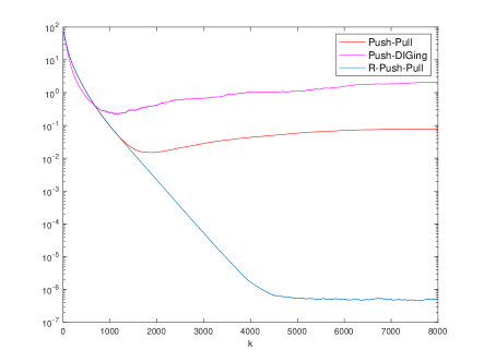
Figure 1: Comparison of the performance of R-Push-Pull, Push-Pull/AB and Push-DIGing/ADDOPT, measured by $\frac{1}{n}\mathbb{E}[\|x_{i,k}-x^{*}\|^{2}]$. The expected errors are approximated by averaging over $50$ simulation results. Dimension $p=10$, stepsize $\alpha=0.01$ and penalty parameter $\rho=0.01$.

Fig. 1 compares the performance of different algorithms with respect to $\frac{1}{n}\mathbb{E}[\|x_{i,k}-x^{*}\|^{2}]$. It can be seen that initially all the errors decrease exponentially fast at comparable rates. However, the errors for Push-Pull/AB and Push-DIGing/ADDOPT eventually increase over time while R-Push-Pull achieves linear convergence to a small neighborhood of $0$. This sharp contrast verifies the effectiveness of the proposed algorithm.

VI Conclusions

In this paper, we introduce a robust gradient tracking method (R-Push-Pull) for distributed optimization over directed networks. R-Push-Pull inherits the advantage of Push-pull and achieves linear convergence to the optimal solution with exact information fusion. Under noisy information exchange, R-Push-Pull is more robust than the other gradient tracking based algorithms. We show the solutions obtained by each agent reach a neighborhood of the optimum in expectation exponentially fast under a constant stepsize policy. We also provide a numerical example that demonstrate the effectiveness of R-Push-Pull.

VII APPENDIX

VII-A Supporting Lemmas

Lemma 4

Under Assumption 1, there holds

$$\|h_{k}-g_{k}\|_{2}\leq\frac{L}{\sqrt{n}}\|\mathbf{x}_{k}-\mathbf{1}\bar{x}_{k}\|_{2},$$ (32a)

$$\mathbb{E}[\|\bar{y}_{k}-h_{k}\|_{2}^{2}\mid\mathcal{F}_{k}]\leq\frac{\gamma^{2}\sigma_{\boldsymbol{\epsilon}}^{2}}{n},$$ (32b)

$$\|g_{k}\|_{2}\leq L\|x_{k}-x^{*}\|_{2}.$$ (32c)

In addition, when $\tilde{\alpha}\leq 2/(\mu+L)$, we have

$$\|\bar{x}_{k}-\tilde{\alpha}g_{k}-x^{*}\|_{2}\leq(1-\tilde{\alpha}\mu)\|\bar{x}_{k}-x^{*}\|_{2},\ \ \forall k.$$ (33)

Proof:

In light of Assumption 1,

$$\|h_{k}-g_{k}\|_{2}=\frac{1}{n}\|\mathbf{1}^{\intercal}\nabla F(\mathbf{x}_{k})-\mathbf{1}^{\intercal}\nabla F(\mathbf{1}\bar{x}_{k})\|_{2}\\ \leq\frac{L}{n}\sum_{i=1}^{n}\|x_{i,k}-\bar{x}_{k}\|_{2}\leq\frac{L}{\sqrt{n}}\|\mathbf{x}_{k}-\mathbf{1}\bar{x}_{k}\|_{2}.$$

From (12) and Assumption 2, we have

$$\mathbb{E}[\|\bar{y}_{k}-h_{k}\|_{2}^{2}\mid\mathcal{F}_{k}]=\frac{\gamma^{2}}{n^{2}}\mathbb{E}[\|\mathbf{1}^{\intercal}\boldsymbol{\epsilon}_{k}\|_{2}^{2}\mid\mathcal{F}_{k}]\leq\frac{\gamma^{2}\sigma_{\boldsymbol{\epsilon}}^{2}}{n}.$$

Finally, Assumption 1 leads to

$$\|g_{k}\|_{2}=\frac{1}{n}\|\mathbf{1}^{\intercal}\nabla F(\mathbf{1}\bar{x}_{k})-\mathbf{1}^{\intercal}\nabla F(\mathbf{1}x^{*})\|_{2}\\ \leq\frac{L}{n}\sum_{i=1}^{n}\|\bar{x}_{k}-x^{*}\|_{2}=L\|\bar{x}_{k}-x^{*}\|_{2}.$$

Proof of the relation (33) can be found in [24] Lemma 10. ∎

Lemma 5

(Adapted from Lemma 3 and Lemma 4 in [30]) Suppose Assumption 3 hold. There exist vector norms $\|\cdot\|_{\mathrm{R}}$ and $\|\cdot\|_{\mathrm{C}}$, defined as $\|\mathbf{x}\|_{\mathrm{R}}:=\|\tilde{\mathbf{R}}\mathbf{x}\|_{2}$ and $\|\mathbf{x}\|_{\mathrm{C}}:=\|\tilde{\mathbf{C}}\mathbf{x}\|_{2}$ for all $\mathbf{x}\in\mathbb{R}^{n}$, where $\tilde{\mathbf{R}},\tilde{\mathbf{C}}\in\mathbb{R}^{n\times n}$ are some reversible matrices, such that $\tau_{\mathrm{R}}:=\|\mathbf{R}_{\eta}-\frac{\mathbf{1}u^{\intercal}}{n}\|_{\mathrm{R}}<1$, $\tau_{\mathrm{C}}:=\|\mathbf{C}_{\gamma}-\frac{v\mathbf{1}^{\intercal}}{n}\|_{\mathrm{C}}<1$, and $\tau_{\mathrm{R}}$ and $\tau_{\mathrm{C}}$ are arbitrarily close to the spectral radii $\rho(\mathbf{R}_{\eta}-\mathbf{1}u^{\intercal}/n)<1$ and $\rho(\mathbf{C}_{\gamma}-v\mathbf{1}^{\intercal}/n)<1$, respectively. In addition, given any diagonal matrix $\mathbf{M}\in\mathbb{R}^{n\times n}$, we have $\|\mathbf{M}\|_{\mathrm{R}}=\|\mathbf{M}\|_{\mathrm{C}}=\|\mathbf{M}\|_{2}$.

The following two lemmas are also taken from [1].

Lemma 6

Given an arbitrary norm $\|\cdot\|$, for any $\mathbf{W}\in\mathbb{R}^{n\times n}$ and $\mathbf{x}\in\mathbb{R}^{n\times p}$, we have $\|\mathbf{W}\mathbf{x}\|\leq\|\mathbf{W}\|\|\mathbf{x}\|$. For any $w\in\mathbb{R}^{n\times 1}$ and $x\in\mathbb{R}^{1\times p}$, we have $\|wx\|=\|w\|\|x\|_{2}$.

Lemma 7

There exist constants $\delta_{\mathrm{C},\mathrm{R}},\delta_{\mathrm{C},2},\delta_{\mathrm{R},\mathrm{C}},\delta_{\mathrm{R},2}>0$ such that for all $\mathbf{x}\in\mathbb{R}^{n\times p}$, we have $\|\mathbf{x}\|_{\mathrm{C}}\leq\delta_{\mathrm{C},\mathrm{R}}\|\mathbf{x}\|_{\mathrm{R}}$, $\|\mathbf{x}\|_{\mathrm{C}}\leq\delta_{\mathrm{C},2}\|\mathbf{x}\|_{2}$, $\|\mathbf{x}\|_{\mathrm{R}}\leq\delta_{\mathrm{R},\mathrm{C}}\|\mathbf{x}\|_{\mathrm{C}}$, and $\|\mathbf{x}\|_{\mathrm{R}}\leq\delta_{\mathrm{R},2}\|\mathbf{x}\|_{2}$. In addition, without loss of generality, we can assume $\|\mathbf{x}\|_{2}\leq\|\mathbf{x}\|_{\mathrm{R}}$ and $\|\mathbf{x}\|_{2}\leq\|\mathbf{x}\|_{\mathrm{C}}$ for all $\mathbf{x}$.

VII-B Proof of Lemma 2

The three inequalities embedded in (17) come from (13), (15), and (16), respectively.

First inequality

By Assumption 2 and relation (33) in Lemma 4, we obtain from (13) that

$$\begin{split}&\mathbb{E}[\|\bar{x}_{k+1}-x^{*}\|_{2}^{2}\mid\mathcal{F}_{k}]\\ &\leq\mathbb{E}[\|\bar{x}_{k}-\tilde{\alpha}g_{k}-x^{*}-\tilde{\alpha}(h_{k}-g_{k})-\frac{\alpha}{n}u^{\intercal}(\mathbf{y}_{k}-v\bar{y}_{k})\|_{2}^{2}\mid\mathcal{F}_{k}]\\ &\quad+\mathbb{E}[\|\tilde{\alpha}\frac{\gamma}{n}\mathbf{1}^{\intercal}\boldsymbol{\epsilon}_{k}\|_{2}^{2}\mid\mathcal{F}_{k}]+\mathbb{E}[\|\frac{\eta}{n}u^{\intercal}\boldsymbol{\xi}_{k}\|_{2}^{2}\mid\mathcal{F}_{k}]\\ &\leq(1-\tilde{\alpha}\mu)^{2}\|\bar{x}_{k}-x^{*}\|_{2}^{2}+\|\tilde{\alpha}(h_{k}-g_{k})+\frac{\alpha}{n}u^{\intercal}(\mathbf{y}_{k}-v\bar{y}_{k})\|_{2}^{2}\\ &\quad+2(1-\tilde{\alpha}\mu)\|\bar{x}_{k}-x^{*}\|_{2}\|\tilde{\alpha}(h_{k}-g_{k})+\frac{\alpha}{n}u^{\intercal}(\mathbf{y}_{k}-v\bar{y}_{k})\|_{2}\\ &\quad+\frac{\tilde{\alpha}^{2}\gamma^{2}\sigma_{\boldsymbol{\epsilon}}^{2}}{n^{2}}+\frac{\eta^{2}\|u\|_{2}^{2}\sigma_{\boldsymbol{\xi}}^{2}}{n^{2}}.\end{split}$$ (34)

Notice that

$$2\|\bar{x}_{k}-x^{*}\|_{2}\|\tilde{\alpha}(h_{k}-g_{k})+\frac{\alpha}{n}u^{\intercal}(\mathbf{y}_{k}-v\bar{y}_{k})\|_{2}\\ \leq\tilde{\alpha}\mu\|\bar{x}_{k}-x^{*}\|_{2}^{2}+\frac{1}{\tilde{\alpha}\mu}\|\tilde{\alpha}(h_{k}-g_{k})+\frac{\alpha}{n}u^{\intercal}(\mathbf{y}_{k}-v\bar{y}_{k})\|_{2}^{2},$$

and from (32a) in Lemma 4,

$$\|\tilde{\alpha}(h_{k}-g_{k})+\frac{\alpha}{n}u^{\intercal}(\mathbf{y}_{k}-v\bar{y}_{k})\|_{2}^{2}$$

$$\leq 2\|\tilde{\alpha}(h_{k}-g_{k})\|_{2}^{2}+2\|\frac{\alpha}{n}u^{\intercal}(\mathbf{y}_{k}-v\bar{y}_{k})\|_{2}^{2}$$

$$\leq\frac{2\tilde{\alpha}^{2}L^{2}\|\mathbf{x}_{k}-\mathbf{1}\bar{x}_{k}\|_{2}^{2}}{n}+\frac{2\alpha^{2}\|u\|_{2}^{2}\|\mathbf{y}_{k}-v\bar{y}_{k}\|_{2}^{2}}{n^{2}}.$$

We have from (34) that

$$\mathbb{E}[\|\bar{x}_{k+1}-x^{*}\|_{2}^{2}\mid\mathcal{F}_{k}]$$

$$\leq(1-\tilde{\alpha}\mu)\|\bar{x}_{k}-x^{*}\|_{2}^{2}+\frac{1}{\tilde{\alpha}\mu}\|\tilde{\alpha}(h_{k}-g_{k})+\frac{\alpha}{n}u^{\intercal}(\mathbf{y}_{k}-v\bar{y}_{k})\|_{2}^{2}$$

$$\quad+\frac{\tilde{\alpha}^{2}\gamma^{2}\sigma_{\boldsymbol{\epsilon}}^{2}}{n^{2}}+\frac{\eta^{2}\|u\|_{2}^{2}\sigma_{\boldsymbol{\xi}}^{2}}{n^{2}}$$

$$\leq(1-\tilde{\alpha}\mu)\|\bar{x}_{k}-x^{*}\|_{2}^{2}+\frac{2\tilde{\alpha}L^{2}\|\mathbf{x}_{k}-\mathbf{1}\bar{x}_{k}\|_{2}^{2}}{\mu n}$$

$$\quad+\frac{2\alpha^{2}\|u\|_{2}^{2}\|\mathbf{y}_{k}-v\bar{y}_{k}\|_{2}^{2}}{\tilde{\alpha}\mu n^{2}}+\frac{\tilde{\alpha}^{2}\gamma^{2}\sigma_{\boldsymbol{\epsilon}}^{2}}{n^{2}}+\frac{\eta^{2}\|u\|_{2}^{2}\sigma_{\boldsymbol{\xi}}^{2}}{n^{2}}$$

$$\leq(1-\tilde{\alpha}\mu)\|\bar{x}_{k}-x^{*}\|_{2}^{2}+c_{1}\alpha\|\mathbf{x}_{k}-\mathbf{1}\bar{x}_{k}\|_{\mathrm{R}}^{2}+c_{2}\alpha\|\mathbf{y}_{k}-v\bar{y}_{k}\|_{\mathrm{C}}^{2}$$

$$\quad+c_{3}\alpha^{2}\gamma^{2}\sigma_{\boldsymbol{\epsilon}}^{2}+c_{4}\eta^{2}\sigma_{\boldsymbol{\xi}}^{2},$$

where the last inequality is from Lemma 7 and

$$c_{1}:=\frac{2u^{\intercal}vL^{2}}{\mu n^{2}},\,c_{2}:=\frac{2\|u\|_{2}^{2}}{u^{\intercal}v\mu n},\,c_{3}:=\frac{(u^{\intercal}v)^{2}}{n^{4}},\,c_{4}:=\frac{\|u\|_{2}^{2}}{n^{2}}.$$ (35)

Taking full expectation on both sides of the inequality completes the proof.

Second inequality

By relation (15) and Lemma 6, we see that

$$\begin{split}&\mathbb{E}[\|\mathbf{x}_{k+1}-\mathbf{1}\bar{x}_{k+1}\|_{\mathrm{R}}^{2}\mid\mathcal{F}_{k}]\\ &\leq\tau_{\mathrm{R}}^{2}\|\mathbf{x}_{k}-\mathbf{1}\bar{x}_{k}\|_{\mathrm{R}}^{2}+\alpha^{2}\|\mathbf{I}-\frac{\mathbf{1}u^{\intercal}}{n}\|_{\mathrm{R}}^{2}\mathbb{E}[\|\mathbf{y}_{k}\|_{\mathrm{R}}^{2}\mid\mathcal{F}_{k}]\\ &\quad+2\alpha\tau_{\mathrm{R}}\|\mathbf{I}-\frac{\mathbf{1}u^{\intercal}}{n}\|_{\mathrm{R}}\|\mathbf{x}_{k}-\mathbf{1}\bar{x}_{k}\|_{\mathrm{R}}\mathbb{E}[\|\mathbf{y}_{k}\|_{\mathrm{R}}\mid\mathcal{F}_{k}]\\ &\quad+\eta^{2}\mathbb{E}[\|\left(\mathbf{I}-\frac{\mathbf{1}u^{\intercal}}{n}\right)\boldsymbol{\xi}_{k}\|_{\mathrm{R}}^{2}]\\ &\leq\frac{(1+\tau_{\mathrm{R}}^{2})}{2}\|\mathbf{x}_{k}-\mathbf{1}\bar{x}_{k}\|_{\mathrm{R}}^{2}\\ &\quad+\frac{\alpha^{2}(1+\tau_{\mathrm{R}}^{2})}{(1-\tau_{\mathrm{R}}^{2})}\|\mathbf{I}-\frac{\mathbf{1}u^{\intercal}}{n}\|_{\mathrm{R}}^{2}\mathbb{E}[\|\mathbf{y}_{k}\|_{\mathrm{R}}^{2}\mid\mathcal{F}_{k}]\\ &\quad+\eta^{2}\|\tilde{\mathbf{R}}\left(\mathbf{I}-\frac{\mathbf{1}u^{\intercal}}{n}\right)\|_{2}^{2}\mathbb{E}[\|\boldsymbol{\xi}_{k}\|_{2}^{2}].\end{split}$$ (36)

To bound $\mathbb{E}[\|\mathbf{y}_{k}\|_{\mathrm{R}}^{2}\mid\mathcal{F}_{k}]$, note that

$$\|\mathbf{y}_{k}\|_{\mathrm{R}}^{2}\leq 2\|\mathbf{y}_{k}-v\bar{y}_{k}\|_{\mathrm{R}}^{2}+2\|v\bar{y}_{k}\|_{\mathrm{R}}^{2}$$

$$= 2\|\mathbf{y}_{k}-v\bar{y}_{k}\|_{\mathrm{R}}^{2}+2\|v\|_{\mathrm{R}}^{2}\|\bar{y}_{k}\|_{2}^{2},$$

where the equality follows from Lemma 6. In light of Lemma 4,

$$\begin{split}&\mathbb{E}[\|\bar{y}_{k}\|_{2}^{2}\mid\mathcal{F}_{k}]=\mathbb{E}[\|\bar{y}_{k}-h_{k}\|_{2}^{2}]+\|h_{k}\|_{2}^{2}\\ &\leq\mathbb{E}[\|\bar{y}_{k}-h_{k}\|_{2}^{2}]+2\|h_{k}-g_{k}\|_{2}^{2}+2\|g_{k}\|_{2}^{2}\\ &\leq\frac{\gamma^{2}\sigma_{\boldsymbol{\epsilon}}^{2}}{n}+\frac{2L^{2}}{n}\|\mathbf{x}_{k}-\mathbf{1}\bar{x}_{k}\|_{2}^{2}+L^{2}\|\bar{x}_{k}-x^{*}\|_{2}^{2}.\end{split}$$ (37)

Hence

$$\mathbb{E}[\|\mathbf{y}_{k}\|_{\mathrm{R}}^{2}\mid\mathcal{F}_{k}]\leq 2\mathbb{E}[\|\mathbf{y}_{k}-v\bar{y}_{k}\|_{\mathrm{R}}^{2}\mid\mathcal{F}_{k}]$$

$$\quad+2\|v\|_{\mathrm{R}}^{2}\left(\frac{\gamma^{2}\sigma_{\boldsymbol{\epsilon}}^{2}}{n}+\frac{2L^{2}}{n}\|\mathbf{x}_{k}-\mathbf{1}\bar{x}_{k}\|_{2}^{2}+L^{2}\|\bar{x}_{k}-x^{*}\|_{2}^{2}\right).$$

Noticing that $\tau_{\mathrm{R}}<1$ and $\mathbb{E}[\|\boldsymbol{\xi}_{k}\|_{2}^{2}]\leq\sigma_{\boldsymbol{\xi}}^{2}$ from Assumption 2, relation (36) leads to

$$\mathbb{E}[\|\mathbf{x}_{k+1}-\mathbf{1}\bar{x}_{k+1}\|_{\mathrm{R}}^{2}\mid\mathcal{F}_{k}]\leq\frac{(1+\tau_{\mathrm{R}}^{2})}{2}\|\mathbf{x}_{k}-\mathbf{1}\bar{x}_{k}\|_{\mathrm{R}}^{2}$$

$$\quad+\frac{4\alpha^{2}}{(1-\tau_{\mathrm{R}}^{2})}\|\mathbf{I}-\frac{\mathbf{1}u^{\intercal}}{n}\|_{\mathrm{R}}^{2}\mathbb{E}[\|\mathbf{y}_{k}-v\bar{y}_{k}\|_{\mathrm{R}}^{2}\mid\mathcal{F}_{k}]$$

$$\quad+\frac{4\alpha^{2}}{(1-\tau_{\mathrm{R}}^{2})}\|\mathbf{I}-\frac{\mathbf{1}u^{\intercal}}{n}\|_{\mathrm{R}}^{2}\|v\|_{\mathrm{R}}^{2}$$

$$\quad\cdot\left(\frac{\gamma^{2}\sigma_{\boldsymbol{\epsilon}}^{2}}{n}+\frac{2L^{2}}{n}\|\mathbf{x}_{k}-\mathbf{1}\bar{x}_{k}\|_{2}^{2}+L^{2}\|\bar{x}_{k}-x^{*}\|_{2}^{2}\right)$$

$$\quad+\eta^{2}\|\tilde{\mathbf{R}}\left(\mathbf{I}-\frac{\mathbf{1}u^{\intercal}}{n}\right)\|_{2}^{2}\sigma_{\boldsymbol{\xi}}^{2}$$

$$\leq c_{5}\alpha^{2}\|\bar{x}_{k}-x^{*}\|_{2}^{2}+\left[\frac{(1+\tau_{\mathrm{R}}^{2})}{2}+c_{6}\alpha^{2}\right]\|\mathbf{x}_{k}-\mathbf{1}\bar{x}_{k}\|_{\mathrm{R}}^{2}$$

$$\quad+c_{7}\alpha^{2}\mathbb{E}[\|\mathbf{y}_{k}-v\bar{y}_{k}\|_{\mathrm{C}}^{2}\mid\mathcal{F}_{k}]+c_{8}\alpha^{2}\gamma^{2}\sigma_{\boldsymbol{\epsilon}}^{2}+c_{9}\eta^{2}\sigma_{\boldsymbol{\xi}}^{2},$$

where Lemma 7 was invoked and constants are given by

$$\begin{split}&c_{5}:=\frac{4L^{2}}{(1-\tau_{\mathrm{R}}^{2})}\|\mathbf{I}-\frac{\mathbf{1}u^{\intercal}}{n}\|_{\mathrm{R}}^{2}\|v\|_{\mathrm{R}}^{2}\\ &c_{6}:=\frac{8L^{2}}{(1-\tau_{\mathrm{R}}^{2})n}\|\mathbf{I}-\frac{\mathbf{1}u^{\intercal}}{n}\|_{\mathrm{R}}^{2}\|v\|_{\mathrm{R}}^{2}\\ &c_{7}:=\frac{4}{(1-\tau_{\mathrm{R}}^{2})}\|\mathbf{I}-\frac{\mathbf{1}u^{\intercal}}{n}\|_{\mathrm{R}}^{2}\delta_{R,C}\\ &c_{8}:=\frac{4}{(1-\tau_{\mathrm{R}}^{2})}\|\mathbf{I}-\frac{\mathbf{1}u^{\intercal}}{n}\|_{\mathrm{R}}^{2}\|v\|_{\mathrm{R}}^{2}\frac{1}{n}\\ &c_{9}:=\|\tilde{\mathbf{R}}\left(\mathbf{I}-\frac{\mathbf{1}u^{\intercal}}{n}\right)\|_{2}^{2}.\end{split}$$ (38)

Again, taking full expectation on both sides of the inequality completes the proof.

Third inequality

It follows from (16), Lemma 6 and Lemma 7 that

$$\begin{split}&\|\mathbf{y}_{k+1}-v\bar{y}_{k+1}\|_{\mathrm{C}}^{2}\leq\tau_{\mathrm{C}}^{2}\|\mathbf{y}_{k}-v\bar{y}_{k}\|_{\mathrm{C}}^{2}\\ &\quad+\|\mathbf{I}-\frac{v\mathbf{1}^{\intercal}}{n}\|_{\mathrm{C}}^{2}\|\tilde{\nabla}F(\mathbf{x}_{k+1})-\tilde{\nabla}F(\mathbf{x}_{k})\|_{\mathrm{C}}^{2}\\ &\quad+2\tau_{\mathrm{C}}\|\mathbf{I}-\frac{v\mathbf{1}^{\intercal}}{n}\|_{\mathrm{C}}\|\mathbf{y}_{k}-v\bar{y}_{k}\|_{\mathrm{C}}\|\tilde{\nabla}F(\mathbf{x}_{k+1})-\tilde{\nabla}F(\mathbf{x}_{k})\|_{\mathrm{C}}\\ &\leq\frac{(1+\tau_{\mathrm{C}}^{2})}{2}\|\mathbf{y}_{k}-v\bar{y}_{k}\|_{\mathrm{C}}^{2}\\ &\quad+\frac{(1+\tau_{\mathrm{C}}^{2})}{(1-\tau_{\mathrm{C}}^{2})}\|\mathbf{I}-\frac{v\mathbf{1}^{\intercal}}{n}\|_{\mathrm{C}}^{2}\delta_{C,2}^{2}\|\tilde{\nabla}F(\mathbf{x}_{k+1})-\tilde{\nabla}F(\mathbf{x}_{k})\|_{2}^{2}.\end{split}$$ (39)

We now bound $\mathbb{E}[\tilde{\nabla}F(\mathbf{x}_{k+1})-\tilde{\nabla}F(\mathbf{x}_{k})\|_{2}^{2}\mid\mathcal{F}_{k}]$.

Denote $G_{k}:=\tilde{\nabla}F(\mathbf{x}_{k})$ and $\nabla_{k}:=\nabla F(\mathbf{x}_{k})$ for all $k$ for short. We have

$$\begin{split}&\mathbb{E}[\|G_{k+1}-G_{k}\|_{2}^{2}\mid\mathcal{F}_{k}]\\ &=\mathbb{E}[\|\nabla_{k+1}-\nabla_{k}\|_{2}^{2}\mid\mathcal{F}_{k}]\\ &\quad+2\mathbb{E}[\langle\nabla_{k+1}-\nabla_{k},G_{k+1}-\nabla_{k+1}-G_{k}+\nabla_{k}\rangle\mid\mathcal{F}_{k}]\\ &\quad+\mathbb{E}[\|G_{k+1}-\nabla_{k+1}-G_{k}+\nabla_{k}\|_{2}^{2}\mid\mathcal{F}_{k}]\\ &\leq\mathbb{E}[\|\nabla_{k+1}-\nabla_{k}\|_{2}^{2}\mid\mathcal{F}_{k}]+2\mathbb{E}[\langle\nabla_{k+1},-G_{k}+\nabla_{k}\rangle\mid\mathcal{F}_{k}]\\ &\quad+{\color[rgb]{0,0,0}2\gamma^{2}\sigma_{\boldsymbol{\epsilon}}^{2}}.\end{split}$$ (40)

where we invoked Assumption 2 for the above inequality.

From an argument that is similar to Lemma 8 in [22], we have $\mathbb{E}[\langle\nabla_{k+1},-G_{k}+\nabla_{k}\rangle\mid\mathcal{F}_{k}]\leq{\color[rgb]{0,0,0}\alpha\gamma^{2}L\sigma_{\boldsymbol{\epsilon}}^{2}}$. In addition, from Assumption 1 and Assumption 2,

$$\mathbb{E}[\|\nabla_{k+1}-\nabla_{k}\|_{2}^{2}\mid\mathcal{F}_{k}]\leq L^{2}\mathbb{E}[\|\mathbf{x}_{k+1}-\mathbf{x}_{k}\|_{2}^{2}\mid\mathcal{F}_{k}]$$

$$=L^{2}\mathbb{E}[\|\mathbf{R}_{\eta}\mathbf{x}_{k}-\mathbf{x}_{k}-\alpha\mathbf{y}_{k}+\eta\boldsymbol{\xi}_{k}\|_{2}^{2}\mid\mathcal{F}_{k}]$$

$$=L^{2}\mathbb{E}[\|(\mathbf{R}_{\eta}-\mathbf{I})(\mathbf{x}_{k}-\mathbf{1}\bar{x}_{k})-\alpha(\mathbf{y}_{k}-v\bar{y}_{k})-\alpha v\bar{y}_{k}\|_{2}^{2}\mid\mathcal{F}_{k}]$$

$$\quad+\eta^{2}L^{2}\mathbb{E}[\|\boldsymbol{\xi}_{k}\|_{2}^{2}\mid\mathcal{F}_{k}]$$

$$\leq 3L^{2}\|\mathbf{R}_{\eta}-\mathbf{I}\|_{2}^{2}\|\mathbf{x}_{k}-\mathbf{1}\bar{x}_{k}\|_{2}^{2}+3\alpha^{2}L^{2}\mathbb{E}[\|\mathbf{y}_{k}-v\bar{y}_{k}\|_{2}^{2}\mid\mathcal{F}_{k}]$$

$$\quad+3\alpha^{2}L^{2}\|v\|_{2}^{2}\mathbb{E}[\|\bar{y}_{k}\|^{2}\mid\mathcal{F}_{k}]+\eta^{2}L^{2}\sigma_{\boldsymbol{\xi}}^{2},$$

In light of relation (37), we further obtain

$$\mathbb{E}[\|\nabla_{k+1}-\nabla_{k}\|_{2}^{2}\mid\mathcal{F}_{k}]$$

$$\leq 3L^{2}\|\mathbf{R}_{\eta}-\mathbf{I}\|_{2}^{2}\|\mathbf{x}_{k}-\mathbf{1}\bar{x}_{k}\|_{2}^{2}+3\alpha^{2}L^{2}\mathbb{E}[\|\mathbf{y}_{k}-v\bar{y}_{k}\|_{2}^{2}\mid\mathcal{F}_{k}]$$

$$\quad+3\alpha^{2}L^{2}\|v\|_{2}^{2}\left(\frac{\gamma^{2}\sigma_{\boldsymbol{\epsilon}}^{2}}{n}+\frac{2L^{2}}{n}\|\mathbf{x}_{k}-\mathbf{1}\bar{x}_{k}\|_{2}^{2}+L^{2}\|\bar{x}_{k}-x^{*}\|_{2}^{2}\right)$$

$$\quad+\eta^{2}L^{2}\sigma_{\boldsymbol{\xi}}^{2}$$

$$=3\alpha^{2}L^{2}\mathbb{E}[\|\mathbf{y}_{k}-v\bar{y}_{k}\|_{2}^{2}\mid\mathcal{F}_{k}]$$

$$\quad+\left(3L^{2}\|\mathbf{R}_{\eta}-\mathbf{I}\|_{2}^{2}+\frac{6\alpha^{2}L^{4}\|v\|_{2}^{2}}{n}\right)\|\mathbf{x}_{k}-\mathbf{1}\bar{x}_{k}\|_{2}^{2}$$

$$\quad+3\alpha^{2}L^{4}\|v\|_{2}^{2}\|\bar{x}_{k}-x^{*}\|_{2}^{2}+\frac{3\alpha^{2}\gamma^{2}L^{2}\|v\|_{2}^{2}\sigma_{\boldsymbol{\epsilon}}^{2}}{n}+\eta^{2}L^{2}\sigma_{\boldsymbol{\xi}}^{2}.$$

Hence relation (40) leads to

$$\mathbb{E}[\|G_{k+1}-G_{k}\|_{2}^{2}\mid\mathcal{F}_{k}]\leq 3\alpha^{2}L^{2}\mathbb{E}[\|\mathbf{y}_{k}-v\bar{y}_{k}\|_{2}^{2}\mid\mathcal{F}_{k}]$$

$$\quad+\left(3L^{2}\|\mathbf{R}_{\eta}-\mathbf{I}\|_{2}^{2}+\frac{6\alpha^{2}L^{4}\|v\|_{2}^{2}}{n}\right)\|\mathbf{x}_{k}-\mathbf{1}\bar{x}_{k}\|_{2}^{2}$$

$$\quad+3\alpha^{2}L^{4}\|v\|_{2}^{2}\|\bar{x}_{k}-x^{*}\|_{2}^{2}+\frac{3\alpha^{2}\gamma^{2}L^{2}\|v\|_{2}^{2}\sigma_{\boldsymbol{\epsilon}}^{2}}{n}+\eta^{2}L^{2}\sigma_{\boldsymbol{\xi}}^{2}$$

$$\quad+{\color[rgb]{0,0,0}2\gamma^{2}(\alpha L+1)\sigma_{\boldsymbol{\epsilon}}^{2}}.$$

In light of Lemma 7, the above inequality, and considering that $\alpha\leq 1/L$, we have from (39) that

$$\begin{split}&\mathbb{E}[\|\mathbf{y}_{k+1}-v\bar{y}_{k+1}\|_{\mathrm{C}}^{2}\mid\mathcal{F}_{k}]\leq c_{10}\alpha^{2}\|\bar{x}_{k}-x^{*}\|_{2}^{2}\\ &\quad+c_{11}\|\mathbf{x}_{k}-\mathbf{1}\bar{x}_{k}\|_{2}^{2}+\left[\frac{(1+\tau_{\mathrm{C}}^{2})}{2}+c_{12}\alpha^{2}\right]\mathbb{E}[\|\mathbf{y}_{k}-v\bar{y}_{k}\|_{\mathrm{C}}^{2}\mid\mathcal{F}_{k}]\\ &\quad+c_{13}\gamma^{2}\sigma_{\boldsymbol{\epsilon}}^{2}+c_{14}\eta^{2}\sigma_{\boldsymbol{\xi}}^{2},\end{split}$$

where

$$\begin{split}&c_{10}:=\frac{6}{(1-\tau_{\mathrm{C}}^{2})}\|\mathbf{I}-\frac{v\mathbf{1}^{\intercal}}{n}\|_{\mathrm{C}}^{2}\delta_{C,2}^{2}\|v\|_{2}^{2}L^{4}\\ &c_{11}:=\frac{2}{(1-\tau_{\mathrm{C}}^{2})}\|\mathbf{I}-\frac{v\mathbf{1}^{\intercal}}{n}\|_{\mathrm{C}}^{2}\delta_{C,2}^{2}\left(3L^{2}\|\mathbf{R}_{\eta}-\mathbf{I}\|_{2}^{2}+\frac{6L^{2}\|v\|_{2}^{2}}{n}\right)\\ &c_{12}:=\frac{6}{(1-\tau_{\mathrm{C}}^{2})}\|\mathbf{I}-\frac{v\mathbf{1}^{\intercal}}{n}\|_{\mathrm{C}}^{2}\delta_{C,2}^{2}L^{2}\\ &c_{13}:=\frac{2}{(1-\tau_{\mathrm{C}}^{2})}\|\mathbf{I}-\frac{v\mathbf{1}^{\intercal}}{n}\|_{\mathrm{C}}^{2}\delta_{C,2}^{2}\left(\frac{3\|v\|_{2}^{2}}{n}+{\color[rgb]{0,0,0}4}\right)\\ &c_{14}:=\frac{2}{(1-\tau_{\mathrm{C}}^{2})}\|\mathbf{I}-\frac{v\mathbf{1}^{\intercal}}{n}\|_{\mathrm{C}}^{2}\delta_{C,2}^{2}L^{2}.\end{split}$$ (41)

Taking full expectation yields the desired result.

References

• [1] S.Β Pu, W.Β Shi, J.Β Xu, and A.Β NediΔ‡, β€œA push-pull gradient method for distributed optimization in networks,” in 2018 IEEE Conference on Decision and Control (CDC).Β Β Β IEEE, 2018, pp. 3385–3390.
• [2] R.Β Xin and U.Β A. Khan, β€œA linear algorithm for optimization over directed graphs with geometric convergence,” IEEE Control Systems Letters, vol.Β 2, no.Β 3, pp. 315–320, 2018.
• [3] A.Β NediΔ‡, A.Β Olshevsky, and C.Β A. Uribe, β€œFast convergence rates for distributed non-bayesian learning,” IEEE Transactions on Automatic Control, vol.Β 62, no.Β 11, pp. 5538–5553, 2017.
• [4] K.Β Cohen, A.Β NediΔ‡, and R.Β Srikant, β€œOn projected stochastic gradient descent algorithm with weighted averaging for least squares regression,” IEEE Transactions on Automatic Control, vol.Β 62, no.Β 11, pp. 5974–5981, 2017.
• [5] P.Β A. Forero, A.Β Cano, and G.Β B. Giannakis, β€œConsensus-based distributed support vector machines,” Journal of Machine Learning Research, vol.Β 11, no. May, pp. 1663–1707, 2010.
• [6] S.Β Pu, A.Β Garcia, and Z.Β Lin, β€œNoise reduction by swarming in social foraging,” IEEE Transactions on Automatic Control, vol.Β 61, no.Β 12, pp. 4007–4013, 2016.
• [7] J.Β Chen and A.Β H. Sayed, β€œDiffusion adaptation strategies for distributed optimization and learning over networks,” IEEE Transactions on Signal Processing, vol.Β 60, no.Β 8, pp. 4289–4305, 2012.
• [8] K.Β Cohen, A.Β NediΔ‡, and R.Β Srikant, β€œDistributed learning algorithms for spectrum sharing in spatial random access wireless networks,” IEEE Transactions on Automatic Control, vol.Β 62, no.Β 6, pp. 2854–2869, 2017.
• [9] G.Β Mateos and G.Β B. Giannakis, β€œDistributed recursive least-squares: Stability and performance analysis,” IEEE Transactions on Signal Processing, vol.Β 60, no.Β 7, pp. 3740–3754, 2012.
• [10] B.Β Baingana, G.Β Mateos, and G.Β B. Giannakis, β€œProximal-gradient algorithms for tracking cascades over social networks,” IEEE Journal of Selected Topics in Signal Processing, vol.Β 8, no.Β 4, pp. 563–575, 2014.
• [11] W.Β Shi, Q.Β Ling, G.Β Wu, and W.Β Yin, β€œExtra: An exact first-order algorithm for decentralized consensus optimization,” SIAM Journal on Optimization, vol.Β 25, no.Β 2, pp. 944–966, 2015.
• [12] K.Β Seaman, F.Β Bach, S.Β Bubeck, Y.Β T. Lee, and L.Β MassouliΓ©, β€œOptimal algorithms for smooth and strongly convex distributed optimization in networks,” in Proceedings of the 34th International Conference on Machine Learning-Volume 70.Β Β Β JMLR. org, 2017, pp. 3027–3036.
• [13] C.Β A. Uribe, S.Β Lee, A.Β Gasnikov, and A.Β NediΔ‡, β€œOptimal algorithms for distributed optimization,” arXiv preprint arXiv:1712.00232, 2017.
• [14] J.Β Xu, S.Β Zhu, Y.Β C. Soh, and L.Β Xie, β€œAugmented distributed gradient methods for multi-agent optimization under uncoordinated constant stepsizes,” in 2015 54th IEEE Conference on Decision and Control (CDC).Β Β Β IEEE, 2015, pp. 2055–2060.
• [15] P.Β DiΒ Lorenzo and G.Β Scutari, β€œNext: In-network nonconvex optimization,” IEEE Transactions on Signal and Information Processing over Networks, vol.Β 2, no.Β 2, pp. 120–136, 2016.
• [16] Z.Β Li, W.Β Shi, and M.Β Yan, β€œA decentralized proximal-gradient method with network independent step-sizes and separated convergence rates,” IEEE Transactions on Signal Processing, vol.Β 67, no.Β 17, pp. 4494–4506, 2019.
• [17] A.Β NediΔ‡ and A.Β Olshevsky, β€œDistributed optimization over time-varying directed graphs,” IEEE Transactions on Automatic Control, vol.Β 60, no.Β 3, pp. 601–615, 2015.
• [18] C.Β Xi, R.Β Xin, and U.Β A. Khan, β€œAdd-opt: Accelerated distributed directed optimization,” IEEE Transactions on Automatic Control, vol.Β 63, no.Β 5, pp. 1329–1339, 2017.
• [19] J.Β Zeng and W.Β Yin, β€œExtrapush for convex smooth decentralized optimization over directed networks.” Journal of Computational Mathematics, vol.Β 35, no.Β 4, 2017.
• [20] J.Β Xu, S.Β Zhu, Y.Β C. Soh, and L.Β Xie, β€œConvergence of asynchronous distributed gradient methods over stochastic networks,” IEEE Transactions on Automatic Control, vol.Β 63, no.Β 2, pp. 434–448, 2017.
• [21] S.Β Pu and A.Β Garcia, β€œSwarming for faster convergence in stochastic optimization,” SIAM Journal on Control and Optimization, vol.Β 56, no.Β 4, pp. 2997–3020, 2018.
• [22] S.Β Pu and A.Β NediΔ‡, β€œDistributed stochastic gradient tracking methods,” Mathematical Programming, 2020.
• [23] A.Β Nedic, A.Β Olshevsky, and W.Β Shi, β€œAchieving geometric convergence for distributed optimization over time-varying graphs,” SIAM Journal on Optimization, vol.Β 27, no.Β 4, pp. 2597–2633, 2017.
• [24] G.Β Qu and N.Β Li, β€œHarnessing smoothness to accelerate distributed optimization,” IEEE Transactions on Control of Network Systems, 2017.
• [25] C.Β Xi, V.Β S. Mai, R.Β Xin, E.Β H. Abed, and U.Β A. Khan, β€œLinear convergence in optimization over directed graphs with row-stochastic matrices,” IEEE Transactions on Automatic Control, 2018.
• [26] Y.Β Tian, Y.Β Sun, and G.Β Scutari, β€œAchieving linear convergence in distributed asynchronous multi-agent optimization,” IEEE Transactions on Automatic Control, 2020.
• [27] D.Β Kempe, A.Β Dobra, and J.Β Gehrke, β€œGossip-based computation of aggregate information,” in 44th Annual IEEE Symposium on Foundations of Computer Science, 2003. Proceedings.Β Β Β IEEE, 2003, pp. 482–491.
• [28] K.Β I. Tsianos, S.Β Lawlor, and M.Β G. Rabbat, β€œPush-sum distributed dual averaging for convex optimization,” in Decision and Control (CDC), 2012 IEEE 51st Annual Conference on.Β Β Β IEEE, 2012, pp. 5453–5458.
• [29] C.Β Xi and U.Β A. Khan, β€œDextra: A fast algorithm for optimization over directed graphs,” IEEE Transactions on Automatic Control, vol.Β 62, no.Β 10, pp. 4980–4993, 2017.
• [30] S.Β Pu, W.Β Shi, J.Β Xu, and A.Β NediΔ‡, β€œPush-pull gradient methods for distributed optimization in networks,” IEEE Transactions on Automatic Control, 2020.
• [31] F.Β Saadatniaki, R.Β Xin, and U.Β A. Khan, β€œDecentralized optimization over time-varying directed graphs with row and column-stochastic matrices,” IEEE Transactions on Automatic Control, 2020.
• [32] R.Β Xin and U.Β A. Khan, β€œDistributed heavy-ball: A generalization and acceleration of first-order methods with gradient tracking,” IEEE Transactions on Automatic Control, 2019.
• [33] K.Β Srivastava and A.Β Nedic, β€œDistributed asynchronous constrained stochastic optimization,” IEEE Journal of Selected Topics in Signal Processing, vol.Β 5, no.Β 4, pp. 772–790, 2011.
• [34] R.Β L. Cavalcante and S.Β Stanczak, β€œA distributed subgradient method for dynamic convex optimization problems under noisy information exchange,” IEEE Journal of Selected Topics in Signal Processing, vol.Β 7, no.Β 2, pp. 243–256, 2013.
• [35] A.Β Reisizadeh, A.Β Mokhtari, H.Β Hassani, and R.Β Pedarsani, β€œQuantized decentralized consensus optimization,” in 2018 IEEE Conference on Decision and Control (CDC).Β Β Β IEEE, 2018, pp. 5838–5843.
• [36] D.Β Alistarh, D.Β Grubic, J.Β Li, R.Β Tomioka, and M.Β Vojnovic, β€œQsgd: Communication-efficient sgd via gradient quantization and encoding,” in Advances in Neural Information Processing Systems, 2017, pp. 1709–1720.
• [37] A.Β NediΔ‡ and A.Β Olshevsky, β€œStochastic gradient-push for strongly convex functions on time-varying directed graphs,” IEEE Transactions on Automatic Control, vol.Β 61, no.Β 12, pp. 3936–3947, 2016.
• [38] S.Β Pu, A.Β Olshevsky, and I.Β Paschalidis, β€œA sharp estimate on the transient time of distributed stochastic gradient descent,” arXiv preprint arXiv:1906.02702, 2019.
• [39] S.Β Pu, A.Β Olshevsky, and I.Β C. Paschalidis, β€œAsymptotic network independence in distributed stochastic optimization for machine learning: Examining distributed and centralized stochastic gradient descent,” IEEE Signal Processing Magazine, vol.Β 37, no.Β 3, pp. 114–122, 2020.
• [40] A.Β Koloskova, S.Β U. Stich, and M.Β Jaggi, β€œDecentralized stochastic optimization and gossip algorithms with compressed communication,” arXiv preprint arXiv:1902.00340, 2019.
• [41] R.Β Xin, A.Β K. Sahu, U.Β A. Khan, and S.Β Kar, β€œDistributed stochastic optimization with gradient tracking over strongly-connected networks,” arXiv preprint arXiv:1903.07266, 2019.
• [42] A.Β Reisizadeh, A.Β Mokhtari, H.Β Hassani, and R.Β Pedarsani, β€œAn exact quantized decentralized gradient descent algorithm,” IEEE Transactions on Signal Processing, vol.Β 67, no.Β 19, pp. 4934–4947, 2019.
• [43] H.Β Taheri, A.Β Mokhtari, H.Β Hassani, and R.Β Pedarsani, β€œQuantized push-sum for gossip and decentralized optimization over directed graphs,” arXiv preprint arXiv:2002.09964, 2020.
• [44] R.Β A. Horn and C.Β R. Johnson, Matrix analysis.Β Β Β Cambridge university press, 1990.
• [45] C.Β Xi, R.Β Xin, and U.Β A. Khan, β€œAdd-opt: Accelerated distributed directed optimization,” IEEE Transactions on Automatic Control, vol.Β 63, no.Β 5, pp. 1329–1339, 2018.
• [46] S.Β Pu and A.Β NediΔ‡, β€œA distributed stochastic gradient tracking method,” in 2018 IEEE Conference on Decision and Control (CDC).Β Β Β IEEE, 2018, pp. 963–968.
• [47] S.Β Pu, β€œA robust gradient tracking method for distributed optimization over directed networks,” arXiv preprint arXiv:2003.13980, 2020.