A Spatio-Temporal Spot-Forecasting Framework for Urban Traffic Prediction

Abstract

Spatio-temporal forecasting is an open research field whose interest is growing exponentially. In this work we focus on creating a complex deep neural framework for spatio-temporal traffic forecasting with comparatively very good performance and that shows to be adaptable over several spatio-temporal conditions while remaining easy to understand and interpret. Our proposal is based on an interpretable attention-based neural network in which several modules are combined in order to capture key spatio-temporal time series components. Through extensive experimentation, we show how the results of our approach are stable and better than those of other state-of-the-art alternatives.

I Introduction

Spatio-temporal forecasting is playing a key role in our efforts to understand and model environmental, operational and social processes of all kinds and their interrelations all over the globe. From climate science and transportation systems to finances and economic, there are plenty of fields in which time and space might constitute two entangled dimensions of data, with one affecting the other and thus both being relevant for prediction. In this context, there is an increasing trend to develop and improve methodologies for gathering and using vast amounts of spatio-temporal data over the last years. Tailored to extract useable knowledge from these big data repositories, there are plenty of proposals trying to facilitate a shared understanding of the multiple relationships between the physical and natural environments and society (being the UE’s projects Digital Earth [1] or Galileo [2] two salient examples). By contributing in this direction, it is possible to enrich a great deal of services in many ways and gain a better understanding of our world. While machine learning has been widely used for spatio-temporal forecasting in the last decade, there is still room for improvement in our understanding of the models and in their applications.

Specifically, when using neural networks (NN) for regression tasks it is highly desirable that these intelligent systems are capable of adapting to a wide range of circumstances within the framework in which they have been trained. As this ability depends on the data and problem in which the NN is being applied, every field might present different aspects in which it could be beneficial.

In the concrete case of spatio-temporal forecasting, the prediction depends fundamentally on two dimensions: the time horizon and the spatial zone in which the NN is being trained. Thus, traditionally NN are trained and evaluated over some fixed spatial and temporal conditions, restricting the contexts in which they can be applied, making them less suitable to deal with atypical inputs and limiting the knowledge about its general behaviour. While creating a system that can infer future properties of the series with a single training is out of the scope with actual techniques, it is important to evaluate algorithms over different spatio-temporal scenarios as every methodology usually presents dissimilar behaviours in distinct situations. Thus, even if a fixed application is intended, exploring the adaptability to different circumstances of an algorithm might be positive.

On the contrary, we propose to characterize spatio-temporal frameworks via a complete and comprehensive experimentation and evaluation over both dimensions. This evaluation methodology, which has been named for convenience as spot-forecasting (in analogy with the economic term Spot Market), explores the adaptability of neural systems to any spatio-temporal input for a specific series. Its name refers to the property of these models to predict at any moment in which the forecast is needed. Given some forecasting conditions as number of input-output timesteps and spatial points, the idea is to train and evaluate the network with any possible temporal sequence from the series for a wide range of spatial allocations of different nature. For example, instead of making 24 hours prediction starting at 00.00 every day for each point, making 24 hours predictions whose start can be any possible hour of the day. Even if a system will work under a rigid scenario, this strategy lets us gain a wider insight of the model, facilitates its application to other spatio-temporal conditions (directly or via transfer learning), makes a more robust model to unusual inputs and works as a data-augmentation technique due to the increase of training population (in the previous example, from one training sample per day to 24 training samples per day).

Pointing in this direction, through this work we propose a novel Neural Network called CRANN (from Convo-Recurrent Attentional Neural Network) that is evaluated for several spatio-temporal conditions and compared with some of the state of the art methods. The model presented in this paper is built on the idea of the classical time series decomposition, which attempts to separately model the available knowledge about the underlying unknown generator process. This generator process is usually considered to be composed of several terms like seasonalities, trend, inertia and spatial relations, plus noise. Thus, our model is defined like a composition of several modules that exploit different neural architectures in order to separately model these components and aggregate them to make predictions.

Hence, we use a temporal module with a Bahdanau attention mechanism in charge of study seasonality and trend of the series, a spatial module in which we propose a new spatio-temporal attention mechanism to model short-term and spatial relations, and a dense module for retrieving and joining both previous modules together with autoregressive terms and exogenous data in an unique prediction. While we expect spatial and temporal modules to use inertia information too, we reinforce this component with autoregressive terms as deep neural models has shown lack of ability in modelling it (see Section III-B3).

Thanks to their capability to provide extra information about the network intra-operation and feature importance, interpretability and explainability are growing in importance and relevance. As we are specially interested in demonstrating that CRANN modules have the behaviour just discussed, interpretability is notably useful in our case. Concretely, attention mechanisms are gaining supporters thanks to their capability of achieving good performance, generalizing, and introducing a natural layer of interpretability to the network. Thus, both temporal and spatial modules are covered. The dense module makes use of SHAP values for estimating how important is each component for the final prediction.

In order to showcase the proposed forecasting framework, the problem of traffic intensity prediction is tackled in this paper. This real world problem represents a perfect example of long, high-frequency time series which are spatially interrelated, highly chaotic and with a clear presence of the four aforementioned classical time series components. Furthermore, its environmental, economic, and social importance turns it into a very relevant problem in need of operational and cheap solutions.

In fact, with the increase of vehicles all over the world, several complications have appeared recently: from traffic jams and their impact on economy and air quality, going through traffic accidents, and health-related issues, to name a few. Owing to the relevance of the matter, intelligent transport systems have arised as an important field for the sake of improving traffic management problems and establishing sustainable mobility as a real option. As an immediate consequence, traffic prediction can be considered as a crucial problem on its own and a perfect candidate as a real application that could benefit from adaptable, accurate and interpretable NNs. For example, these kind of systems might help to improve route-recommendation systems by not only estimating but predicting, to optimize in real time buses waiting times, and to extract better spatio-temporal information that would be helpful for traffic planning and management. Although traffic systems are usually focused on short-term forecasting, for academic purposes we tackle the long-term problem by predicting 24 hours in order to demonstrate that our model is capable of learning intrinsic spatio-temporal traffic dependencies and patterns. However, as we will show, the model is easily adaptable to any forecast window.

The main contributions of this study are summarized as follows:

• A new deep neural network especially designed for spatio-temporal prediction is proposed.

• A novel spatio-temporal attention-based approach for regression is presented.

• The contribution is illustrated by tackling a traffic prediction problem which is considered hard in both dimensions.

• Results show that our proposal beats other state-of-the-art models in accuracy, adaptability and interpretability.

The rest of the paper is organized as follows: related work is discussed in Section II, while Section III presents the problem formulation and our deep learning model for spatio-temporal regression. Then, in Section IV we introduce our dataset, experimental design and its properties. Section V illustrates the evaluation of the proposed architecture as derived after appropriate experimentation. Finally, in Section VI we point out future research directions and conclusions.

II Related work

II-A Deep neural networks for spatio-temporal regression

Classic statistical approaches and most of the machine learning techniques that are used to deal with spatio-temporal forecasting sometimes perform poorly due to several reasons. Spatio-temporal data usually presents inherent interactions between both spatial and temporal dimensions, which makes the problem more complex and harder to deal with by these methodologies. Also, it is very common to make the assumption that data samples are independently generated but this assumption does not always hold because spatio-temporal data tends to be highly self correlated.

On the contrary, models based on deep learning present two fundamental properties that make them more suitable for spatio-temporal regression: their ability to approximate arbitrarily complex functions and their facility for feature representation learning, which allows for making less assumptions and permits the discovery of deeper relations in data.

Within deep learning, almost all type of networks have been tried for spatio-temporal regression. The most common ones are recurrent neural networks (RNN), which due to its recursive structure have a privileged nature for working with ordered sequences as time series. Nevertheless, it is not easy to use them to model spatial relations, which makes them less suitable for this kind of problems. For this reason, RNN models are usually combined with some spatial information, as convolutions or spatial matrices. Previous works within the RNN group are [3, 4, 5] for example. While RNN have received a lot of attention during last years, interest in convolutional neural networks (CNN) for spatio-temporal series is recently growing. Not only these systems are capable of exploiting spatial relations, but they are showing state-of-the-art performance in extracting short-term temporal relations too. For example, [6, 7, 8] propose the use of CNN in spatio-temporal regression.

In recent years, more complex models based on both RNN and CNN are replacing traditional neural networks in this kind of problems. This is the case of sequence to sequence models (seq2seq) and encoder-decoder architectures. By enlarging the input information into a latent space and correctly decoding it, these models have induced a boost in spatio-temporal series regression. As it happened with RNN, spatial information is usually introduced explicitly. Some examples might be found in [9, 10, 11]. Finally, attention mechanisms were introduced by [12, 13] for natural language processing. However, some researches have recently shown their ability to handle all kind of sequenced problems, as time and spatio-temporal series. Particularly, they have demonstrated to be a promising approach in capturing the correlations between inputs and outputs while including a natural layer of interpretability to neural models. This attention mechanisms might be introduced at any dimension: spatial [14], temporal [15] or both of them [16].

For a survey that recopilates the main characteristics of deep learning methods for spatio-temporal regression and a vast compilation of previous work, see [17].

II-B Traffic prediction

Traffic flow prediction has been attempted for decades, and has experienced a strong recent change after the emerging methodologies that let us model different traffic characteristics. With the increase of real-time traffic data collection methods, data-based approaches that use historical data to capture spatio-temporal traffic patterns are every day more common. We will divide this data-driven methods into three major categories: statistical models, general machine learning models and deep learning models.

Within statistical methods, the most successful approach has been ARIMA and its derivates, which have been used for short-term traffic flow prediction [18]. Afterwards, some expansions as KARIMA [19] and SARIMA [20] were also proposed to improve traffic prediction performance. Nevertheless, these models are constrained according to several assumptions that, in real world data as our, do not always fit properly.

Amongst general machine learning approaches, bayesian methods have shown to adapt well when dealing with spatio-temporal problems [21, 22, 23], as their graph structure fits in a road-network visualization. However, they do not always show better performance when compared to other methodologies that will be presented next. Another usual technique in the field of forecasting spatio-temporal series are tree models. Within this area, there are different approaches [24, 25, 26], each one with its own advantages and disadvantages. Generally tree models are easily interpretable, making them a good option if the main interest is to better understanding the phenomena. Nevertheless, tree models tend to overfit when the amount of data and dimensions of the problem is big, as it normally is the case in traffic prediction. As with trees, support vector machines (SVM) and support vector regression (SVR) have been widely used, as in [27, 28, 29]. While SVM and SVR perform well, these methodologies must establish a kernel as a basis for constructing the model. This means that, for such an specific problem like the one we are working on, the use of a predetermined kernel (usually radial) might not be flexible enough.

In a closer line with our work, deep learning has been widely used for traffic forecasting. The idea of stacking CNNs modules over LSTMs (or vice versa) is usual in recent literature. Some of the most interesting work in this category applied to traffic prediction can be found in [30, 31]. Furthermore, [32] shows that the combination of this modules together with an attention mechanism for both space and time dimension, might be beneficial. In this same line, [33] proposes a spatio-temporal attention mechanism and show how through interpretability we can extract valuable information for traffic management systems. Lately, other options have been considered as using 3 dimensional CNNs for making the predictions [34] to effectively extract features from both spatial and temporal dimensions or combining CNN-LSTM modules with data reduction techniques in order to boost performance [35]. In [36] authors present an example of how to deal with incomplete data while still being capable of exploring spatio-temporal traffic relations. As it was mentioned before, the vast majority of these works have a set of fixed conditions and mainly focus on short-term predictions. Longer-term predictions (with horizons of more than fours hours) can also be found in [37] in which a neural predictor is used to mine the potential relationship between traffic flow data and a combination of key contextual factors for daily forecasting, and [38] where ConvLSTM units try to capture the general spatio-temporal traffic dependencies and the periodic traffic pattern in order to forecast one week ahead.

In concordance with these last works, our model is designed to be adaptable to both long and short term forecasting. Also, it is not limited nor evaluated over a set of fixed conditions, letting us extract more general conclusions.

II-C Time series decomposition in deep neural models

Time series decomposition and derived methods for regression have been widely studied in the statistical context. Beyond standard methodologies, as ARIMA and exponential smoothing, more elaborated proposals have been suggested. For example, in [39] a bootstrap of the remainder for bagging several time series via exponential smoothing is proposed. Similarly, [40] presents an extension of an analogous methodology using SARIMA. In both cases, its demonstrated that a proper use of time series components for modelling can be profitable and thus this remains as a promising research line.

In the concrete case of deep neural models, although using time series decomposition in order to improve and boost the performance of deep neural networks is not new, most of previous research has focused on using those components externally to the network. Several studies point out that, before feeding the network, it might be beneficial to detrend the series to just build a prediction model for the residual series [41, 42, 43]. Other works show how autoregressive methods together with deep neural models help to tackle the scale insensitive problem of artificial neural networks [44] and allow for the implementation of several temporal window sizes for training efficiently [45]. Deseasonalisation in order to to minimise the complexity of the original time series has been recommended through several works too [46, 47, 48].

However, the way in which neural networks relate to time series components remains an open issue. Although it has been demonstrated that a correct decomposition of the series can help the system, it is not clear how deep neural models can deal with these components by themselves without the need of external information as we propose.

II-D Interpretability

Defined as the ability to explain or to present in understandable terms aspects of a machine learning algorithm operation to humans, interpretability is growing in importance, specially in deep neural models due to its black-box nature. Until now, it has principally been investigated and demonstrated in a wide variety of tasks such as natural language processing, classification explanation, image captioning, etc [13, 49, 50]. However, in regression problems and particularly in traffic is still an open issue and there is a long way to go. For example, [51] demonstrates that by using a bidirectional LSTM that models paths in the road network and analyzing feature from the hidden layer outputs it is possible to extract important information about the road network. Similarly, [52] studied the importance of the different road segment when forecasting traffic via a graph convolutional-LSTM network. In general, traffic interpretability research has focused in pointing out important road segments. On the contrary, [33] presents a comprehensive example of spatio-temporal attention in which both dimensions are analysed from an interpretability point of view, and not only from the spatial one.

Following this last idea, we propose a methodology in which spatio-temporal interpretability is taken into account and, at the same time, go deeper in understanding how important these two dimensions are to model the generator process of our problem.

III CRANN Model and problem formulation

III-A Problem formulation

Given a spatial zone $S$, where each traffic sensor is represented as $s_{i}$, and a timestep $t_{j}$, we aim to learn a model to predict the volume of traffic in each sensor $s_{i}$ during each time slot $t_{j}$. This mean that a spatio-temporal sample writes as ${x_{s_{i},t_{j}}:j=1,...,T;i=1,...,S}$. From now on, we will distinguish a prediction from a real sample by using $\tilde{x}_{s_{i},t_{j}}$ for the first one.

III-B CRANN: a combination approach for spatio-temporal regression

As stated above, CRANN model is based in the idea of combining neural modules with the intention to exploit the various components that can be identified in a spatio-temporal series: seasonality, trend, inertia and spatial relations. By combining different neural architectures focused on each component, we expect to avoid redundant information flowing through the network and to maximize the benefits of each approach. As a result, several layers of interpretability will allow us to better understand the problem being modelled and to verify that our model is working the way we were expecting.

The code for the software used in this paper can be found in https://github.com/rdemedrano/crann_traffic.

III-B1 Temporal module

There is a consensus that dealing with long-term sequences using ordinary encoder-decoder architectures is a promising approach. However, the fact that only the final state of the encoder is available to the decoder limits these models when trying to make short or long-term predictions [53]. Particularly, in traffic we would expect an improvement in performance when taking into account not only closer states of the desired output, but also several days.

In order to solve this problem, several encoder-decoder architectures that use information from some or all timesteps have been proposed. Among all these models, a particular approach has shown good qualities by improving performance and adding an interpretability layer to the system: attention mechanisms. Presented in several ways [12, 13], the idea behind these mechanisms lies in creating a unique mapping between each time step of the decoder output to all the encoder hidden states. This means that for each output of the decoder, it can access to the entire input sequence and can selectively pick out specific elements from that sequence to produce the output. In other words, for each output, the network learns to pay attention at those past timesteps (inputs) that might have had a greater impact in the prediction. Typically, these mechanisms are exemplified by thinking of manual translation: instead of translating word by word, context matters and it is better to focus more on specific past words or phrases to translate the next.

Following that rationale, our temporal module is formed by two LSTMs working as encoder and decoder respectively. The first one inputs the time series and outputs a hidden state $s$, while the second one inputs a concatenation of attention mechanism output $c$ (named ’context vector’) and the previous decoder outputs, and uses this information to perform its prediction.

As it can be seen, the structure is very similar to a sequence to sequence model without bottleneck but with the introduction of new information via the attention mechanism. The idea behind this model is explained below. For simplicity, notation is coherent with the one used by Bahdanau [13] through this section. For each forecast step $i$, the context vector is calculated taking into account the encoder hidden state for each input timestep $j$:

$$c_{i}=\sum_{j=1}^{N}\alpha_{i,j}h_{j},$$ (1)

where $N$ is the input sequence dimension (coincident with number of encoder hidden sates), $\alpha_{i,j}$ is the attention weight defined as how much from the encoder hidden state $j$ should be payed attention to when making the prediction at time $i$. It is computed as follows:

$$\alpha_{i,j}=\frac{f(h_{i},s_{j})}{\sum_{j=1}^{N}f(h_{i},s_{j})}.$$ (2)

In this last expression, $h$ is the decoder hidden state and $f$ refers to an attention function that estimates attention scores between $s$ and $h$. Depending on the attention mechanism, many functions have been suggested as attention functions (for example, dot products, concatenation, general…). In this work, a feedforward neural network that combines information from both the encoder and the decoder is chosen. Specifically, it writes:

$$f(h_{i},s_{j})=W_{c}\cdot tanh(W_{d}\cdot h_{i}+W_{e}\cdot s_{j}),$$ (3)

where $W$s are weight matrices.

Finally, the new decoder hidden state $h^{\prime}_{i}$ is obtained through concatenating $c_{i}$ with $h_{i}$ and the output can be decoded as

$$h^{\prime}_{i}=[c_{i};h_{i}].$$ (4)

Figure 1: Schematics of the attention mechanism used in our temporal module when predicting timestep $i$ for a $T$ horizon forecasting. In yellow, hidden states for both encoder and decoder that are used to compute the prediction. In green, the attention function. In violet, the obtained context vector based on attention weights $\alpha_{i,j}$ and $h_{i}$. In orange, the predicted value computed by concatenating $c_{i}$ with $h_{i}$.

The complete process is summarised in Fig. 1. The temporal module of CRANN focuses its effort on discovering and modelling long-term time relations of the complete system by using average traffic for the complete zone. From equations (1-4), it should be clear that no spatial relations have been explored or introduced. Although it might seem more profitable to capture these relations for each spatial series, we would be learning redundant knowledge once that the spatial module comes out. By taking into account information from several past weeks, the model will be capable of capturing the periodicity and trend changes in the series, which might be fundamental for a more precise forecasting. As traffic trend is not exactly equal for a temporal window of several hours or days, it is necessary to adapt CRANN temporal module input to an amount of time that let us avoid temporal information loss. In particular, we will use two weeks as input for a 24 hour output.

III-B2 Spatial module

Even though traffic seems highly dependent on its temporal dimension, it is also clear that spatial relations are relevant. The premise of spatio-temporal forecasting is based on not only taking into account that these relations exist, but effectively using them to improve performance. In this context, convolutional neural networks (CNN) appear as a perfect choice as they are meant to precisely exploit spatial characteristics and interactions. Furthermore, as it was mentioned in Section II, CNN are also gaining attention as a promising paradigm to study short-term temporal associations. Hence, we propose a novel spatio-temporal attention mechanism that tackles two major aspects of spatio-temporal forecasting with CNN: adds a new layer in order to improve spatial relations and our understanding over them in a specific problem, and lets the CNN explore further temporal information.

As in the temporal case, this mechanism can be introduced as a new layer through the network, meaning that our system will consist in an usual CNN followed by the spatio-temporal attention mechanism. The CNN will enrich input information and compute some output $x_{\mathrm{conv}}$ with same dimensions as its input. In other words, it will be the one in charge to improve the quality of the input while making sure to keep some aspects of the original structure of the series. In some way, it is equivalent to the encoder model from Section III-B1, except that there is not an equivalent structure as the own attention mechanism can handle it. This mechanism works by assigning a score $\sigma_{i,j,k}$ to every pair of spatial points $(j,k)$ for each input lag $i$. The score $\sigma_{i,j,k}$ represents how important is the point $k$ in lag of the input $i$ in order to calculate the prediction for point $j$ for all output timesteps. It writes as:

$$\sigma=g(x_{\mathrm{conv}},W_{\mathrm{att}}),\>W_{\mathrm{att}}\in\mathbb{R}^{T\times S\times S},$$ (5)

where $T$ is the number of timesteps, $S$ the number of spatial points, $g$ is an attention function that calculates an attention score and $W_{\mathrm{att}}$ defines the spatio-temporal attention tensor. $W_{\mathrm{att}}$ is a learnable tensor which can be interpreted as a means to modelate spatio-temporal interdependencies of the system. It can be decomposed in a three-dimensional space, meaning that $W_{\mathrm{att}}^{i,j,k}$ encodes how does the point $j$ at timestep $i$ interact with the CNN output $x_{\mathrm{conv}}$ to make the prediction.

Given that each element of $W_{\mathrm{att}}$ is expected to provide information about the system dynamics, the attention function $g$ is useful to modulate concrete relations, element by element, for a given input series. Thus, it is defined as follows:

$$g(x_{\mathrm{conv}},W_{\mathrm{att}})=x_{\mathrm{conv}}\circ W_{\mathrm{att}},$$ (6)

where $\circ$ is the Hadamard product (also known as the element-wise, entrywise or Schur product) Although some other functions as concatenation and a feedforward neural network have been tested, no improvement was reported. Moreover, Hadamard product stands out for its simplicity and for offering a naive explanation about the inner functioning of the spatio-temporal attention mechanism.

Once that these attention scores have been calculated, it is preferable to give them some properties that ease the interpretation and convergence of the attention mechanism. The spatio-temporal attention matrix $a\in\mathbb{R}^{T\times S\times S}$ is defined as a three-dimensional tensor that meets the following conditions:

• Each attention weight is constrained between zero and one: $a_{i,j,k}\in[0,1]$.

• As $a_{i,j,k}$ represents the importance of point $k$ at timestep $i$ to predict $j$, the sum of attention weights for each timestep $i$ and point $j$ must add up to one: $\sum_{k=1}^{S}a_{i,j,k}=1$.

By enforcing these conditions we can therefore infer a probabilistic interpretation of the attention weights. This can be done by applying a softmax operator over the third dimension:

$$a=\mathrm{softmax}(\sigma).$$ (7)

Figure 2: Schematics of the attention mechanism used in our spatial module when predicting all timesteps for a $T$ horizon forecasting given a batch of inputs. In yellow, a representation of $W_{\mathrm{att}}$ for an input timestep $i$. In green, the attention function and dot product. In violet, the obtained score vector $\sigma$ based on $x_{\mathrm{conv}}$ and $W_{\mathrm{att}}$. In orange, the predicted value.

Finally, in order to calculate the definitive prediction $\tilde{x}$, we use the inner product between tensors. This way we can easily interpret the output as a weighted sum over all spatio-temporal input conditions through the attention weights. Depending on how relevant each input element is for the regression, it will contribute in a different manner to the final output:

$$\tilde{x}=a\cdot x_{\mathrm{conv}}.$$ (8)

The complete process is summarised in Fig. 2. To conclude, the spatial module of CRANN focuses its efforts on discovering and modelling spatial and short-term time relations of the complete system by using real traffic data for each sensor. For the CNN, a 2D model in which every channel corresponds to a timestep is used. The architecture consists of a sequence of convolutions layers, batch normalization and ReLU activation. In particular, we will use a 24 hour input for a 24 hour output.

III-B3 Dense module and training

At this point, on the one hand we have modeled the general behaviour of all the involved time series and we thus have trend information from the temporal module, and on the other hand we have explored spatial relations and specific predictions for each traffic sensor through the spatial model. Hence, it is necessary to join both modules in some way that let us exploit all the available information for the sake of improving the final performance. At the same time, it might be interesting to introduce available exogenous knowledge that might affect the future of the series. While several exogenous variables are well known as important for traffic forecasting, we will only use meteorological features as we reckon they might be enough to prove how our model works when using exogenous data in a first approximation. Lastly, since inertia has a central role in time series forecasting, we include the timesteps $t-1$ to $t-4$ as autoregressive terms. Although we might expect that both previous modules take into account this inertia at some level, as Ling et al. [44] pointed out, due to the non-linear nature of the convolutional and recurrent components, one major drawback of the neural network model is that the scale of outputs is not sensitive to the scale of inputs, meaning that in real datasets with severe scale changing like ours this effect might be problematic. Thus, making use of this information directly is also expected to benefit the final performance.

Figure 3: Schematics for the CRANN architecture. In yellow, input data sources. Time series data refers to average traffic historic data, spatial series data to the real traffic historic, and exogenous data are in this case weather predictions. In grey, output from the different middle stages. In orange, the final spatio-temporal prediction.

The resulting CRANN architecture is shown in Fig. 3. It consists of a dense module whose inputs are the exogenous data, the autoregressive data and the outputs of both the temporal and spatial previously described modules. This final dense module is simply a fully connected feedforward neural network.

While all these modules could be stacked, we decided to use a mixed parallel/series structure for the sake of improving modularity and explainability through the network. By having a compendium of models with a specific and clear job working independently, it is easier to train, improve, remodel or change any of them if needed. Moreover, the stacked approach was tested but no significant accuracy improvement was reported.

Regarding to training, it can be done at once or in several steps (for each module) in order to parallelize the process. Also, all weights are randomly instantiated using “Xavier” initialization [54]. Finally, and independently on how the network is being trained, the training can be summarised as with any other neural network as searching some parameters $\theta^{*}$ via minimization of a cost function $L$:

$$\theta^{*}=\mathop{{{\,\mathrm{arg\,min}\,}}}\limits_{\theta}L(\theta)$$ (9)

III-B4 Interpretability

The ability to interpret the trained models is nowadays a must-have in every machine learning research check-list. For that reason, we should value methodologies that are able to offer explanations about their predictions. In the particular case of CRANN, interpretability has been put into practice as follows:

• Temporal module: By using a temporal attention mechanism, we have an intrinsic interpretability layer. Since we defined attention weights as how important each lag from the input sequence is for predicting each output timestep (see Section III-B1 for a deeper insight), we can easily interpret these weights to better understand how is our temporal module making use of the inputs when forecasting.

• Spatial module: As with the temporal module, the underlying attention mechanism provide and easy and natural interpretation. Attention weights typify how significant is every spatial point when predicting in the spatio-temporal domain. Furthermore, they might be represented by input lag or aggregated.

• Dense module: As the information flowing through the previous modules has a clear interpretation (the temporal module outputs the average traffic for the whole space and the spatial module outputs actual spatio-temporal predictions), it is straightforward to interpret the network with several feature analysis methods (like integrated gradients [55]) or saliency methods (like SHAP values [56]). In this work, SHAP values are chosen. It is important to remark that with a non-parallel join of modules (Section III-B4), this methodologies might not be as convenient due to non-explainable inputs of the dense module, i.e., by having interpretable middle stages through the network is easier to elucidate if certain information is contributing to the final prediction or not.

IV Data and experiments

To characterize and validate our proposed model, this section provides information related to all the decisions taken and the experiments performed. As explained above, we focus our work on the long-term forecasting problem, i.e., a 24 hours spatio-temporal prediction.

IV-A Data description and analysis

In order to validate the CRANN framework for spatio-temporal forecasting, we chose the problem of predicting traffic intensity in the city of Madrid. The data available came from two different sources:

• Traffic data: Provided by the Municipality of Madrid through its open data portal, this dataset contains historical data of traffic measurements in the city of Madrid. The measurements are taken every 15 minutes at each point, including traffic intensity in number of cars per hour. Spatial information is given by traffic sensors with their coordinates (longitude and latitude). While a dense and populated network of over 4.000 sensors is available, we decided to simplify and use only a selection of them, as explained below.

• Weather data: Weather data was also provided by the Municipality of Madrid2. Weather observations consist of hourly temperature in Celsius degrees, solar radiation in W/m², wind speed measured in ms^-1, wind direction in degrees, daily rainfall in mmh^-1, pressure in mbar, degree of humidity in percentage and ultraviolet radiation in mWm^-2 records. Weather information is reported hourly and they are used as if they were numerical weather predictions (feeding the model at each moment with the data corresponding to the forecasting horizon).

In this work, only data from 2018 and 2019 is used.

For a more robust evaluation of the different models, four specific zones are chosen (see table I), each one of them containing 30 traffic sensors (Fig. 4). All these four zones are characteristic for being hot spots of traffic in Madrid. In addition, they all present a wide variety of traffic conditions: one-way streets, avenues, highways, roundabouts and, in general, ways with different flow conditions. Statistics presented in table I for each zone point in this direction. Although these spatial dispositions result in a more complicated environment, makes our work more general.

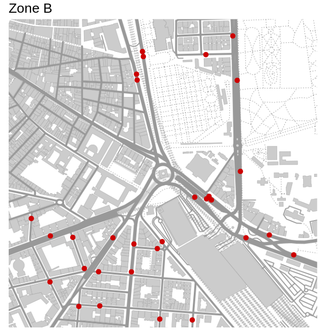
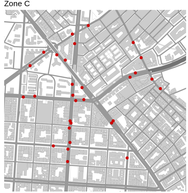
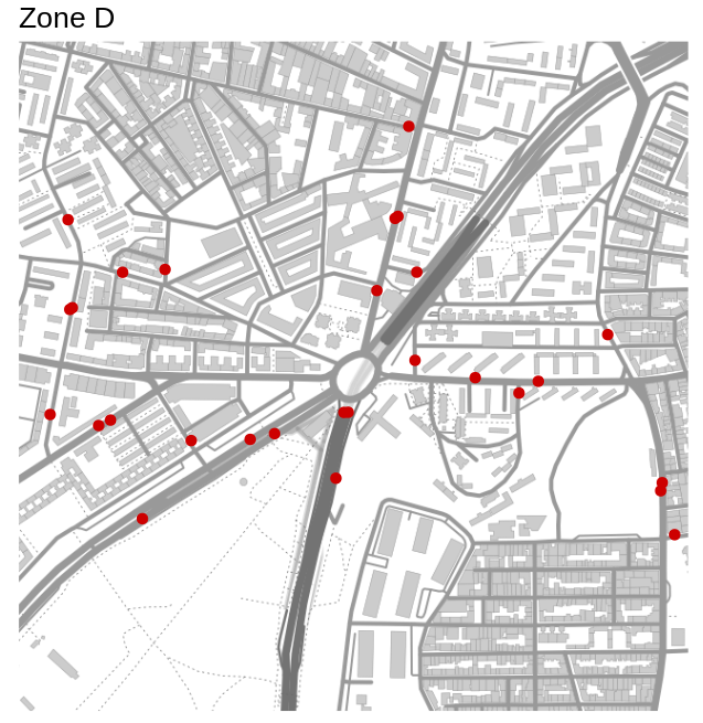
Figure 4: Location of traffic sensors for each zone.

Zone	Name	Longitude	Latitude	Mean	Std
A	Legazpi	-3.6952	40.3911	563.6	803.2
B	Atocha	-3.6920	40.4087	680.9	769.7
C	Avenida de América	-3.6774	40.4374	459.3	476.6
D	Plaza Elíptica	-3.7176	40.3852	360.2	517.8

TABLE I: Location of the center of spatial zones and name correspondence from now on. Main data statistics.

Missing values are scarce (about 1$\%$ per series). They are replaced by sensor, hour and day of the week aggregation as interpolation and closeness replacement leads to greater loss of information. Outliers represents less than $0.001\%$ of each series and are given by public events (for example, Champions League final or Basketball World Cup). As these kind of events are not representative of our problem, and thus they are excluded from our analysis.

The data are aggregated into 1-hour intervals and, due to the lack of outliers, normalized using a min-max technique to the range [0,1]. Normalization constants are calculated over the training dataset. Each spatio-temporal series is normalized separately as we are looking for an agnostic scale for each sensor.

In order to better understand our problem, we show significant properties of the data. Due to high number of sensors and the spatial heterogeneity commented above, instead of showing general attributes from our series (as mean, median or dispersion) it is more instructive to see both spatial and temporal distributions. Thus, in one hand, Fig. 5 shows a boxplot for different time variables. From this figure, it should be clear that traffic is highly dependent of time and periods of human activity. On the other hand, the spatial distribution of our series is displayed in Fig. 6. This last figure not only let us better understand our data, but also reinforces the idea of having very diverse spatial zones for our study.

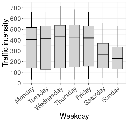
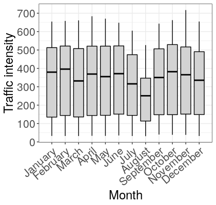
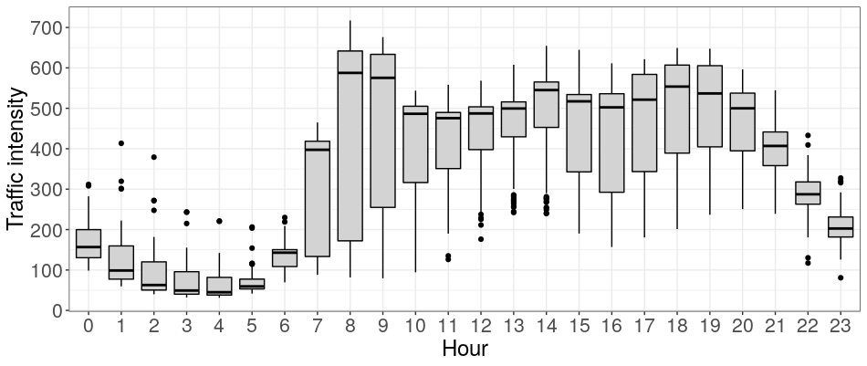
Figure 5: Hourly, weekly and monthly distribution of traffic intensity series.

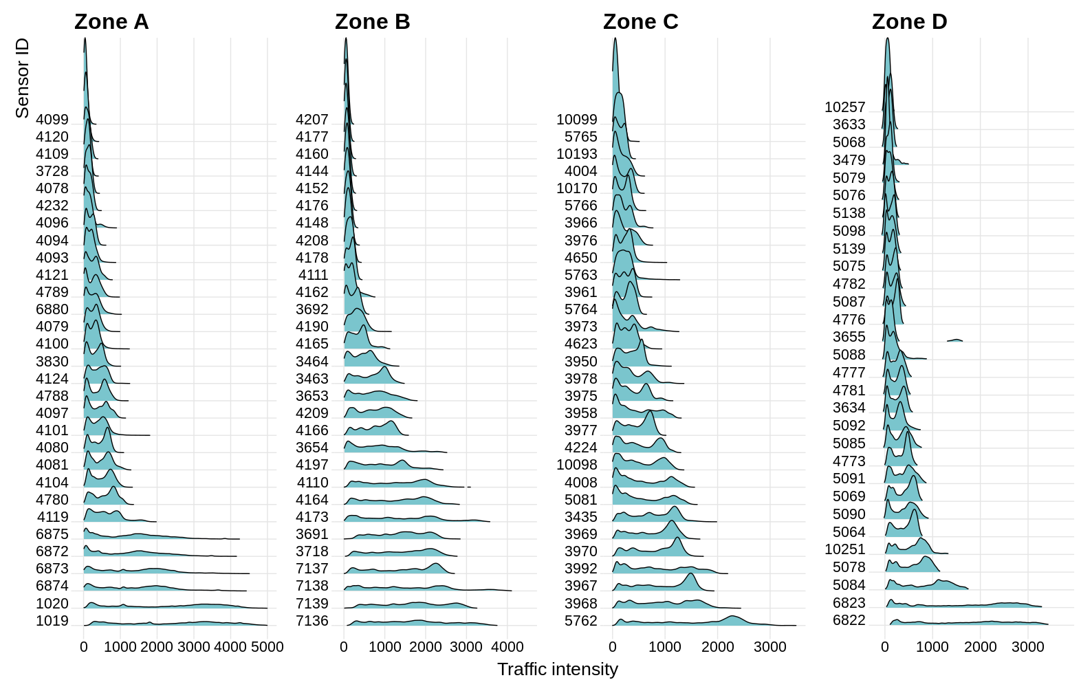
Figure 6: Traffic intensity distribution by sensor (in number of vehicles per hour).

IV-B Benchmark models

We compare the performance of the proposed CRANN with a CNN, an LSTM, the usual combination CNN+LSTM and a sequence to sequence model (seq2seq).

• CNN: A 2D convolutional model in which every channel corresponds to a timestep. The architecture consists of a sequence of convolutional layers, batch normalization and ReLU activation. For every layer a kernel size of 3 for each dimension is used. It uses 24 hours as input and outputs a 24 hours prediction.

• LSTM: These models have several hidden layers with a number of hidden units to determine. We used the $\tanh$ activation functions as in the original model. The number of inputs and outputs are equivalent to the number of sensors. Although GRUs modules have also been tested, no difference has been reported. It uses historical data from two weeks as input and outputs a 24-hour prediction.

• CNN+LSTM: A stacked model consisting of a CNN module whose output is in turn the input of a LSTM. Both modules are defined as the two previous models. It uses 24 hours as input and outputs a 24-hour prediction.

• seq2seq: These architectures are based on an encoder and a decoder, both LSTMs, without “bottleneck”. That is to say, hidden variables from all timesteps are used as inputs for the decoder. The number of inputs and outputs are equivalent to the number of sensors. As with LSTMs, GRUs did not show a better performance. It uses two weeks as input and outputs a 24 hours prediction.

With these models and their implementation particularities (inputs and outputs) we aim to cover a wide range of neural network paradigms for our comparison. For instance, CNN are specially designed for learning spatial relations, LSTMs and Seq2Seq models are designed to explore mainly time interactions and CNN+LSTM are closer to our model being a mixture of both previous approaches.

Concerning hyperparametrization and training, instead of using preset architectures, to be fair, the optimal configuration for each model was obtained via Bayesian hyperparameter optimization [57] which is defined as: building a probability model of the objective function and using it to select the most promising hyperparameters to evaluate in the true objective function. Unlike grid search and random search, the bayesian approach keeps track of past evaluation results. Final hyperparameters can be found in table II.

model	hyperparameter	value	# parameters
CNN	Convolutions	(32,32,32,64,64,64)	132k
LSTM	Number of layers	2	206k
	Hidden units	100
CNN+LSTM	Convolutions	(32,32,64,64,64)	329k
	Number of layers	2
	Hidden units	100
seq2seq	Number of layers	2	368k
	Hidden units	100
CRANN	Convolutions	(64,64,64,64,64)	1M
	Number of layers	1
	Hidden units	100
	Dense layers	1

TABLE II: Values used for each hyperparameter and total number of parameters.

All the models are trained using the mean squared error (MSE) as objective function with the Adam optimizer [58]. The batch size is 64, the initial learning rate is 0.01 and both early stopping and learning rate decay are implemented in order to avoid overfitting and improve performance. The experiments run in a NVIDIA RTX 2070.

IV-C Experimental design

In order to guarantee that models can be compared in a fair manner it is essential to fix the approach to error estimation, which must be shared as much as possible by all models. First of all, as stated in [59], standard $k$-cross-validation is the way to go when validating neural networks for time series if several conditions are met. Specifically, that we are modelling a stationary nonlinear process, that we can ensure that the leave-one-out estimation is a consistent estimator for our predictions and that we have serially uncorrelated errors.

While the first and the third conditions are trivially fulfilled for our problem, the second one needs to be specifically studied for the sake of avoiding data leakage. Given that we use all the possible series, even though the ones are unrepeated, it is possible to introduce prior information from the training to the test via closeness of samples (for example training a sequence whose start is at 10:00 AM and testing in a sequence whose start is at 11:00 AM from the same day i.e. one timestep forward). Due to this problem, it is not possible to create random folds and it is necessary to specify a separation border among different sets (training, validation and test).

In this concrete case, this separation takes as much timesteps as every model uses for its training. A scheme of this methodology is shown in Fig. 7. Particularly, a 10-cross-validation scheme without repetition is used for each spatial zone separately.

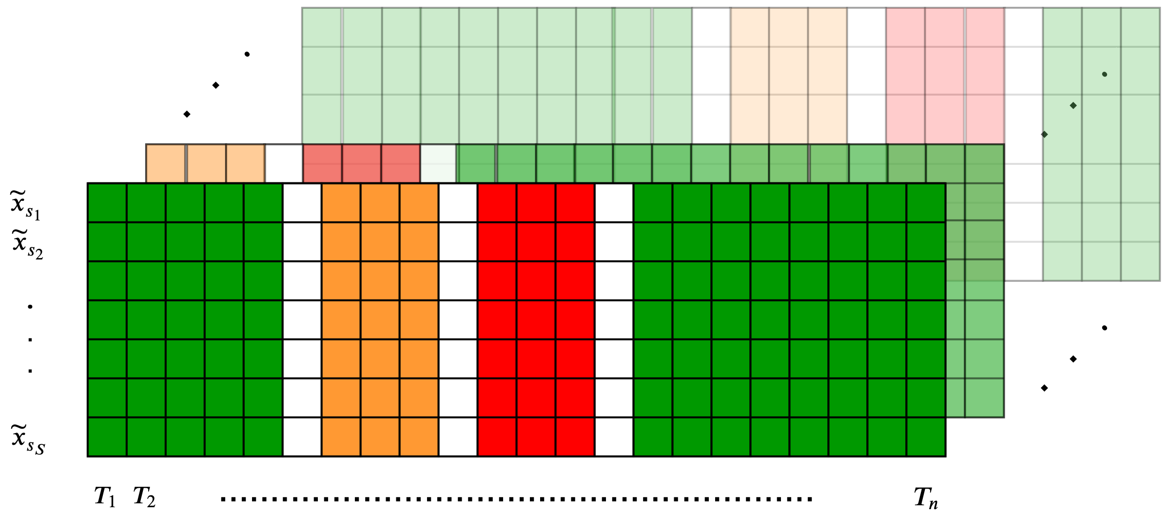
Figure 7: Validation methodology example with training (green), validation (orange) and test (red) sets for our proposed cross-validation procedure. Rows shown in white are omitted due to dependency considerations.

To evaluate the precision of each model, we computed root mean squared error (RMSE), bias and weighted mean absolute percentage error (WMAPE). In a spatio-temporal context [60], they are defined as:

$$\mathrm{RMSE}=\sqrt{\frac{1}{TS}\sum_{j=1}^{T}\sum_{i=1}^{S}(\tilde{x}_{s_{i},t_{j}}-x_{s_{i},t_{j}})^{2}},$$ (10)

$$\mathrm{bias}=\frac{1}{TS}\sum_{j=1}^{T}\sum_{i=1}^{S}(\tilde{x}_{s_{i},t_{j}}-x_{s_{i},t_{j}}),$$ (11)

$$\mathrm{WMAPE}=100\times\frac{\sum_{j=1}^{T}\sum_{i=1}^{S}\mid\tilde{x}_{s_{i},t_{j}}-x_{s_{i},t_{j}}\mid}{\sum_{j=1}^{T}\sum_{i=1}^{S}\mid x_{s_{i},t_{j}}\mid},$$ (12)

where (as in Section III-A) ${x_{s_{i},t_{j}}:j=1,...,T;i=1,...,S}$ is a spatio-temporal sample from the real series, $\tilde{x}_{s_{i},t_{j}}$ represents the predicted series, $S$ is the total number of traffic sensors and $T$ the total number of predicted timesteps.

For all these metrics, the closer to zero they are the better the performance is.

V Results

V-A Error estimation

A general comparison for the different error metrics can be seen in Table III. Bias is represented by its absolute value. These values correspond to averaging each metric for all spatial zones. Highlighted in bold, CRANN results shows a better performance overall for all errors.

model	RMSE	$|\mathrm{bias}|$	WMAPE	Run time (s)
CNN	$238.24$	$22.12$	$25.89$	$68$
LSTM	$255.76$	$19.58$	$27.46$	$552$
CNN+LSTM	$252.34$	$21.70$	$27.29$	$144$
Seq2Seq	$246.45$	$19.14$	$25.79$	$1098$
CRANN	$\mathbf{221.31}$	$\mathbf{17.80}$	$\mathbf{23.18}$	$1083$

TABLE III: Average performance for $t=1$ to $t=24$, calculated over all spatial zones and average run time per fold. For a more detailed view of error metrics distribution, see Fig. 8.

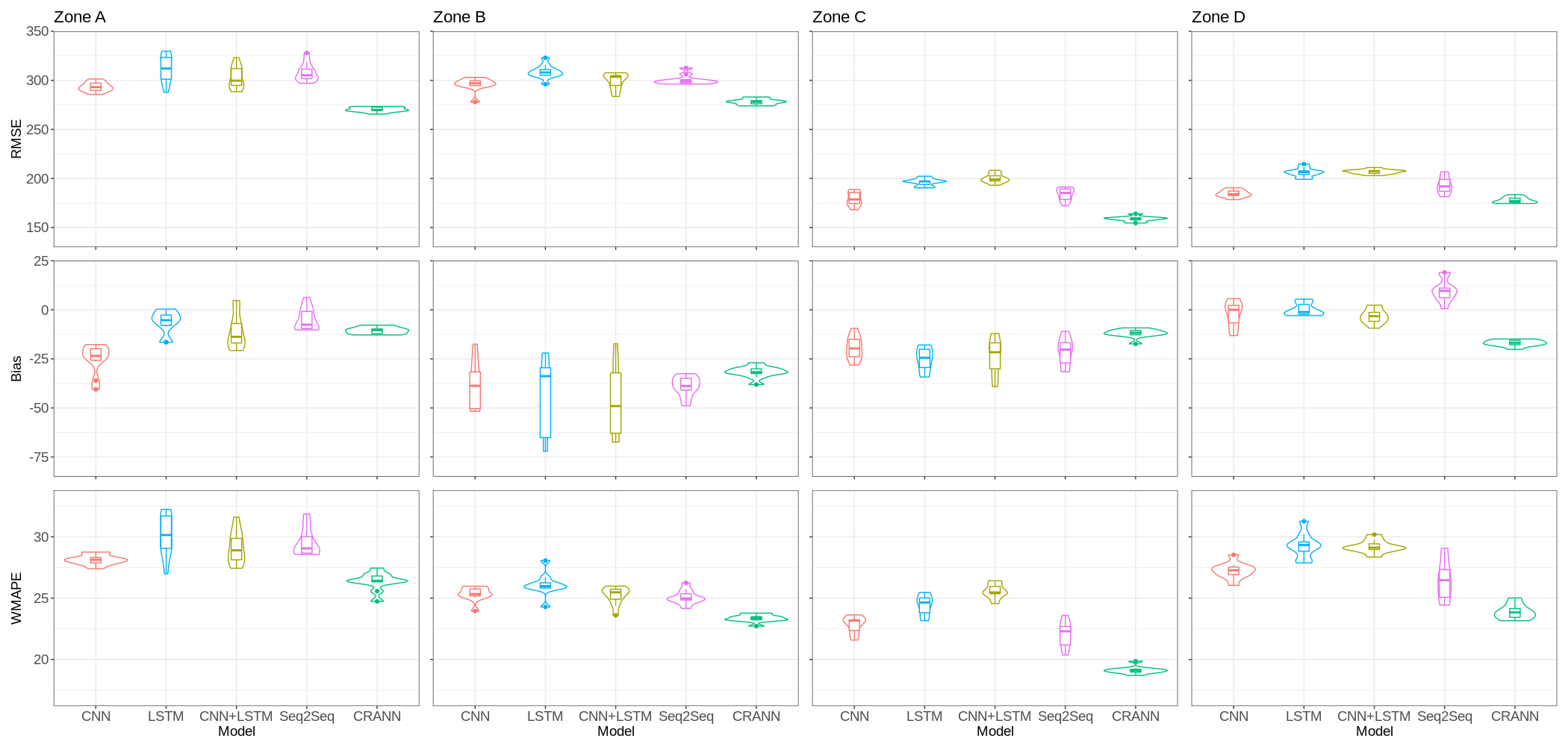
Figure 8: Violin plots of error metrics distributions for each zone and model.

For a better understanding on how each model is performing, Fig. 8 present these same error metrics but with their distribution for each zone separately. While LSTM and recurrent models in general are a standard for time series forecasting, our experiments demonstrate that standard CNN can perform similar (or even better) than recurrent models and should have a bigger space in time series. Also, vanilla LSTM might not be the best option for a real world spatio-temporal system with high complexity. Oddly, the CNN+LSTM model performs worse than the traditional CNN model, which can be due to the LSTM module negatively affecting its behaviour. With p-values $<$ 0.05 when comparing with all the baseline models, CRANN can be considered as statistically significantly better at all error metrics with a confidence of $95\%$.

From Fig 8 we can also deduce that the deviation of the CRANN model is generally stable and is the smallest one. In fact, models that are highly dependent on a recurrent neural network show a higher-deviation tendency respect to strongly CNN-based models.

Bias exhibits a clear under zero tendency, meaning that all models tend to underestimate their predictions. For a deeper understanding of this phenomenon, Fig 9 shows CRANN’s bias spatial distribution for each studied sensor. Compared with Fig 6, it is clear that traffic sensors with higher traffic intensity values, which in turn coincide with those sensors with distributions with greater dispersion, are mainly responsible of this behaviour. While we would expect higher errors in these kind of sensors with such an aggressive traffic pattern, it is not clear why the shifting occurs in only one direction. Nevertheless, as this anomaly happens for all CRANN and baseline models in every zone, we expect that its nature is intrinsic for the system or the validation methodology.

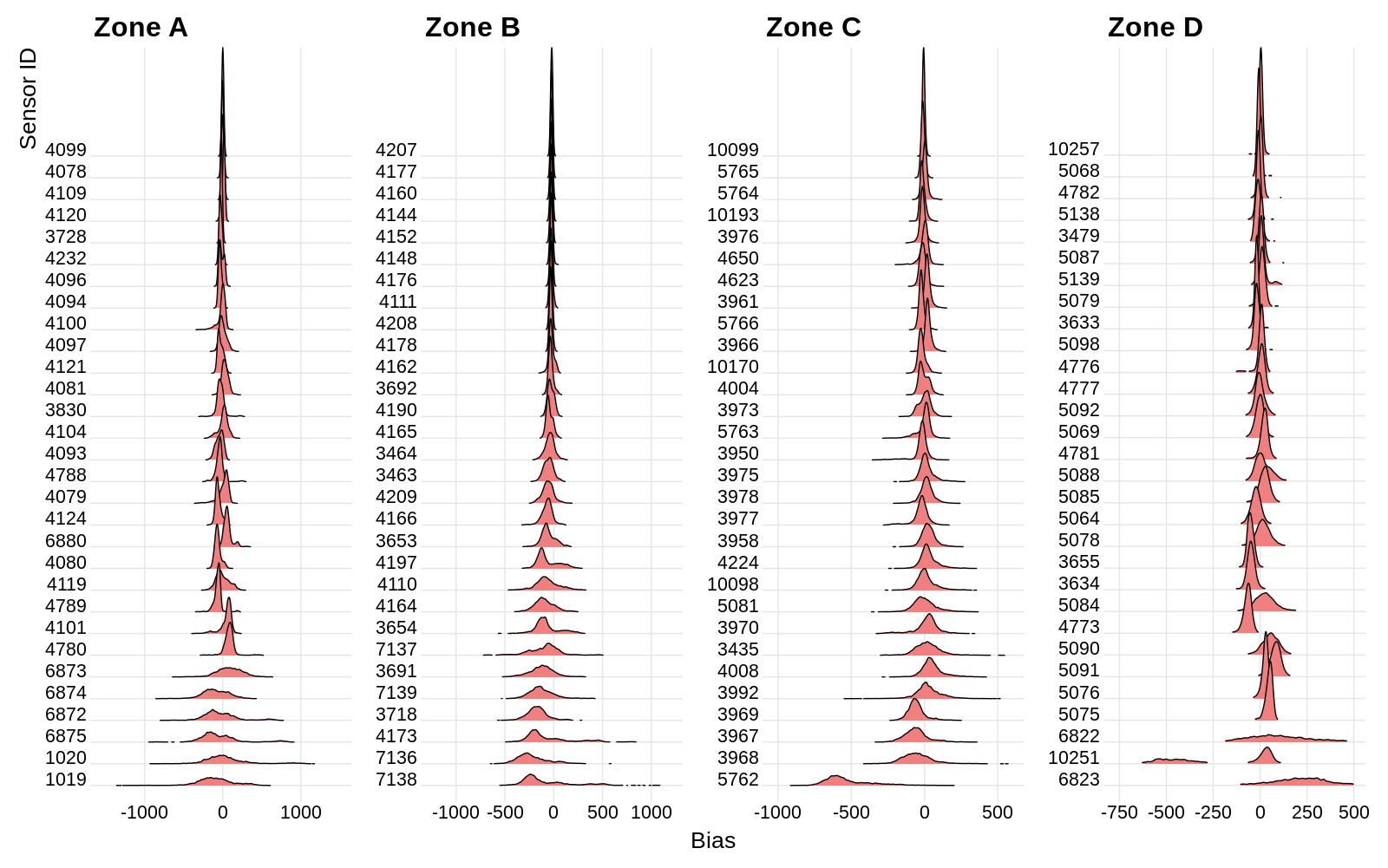
Figure 9: Bias distribution for each traffic sensor. When compared with Fig. 6 it should be clear that measurement points with higher traffic intensities and more variability are shifted to the left in bias, resulting in a underestimation of the real series.

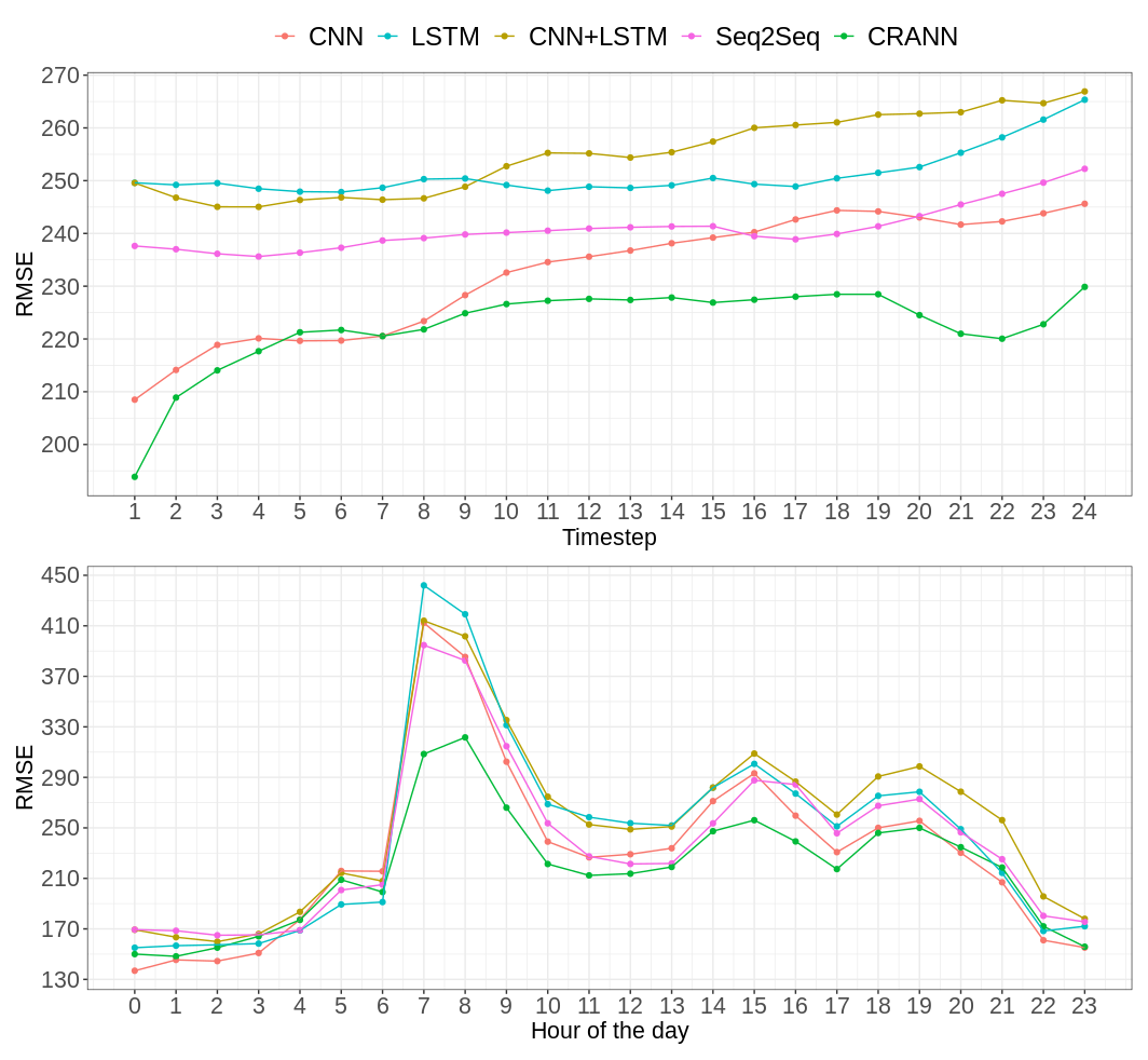
Figure 10: RMSE analysis for time dimension. How it varies depending on the prediction timestep for all models (top). Average error depending on the our of the day (bottom).

With respect to time dimension, a simple analysis can show some expected behaviour. As shown in Fig. 10 (top), all models experiment an increase of average RMSE when the predicted timestep goes further, as we could expect. As spot-forecasting is based on evaluation through all possible series, these timesteps do not have a direct correspondence with specific hours of the day and this figure is not contaminated by natural dynamics of traffic.However, there are two clear patterns: LSTM-based models (LSTM, CNN+LSTM and seq2seq) share a higher error for the first horizons, which are usually considered easier to predict under the hipothesis of inertia of the series. This tells us that they are not capturing this inertia correctly. At the same time, CNN-based models (CNN and CRANN) manage to capture the inertia of the series. Having introduced autoregressive terms into the CRANN model stands as a positive alternative to alleviate and improve this difficulty. Also, we can see a valley from timestep $t+20$ to $t+24$ as due to traffic periodicity, that fraction of the series is highly similar to the one introduced as autoregressive terms (timesteps $t-1$ to $t-4$).

Meanwhile, Fig. 10 (bottom) let us understand how the average error of the different models are distributed as a function of the hour of the day in which the prediction is being made. As we would expect, these errors are bigger at rush hours, giving us a distribution with same shape than the one presented in Fig. 5. Nevertheless, CRANN model stands out for its ability to outperform significantly its rivals in those exact instants, when it is precisely more useful and challenging to get a good behavior.

Figure 11: Example of CRANN’s predictions for all zones. Average results for predictions starting at 00:00 and ending at 23:00.

Lastly, Fig. 11 displays an example forecast of CRANN. By taking all series starting at 00:00 and ending at 23:00 it is possible to visualize average performance of the model in a specific context. This figure clearly shows how our model is successfull in learning the spatio-temporal dynamic of traffic, even adapting its behaviour to fine details in a highly complex spatio-temporal problem.

V-B Interpretability

In order to better understand how our model works, we might use all the interpretability layers presented in Section III-B4. Also, interpretability will let us corroborate our initial hypothesis about how each module tackles different aspect of spatio-temporal series: trend, seasonality, inertia and spatial relations.

Starting by our temporal module (see Sec. III-B2), Fig. 12 shows average attention weights computed by the attention mechanism in function of both input and output timesteps. From this figure we can have a clear intuition about the 24 hour pattern that our model has learned. At the same time, time-back steps $~{}160$ and $~{}325$, which correspond to 7 and 14 days before the prediction, show to be more important as traffic presents a seven days seasonality too. As the input series approach to the forecasting window, the importance keeps growing proving that the temporal module is regulating trend as we were looking for. The fact that no shifting is happening is due to averaging over all test samples.

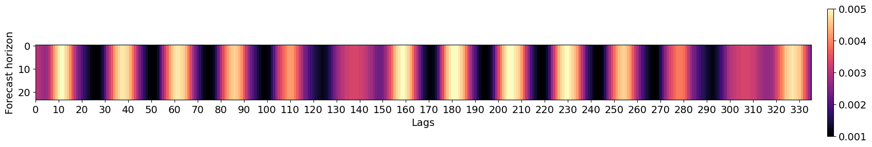
Figure 12: Average temporal attention given by the temporal module of CRANN. Attention weights are represented as a function of input and output series. In the x-axis, past lags from the input series. In the y-axis, forecast horizons (i.e. future lags) from the output series. A $(x,y)$ value represents how important is timestep $x$ to predict timestep $y$.

With respect to the spatial module attention (see Sect. III-B3), it is obviously highly dependent on each specific zone. For that reason, Fig. 13 illustrates the attention weights for traffic sensors in Zone D. As our defined spatial attention mechanism uses different weights for each lag of the input, average values are shown. As it can be seen (top), sensors with specially complex conditions (high traffic intensity, big avenues…) are usually scored as more important by the spatio-temporal attention mechanism. This is the case of points 8, 27 and 28 for example. On the contrary, those points that we would expect to have less impact in global traffic show smaller values, like sensors 4, 16 and 20. Similarly (bottom), sensors in heavy traffic intensity emplacements show to receive higher attention. As we tackle the long-term forecasting problem, we do not expect our model to pay attention by closeness, but by general importance in the entire zone.

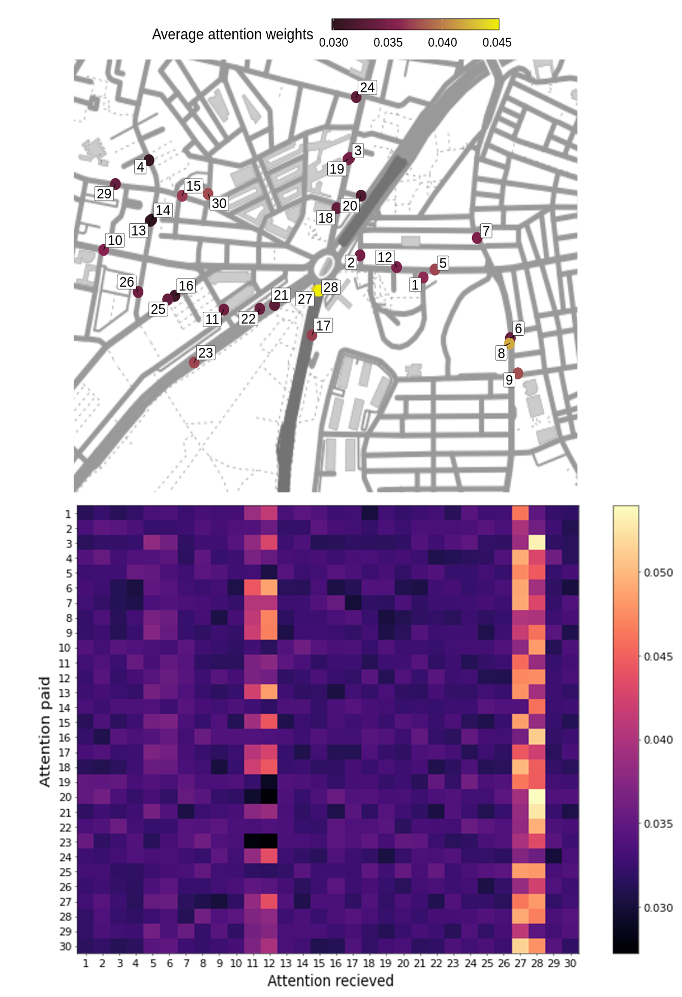
Figure 13: Average spatial attention given by CRANN spatial module at zone D. Attention weights are averaged for all sensors and timesteps (top). Attention weights for each pair of sensors (bottom).

Finally, from average SHAP values computed for the dense module at Zone D (see Sect. III-B4), shown in Fig. 14, we can extract several conclusions. First of all, it supports the idea that using average traffic intensity (“Mean”) for trend and seasonality modelling (temporal module) might be beneficial. Secondly, the importance given to traffic sensors follow a similar pattern to the one seen previously by the spatio-temporal attention mechanism, reinforcing the idea of which spatial points are more important. Thirdly, the autoregresive term that tries to capture the intertia of the series seems to contribute positively too. Lastly, exogenous data importance points out that it has the ability of improving the prediction significantly and should be chosen carefully for each problem.

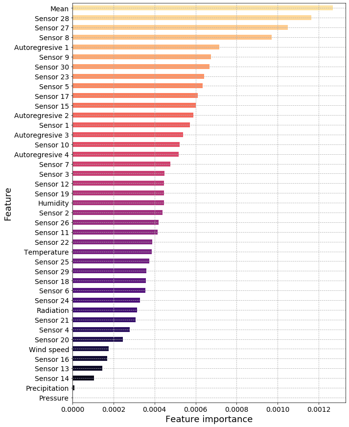
Figure 14: Mean SHAP values for all features in dense module computed in zone D. Temporal module output (Mean), spatial module output (Sensors), autoregresive terms and exogenous variables (both represented by their names).

VI Conclusions and future directions

Through this paper, a new spatio-temporal framework based on attention mechanisms whose operation rest on several spatio-temporal series components is presented. Unlike previous methodologies, we focus our efforts in creating a system that can be considered robust and adaptable, evaluating it in a non-fixed scenario. After being applied to a real traffic dataset, it has been proved that outperforms four state of the art neural architectures and it has been studied its behaviour respect to both time and spatial dimension through extensive experimentation. By analyzing four different locations with 30 traffic sensors each, we can confirm the statistical significance of our results with a confidence of $95\%$ for forecasting horizons of up to 24 hours.

Thanks to the interpretable nature of the model, we have illustrated how that information might be used in order to understand better how the framework works, how it can give us specific information from the problem domain and why our network architecture is well founded. Concretely, the conducted experiments have shown that, as we postulated, the temporal module regulates seasonality and trend, spatial module is capable of extracting short-term and spatial relations, and that it is necessary to introduce explicit autoregressive terms in order to exploit inertia correctly. Finally, these experiments demonstrate the effectiveness of all these terms to make the final prediction.

For future work, it might be interesting to evaluate the proposed method over a wider range of series in order to generalize the results and see its behaviour over different applications. With the actual ability from the spatial module to model attention for both input dimensions, space and time, it could be beneficial to extend these idea to outputs dimensions too, having different attention weights for different predicted timesteps. Lastly, it should be studied how to use exogenous spatio-dependent data in the best possible way.

VII Acknowledgements

This research has been partially funded by the Empresa Municipal de Transportes (EMT) of Madrid under the program ”Aula Universitaria EMT/UNED de Calidad del Aire y Movilidad Sostenible”.

References

- [1] “Digital Earth,” library Catalog: www.digitalearth.art. [Online]. Available: https://www.digitalearth.art
- [2] “Galileo is the European global satellite-based navigation system | European Global Navigation Satellite Systems Agency.” [Online]. Available: https://www.gsa.europa.eu/european-gnss/galileo/galileo-european-global-satellite-based-navigation-system
- [3] Y. Wang, M. Long, J. Wang, Z. Gao, and P. S. Yu, “PredRNN: Recurrent Neural Networks for Predictive Learning using Spatiotemporal LSTMs,” in Advances in Neural Information Processing Systems 30, I. Guyon, U. V. Luxburg, S. Bengio, H. Wallach, R. Fergus, S. Vishwanathan, and R. Garnett, Eds. Curran Associates, Inc., 2017, pp. 879–888.
- [4] A. Alahi, K. Goel, V. Ramanathan, A. Robicquet, L. Fei-Fei, and S. Savarese, “Social LSTM: Human Trajectory Prediction in Crowded Spaces,” in 2016 IEEE Conference on Computer Vision and Pattern Recognition (CVPR), Jun. 2016, pp. 961–971, iSSN: 1063-6919.
- [5] Q. Tang, M. Yang, and Y. Yang, “ST-LSTM: A Deep Learning Approach Combined Spatio-Temporal Features for Short-Term Forecast in Rail Transit,” 2019, iSSN: 0197-6729 Library Catalog: www.hindawi.com Pages: e8392592 Publisher: Hindawi Volume: 2019.
- [6] J. Ke, H. Yang, H. Zheng, X. Chen, Y. Jia, P. Gong, and J. Ye, “Hexagon-Based Convolutional Neural Network for Supply-Demand Forecasting of Ride-Sourcing Services,” IEEE Transactions on Intelligent Transportation Systems, vol. 20, no. 11, pp. 4160–4173, Nov. 2019, conference Name: IEEE Transactions on Intelligent Transportation Systems.
- [7] L. Duan, T. Hu, E. Cheng, J. Zhu, and C. Gao, “Deep Convolutional Neural Networks for Spatiotemporal Crime Prediction,” p. 7.
- [8] Q. Zhu, J. Chen, L. Zhu, X. Duan, and Y. Liu, “Wind Speed Prediction with Spatio–Temporal Correlation: A Deep Learning Approach,” Energies, vol. 11, no. 4, p. 705, Apr. 2018, number: 4 Publisher: Multidisciplinary Digital Publishing Institute.
- [9] B. Liao, F. Wu, J. Zhang, M. Cai, S. Tang, Y. Gao, C. Wu, S. Yang, W. Zhu, and Y. Guo, “Dest-ResNet: A Deep Spatiotemporal Residual Network for Hotspot Traffic Speed Prediction,” in 2018 ACM Multimedia Conference on Multimedia Conference - MM ’18. Seoul, Republic of Korea: ACM Press, 2018, pp. 1883–1891.
- [10] B. Liao, J. Zhang, C. Wu, D. McIlwraith, T. Chen, S. Yang, Y. Guo, and F. Wu, “Deep Sequence Learning with Auxiliary Information for Traffic Prediction,” in Proceedings of the 24th ACM SIGKDD International Conference on Knowledge Discovery & Data Mining, ser. KDD ’18. London, United Kingdom: Association for Computing Machinery, Jul. 2018, pp. 537–546.
- [11] H.-F. Yang, T. S. Dillon, and Y.-P. P. Chen, “Optimized Structure of the Traffic Flow Forecasting Model With a Deep Learning Approach,” IEEE Transactions on Neural Networks and Learning Systems, vol. 28, no. 10, pp. 2371–2381, Oct. 2017, conference Name: IEEE Transactions on Neural Networks and Learning Systems.
- [12] M.-T. Luong, H. Pham, and C. D. Manning, “Effective Approaches to Attention-based Neural Machine Translation,” arXiv:1508.04025 [cs], Sep. 2015, arXiv: 1508.04025.
- [13] D. Bahdanau, K. Cho, and Y. Bengio, “Neural Machine Translation by Jointly Learning to Align and Translate,” arXiv:1409.0473 [cs, stat], May 2016, arXiv: 1409.0473.
- [14] W. Cheng, Y. Shen, Y. Zhu, and L. Huang, “A neural attention model for urban air quality inference: Learning the weights of monitoring stations,” in Proceedings of the Thirty-Second AAAI Conference on Artificial Intelligence, (AAAI-18), the 30th innovative Applications of Artificial Intelligence (IAAI-18), and the 8th AAAI Symposium on Educational Advances in Artificial Intelligence (EAAI-18), New Orleans, Louisiana, USA, February 2-7, 2018, S. A. McIlraith and K. Q. Weinberger, Eds. AAAI Press, 2018, pp. 2151–2158.
- [15] Y. Chen, G. Peng, Z. Zhu, and S. Li, “A novel deep learning method based on attention mechanism for bearing remaining useful life prediction,” Applied Soft Computing, vol. 86, p. 105919, Jan. 2020.
- [16] X. Fu, F. Gao, J. Wu, X. Wei, and F. Duan, “Spatiotemporal Attention Networks for Wind Power Forecasting,” arXiv:1909.07369 [cs], Sep. 2019, arXiv: 1909.07369.
- [17] S. Wang, J. Cao, and P. S. Yu, “Deep Learning for Spatio-Temporal Data Mining: A Survey,” arXiv:1906.04928 [cs, stat], Jun. 2019, arXiv: 1906.04928.
- [18] Hamed Mohammad M., Al-Masaeid Hashem R., and Said Zahi M. Bani, “Short-Term Prediction of Traffic Volume in Urban Arterials,” Journal of Transportation Engineering, vol. 121, no. 3, pp. 249–254, May 1995, publisher: American Society of Civil Engineers.
- [19] M. V. D. Voort, M. Dougherty, and S. Watson, “Combining kohonen maps with arima time series models to forecast traffic flow,” Transportation Research Part C: Emerging Technologies, vol. 4, no. 5, pp. 307 – 318, 1996.
- [20] S. V. Kumar and L. Vanajakshi, “Short-term traffic flow prediction using seasonal ARIMA model with limited input data,” European Transport Research Review, vol. 7, no. 3, p. 21, Jun. 2015.
- [21] S. Sun, C. Zhang, and Y. Zhang, “Traffic Flow Forecasting Using a Spatio-temporal Bayesian Network Predictor,” p. 6.
- [22] C. M. Queen and C. J. Albers, “Intervention and Causality: Forecasting Traffic Flows Using a Dynamic Bayesian Network,” Journal of the American Statistical Association, vol. 104, no. 486, pp. 669–681, Jun. 2009.
- [23] A. Pascale and M. Nicoli, 2011 IEEE Statistical Signal Processing Workshop (SSP) ADAPTIVE BAYESIAN NETWORK FOR TRAFFIC FLOW PREDICTION.
- [24] X. Dong, T. Lei, S. Jin, and Z. Hou, “Short-Term Traffic Flow Prediction Based on XGBoost,” in 2018 IEEE 7th Data Driven Control and Learning Systems Conference (DDCLS). Enshi: IEEE, May 2018, pp. 854–859.
- [25] W. Alajali, W. Zhou, S. Wen, and Y. Wang, “Intersection Traffic Prediction Using Decision Tree Models,” Symmetry, vol. 10, no. 9, p. 386, Sep. 2018.
- [26] W. Alajali, W. Zhou, and S. Wen, “Traffic Flow Prediction for Road Intersection Safety,” in 2018 IEEE SmartWorld, Ubiquitous Intelligence & Computing, Advanced & Trusted Computing, Scalable Computing & Communications, Cloud & Big Data Computing, Internet of People and Smart City Innovation (SmartWorld/SCALCOM/UIC/ATC/CBDCom/IOP/SCI). Guangzhou, China: IEEE, Oct. 2018, pp. 812–820.
- [27] T. Wu, K. Xie, G. Song, and C. Hu, “A Multiple SVR Approach with Time Lags for Traffic Flow Prediction,” in 2008 11th International IEEE Conference on Intelligent Transportation Systems, Oct. 2008, pp. 228–233, iSSN: 2153-0009, 2153-0017.
- [28] Y. Cong, J. Wang, and X. Li, “Traffic Flow Forecasting by a Least Squares Support Vector Machine with a Fruit Fly Optimization Algorithm,” Procedia Engineering, vol. 137, pp. 59–68, Jan. 2016.
- [29] Z. Mingheng, Z. Yaobao, H. Ganglong, and C. Gang, “Accurate Multisteps Traffic Flow Prediction Based on SVM,” 2013.
- [30] Z. Liu, Z. Li, K. Wu, and M. Li, “Urban Traffic Prediction from Mobility Data Using Deep Learning,” IEEE Network, vol. 32, no. 4, pp. 40–46, Jul. 2018.
- [31] A. Ermagun and D. Levinson, “Spatiotemporal traffic forecasting: review and proposed directions,” Transport Reviews, vol. 38, no. 6, pp. 786–814, Nov. 2018.
- [32] Y. Wu, H. Tan, L. Qin, B. Ran, and Z. Jiang, “A hybrid deep learning based traffic flow prediction method and its understanding,” Transportation Research Part C: Emerging Technologies, vol. 90, pp. 166–180, May 2018.
- [33] L. N. N. Do, H. L. Vu, B. Q. Vo, Z. Liu, and D. Phung, “An effective spatial-temporal attention based neural network for traffic flow prediction,” Transportation Research Part C: Emerging Technologies, vol. 108, pp. 12–28, Nov. 2019.
- [34] S. Guo, Y. Lin, S. Li, Z. Chen, and H. Wan, “Deep Spatial–Temporal 3d Convolutional Neural Networks for Traffic Data Forecasting,” IEEE Transactions on Intelligent Transportation Systems, vol. 20, no. 10, pp. 3913–3926, Oct. 2019.
- [35] T. Bogaerts, A. D. Masegosa, J. S. Angarita-Zapata, E. Onieva, and P. Hellinckx, “A graph CNN-LSTM neural network for short and long-term traffic forecasting based on trajectory data,” Transportation Research Part C: Emerging Technologies, vol. 112, pp. 62–77, Mar. 2020.
- [36] S. Deng, S. Jia, and J. Chen, “Exploring spatial–temporal relations via deep convolutional neural networks for traffic flow prediction with incomplete data,” Applied Soft Computing, vol. 78, pp. 712–721, May 2019.
- [37] L. Qu, W. Li, W. Li, D. Ma, and Y. Wang, “Daily long-term traffic flow forecasting based on a deep neural network,” Expert Systems with Applications, vol. 121, pp. 304–312, May 2019.
- [38] Z. He, C.-Y. Chow, and J.-D. Zhang, “STCNN: A Spatio-Temporal Convolutional Neural Network for Long-Term Traffic Prediction,” in 2019 20th IEEE International Conference on Mobile Data Management (MDM), Jun. 2019, pp. 226–233, iSSN: 1551-6245.
- [39] C. Bergmeir, R. Hyndman, and J. Benítez, “Bagging exponential smoothing methods using STL decomposition and Box–Cox transformation,” International Journal of Forecasting, vol. 32, no. 2, pp. 303–312, Apr. 2016.
- [40] E. M. de Oliveira and F. L. Cyrino Oliveira, “Forecasting mid-long term electric energy consumption through bagging ARIMA and exponential smoothing methods,” Energy, vol. 144, pp. 776–788, Feb. 2018.
- [41] Z. Li, Y. Li, and L. Li, “A comparison of detrending models and multi-regime models for traffic flow prediction,” IEEE Intelligent Transportation Systems Magazine, vol. 6, no. 4, pp. 34–44, 2014.
- [42] X. Dai, R. Fu, Y. Lin, L. Li, and F.-Y. Wang, “DeepTrend: A Deep Hierarchical Neural Network for Traffic Flow Prediction,” arXiv:1707.03213 [cs], Jul. 2017, arXiv: 1707.03213.
- [43] X. Dai, R. Fu, E. Zhao, Z. Zhang, Y. Lin, F.-Y. Wang, and L. Li, “DeepTrend 2.0: A light-weighted multi-scale traffic prediction model using detrending,” Transportation Research Part C: Emerging Technologies, vol. 103, pp. 142–157, Jun. 2019.
- [44] G. Lai, W.-C. Chang, Y. Yang, and H. Liu, “Modeling Long- and Short-Term Temporal Patterns with Deep Neural Networks,” arXiv:1703.07015 [cs], Apr. 2018, arXiv: 1703.07015.
- [45] B. Liu, X. Tang, J. Cheng, and P. Shi, “Traffic Flow Combination Forecasting Method Based on Improved LSTM and ARIMA,” p. 8.
- [46] K. Bandara, C. Bergmeir, and H. Hewamalage, “LSTM-MSNet: Leveraging Forecasts on Sets of Related Time Series with Multiple Seasonal Patterns,” arXiv:1909.04293 [cs, stat], Sep. 2019, arXiv: 1909.04293.
- [47] S. B. Taieb, G. Bontempi, A. F. Atiya, and A. Sorjamaa, “A review and comparison of strategies for multi-step ahead time series forecasting based on the nn5 forecasting competition,” Expert Systems with Applications, vol. 39, no. 8, pp. 7067 – 7083, 2012.
- [48] M. Nelson, T. Hill, W. Remus, and M. O’Connor, “Time series forecasting using neural networks: should the data be deseasonalized first?” Journal of Forecasting, vol. 18, no. 5, pp. 359–367, 1999.
- [49] O. Li, H. Liu, C. Chen, and C. Rudin, “Deep Learning for Case-Based Reasoning through Prototypes: A Neural Network that Explains Its Predictions,” p. 8.
- [50] Q. You, H. Jin, Z. Wang, C. Fang, and J. Luo, “Image captioning with semantic attention,” in The IEEE Conference on Computer Vision and Pattern Recognition (CVPR), June 2016.
- [51] J. Wang, R. Chen, and Z. He, “Traffic speed prediction for urban transportation network: A path based deep learning approach,” Transportation Research Part C: Emerging Technologies, vol. 100, pp. 372 – 385, 2019.
- [52] Z. Cui, K. Henrickson, R. Ke, X. Dong, and Y. Wang, “High-Order Graph Convolutional Recurrent Neural Network: A Deep Learning Framework for Network-Scale Traffic Learning and Forecasting,” 2019, number: 19-05236.
- [53] K. Cho, B. van Merriënboer, D. Bahdanau, and Y. Bengio, “On the properties of neural machine translation: Encoder–decoder approaches,” in Proceedings of SSST-8, Eighth Workshop on Syntax, Semantics and Structure in Statistical Translation. Doha, Qatar: Association for Computational Linguistics, Oct. 2014, pp. 103–111.
- [54] X. Glorot and Y. Bengio, “Understanding the difficulty of training deep feedforward neural networks,” p. 8.
- [55] M. Sundararajan, A. Taly, and Q. Yan, “Axiomatic attribution for deep networks,” in Proceedings of the 34th International Conference on Machine Learning-Volume 70. JMLR. org, 2017, pp. 3319–3328.
- [56] S. M. Lundberg and S.-I. Lee, “A unified approach to interpreting model predictions,” in Advances in neural information processing systems, 2017, pp. 4765–4774.
- [57] J. Wu, X.-Y. Chen, H. Zhang, L.-D. Xiong, H. Lei, and S.-H. Deng, “Hyperparameter Optimization for Machine Learning Models Based on Bayesian Optimizationb,” Journal of Electronic Science and Technology, vol. 17, no. 1, pp. 26–40, Mar. 2019.
- [58] D. P. Kingma and J. Ba, “Adam: A Method for Stochastic Optimization,” ICLR 2015, Jan. 2017, arXiv: 1412.6980.
- [59] C. Bergmeir, R. J. Hyndman, and B. Koo, “A note on the validity of cross-validation for evaluating autoregressive time series prediction,” Computational Statistics & Data Analysis, vol. 120, pp. 70–83, Apr. 2018.
- [60] C. K. Wikle, A. Zammit-Mangion, and N. Cressie, Spatio-Temporal Statistics with R, 1st ed. Boca Raton, Florida : CRC Press, [2019]: Chapman and Hall/CRC, Feb. 2019. [Online]. Available: https://www.taylorfrancis.com/books/9780429649783