Effects of social distancing and isolation on epidemic spreading: a dynamical density functional theory model

Abstract

For preventing the spread of epidemics such as the coronavirus disease COVID-19, social distancing and the isolation of infected persons are crucial. However, existing reaction-diffusion equations for epidemic spreading are incapable of describing these effects. We present an extended model for disease spread based on combining an SIR model with a dynamical density functional theory where social distancing and isolation of infected persons are explicitly taken into account. The model shows interesting nonequilibrium phase separation associated with a reduction of the number of infections, and allows for new insights into the control of pandemics.

I Introduction

Controlling the spread of infectious diseases, such as the plague Poland and Dennis (1998) or the Spanish flu Wilton (1993), has been an important topic throughout human history Cliff and Smallman-Raynor (2013). Currently, it is of particular interest due to the worldwide outbreak of the coronavirus disease 2019 (COVID-19) induced by the novel coronavirus SARS-CoV-2 Wu et al. (2020); Zhou et al. (2020); Cui et al. (2019); Wang et al. (2020). The spread of this disease is difficult to control, since the majority of infections are not detected Li et al. (2020). Due to the lack of vaccines, attempts to control the pandemic have mainly focused on social distancing Stein (2020); Ferguson et al. (2020) and quarantine Mizumoto and Chowell (2020); Lau et al. (2020), i.e., the general reduction of social interactions, and in particular the isolation of persons with actual or suspected infection. While political decisions on such measures require a way for predicting their effects, existing theories do not explicitly take them into account.

In this article, we present a dynamical density functional theory (DDFT) Marini Bettolo Marconi and Tarazona (1999); Archer and Evans (2004) for epidemic spreading that allows to model the effect of social distancing and isolation on infection numbers. Our model is based on combining the general idea of a reaction-diffusion DDFT from soft matter physics with the SIR model from theoretical biology. The phase diagram predicted by our model shows that, at parameter values corresponding to certain strengths and ratios of social distancing and self-isolation, the system undergoes a phase transition to a state where the spread of the pandemic is suppressed. For all regions of the phase diagram, the predicted curves have the shape that is observed in real pandemics. Numerically, the inhibition of epidemic spreading is found to be associated with nonequilibrium phase separation, where infected persons accumulate at certain spots (“leper colonies”). Our results are of high interest for the control of pandemics, since the effects of social distancing and the properties of the disease can be studied separately. Moreover, the observed phase separation effects can also be expected to occur in crowded (bio-)chemical systems, which are governed by similar equations.

II Results

II.1 SIR-DDFT model

A quantitative understanding of disease spreading can be gained from mathematical models Cai et al. (2015); Leventhal et al. (2015); De Domenico et al. (2016); Gómez-Gardenes et al. (2018). A well-known theory for epidemic dynamics is the SIR model Kermack and McKendrick (1927)

$$\dot{S} =-cSI,$$ (1)

$$\dot{I} =cSI-wI,$$ (2)

$$\dot{R} =wI,$$ (3)

which has already been applied to the current coronavirus outbreak Nesteruk (2020); Simha et al. (2020). It is a reaction-model that describes the number of susceptible $S$, infected $I$, and recovered $R$ individuals as a function of time $t$. Susceptible individuals get the disease when meeting infected individuals at a rate $c$. Infected persons recover from the disease at a rate $w$. When persons have recovered, they are immune to the disease.

A drawback of this model is that it describes a spatially homogeneous dynamics, i.e., it does not take into account the fact that healthy and infected persons are not distributed homogeneously in space, even though this fact can have significant influence on the pandemic Zhong et al. (2020); Wang and Wu (2018). To allow for spatial dynamics, disease-spreading theories such as the SIR model have been extended to reaction-diffusion equations Colizza et al. (2007); Postnikov and Sokolov (2007); Naether et al. (2008); Belik et al. (2011); Wang et al. (2012); Bacaër and Sokhna (2005); Peng and Liu (2009), where a term $D_{\phi}\vec{\nabla}^{2}\phi$ with diffusion constant $D_{\phi}$ is added on the right-hand side of the dynamical equation for $\phi=S,I,R$.

Reaction-diffusion equations, however, still have the problem that they – being based on the standard diffusion equation – do not take into account particle interactions other than the reactions. This issue arises, e.g., in chemical reactions in crowded environments such as inside a cell. In this case, the reactands, which are not pointlike, cannot move freely, which prevents them from meeting and thus from reacting. To get an improved model, one can make use of the fact that the diffusion equation is a special case of DDFT. In this theory, the time evolution of a density field $\rho(\vec{r},t)$ with spatial variable $\vec{r}$ is given by

$$\partial_{t}\rho=\Gamma\vec{\nabla}\cdot\bigg{(}\rho\vec{\nabla}\frac{\delta F}{\delta\rho}\bigg{)}$$ (4)

with a mobility $\Gamma$ and a free energy $F$. Note that we have written Eq. 4 without noise terms, which implies that $\rho(\vec{r},t)$ denotes an ensemble average Archer and Rauscher (2004). The free energy is given by

$$F=F_{\mathrm{id}}+F_{\mathrm{exc}}+F_{\mathrm{ext}}.$$ (5)

Its first contribution is the ideal gas free energy

$$F_{\mathrm{id}}=\beta^{-1}{\int\;\;\;\mathrm{d}^{d}r}\,\rho(\vec{r},t)(\ln(\rho(\vec{r},t)\Lambda^{d})-1),$$ (6)

corresponding to a system of noninteracting particles with the inverse temperature $\beta$, number of spatial dimensions $d$, and thermal de Broglie wavelength $\Lambda$. If this is the only contribution, Eq. 4 reduces to the standard diffusion equation with $D=\Gamma\beta^{-1}$. The second contribution is the excess free energy $F_{\mathrm{exc}}$, which takes the effect of particle interactions into account. It is typically not known exactly and has to be approximated. The third contribution $F_{\mathrm{ext}}$ incorporates the effect of an external potential $U_{\mathrm{ext}}(\vec{r},t)$. DDFT can be extended to mixtures Archer (2005); Wittkowski et al. (2012), which makes it applicable to chemical reactions. While DDFT is not an exact theory (it is based on the assumption that the density is the only slow variable in the system Español and Löwen (2009); te Vrugt and Wittkowski (2019a)), it is nevertheless a significant improvement compared to the standard diffusion equation as it allows to incorporate the effects of particle interactions and generally shows excellent agreement with microscopic simulations. In particular, it allows to incorporate the effects of particle interactions such as crowding in reaction-diffusion equations. This is done by replacing the diffusion term $D\vec{\nabla}^{2}\phi(\vec{r},t)$ in the standard reaction-diffusion model with the right-hand side of the DDFT equation (4) Lutsko (2016); Lutsko and Nicolis (2016); Liu and Liu (2020). Thus, given that its equilibrium counterpart, static density functional theory, has already been used to model crowds Méndez-Valderrama et al. (2018), DDFT is a very promising approach for the development of extended models for epidemic spreading. However, despite the successes of DDFT in other biological contexts such as cancer growth Al-Saedi et al. (2018), protein adsorption Angioletti-Uberti et al. (2018), ecology Martínez-García et al. (2013), or active matter Wensink and Löwen (2008); Wittkowski and Löwen (2011); Menzel et al. (2016); Hoell et al. (2019); Pototsky and Stark (2012); Wittmann and Brader (2016); Wittmann et al. (2017), no attempts have been made to apply DDFT to epidemic spreading (or other types of socio-economic dynamics).

We use the idea of a reaction-diffusion DDFT to extend the SIR model given by Eqs. (1)-(3) to a (probably spatially inhomogeneous) system of interacting persons, which compared to existing methods allows the incorporation of social interactions and social distancing. Persons are modelled as diffusing particles that can be susceptible to, infected with, or recovered from a certain disease. Social distancing and self-isolation are incorporated as repulsive interactions. The dynamics of the interacting particles can then be described by DDFT, while reaction terms account for disease transmission and recovery. DDFT describes the diffusive relaxation of an interacting system and is thus appropriate if we make the plausible approximation that the underlying diffusion behavior of persons is Markovian te Vrugt (2020) and ergodic Schindler et al. (2019). Using the Mori-Zwanzig formalism Mori (1965); Zwanzig (1960); te Vrugt and Wittkowski (2019b), one can connect the DDFT model and its coefficients to the dynamics of the individual persons Español and Löwen (2009); te Vrugt and Wittkowski (2019a). The extended model reads

$$\partial_{t}S =\Gamma_{S}\vec{\nabla}\cdot\bigg{(}S\vec{\nabla}\frac{\delta F}{\delta S}\bigg{)}-cSI,$$ (7)

$$\partial_{t}I =\Gamma_{I}\vec{\nabla}\cdot\bigg{(}I\vec{\nabla}\frac{\delta F}{\delta I}\bigg{)}+cSI-wI-mI,$$ (8)

$$\partial_{t}R =\Gamma_{R}\vec{\nabla}\cdot\bigg{(}R\vec{\nabla}\frac{\delta F}{\delta R}\bigg{)}+wI.$$ (9)

Note that we use different mobilities $\Gamma_{S}$, $\Gamma_{I}$, and $\Gamma_{R}$ for the different fields $S$, $I$, and $R$, which allows to model the fact that infected persons, who might be in quarantine, move less than healthy persons. For generality, we have added a term $-mI$ on the right-hand side of Eq. 8 to allow for death of infected persons, which occurs at a rate $m$ (cf. SIRD model Zhu et al. (2019); Berge et al. (2017)). Since we are mainly interested in how fast the infection spreads, we will set $m=0$ in the following. In this case, since the total number of persons is constant, one can easily show that

$$\vec{J}=-\Gamma_{S}S\vec{\nabla}\frac{\delta F}{\delta S}-\Gamma_{I}I\vec{\nabla}\frac{\delta F}{\delta I}-\Gamma_{R}R\vec{\nabla}\frac{\delta F}{\delta R}$$ (10)

is a conserved current. The ideal gas term $F_{\mathrm{id}}$ in the free energy corresponds to a system of noninteracting persons and ensures that standard reaction-diffusion models for disease spreading Naether et al. (2008) arise as a limiting case. The temperature measures the intensity of motion of the persons. A normal social life corresponds to an average temperature, while the restrictions associated with a pandemic will lead to a lower temperature. Moreover, the temperature can be position-dependent if the epidemic is dealt with differently in different places. The excess free energy $F_{\mathrm{exc}}$ describes interactions. This is crucial here as it allows to model effects of social distancing and self-isolation via a repulsive potential between the different persons. Social distancing is a repulsion between healthy persons, while self-isolation corresponds to a stronger repulsive potential between infected persons and other persons. Thus, we set

$$F_{\mathrm{exc}}=F_{\mathrm{sd}}+F_{\mathrm{si}},$$ (11)

with $F_{\mathrm{sd}}$ describing social distancing and $F_{\mathrm{si}}$ self-isolation. Note that effects of such a repulsive interaction are not necessarily covered by a general reduction of the diffusivity in existing reaction-diffusion models. For example, if people practice social distancing, they will keep a certain distance (6 feet is recommended Zhu (2020)) in places such as supermarkets, where persons accumulate even during a pandemic, or if people live in crowded environments, as was the case on the ship “Diamond Princess” Mizumoto and Chowell (2020). In our model, in the cases of two particles approaching each other, which even at lower temperatures still happens, repulsive interactions will reduce the probability of a collision and thus of an infection. Existing models can only incorporate this in an effective way as a reduction of the transmission rate $c$, which implies, however, that properties of the disease (How infectious is it?) and measures implemented against it (Do people stay away from each other?) cannot be modelled independently. Furthermore, interactions allow for the emergence of spatio-temporal patterns. The final contribution is the external potential $U_{\mathrm{ext}}$. In general, it allows to incorporate effects of confinement into DDFT. Here, it corresponds to things such as externally imposed restrictions of movement. Travel bans or the isolation of a region with high rates of infection enter the model as potential wells.

The advantage of our model compared to the standard SIR theory is that it allows – in a way that is computationally much less expensive than “microscopic” simulations, since the computational cost is independent of the number of persons Malijevskỳ and Archer (2013) – to study the way in which different actions affect how the disease spreads. For example, people staying at home corresponds to reducing the temperature, quarantine measures correspond to a strongly repulsive potential between infected an healthy persons, and mass events correspond to attractive potentials.

Specifically, we assume that both types of interactions can be modelled via Gaussian pair potentials, depending on the parameters $C_{\mathrm{sd}}$ and $C_{\mathrm{si}}$ determining the strength and $\sigma_{\mathrm{sd}}$ and $\sigma_{\mathrm{si}}$ determining the range of the interactions. Combining this assumption with a Ramakrishnan-Yussouff approximation Ramakrishnan and Yussouff (1979) for the excess free energy and a Debye-Hückel approximation Hansen and McDonald (2009) for the two-body correlation, we get the specific SIR-DDFT model

$$\begin{split}\partial_{t}S&=D_{S}\vec{\nabla}^{2}S-\Gamma_{S}\vec{\nabla}\cdot\big{(}S\vec{\nabla}(C_{\mathrm{sd}}K_{\mathrm{sd}}\star(S+R)\\ &\quad\!\>+C_{\mathrm{si}}K_{\mathrm{si}}\star I)\big{)}-cSI,\end{split}$$ (12)

$$\begin{split}\partial_{t}I&=D_{I}\vec{\nabla}^{2}I-\Gamma_{I}\vec{\nabla}\cdot\big{(}I\vec{\nabla}(C_{\mathrm{si}}K_{\mathrm{si}}\star(S+I+R))\big{)}\\ &\quad\!\>+cSI-wI,\end{split}$$ (13)

$$\begin{split}\partial_{t}R&=D_{R}\vec{\nabla}^{2}R-\Gamma_{R}\vec{\nabla}\cdot\big{(}R\vec{\nabla}(C_{\mathrm{sd}}K_{\mathrm{sd}}\star(S+R)\\ &\quad\!\>+C_{\mathrm{si}}K_{\mathrm{si}}\star I)\big{)}+wI\end{split}$$ (14)

with the diffusion coefficients $D_{\phi}=\Gamma_{\phi}\beta^{-1}$ for $\phi=S,I,R$, the kernels

$$K_{\mathrm{sd}}(\vec{r}) =\exp(-\sigma_{\mathrm{sd}}\vec{r}^{2}),$$ (15)

$$K_{\mathrm{si}}(\vec{r}) =\exp(-\sigma_{\mathrm{si}}\vec{r}^{2}),$$ (16)

and the spatial convolution $\star$. A possible generalization is discussed in the Supplementary Information.

II.2 Disease outbreak

We perform a linear stability analysis of this model, using a general pair potential, in order to determine whether a homogeneous state with $I=0$, which is always a fixed point, is stable. This provides an analytical criterion for whether a disease outbreak will occur. The full calculation is given in Section IV.1. In the simple SIR model, the $S$-$R$ plane in phase space (these are the states where everyone is healthy) becomes unstable when $cS_{0}>w$, where $S_{0}$ is the initial number of susceptible persons. Thus, the pandemic cannot break out if persons recover faster than they are able to infect others. A linear stability analysis of the full model, performed under the assumption that the initial number of immune persons $R_{0}$ is small (which corresponds to a new disease) gives the eigenvalue $\lambda_{1}=cS_{0}-w-D_{I}k^{2}$ with the wavenumber $k$, such that this instability criterion still holds when interactions are present. This means that social distancing cannot stabilize a state without infected persons, and can thus not prevent the outbreak of a disease. As reported in the literature Naether et al. (2008), the marginal stability hypothesis Dee and Langer (1983); Ben-Jacob et al. (1985); Archer et al. (2012, 2014, 2016) gives, based on this dispersion, a front propagation speed of $v=2\sqrt{D_{I}(cS_{0}-w)}$. (This is shown explicitly in Section IV.2.) However, there are two additional eigenvalues $\lambda_{2/3}=(-D_{j}+j_{0}\Gamma_{j}U_{\mathrm{sd}}\hat{h}_{d}(k))k^{2}$ with $j=S,R$ and the Fourier transformed social distancing potential $U_{\mathrm{sd}}\hat{h}_{d}(k)$ associated with instabilities due to interactions. Front speeds for dispersions of this form have been calculated by Archer et al. (2012). If both epidemic and interaction modes are unstable, the fronts might interfere, leading to interesting results depending on their different speeds.

II.3 Inhibition of epidemic by quarantine

For a further analysis, we solved Eqs. (12)-(14) numerically. Details on the simulations can be found in Section IV.3. The relevant control parameters are $C_{\mathrm{sd}}$ and $C_{\mathrm{si}}$, which control the effects of social interactions that are the new aspect of our model. We assume these parameters to be $\leq 0$, which corresponds to repulsive interactions. We assume $x$ and $t$ to be dimensionless, such that all model parameters can be dimensionless too.

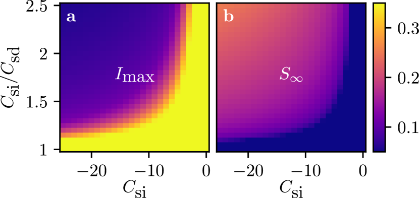
Figure 1: Phase diagram for the SIR-DDFT model. The plots show the dependence of (a) the maximal number of infected persons $I_{\mathrm{max}}$ and (b) the final number of susceptible persons $S_{\infty}$ on the strength of self-isolation $C_{\mathrm{si}}$ and social distancing $C_{\mathrm{sd}}$. A phase boundary is clearly visible.

Measures implemented against a pandemic will typically have two aims: reduction of the total number of infected persons, i.e., making sure that the final number of noninfected persons $S_{\infty}=\lim_{t\to\infty}S(t)$ is large, and reduction of the maximum number of infected persons $I_{\mathrm{max}}$ for keeping the spread within the capacities of the healthcare system. Using parameter scans, we can test whether social distancing and self-isolation can achieve those effects.

As can be seen from the phase diagrams for the SIR-DDFT model shown in Fig. 1, there is a clear phase boundary between the upper left corner, where low values of $I_{\mathrm{max}}$ and high values of $S_{\infty}$ show that the spread of the disease has been significantly reduced, and the rest of the phase diagram, where the disease spreads in essentially the same way as in the model without social distancing. Since all simulations were performed with parameters of $c$ and $w$ that correspond to a disease outbreak in the usual SIR model, this shows that a reduction of social interactions can significantly inhibit epidemic spreading, and that the SIR-DDFT model is capable of demonstrating these effects. The phase boundary shows that, for a reduction of spreading by social measures, two conditions have to be satisfied. First, $|C_{\mathrm{si}}|$ has to be sufficiently large. Second, $|C_{\mathrm{si}}|$ has to be, by a certain amount, larger than $|C_{\mathrm{sd}}|$. Within our physical model of repulsively interacting particles, this arises from the fact that if healthy “particles” are repelled more strongly by other healthy particles than by infected ones, they will spend more time near infected particles and thus are more likely to be infected themselves. Physically, $|C_{\mathrm{si}}|>|C_{\mathrm{sd}}|$ is thus a very reasonable condition given that infected persons, at least once they develop symptoms, will be isolated more strongly than healthy persons.

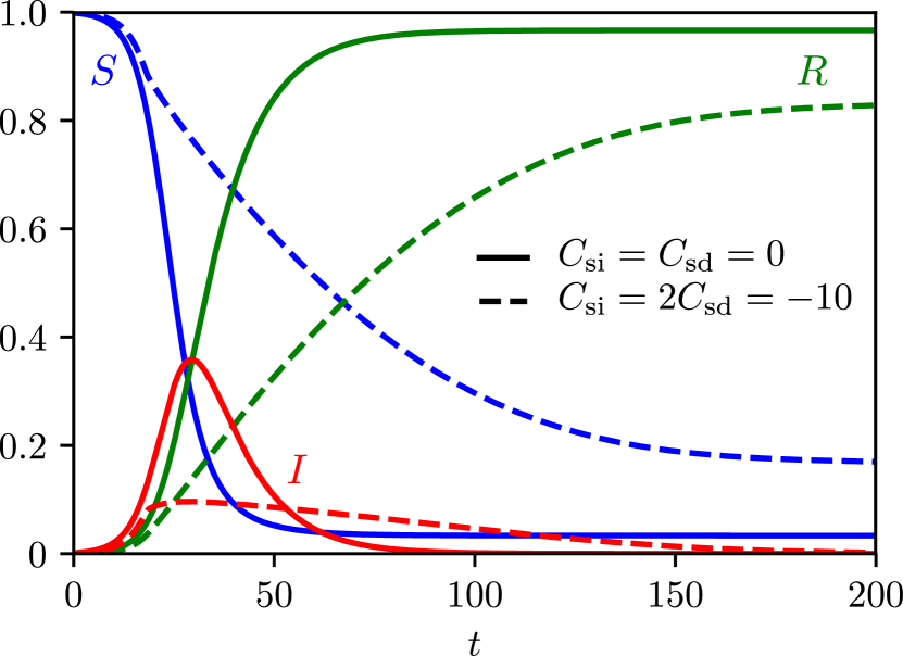
Figure 2: Time evolution of the total number of susceptible, infected, and recovered persons. The time evolution is shown for no interactions ($C_{\mathrm{si}}=C_{\mathrm{sd}}=0$) and for interactions with $C_{\mathrm{si}}=2C_{\mathrm{sd}}=-10$. It can be seen that a reduction of social contacts flattens the curve $I(t)$.

Figure 2 shows the time evolution of the total numbers $S(t)$, $I(t)$, and $R(t)$ of susceptible, infected, and recovered persons, respectively, for the cases without interactions (usual SIR model with diffusion) and with interactions (our model). If no interactions are present (i.e., $C_{\mathrm{si}}=C_{\mathrm{sd}}=0$), $I(t)$ reaches a maximum value of about 0.4 and the pandemic is over at time $t\approx 100$. In the case with interactions (we choose $C_{\mathrm{si}}=2C_{\mathrm{sd}}=-10$, i.e., parameter values inside the social isolation phase), the maximum is significantly reduced to a value of about 0.1. The final value of $R(t)$, which measures the total number of persons that have been infected during the pandemic, decreases from about 1.0 to about 0.8. Moreover, it takes significantly longer (until time $t\approx 200$) for the pandemic to end. This demonstrates that social distancing and self-isolation have the effects they are supposed to have, i.e., to flatten the curve $I(t)$ in such a way that the healthcare system is able to take care of all cases. Notably, all curves were obtained with the same values of $c$ and $w$, i.e., the properties of the disease are identical. Hence, the observed effect is solely a consequence of social interactions. In the usual SIR model, in contrast, these would be accounted for by modifying $c$, such that they could not be studied separately. The theoretical predictions for the effects of quarantine on the course of $I(t)$ (sharp rise, followed by a bend and a flat curve) are in good qualitative agreement with recent data from China John Hopkins University ; Ellyat et al. , where strict regulations were implemented to control the COVID-19 spread Lau et al. (2020).

II.4 Phase separation

To explain the observed phenomena, it is helpful to analyze the spatial distribution of susceptible and infected persons during the pandemic. Figure 3 visualizes $I(x,t)$ with $x=(\vec{r})_{1}$. Interestingly, during the time interval where the pandemic is present, a phase separation can be observed in which the infected persons accumulate at certain spots separated from the susceptible persons. (As this effect is reminiscent of measures that used to be implemented against the spread of leprosy, we refer to these spots as “leper colonies”.) This phase separation is a consequence of the interactions. Since the formation of leper colonies reduces the spatial overlap of the functions $I(x,t)$ and $S(x,t)$, i.e., the amount of contacts between infected and susceptible persons, the total number of infections decreases significantly and it takes longer until enough persons are immune to stop the pandemic.

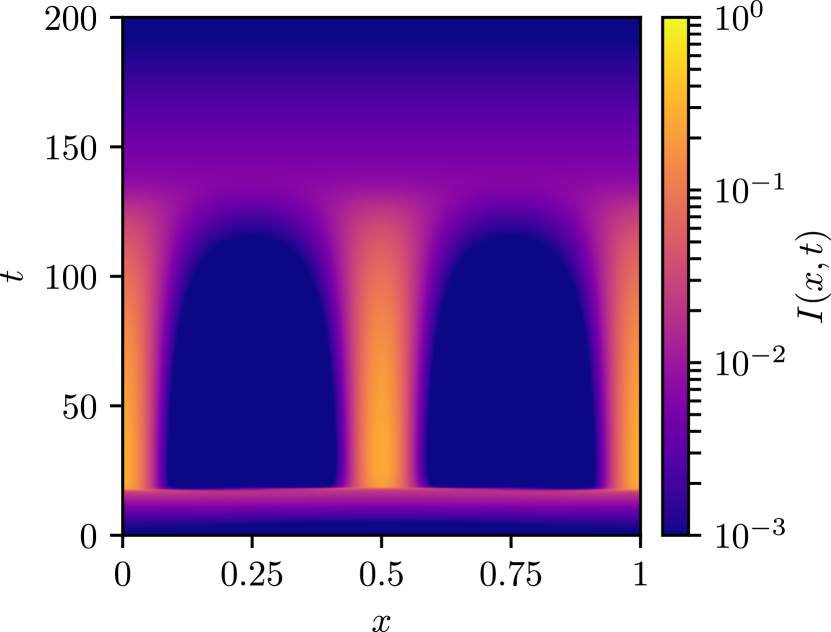
Figure 3: Number of infected persons $\boldsymbol{I(x,t)}$ as a function of space $\boldsymbol{x}$ and time $\boldsymbol{t}$. During the epidemic spreading, the infected persons self-organize into “leper colonies”.

The leper colony transition is an interesting type of nonequilibrium phase behavior in its own right. Recall that we have motivated the SIR-DDFT model based on theories for nonideal chemical reactions. It is thus very likely that effects similar to the ones observed here can be found in chemistry. In this case, they would imply that particle interactions can significantly affect the amount of a certain substance that is produced within a chemical reaction, and that such reactions are accompanied by new types of (transient) pattern formation.

III Discussion

In summary, we have presented a DDFT-based extension of the usual models for epidemic spreading that allows to incorporate social interactions, in particular in the form of self-isolation and social distancing. This has allowed us to analyze the effect of these measures on the spatio-temporal evolution of pandemics. Given the importance of the reduction of social interactions for the control of pandemics, the model provides a highly useful new tool for predicting epidemics and deciding how to react to them. Moreover, it shows an interesting phase behavior relevant for future work on DDFT and nonideal chemical reactions. A possible extension of our model is the incorporation of fractional derivatives Khan and Abdon (2019); Qureshi and Yusuf (2019). Furthermore, enhanced simulations in two spatial dimensions could show interesting pattern formation effects associated with leper colony formation.

IV Methods

IV.1 Linear stability analysis

Here, we perform a linear stability analysis of the extended model given by Eqs. 7, 8 and 9. For the excess free energy, we use the combined Ramakrishnan-Yussouff-Debye-Hückel approximation as in Eqs. 12, 13 and 14, but now with general two-body potentials $U_{\mathrm{sd}}h_{d}(x-x^{\prime})$ for social distancing and $U_{\mathrm{si}}h_{i}(x-x^{\prime})$ for self-isolation. In one spatial dimension, we obtain

$$\begin{split}\partial_{t}S(x,t)&=D_{S}\partial^{2}_{x}S(x,t)-cS(x,t)I(x,t)\\ &\quad-\Gamma_{S}U_{\mathrm{sd}}\partial_{x}\bigg{(}S(x,t)\partial_{x}{\int\;\;\;\mathrm{d}x^{\prime}}\,h_{d}(x-x^{\prime})\\ &\qquad\qquad\qquad\quad(S(x^{\prime},t)+R(x^{\prime},t))\bigg{)}\\ &\quad-\Gamma_{S}U_{\mathrm{si}}\partial_{x}\bigg{(}S(x,t)\partial_{x}{\int\;\;\;\mathrm{d}x^{\prime}}\,h_{i}(x-x^{\prime})I(x^{\prime},t)\bigg{)},\end{split}$$ (17)

$$\begin{split}\partial_{t}I(x,t)&=D_{I}\partial^{2}_{x}I(x,t)+cS(x,t)I(x,t)-wI(x,t)\\ &\quad-\Gamma_{I}U_{\mathrm{si}}\partial_{x}\bigg{(}I(x,t)\partial_{x}{\int\;\;\;\mathrm{d}x^{\prime}}\,h_{i}(x-x^{\prime})\\ &\qquad\qquad\qquad\quad(S(x^{\prime},t)+I(x^{\prime},t)+R(x^{\prime},t))\bigg{)},\end{split}$$ (18)

$$\begin{split}\partial_{t}R(x,t)&=D_{R}\partial^{2}_{x}R(x,t)+wI(x,t)\\ &\quad-\Gamma_{R}U_{\mathrm{sd}}\partial_{x}\bigg{(}R(x,t)\partial_{x}{\int\;\;\;\mathrm{d}x^{\prime}}\,h_{d}(x-x^{\prime})\\ &\qquad\qquad\qquad\quad(S(x^{\prime},t)+R(x^{\prime},t))\bigg{)}\\ &\quad-\Gamma_{R}U_{\mathrm{si}}\partial_{x}\bigg{(}R(x,t)\partial_{x}{\int\;\;\;\mathrm{d}x^{\prime}}\,h_{i}(x-x^{\prime})I(x^{\prime},t)\bigg{)}.\end{split}$$ (19)

Any homogeneous state with $S=S_{0}$, $R=R_{0}$, and $I=0$, where $S_{0}$ and $R_{0}$ are constants, will be a fixed point. We consider fields $S=S_{0}+\tilde{S}$ and $R=R_{0}+\tilde{R}$ with small perturbations $\tilde{S}$ and $\tilde{R}$ and linearize in the perturbations. This results in

$$\begin{split}\partial_{t}\tilde{S}(x,t)&=D_{S}\partial^{2}_{x}\tilde{S}(x,t)-cS_{0}I(x,t)\\ &\quad-S_{0}\Gamma_{S}U_{\mathrm{sd}}\partial^{2}_{x}{\int\;\;\;\mathrm{d}x^{\prime}}\,h_{d}(x-x^{\prime})(\tilde{S}(x^{\prime},t)+\tilde{R}(x^{\prime},t))\\ &\quad-S_{0}\Gamma_{S}U_{\mathrm{si}}\partial^{2}_{x}{\int\;\;\;\mathrm{d}x^{\prime}}\,h_{i}(x-x^{\prime})I(x^{\prime},t),\end{split}$$ (20)

$$\begin{split}\partial_{t}I(x,t)&=D_{I}\partial^{2}_{x}I(x,t)+cS_{0}I(x,t)-wI(x,t),\end{split}$$ (21)

$$\begin{split}\partial_{t}\tilde{R}(x,t)&=D_{R}\partial^{2}_{x}\tilde{R}(x,t)+wI(x,t)\\ &\quad-R_{0}\Gamma_{R}U_{\mathrm{sd}}\partial^{2}_{x}{\int\;\;\;\mathrm{d}x^{\prime}}\,h_{d}(x-x^{\prime})(\tilde{S}(x^{\prime},t)+\tilde{R}(x^{\prime},t))\\ &\quad-R_{0}\Gamma_{R}U_{\mathrm{si}}\partial^{2}_{x}{\int\;\;\;\mathrm{d}x^{\prime}}\,h_{i}(x-x^{\prime})I(x^{\prime},t).\end{split}$$ (22)

We now drop the tilde and make the ansatz $S=S_{1}\exp(\lambda t-\mathrm{i}kx)$, $I=I_{1}\exp(\lambda t-\mathrm{i}kx)$, and $R=R_{1}\exp(\lambda t-\mathrm{i}kx)$. This gives the eigenvalue equation

$$\lambda\begin{pmatrix}S_{1}\\ I_{1}\\ R_{1}\\ \end{pmatrix}=\begin{pmatrix}-D_{S}k^{2}+S_{0}\Gamma_{S}U_{\mathrm{sd}}\hat{h}_{d}(k)k^{2}&S_{0}\Gamma_{S}U_{\mathrm{si}}\hat{h}_{i}(k)k^{2}-cS_{0}&S_{0}\Gamma_{S}U_{\mathrm{sd}}\hat{h}_{d}(k)k^{2}\\ 0&-D_{I}k^{2}+cS_{0}-w&0\\ R_{0}\Gamma_{R}U_{\mathrm{sd}}\hat{h}_{d}(k)k^{2}&w+R_{0}\Gamma_{R}U_{\mathrm{si}}\hat{h}_{i}(k)k^{2}&-D_{R}k^{2}+R_{0}\Gamma_{R}U_{\mathrm{sd}}\hat{h}_{d}(k)k^{2}\end{pmatrix}\!\!\begin{pmatrix}S_{1}\\ I_{1}\\ R_{1}\\ \end{pmatrix}.$$ (23)

Here, $\hat{h}_{d}(k)$ and $\hat{h}_{i}(k)$ are the Fourier transforms of $h_{d}(x-x^{\prime})$ and $h_{i}(x-x^{\prime})$, respectively. The corresponding characteristic polynomial reads

$$\begin{split}(-\lambda-D_{I}k^{2}+cS_{0}-w)&\\ ((-D_{S}k^{2}+S_{0}\Gamma_{S}U_{\mathrm{sd}}\hat{h}_{d}(k)k^{2}-\lambda))&\\ (-D_{R}k^{2}+R_{0}\Gamma_{R}U_{\mathrm{sd}}\hat{h}_{d}(k)k^{2}-\lambda))&\\ -S_{0}R_{0}k^{4}U_{\mathrm{sd}}^{2}\hat{h}_{d}^{2}(k)\Gamma_{S}\Gamma_{R})&=0.\end{split}$$ (24)

Rather than solving this third-order polynomial in $\lambda$ exactly, we consider the limit of long wavelengths. For $k=0$, which corresponds to the usual SIR model given by Eqs. (1)-(3) in the main text if we assume $k^{2}\hat{h}_{d}(k)=0$, Eq. 24 simplifies to

$$(-\lambda+cS_{0}-w)\lambda^{2}=0,$$ (25)

which has the solutions

$$\lambda_{1} =cS_{0}-w,$$ (26)

$$\lambda_{2} =0.$$ (27)

This means that the epidemic will start growing when $cS_{0}>w$, since in this case there is a positive eigenvalue. When interpreting this result, one should take into account that, since a susceptible person that has been infected cannot become susceptible again, the system will, after a small perturbation, not go back to the same state as before even if $w>cS_{0}$. Actually, we have tested the linear stability of the $S$-$R$ plane in phase space, and the fact that any parameter combination of $S_{0}$ and $R_{0}$ with $I=0$ is a solution of the SIR model is reflected by the existence of the eigenvalue $\lambda=0$ with algebraic multiplicity 2 (a perturbation within the $S$-$R$ plane will obviously not lead to an outbreak).

Next, we consider the case $k\neq 0$, but assume that we can neglect the term $S_{0}R_{0}k^{4}U_{\mathrm{sd}}^{2}\hat{h}_{d}^{2}(k)\Gamma_{S}\Gamma_{R}$ in Eq. 24. This corresponds to assuming either $R_{0}=0$ (i.e., we consider the begin of an outbreak of a new disease that no one is yet immune against) or small $k$ (such that terms of order $k^{4}$ can be neglected). Then, Eq. 24 gives

$$\begin{split}(-\lambda-D_{I}k^{2}+cS_{0}-w)&\\ (-D_{S}k^{2}+S_{0}\Gamma_{S}U_{\mathrm{sd}}\hat{h}_{d}(k)k^{2}-\lambda)&\\ (-D_{R}k^{2}+R_{0}\Gamma_{R}U_{\mathrm{sd}}\hat{h}_{d}(k)k^{2}-\lambda)&=0.\end{split}$$ (28)

We can immediately read off the solutions

$$\lambda_{1} =cS_{0}-w-D_{I}k^{2},$$ (29)

$$\lambda_{2} =-D_{S}k^{2}+S_{0}\Gamma_{S}U_{\mathrm{sd}}\hat{h}_{d}(k)k^{2},$$ (30)

$$\lambda_{3} =-D_{R}k^{2}+R_{0}\Gamma_{R}U_{\mathrm{sd}}\hat{h}_{d}(k)k^{2}.$$ (31)

The result for $\lambda_{1}$ shows that the initial state still becomes unstable for $cS_{0}>w$, i.e., the interactions cannot stabilize a state without infected persons that would be unstable otherwise. The eigenvalues $\lambda_{2}$ and $\lambda_{3}$, which were 0 in the long-wavelength limit, now describe the dispersion due to interparticle interactions that may lead to instabilities not related to disease outbreak.

IV.2 Front speed

For determining the propagation speed of fronts, we can use the marginal stability hypothesis Dee and Langer (1983); Ben-Jacob et al. (1985); Archer et al. (2012, 2014, 2016). We transform to the co-moving frame that has velocity $v$ and assume that the growth rate in this frame is zero at the leading edge. Thereby, we obtain for a general dispersion $\lambda(k)$ the equations

$$\mathrm{i}v+\frac{\mathrm{d}\lambda}{\mathrm{d}k} =0,$$ (32)

$$\operatorname{Re}(\mathrm{i}vk+\lambda) =0.$$ (33)

These equations can be solved for the complex wavenumber $k=k_{\mathrm{re}}+\mathrm{i}k_{\mathrm{im}}$ and the velocity $v$. For the dispersion $\lambda_{1}=cS_{0}-w-D_{I}k^{2}$ (we are interested in instabilities associated with infections), Eqs. 32 and 33 lead to

$$\mathrm{i}v-2\mathrm{i}D_{I}k_{\mathrm{im}} =0,$$ (34)

$$-2D_{I}k_{\mathrm{re}} =0,$$ (35)

$$-vk_{\mathrm{im}}+cS_{0}-w-D_{I}(k_{\mathrm{re}}^{2}-k_{\mathrm{im}}^{2}) =0.$$ (36)

The solution of these equations is

$$k_{\mathrm{re}} =0,$$ (37)

$$k_{\mathrm{im}} =\pm\sqrt{\frac{cS_{0}-w}{D_{I}}},$$ (38)

$$v =2\sqrt{D_{I}(cS_{0}-w)},$$ (39)

which is in agreement with results from the literature Naether et al. (2008). Front speeds for dispersions of the form (30) and (31) can be found in Ref. Archer et al. (2012).

IV.3 Numerical analysis

The calculation was done in one spatial dimension on the domain $x\in[0,1]$ with periodic boundary conditions, using an explicit finite-difference scheme with step size $\mathrm{d}x=0.005$ (individual simulations) or $\mathrm{d}x=0.01$ (parameter scan) and adaptive time steps. As an initial condition, we use a Gaussian peak with amplitude $1$ and variance $50^{-2}$ centered at $x=0.5$ for $S(x,0)$, $I(x,0)=0.001S(x,0)$, and $R(x,0)=0$. Since the effect of the parameters $c$ and $w$ on the dynamics is known from previous studies of the SIR model, we fix their values to $c=1$ and $w=0.1$ to allow for an outbreak. Moreover, we set $\Gamma_{S}=\Gamma_{I}=\Gamma_{R}=1$, $D_{S}=D_{I}=D_{R}=0.01$, and $\sigma_{\mathrm{sd}}=\sigma_{\mathrm{si}}=100$.

References

- Poland and Dennis (1998) J. D. Poland and D. T. Dennis, “Plague,” in Bacterial Infections of Humans (Springer, Boston, 1998) pp. 545–558.
- Wilton (1993) P. Wilton, “Spanish flu outdid WWI in number of lives claimed,” Canadian Medical Association Journal 148, 2036–2037 (1993).
- Cliff and Smallman-Raynor (2013) A. Cliff and M. Smallman-Raynor, Oxford textbook of infectious disease control: a geographical analysis from medieval quarantine to global eradication (Oxford University Press, Oxford, 2013).
- Wu et al. (2020) F. Wu, S. Zhao, B. Yu, Y.-M. Chen, W. Wang, Z.-G. Song, Y. Hu, Z.-W. Tao, J.-H. Tian, Y.-Y. Pei, et al., “A new coronavirus associated with human respiratory disease in China,” Nature 579, 265–269 (2020).
- Zhou et al. (2020) P. Zhou, X.-L. Yang, X.-G. Wang, B. Hu, L. Zhang, W. Zhang, H.-R. Si, Y. Zhu, B. Li, C.-L. Huang, et al., “A pneumonia outbreak associated with a new coronavirus of probable bat origin,” Nature 579, 270–273 (2020).
- Cui et al. (2019) J. Cui, F. Li, and Z.-L. Shi, “Origin and evolution of pathogenic coronaviruses,” Nature Reviews Microbiology 17, 181–192 (2019).
- Wang et al. (2020) C. Wang, P. W. Horby, F. G. Hayden, and G. F. Gao, “A novel coronavirus outbreak of global health concern,” Lancet 395, 470–473 (2020).
- Li et al. (2020) R. Li, S. Pei, B. Chen, Y. Song, T. Zhang, W. Yang, and J. Shaman, “Substantial undocumented infection facilitates the rapid dissemination of novel coronavirus (SARS-CoV2),” Science, in press, eabb3221 (2020).
- Stein (2020) R. Stein, “COVID-19 and rationally layered social distancing,” International Journal of Clinical Practice, in press, e13501 (2020).
- Ferguson et al. (2020) N. M. Ferguson, D. Laydon, G. Nedjati-Gilani, N. Imai, K. Ainslie, M. Baguelin, S. Bhatia, A. Boonyasiri, Z. Cucunubá, G. Cuomo-Dannenburg, et al., “Impact of non-pharmaceutical interventions (NPIs) to reduce COVID-19 mortality and healthcare demand,” London: Imperial College COVID-19 Response Team, March 16 (2020).
- Mizumoto and Chowell (2020) K. Mizumoto and G. Chowell, “Transmission potential of the novel coronavirus (COVID-19) onboard the Diamond Princess cruises ship, 2020,” Infectious Disease Modelling 5, 264–270 (2020).
- Lau et al. (2020) H. Lau, V. Khosrawipour, P. Kocbach, A. Mikolajczyk, J. Schubert, J. Bania, and T. Khosrawipour, “The positive impact of lockdown in Wuhan on containing the COVID-19 outbreak in China,” Journal of Travel Medicine, in press, taaa037 (2020), 10.1093/jtm/taaa037.
- Marini Bettolo Marconi and Tarazona (1999) U. Marini Bettolo Marconi and P. Tarazona, “Dynamic density functional theory of fluids,” Journal of Chemical Physics 110, 8032–8044 (1999).
- Archer and Evans (2004) A. J. Archer and R. Evans, “Dynamical density functional theory and its application to spinodal decomposition,” Journal of Chemical Physics 121, 4246–4254 (2004).
- Cai et al. (2015) W. Cai, L. Chen, F. Ghanbarnejad, and P. Grassberger, “Avalanche outbreaks emerging in cooperative contagions,” Nature Physics 11, 936–940 (2015).
- Leventhal et al. (2015) G. E. Leventhal, A. L. Hill, M. A. Nowak, and S. Bonhoeffer, “Evolution and emergence of infectious diseases in theoretical and real-world networks,” Nature Communications 6, 6101 (2015).
- De Domenico et al. (2016) M. De Domenico, C. Granell, M. A. Porter, and A. Arenas, “The physics of spreading processes in multilayer networks,” Nature Physics 12, 901–906 (2016).
- Gómez-Gardenes et al. (2018) J. Gómez-Gardenes, D. Soriano-Panos, and A. Arenas, “Critical regimes driven by recurrent mobility patterns of reaction-diffusion processes in networks,” Nature Physics 14, 391–395 (2018).
- Kermack and McKendrick (1927) W. O. Kermack and A. G. McKendrick, “A contribution to the mathematical theory of epidemics,” Proceedings of the Royal Society of London. Series A, Containing papers of a Mathematical and Physical Character 115, 700–721 (1927).
- Nesteruk (2020) I. Nesteruk, “Statistics based predictions of coronavirus 2019-nCoV spreading in mainland China,” preprint, medRxiv (2020), 10.1101/2020.02.12.20021931.
- Simha et al. (2020) A. Simha, R. V. Prasad, and S. Narayana, “A simple stochastic SIR model for COVID-19 infection dynamics for Karnataka: learning from Europe,” preprint, arXiv:2003.11920 (2020).
- Zhong et al. (2020) P. Zhong, S. Guo, and T. Chen, “Correlation between travellers departing from Wuhan before the spring festival and subsequent spread of COVID-19 to all provinces in China,” Journal of Travel Medicine, in press, taaa036 (2020), 10.1093/jtm/taaa036.
- Wang and Wu (2018) L. Wang and J. T. Wu, “Characterizing the dynamics underlying global spread of epidemics,” Nature Communications 9, 1–11 (2018).
- Colizza et al. (2007) V. Colizza, R. Pastor-Satorras, and A. Vespignani, “Reaction-diffusion processes and metapopulation models in heterogeneous networks,” Nature Physics 3, 276–282 (2007).
- Postnikov and Sokolov (2007) E. B. Postnikov and I. M. Sokolov, “Continuum description of a contact infection spread in a SIR model,” Mathematical Biosciences 208, 205–215 (2007).
- Naether et al. (2008) U. Naether, E. B. Postnikov, and I. M. Sokolov, “Infection fronts in contact disease spread,” European Physical Journal B 65, 353–359 (2008).
- Belik et al. (2011) V. Belik, T. Geisel, and D. Brockmann, “Natural human mobility patterns and spatial spread of infectious diseases,” Physical Review X 1, 011001 (2011).
- Wang et al. (2012) W. Wang, Y. Cai, M. Wu, K. Wang, and Z. Li, “Complex dynamics of a reaction-diffusion epidemic model,” Nonlinear Analysis: Real World Applications 13, 2240–2258 (2012).
- Bacaër and Sokhna (2005) N. Bacaër and C. Sokhna, “A reaction-diffusion system modeling the spread of resistance to an antimalarial drug,” Mathematical Biosciences & Engineering 2, 227–238 (2005).
- Peng and Liu (2009) R. Peng and S. Liu, “Global stability of the steady states of an SIS epidemic reaction-diffusion model,” Nonlinear Analysis: Theory, Methods & Applications 71, 239–247 (2009).
- Archer and Rauscher (2004) A. J. Archer and M. Rauscher, “Dynamical density functional theory for interacting Brownian particles: stochastic or deterministic?” Journal of Physics A: Mathematical and General 37, 9325–9333 (2004).
- Archer (2005) A. J. Archer, “Dynamical density functional theory: binary phase-separating colloidal fluid in a cavity,” Journal of Physics: Condensed Matter 17, 1405–1427 (2005).
- Wittkowski et al. (2012) R. Wittkowski, H. Löwen, and H. R. Brand, “Extended dynamical density functional theory for colloidal mixtures with temperature gradients,” Journal of Chemical Physics 137, 224904 (2012).
- Español and Löwen (2009) P. Español and H. Löwen, “Derivation of dynamical density functional theory using the projection operator technique,” Journal of Chemical Physics 131, 244101 (2009).
- te Vrugt and Wittkowski (2019a) M. te Vrugt and R. Wittkowski, “Projection operators in statistical mechanics: a pedagogical approach,” preprint, arXiv:2001.01572 (2019a).
- Lutsko (2016) J. F. Lutsko, “Mechanism for the stabilization of protein clusters above the solubility curve: the role of non-ideal chemical reactions,” Journal of Physics: Condensed Matter 28, 244020 (2016).
- Lutsko and Nicolis (2016) J. F. Lutsko and G. Nicolis, “Mechanism for the stabilization of protein clusters above the solubility curve,” Soft Matter 12, 93–98 (2016).
- Liu and Liu (2020) Y. Liu and H. Liu, “Development of reaction-diffusion DFT and its application to catalytic oxidation of NO in porous materials,” AIChE Journal 66, e16824 (2020).
- Méndez-Valderrama et al. (2018) J. F. Méndez-Valderrama, Y. A. Kinkhabwala, J. Silver, I. Cohen, and T. A. Arias, “Density-functional fluctuation theory of crowds,” Nature Chemistry 9, 3538 (2018).
- Al-Saedi et al. (2018) H. M. Al-Saedi, A. J. Archer, and J. Ward, “Dynamical density-functional-theory-based modeling of tissue dynamics: application to tumor growth,” Physical Review E 98, 022407 (2018).
- Angioletti-Uberti et al. (2018) S. Angioletti-Uberti, M. Ballauff, and J. Dzubiella, “Competitive adsorption of multiple proteins to nanoparticles: the Vroman effect revisited,” Molecular Physics 116, 3154–3163 (2018).
- Martínez-García et al. (2013) R. Martínez-García, J. M. Calabrese, T. Mueller, K. A. Olson, and C. López, “Optimizing the search for resources by sharing information: Mongolian gazelles as a case study,” Physical Review Letters 110, 248106 (2013).
- Wensink and Löwen (2008) H. H. Wensink and H. Löwen, “Aggregation of self-propelled colloidal rods near confining walls,” Physical Review E 78, 031409 (2008).
- Wittkowski and Löwen (2011) R. Wittkowski and H. Löwen, “Dynamical density functional theory for colloidal particles with arbitrary shape,” Molecular Physics 109, 2935–2943 (2011).
- Menzel et al. (2016) A. M. Menzel, A. Saha, C. Hoell, and H. Löwen, “Dynamical density functional theory for microswimmers,” Journal of Chemical Physics 144, 024115 (2016).
- Hoell et al. (2019) C. Hoell, H. Löwen, and A. M. Menzel, “Multi-species dynamical density functional theory for microswimmers: derivation, orientational ordering, trapping potentials, and shear cells,” Journal of Chemical Physics 151, 064902 (2019).
- Pototsky and Stark (2012) A. Pototsky and H. Stark, “Active Brownian particles in two-dimensional traps,” Europhysics Letters 98, 50004 (2012).
- Wittmann and Brader (2016) R. Wittmann and J. M. Brader, “Active Brownian particles at interfaces: an effective equilibrium approach,” Europhysics Letters 114, 68004 (2016).
- Wittmann et al. (2017) R. Wittmann, U. Marini Bettolo Marconi, C. Maggi, and J. M. Brader, “Effective equilibrium states in the colored-noise model for active matter II. A unified framework for phase equilibria, structure and mechanical properties,” Journal of Statistical Mechanics: Theory and Experiment 2017, 113208 (2017).
- te Vrugt (2020) M. te Vrugt, “The five problems of irreversibility,” in preparation (2020).
- Schindler et al. (2019) T. Schindler, R. Wittmann, and J. M. Brader, “Particle-conserving dynamics on the single-particle level,” Physical Review E 99, 012605 (2019).
- Mori (1965) H. Mori, “Transport, collective motion, and Brownian motion,” Progress of Theoretical Physics 33, 423–455 (1965).
- Zwanzig (1960) R. Zwanzig, “Ensemble method in the theory of irreversibility,” Journal of Chemical Physics 33, 1338–1341 (1960).
- te Vrugt and Wittkowski (2019b) M. te Vrugt and R. Wittkowski, “Mori-Zwanzig projection operator formalism for far-from-equilibrium systems with time-dependent Hamiltonians,” Physical Review E 99, 062118 (2019b).
- Zhu et al. (2019) P. Zhu, X. Wang, S. Li, Y. Guo, and Z. Wang, “Investigation of epidemic spreading process on multiplex networks by incorporating fatal properties,” Applied Mathematics and Computation 359, 512–524 (2019).
- Berge et al. (2017) T. Berge, J. M.-S. Lubuma, G. M. Moremedi, N. Morris, and R. Kondera-Shava, “A simple mathematical model for Ebola in Africa,” Journal of Biological Dynamics 11, 42–74 (2017).
- Zhu (2020) W. Zhu, “Should, and how can, exercise be done during a coronavirus outbreak? An interview with Dr. Jeffrey A. Woods,” Journal of Sport and Health Science 9, 105–107 (2020).
- Malijevskỳ and Archer (2013) A. Malijevskỳ and A. J. Archer, “Sedimentation of a two-dimensional colloidal mixture exhibiting liquid-liquid and gas-liquid phase separation: a dynamical density functional theory study,” Journal of Chemical Physics 139, 144901 (2013).
- Ramakrishnan and Yussouff (1979) T. V. Ramakrishnan and M. Yussouff, “First-principles order-parameter theory of freezing,” Physical Review B 19, 2775–2794 (1979).
- Hansen and McDonald (2009) J.-P. Hansen and I. R. McDonald, Theory of Simple Liquids: with Applications to Soft Matter, 4th ed. (Elsevier Academic Press, Oxford, 2009).
- Dee and Langer (1983) G. Dee and J. S. Langer, “Propagating pattern selection,” Physical Review Letters 50, 383–386 (1983).
- Ben-Jacob et al. (1985) E. Ben-Jacob, H. Brand, G. Dee, L. Kramer, and J. S. Langer, “Pattern propagation in nonlinear dissipative systems,” Physica D: Nonlinear Phenomena 14, 348–364 (1985).
- Archer et al. (2012) A. J. Archer, M. J. Robbins, U. Thiele, and E. Knobloch, “Solidification fronts in supercooled liquids: how rapid fronts can lead to disordered glassy solids,” Physical Review E 86, 031603 (2012).
- Archer et al. (2014) A. J. Archer, M. C. Walters, U. Thiele, and E. Knobloch, “Solidification in soft-core fluids: disordered solids from fast solidification fronts,” Physical Review E 90, 042404 (2014).
- Archer et al. (2016) A. J. Archer, M. C. Walters, U. Thiele, and E. Knobloch, “Generation of defects and disorder from deeply quenching a liquid to form a solid,” in Mathematical Challenges in a New Phase of Materials Science (Springer, Kyoto, 2016) pp. 1–26.
- (66) John Hopkins University, “Coronavirus COVID-19 Global Cases by the Center for Systems Science and Engineering at John Hopkins University,” \seqsplithttps://gisanddata.maps.arcgis.com/apps/opsdashboard/index.html#/bda7594740fd40299423467b48e9ecf6, visited 2020-03-29.
- (67) H. Ellyat, W. Tan, and Y. N. Lee, “UK warns fifth of workforce could be off sick from coronavirus at its peak; army prepared,” \seqsplithttps://www.cnbc.com/2020/03/03/coronavirus-live-updates-china-reports-125-new-cases-as-its-numbers-drop.html, visited 2020-03-29.
- Khan and Abdon (2019) M. A. Khan and A. Abdon, “Dynamics of Ebola disease in the framework of different fractional derivatives,” Entropy 21, 303 (2019).
- Qureshi and Yusuf (2019) S. Qureshi and A. Yusuf, “Fractional derivatives applied to MSEIR problems: comparative study with real world data,” European Physical Journal Plus 134, 171 (2019).