Role of disorder and fluctuation on charge migration dynamics in molecular aggregate with quantum mechanical network

Abstract

We examine the effect of structural disorder and dynamical lattice fluctuation on charge migration dynamics starting from a birth of local exciton in a quantum network of molecular aggregates by using model Hamiltonians having complicate interactions. Here all monomers are supposed to be the same for simplicity. A natural use of inherent sparsity of Hamiltonian matrix allows us an investigation of essential features in quantum network dynamics accompanied with a fluctuation of interaction. Variation of disorder parameter, kinetic energy and effective mass of monomers in electron dynamics calculation reveal how static disorder and dynamical fluctuation affects electron dynamics in a large size of molecular aggregates. Disorder in aggregate structure suppress charge separation while molecular motion can promote charge diffusion in cases of smaller mass. These findings are obtained by using a newly introduced formula for evaluating charge separation in molecular aggregates that is useful for other analysis involved with charge migration dynamics in molecular/atom aggregates. This work provides a way for obtaining a quantum mechanical time-dependent picture of diffusion and migration of exciton and charge density in general molecular aggregates, which offers a fundamental understanding of electronic functionality of nanocomposites.

I Introduction

Exciton and following charge migration is important and ubiquitous in photo energy conversion process in material. A photo excited exciton is a source of charge separation leading to chemical driving force. Sundstrom-review-solar-energy ; accum-CS Fundamentally and microscopically, they are described by quantum dynamics. Though a picture of charge separation is still unrevealed, experimental observations of time dependent charge separation and their control have been reported in pico second and nano second time scales. Nakajima-JPCL2012-CS-obs-ps ; image-CS-CR In order to understand charge separation mechanism we need a time dependent picture fine enough to include chemical reaction within sub-pico-second.

Because a fully ab initio description of charge separation in quantum dynamics theory is computationally tough, an investigation of interesting features related to a realistic size of molecular aggregate system accompanied with fluctuation have been limited. To overcome this, we utilize a simplified tight-binding model having sparsity in a molecular aggregate Hamiltonian matrix, referential occupation of quantum sub-states inside monomers and Liouville–von Neumman equation. We can reduce a computational cost using this sparsity of interaction network in molecular aggregates associated fast spatial damping of electron coupling expected in realistic material system.

Based on this, we demonstrate an efficient scheme for examining a time dependent behavior of charge separation. We investigate how static and dynamical disorder affect a charge separation after a birth of exciton in molecular aggregate system. Here, static and dynamical disorders mean initial disorder in reference structure and time-dependent deformation of configuration of aggregate, respectively.

Here we examine a quantum dynamics of excited electrons without resorting to method using too much coarse graining treatment such as kinetic Monte Carlo schemes because they can never tell about a microscopic origin inherent in this kind of phenomena, for example, quantum mechanical interference, decoherence and dynamical resonance, and so on. These methods are complementary. In fact, the latter Monte Carlo type kinematic methods have been successfully used for the description in a wide range from middle to macroscopic scale. Madigan-PRL2006 ; Sousa-JCP2018

We here focus on a shorter time scale and smaller systems compared to such a macroscopic view, namely, middle scale description with respect to time and spatial size. By introducing and using a new concise scheme, we intend to propose an origin of excitation driven charge migration in a moderate size of molecular aggregate systems.

In the next section, II, theoretical method is explained by focusing a Hamiltonian sparsity for molecular aggregates. That is followed by the numerical section, III, for demonstrating the present scheme using fused lattice structure system consisting of simplified monomers having local quantum sites. There, we introduce charge diffusion and separation measure and discuss effects of structure fluctuation and static disorder. In Sect. IV we conclude this article with a future perspective about the present scheme.

II Theoretical method

We briefly explain the general formulation of the developed calculation method aimed for a concise description and examination of exciton and charge migration. Generalization with respect to state number and couplings is formally straightforward. The sparsity of Hamiltonian matrix is utilized for attaining a reduction of computational cost.

II.1 Sparse form of Hamiltonian matrix having a network structure in interactions of quantum states

For a compact and economical calculation of quantum dynamics supported by a sparcity in a network associated with Hamiltonian matrix, instead of treating full matrix elements

$$\{H_{\alpha\beta}\}_{\alpha,\beta=1\sim N_{\rm{basis}}},$$ (1)

we employ a following data structure as the expression of this matrix,

$$\{\alpha_{i},\beta_{i},H_{\alpha_{i}\beta_{i}}\}_{i=1\sim N_{\textrm{pair}}}.$$ (2)

Here $N_{\textrm{pair}}$ is a number of non-zero elements in the original matrix. To be more precise practically, for an infinitesimal threshold value $\eta$, $N_{\textrm{pair}}$ is the number of elements in the set $\{H_{\alpha\beta};|H_{\alpha\beta}|\geq\eta\}$. Practically we can establish $\eta$ as a function of a spatial distance of pair subsystems.

Next, we provide a block structure associated with a molecular aggregation that we are interested in here. Total basis number $N_{\textrm{basis}}$ is the same as a sum of numbers of quantum states given for all subsystems, $N_{\textrm{basis}}=\sum_{a=1}^{N_{\textrm{g}}}M_{I}(a)$, with $M_{I}(a)$ being the number of internal quantum states in subsystem $a$. $N_{\textrm{g}}$ is a number of group sites. The total Hamiltonian matrix is divided into $N_{\rm{g}}^{2}$ sectors and the $(a,b)$-th block takes a matrix form having a size of $M_{I}(a)\times M_{I}(b)$ where $a$ and $b$ in $(a,b)$ denote positions of row and column, respectively. $a=b$ and $a\neq b$ correspond respectively to local Hamiltonian of subsystem $a$ and coupling matrix between $a$ and $b$. Practically, the number of multiplication of their elements to other matrix is reduced effectively accompanied with a small additional cost in pointer skip in a memory space. We refer to this as a compressed Hamiltonian matrix (CHM).

As a final part of this subsection, for making clear the sector-ed structure, we define a one-to-one mapping between an index label of original matrix and an index pair in sector-ed matrix as $\{k\Leftrightarrow(a,\alpha_{a})\}$ with $1\leq k\leq N_{\textrm{basis}}$, $1\leq a\leq N_{\textrm{g}}$ and $1\leq\alpha_{a}\leq M_{I}(a)$.

II.2 Liouville–von Neuman equation using multiplication of compressed Hamiltonian matrix

Using CHM, a time derivative of density matrix $\rho_{\alpha\beta}$ in LvN equation,

$$\dfrac{d\rho_{\alpha\beta}}{dt}=-\dfrac{i}{\hbar}\sum_{\gamma}^{Nb}\left\{\rho_{\alpha\gamma}H_{\gamma\beta}-H_{\alpha\gamma}\rho_{\gamma\beta}\right\},$$ (3)

can be cast into the following pseudo code:

$$\omega:=0$$

$$do\quad i=1,\,\,N_{\textrm{pa}}$$

$$\quad do\quad p=1,\,\,N_{b}$$

$$\quad\quad\omega_{p\beta_{i}}:=\omega_{p\beta_{i}}-\dfrac{i}{\hbar}\rho_{p\alpha_{i}}H_{\alpha_{i}\beta_{i}}$$

$$\quad enddo$$

$$\quad do\quad q=1,\,\,N_{b}$$

$$\quad\quad\omega_{\alpha_{i}q}:=\omega_{\alpha_{i}q}-\left(-\dfrac{i}{\hbar}H_{\alpha_{i}\beta_{i}}\rho_{\beta_{i}q}\right)$$

$$\quad enddo$$

$$enddo$$ (4)

with $\omega\equiv\dfrac{d}{dt}\rho$.

II.3 Structure of model Hamiltonian employed here

We briefly summarize a specific form of Hamiltonian employed here for a demonstration of the present method.

Each block bare sub-Hamiltonian sector for subsystem a is $H^{aa;0}_{i_{a}j_{a}}=\delta_{i_{a}j_{a}}\epsilon^{a}_{i_{a}}$. Coupling off-diagonal block sectors for different subsystems, a and b, are given by $H_{i_{a}j_{b}}^{ab}(R_{ab})=s_{i_{a}i_{b}}^{ab}\rm{exp}\left(-R_{ab}/R^{\rm damp}_{i_{a}j_{b}}\right)$. Here, $R_{ab}$ denotes distance between subsystems a and b while $R^{\rm damp}_{i_{a}j_{b}}$ are the parameters that determine a damping strength with respect to $R_{ab}$. Range of indicies are $a,b=1,2,...,N_{\textrm{g}}$ and $i_{a}=1,2,...,M_{I}(a)$. For taking into account an effect of structure dynamics in a simulation, diagonal elements in each block sub-Hamiltonian sector for subsystem $a$ were designed to change as a function of distance of each pair subsystems in a form of $H_{i_{a}i_{a}}^{aa}=H^{aa;0}_{i_{a}i_{a}}+\sum_{b\neq a}\dfrac{1}{4}k^{\textrm{spring}}(R_{ab}-R_{ab}^{\textrm{ref}})^{2}$. In this equation we used 1/4 but not 1/2 for avoiding an apparent double counting so that the spring constant, $k^{\textrm{spring}}$, should keep physical meaning.

II.4 Time propagation

For computational efficiency, we use the Chebyshev expansion method for the time propagation operator associated with LvN equation of motion. The formalism of this time propagation method is summarized in Appendix A for self-containednes, of which theoretical details are given in the work by Guo et al. Guo-JCP1999-Cheby-LvN

The time increment for each time step used in this article was set to 4 a.u., which was sufficient for the conversion of the result, now shown here. The number of time steps in simulation is 500 and total time is 2000 a.u. which is 48.3 fs.

III Numerical demonstration

III.1 Effective Charge distance from reference point

Here we examine how a charge pattern emerges after a birth of local exciton at the center in a generally disordered lattice system consisting of molecular monomers.

This preparation of initial excitation is intended for examining inherent feature of dispersion that a quantum mechanical network has.

For this purpose, we construct an evaluation formula for effective position of wave fronts represented by $u^{+}$ and $u^{-}$ for positive and negative charge roughly measured from position of initial exciton.

• Calculate sum of positive and negative charge over the sites as
  

  $$q_{\textrm{sum}}^{\pm}=\sum_{g}^{\textrm{site}}h(\pm q_{g})\,q_{g}\quad$$ (5)

  $h(x)$ is the Heaviside function and takes 1 and 0 respectively for x $>$ 0 and x $\leq$ 0.

• Evaluate weighted sum of positive negative charge multiplied with the distance from the reference position over the sites as
  

  $$u^{\pm}=\sum_{g}^{\textrm{site}}h(\pm q_{g})\,q_{g}|{\bf r}_{g}-{\bf r}_{\textrm{ref}}|\quad$$ (6)

• Normalize $u^{+}$ and $u^{-}$ by using $q_{\textrm{sum}}^{+}$ and $q_{\textrm{sum}}^{-}$. And then, determine the effective propagation front of positive and negative charge as

  $$d^{\pm}=u^{\pm}/q_{\textrm{sum}}^{\pm}$$ (7)

The charge on each site is evaluated as the difference of quantum population in the corresponding site from the reference occupancy. In the following numerical demonstration, each site has two quantum states of local ground and excited states with $M_{I}=2$ and an reference occupation only in the ground state.

For each initial structure we prepared randomly 30 velocity vectors for the geometries having disorder parameter $f$ being fixed and took average and variations of $d^{\pm}$.

Magnitude of each velocity vector of monomer was determined so as to match with equivalently divided amount of energies according to micro-canonical temperature, 0 and 300 K while the directions of vectors were given randomly.

III.2 Details

First of all in the presentation, we summarize the calculation conditions including system parameters employed here.

For simplicity we set the two internal quantum states for each, namely, we set $M_{I}(a)=2$ with a referential occupancy for lowest one be hypothetical setting of use of HOMO and LUMO for arbitrary monomer $a$ in the system. Below we express $M_{I}(a)=M_{I}$. Since a three dimensional calculation is computationally demanding, we treat two dimensional model that still has a significance as a starting point for investigating electron dynamics in a surface of molecular crystal. The energies of these two states are commonly set to be $\epsilon^{a}_{1}=0.0$ and $\epsilon^{a}_{2}=0.3$ Hartree for all $a$ that appear in each block matrix placed at diagonal position in a whole Hamiltonian matrix. We selected this energy difference $\epsilon^{a}_{2}-\epsilon^{a}_{1}=0.3$ similar to HOMO-LUMO gap of naphthalene obtained by CAM-B3LYP/6-31G(d) calculation at optimized geometry, 0.2731 Hartree. We note that a naphthalene serves as an electron donor molecule, for example, in a naphthalene - tetra-cyano-ethylene dimer. Therefore, the employed test model of molecular aggregate is expected to have a hole transfer property.

As a referential spatial configuration of monomer positions, we employed square lattice on x-y plane of which numbers of rows and columns are expressed by $n_{x}$ and $n_{y}$ with $n_{x}=n_{y}$. The total number of monomers are $N_{\textrm{g}}=n_{x}n_{y}$. In this article, we examine two cases of $n_{x}=n_{y}=25$ and $31$ with fixed reference distance of nearest monomers being $D_{x}=D_{y}=7.8$, respectively. Later we simply express $D_{x}=D_{y}$ as $D$. Note that in dynamics calculations they change according to the introduced disorder of geometrical structure at initial simulation time and time-dependent deformation of configuration, which is followed by a clear illustration of a significant effect on charge migration dynamics after a birth of local excitation. Total number of elements in a basis set are given by $N_{\textrm{basis}}=N_{\textrm{g}}M_{I}$.

We introduced a disorder to initial geometry of locations of monomers in aggregate by giving random displacement $(\eta-0.5)fD$ for them in each Cartesian coordinate, x and y compared from reference positions within a lattice structure. Here $\eta$ being random number over $[0:1]$ while $f$ is a parameter that modulate the degree of disorder, that we call disorder parameter. In this article, we compare the results with variation of $f$ = 0.0, 0.2 and 0.4.

Time increments in dynamics calculation commonly used for quantum and classical degrees of freedoms are commonly set to efficiently and practically small value, 4 au. Total simulation time is $T_{\textrm{max}}=2000$ with a number of time steps $N_{\textrm{t}}$ being 500.

Then, we briefly explain model functions used in construction of Hamiltonian matrix. The elements of damping matrix of monomer interaction matrices $H_{i_{a}i_{b}}^{ab}(R_{ab})$ were set as $R^{\textrm{damp}}_{i_{a}j_{a}}=1.2$ Å ( = 2.268 Bohr ) for all $i_{a},j_{a}=1\sim M_{I}(a)$ and $a$ while strength amplitude matrices in integration matrices were supposed to be $s_{11}^{ab}=0.3$, $s_{12}^{ab}=s_{21}^{ab}=1.5$, and $s_{22}^{ab}=1.0$. A threshold parameter for monomer pairing interaction is set to $r_{\textrm{pair}}$ = 10.8. Monomer interactions in a total Hamiltonian matrix were taken into account only for monomer pairs having distances being less that $r_{\textrm{pair}}$, which characterize sparsity of Hamiltonian for aggregate system. We checked that this value of $r_{\textrm{pair}}$ is sufficiently large for the convergence of results with use of damping matrix $R^{\textrm{damp}}_{i_{a}j_{a}}$ and strength matrix $s_{i_{a}j_{b}}^{ab}$ in monomer interaction mentioned above.

Masses of uniform monomer were varied as $\mu=5\times 10^{4}$, $1\times 10^{5}$ and $2\times 10^{5}$ for examining a kinematic effect on charge migration dynamics. The spring constant of hypothetical harmonic potential for each monomer pair was commonly set to $k^{\textrm{spring}}=0.002$ throughout dynamics calculations. In order to obtain a fundamental information on a propensity of charge migration dynamics, we utilized an introduction of a local exciton as a sudden perturbation in quantum state of whole the system at the initial simulation time. In all the dynamics calculations, central monomer was initially locally excited from the lowest to highest state with a half amount of quantum population, which corresponds to hypothetical HOMO-LUMO excitation.

Each portion of initial kinetic energy in 2$N_{\textrm{g}}$ all the classical degrees of freedom of molecular aggregates confined in x-y plane was set to $\frac{1}{2}k_{\textrm{B}}T$ with the variation of micro-canonical temperature $T$ being 0 and 300 Kelvin. Here $k_{\textrm{B}}$ denotes the Boltzmann constant. Direction of velocity vectors for each monomer was randomly given. In all the simulations, we employed 30 sets of sample initial velocities for taking average of quantum properties. In the present simulation time scale, effect of a bounce of excitons and front of charge wave from peripheral edge of the whole lattice is negligible.

Finally, we briefly show the efficiency of the present method using Eq.(4) based on the sparsity of Hamiltonian of molecular aggregate. Comparisons of computational cost with the original Hamiltonian without use of sparsity are summarized in Tab. 1 associated with the variation of system size $n_{x}=n_{y}$ and $r_{\textrm{pair}}$. In the case of $n_{x}=n_{y}=31$ having largest computational cost in this article, we can obtain about 20 times speed-up compared to the fully connected Hamiltonian.

III.3 Results and discussions

As a general tendency of dynamics independent of $\mu$, $f$ and $n_{x}=n_{y}$, the time dependent distance of effective positive and negative charge fronts are reduced by molecular motion that we can see by the comparison between $T=0$ and 300 in the panels (a), (d) and (g) of Fig. 1 and 2 despite of slight exceptions after the half of simulation time in the case of $n_{x}=n_{y}=25$ with $T=300$.

In the cases of $n_{x}=n_{y}=25$, the effect of structure dynamics on charge front propagation critically depends on the disorder parameter $f$. The larger disorder leads to kinetic promotion of charge front propagation as found in the (b/c), (e/f) and (h/i) of Fig. 1. To explain more precisely, as seen in the comparison between the results of $(f,T)=(0.4,300)$ and $(0.4,0)$ presented in the panel (b) associated with the smallest mass $\mu=50000$, kinetic motion promotes the propagation of positive charge front. On the other hand, as seen through the comparisons of the cases of $(f,T)=(0.0,300)$ and $(0.0,0)$ in the panel (c), the final position of positive charge front is reduced due to kinetic motion. It is also the case tor the propagation of negative charge front that structure dynamics provides larger effect on results with higher disorder parameter $f$. These trends are also seen in the cases of different masses presented in panels (e/f) and (h/i) though the larger mass is accompanied with weaker dependency due to the reduction of weaker modification of monomer coupling during dynamics.

The regularity in structure characterized by small disorder parameter $f=0$ contributes to charge separation as found in the time dependent behavior of effective distance of positive and negative charge. The kinetic fluctuation with $T=300$ suppress significantly a charge separation and moderately depress both propagation of charge fronts.

On the other hand, compared to the simulations without disorder, in case of no kinetic fluctuation expressed by $T=0$, the large disorder associated with $f=0.2$ and $0.4$ suppresses the propagation of wave front of positive and negative charge and resultantly the charge separation is depressed. However, interestingly, in the high disorder cases, the kinetic fluctuation labeled with $T=300$ promotes the propagation of wave front with keeping the small difference of them, namely, depressed charge separation.

These tendencies are common to the cases with different lattice sizes.

The effect of lattice size appears in a case of small mass with $\mu=50000$. The case of larger system $n_{x}=n_{y}=31$ with the same unit lattice distance is characterized by a progression of the wave front of both sign charges. This can be attributed to the coupling of electrons with collective motion of structure.

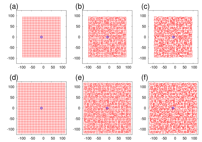
Figure 1: Network structures of aggregates for $n_{x}$=$n_{y}$=25 (a,b,c) and 31(d,e,f) cases. Disorder parameters $f$ are 0.0, 0.2 and 0.4 respectively for panel (a/d), (b/e) and (c/f). Lattice size as reference length of nearest site is $D_{x}=D_{y}=7.8$ Bohr. $f$ serves as a ratio of fluctuation compared to this reference length. Rings at the centers of panels denote the site with initial excitation.

Figure 2: Effect of disorder, mass and structure dynamics on charge migration dynamics. Top(a,d,g), middle(b,e,h) and bottom(c,f,i) panels show time dependent behaviors correspondingly of effective distance of opposite sign charges,$(d^{+}-d^{-})$ diffusion length of positive, $d^{+}$, and negative ones, $d^{-}$. Masses employed in panels in the left(a,b,c), middle(d,e,f) and right(g,h,i) columns are $\mu=5\times{10}^{4}$, $1\times{10}^{5}$ and $2\times{10}^{5}$, respectively. $n_{x}$=$n_{y}$=25.

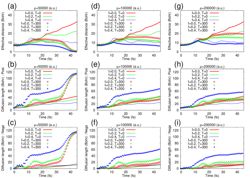
Figure 3: The counterpart of Fig.2 for $n_{x}$=$n_{y}$=31. As seen in the cases of small mass here and comparisons with small size cluster, kinematic motion affect enhancement of charge propagation

IV Concluding remarks

In this article, we numerically clarified the effect of structural disorder and dynamical fluctuation on charge migration dynamics starting from a birth of local exciton in a quantum network of molecular aggregates. For the convenient analysis, we utilized model Hamiltonians having complicate interactions of which parameters were determined by using quantum chemical calculation.

Effects of static disorder and dynamical fluctuation on charge migration were examined by varying disorder parameter, kinetic energy and effective mass of monomers. A summary of observation in the numerical part of this work is as follows: (i) structural disorder in aggregate reduces the rate of charge separation (ii) molecular motion can promote a charge diffusion in cases of smaller mass of each monomer. We can expect that these knowledge support a future realization of optimal condition for aimed properties of electronic device with respect to a charge separation leading to current in solar cell, photo catalysis reaction involved with non-local radical creation, and spontaneous photoemission caused by annihilation of electron and hole pair.

In our future work, ingredients of Hamiltonian matrix of aggregates are obtained by using, for example, the group diabatic Fock scheme gdf-eld combined with locally projection of active orbital space, consideration of non-linearity with respect to density matrix and spin-orbit interaction. rt-pgdf-eld This provides a way for exploring mechanisms underlying diffusion and migration dynamics of excition and charge density from a quantum dynamics view point, which supports a development of electronic functional material.

AVAILABILITY OF DATA

The data that support the findings of this study are available on request from the corresponding author.

Appendix A Chebyshev propagator for LVN equation

We here briefly summarize the treatment of time propagation using the Liouville–von Neumann equation of motion for a density matrix,

$$\dfrac{\partial\hat{\rho}(t)}{\partial t}=\dfrac{1}{i\hbar}\left[\hat{H},\hat{\rho}(t)\right]\equiv\dfrac{1}{i\hbar}\hat{\hat{\mathcal{L}}}\hat{\rho}(t)$$ (8)

with $\hat{\hat{\mathcal{L}}}\equiv\left[\hat{H},\hat{\rho}(t)\right]$.

An infinitesimal time propagation operator has a form of

$$\hat{\rho}(t+\Delta t)=e^{-i\hat{\hat{\mathcal{L}}}\Delta t/\hbar}\hat{\rho}(t)$$ (9)

Below we set $\hbar=1$.

The Chebyshev expansion of time propagator offering numerical stability and near uniform accuracy in the entire spectral range Guo-JCP1999-Cheby-LvN is expressed by

$$e^{-i\hat{\hat{\mathcal{L}}}\Delta t} =e^{-iL^{+}\Delta t}e^{-i\hat{\hat{\mathcal{\widetilde{L}}}}L^{-}\Delta t}$$

$$\approx e^{-iL^{+}\Delta t}\sum_{k=0}^{K}(2-\delta_{k0})I_{k}(L^{-}\Delta t)\cdot\hat{\hat{T_{k}}}\left(\hat{\hat{\mathcal{\widetilde{L}}}}\right),$$ (10)

with $L^{\pm}\equiv(L_{\textrm{max}}\pm L_{\textrm{min}})/2$ , $\hat{\hat{\mathcal{\widetilde{L}}}}\equiv(-\hat{\hat{\mathcal{L}}}+\hat{\hat{I}}L^{+})/L^{-}$ , $\hat{\hat{T_{k}}}(\hat{\hat{\mathcal{L}}})=\textrm{cos}(k\cdot\textrm{arccos}(\hat{\hat{\mathcal{L}}}))$. $L_{\textrm{max}}$ and $L_{\textrm{min}}$ are maximum and minimum eigen values. $I_{k}(x)$ is the k-th order first-kind modified Bessel function defined by $I_{k}(x)\equiv i^{-k}J_{k}(ix)$ with the k-th order first-kind Bessel function $J(x)$. The form of $J_{k}(x)$ extended from a real value variable $x$ to complex plane $z$ is expressed by $J_{k}(z)=\dfrac{1}{2\pi i}\oint e^{(z/2)(t-t^{-1})}t^{-n-1}dt$. $J_{k}(x)$ can also be defined through the Laurent expansion of $e^{(z/2)(t-t^{-1})}$ by $e^{(z/2)(t-t^{-1})}=\sum_{k=-\infty}^{\infty}J_{k}(z)t^{k}$. This also has the relation of $J_{-k}(x)=(-1)^{k}J_{k}(x)$.

Thus, the Chebyshev expansion of density operator propagated from the previous time can be written in a practical form as

$$\hat{\rho}(t+\Delta t)\approx e^{-iL^{+}\Delta t}\sum_{k=0}^{K}(2-\delta_{k0})I_{k}(L^{-}\Delta t)\hat{\rho}_{k},$$ (11)

where,

$$\hat{\rho}_{k}=2\hat{\hat{\mathcal{\widetilde{L}}}}\hat{\rho}_{k-1}-\hat{\rho}_{k-2}\quad(k\geq 2)\quad\textrm{and}$$ (12)

$$\rho_{0}\equiv\rho(t),\quad\rho_{1}\equiv\hat{\hat{\mathcal{\widetilde{L}}}}\rho(t).$$ (13)

Note that

$$\hat{\hat{\mathcal{\widetilde{L}}}}\hat{\rho}=\left[\hat{\widetilde{H}},\hat{\rho}\right]+\dfrac{L^{+}}{L^{-}}\hat{\rho}$$ (14)

with

$$\hat{\widetilde{H}}\equiv\left(-\hat{H}+\hat{I}L^{+}\right)/L^{-}$$ (15)

since

$$\hat{\hat{\mathcal{\widetilde{L}}}}\hat{\rho}=\left(-\hat{\hat{L}}+L^{+}\right)\hat{\rho}/L^{-}=\left(-\left[\hat{H},\hat{\rho}\right]+L^{+}\hat{\rho}\right)/L^{-}$$

$$= \left\{\left[(-\hat{H}),\hat{\rho}\right]+\hat{L}^{+}\hat{\rho}\right\}/L^{-}$$

$$= \left\{\left[(-\hat{H}+\hat{I}L^{+}),\hat{\rho}\right]+L^{+}\hat{\rho}\right\}/L^{-}$$

$$= \left[(-\hat{H}+\hat{I}L^{+})/L^{-},\hat{\rho}\right]+L^{+}\hat{\rho}/L^{-}$$ (16)

Here, If $L_{\textrm{max/min}}=H_{\textrm{max/min}}$ , then $L^{-}=R,L^{+}=H_{\textrm{avr}}$ with $R\equiv(H_{\textrm{max}}-H_{\textrm{min}})/2$ and $H_{avr}\equiv(H_{\textrm{max}}+H_{\textrm{min}})/2$.

$Ng=121$	$r_{\textrm{pair}}$	$N_{\textrm{st}}^{\textrm{pair}}$	CPUt	ratio
	8.8	1820	1.5	0.11
	9.8	2316	1.6	0.11
	10.8	2780	1.8	0.13
	15.8	5068	2.4	0.18
$Ng=441$	$r_{\textrm{pair}}$	$N_{\textrm{st}}^{\textrm{pair}}$	CPUt	ratio
	8.8	7028	45	0.067
	9.8	8868	45	0.067
	10.8	10998	48	0.072
	15.8	20156	58	0.087
$Ng=961$	$r_{\textrm{pair}}$	$N_{\textrm{st}}^{\textrm{pair}}$	CPUt	ratio
	8.8	15164	906	0.047
	9.8	19676	920	0.048
	10.8	24052	933	0.049
	15.8	45076	1003	0.053

Table 1: Speedup of dynamics calculation using sparsity of interaction. We presented here comparisons with respect to pair threshold distance $r_{\textrm{pair}}$ and system size $N_{\textrm{g}}$. Moderately disordered case with $f=0.5$ is used. ’CPUt’ means a CPU time took in calculations and ’ratio’ shows a ratio of CPU time in case with sparse Hamiltonian to that with full size Hamiltonian.

References

- (1) C. S. Ponseca Jr., P. Chábera Jens Uhlig, P. Persson and V. Sundström, Chem. Rev. 117, 10940 (2017).
- (2) L. Hammarström, Acc. Chem. Res. 48, 840 (2015).
- (3) M. M. Gabriel, E. M. Grumstrup, J. R. Kirschbrown, C. W. Pinion, J. D. Christesen, D. F. Zigler, E. E. M. Cating, J. F. Cahoon, and J. M. Papanikolas, Nano Lett. 14, 3079 (2014).
- (4) M. Shibuta, N. Hirata, R. Matsui, T. Eguchi, and A. Nakajima, J. Phys. Chem. Lett. 3, 981 (2012).
- (5) C. Madigan and V. Bulovic, Phys. Rev. Lett. 96, 046404 (2006).
- (6) L. E. de Sousa, P. H. de Oliveira Neto, J. K.-Hansen, and D. A. da Silva Filho, J. Chem. Phys. 148, 204101 (2018).
- (7) H. Guo, and R. Chen, J. Chem. Phys. 110 6626 (1999).
- (8) T. Yonehara and T. Nakajima, J. Chem. Phys. 147, 074110 (2017).
- (9) T. Yonehara and T. Nakajima, Chem. Phys. 528, 110508 (2020).