Landau-Zener transitions in a fermionic dissipative environment

Abstract

We study Landau-Zener transitions in a fermionic dissipative environment where a two-level (up and down states) system is coupled to two metallic leads kept with different chemical potentials at zero temperature. The dynamics of the system is simulated by an iterative numerically exact influence functional path integral method. In the pure Landau-Zener problem, two kinds of transition (from up to down state and from down to up state) probability are symmetric. However, this symmetry is destroyed by coupling the system to the bath. In addition, in both kinds of transitions, there exists a nonmonotonic dependence of the transition probability on the sweep velocity; meanwhile nonmonotonic dependence of the transition probability on the system-bath coupling strength is only shown in one of them. As in the spin-boson model, these phenomena can be explained by a simple phenomenological model.

I Introduction

In physics and chemistry, it is ubiquitous that a quantum system can be effectively described by two-level systems (TLSs). The simplest example is a particle of total spin $\frac{1}{2}$ under an external magnetic field, which can be called an “intrinsically” two-level system. A more common situation is that a system has continuous degrees of freedom which are associated with a potential with two minima Leggett et al. (1987); Weiss (1993). In 1927, Hund Hund (1927) first introduced the quantum tunneling effect when describing the intramolecular rearrangement in ammonia molecules. Soon after, Oppenheimer Oppenheimer (1928) used the tunneling effect to explain the ionization of atoms in strong electric fields. Since then quantum tunneling in isolated TLSs under external driving has been widely studied. A well-known example is the so-called Landau-Zener problem where an isolated TLS undergoes a time-dependent energy sweep. In such a model, the final transition between states of the TLS is called the Landau-Zener (LZ) transition, which was first solved independently by Landau Landau (1932), Zener Zener (1932), Stückelberg Stückelberg (1932) and Majorana Majorana (1932) in 1932.

As one of the most fundamental phenomena in quantum physics, the LZ transition plays an important role in various fields such as quantum chemistry May and Kühn (2011), atomic and molecular physics Thiel (1990); Harmin and Price (1994); Xie and Domcke (2017), solid state artificial atoms Sillanpää et al. (2006); Berns et al. (2008), spin flips in nanomagnets DeRaedt et al. (1997); Wernsdorfer (1999), quantum optics Spreeuw et al. (1990); Bouwmeester et al. (1995), Bose-Einstein condensates Witthaut et al. (2006); Zenesini et al. (2009); Olson et al. (2014), quantum information and computation Ankerhold and Grabert (2003); Izmalkov et al. (2004); Wubs et al. (2005); Oliver et al. (2005); Wei et al. (2008); Fuchs et al. (2011), and Landau-Zener-Stückelberg interferometry Shytov et al. (2003); Izmalkov et al. (2008); Shevchenko et al. (2010); Neilinger et al. (2016); Chatterjee et al. (2018); Wang et al. (2018).

For isolated TLSs, Landau-Zener transitions can be solved exactly Landau (1932); Zener (1932); Stückelberg (1932); Majorana (1932); Kayanuma (1984); Grifoni and Hänggi (1998); Wittig (2005). However, this is no longer the case when taking the environment into consideration Gefen et al. (1987); Ao and Rammer (1989, 1991) except for some limiting cases. How the environment affects the Landau-Zener transition has continuously attracted considerable attentions over the decades. Kayanuma Kayanuma (1984) proposed a simple stochastic model having a diagonal energy fluctuating term and gave the analytic LZ transition probability in the rapid fluctuation limit. Gefen et al. Gefen et al. (1987) gave a qualitative indication on how the LZ transition be affected by the environment. Ao and Rammer Ao and Rammer (1989, 1991) studied the LZ transition with an Ohmic heat bath and they found that at zero temperature in the limits of very fast and very slow sweeps the transition probability is the same as in the absence of the bath, which was confirmed by numerical calculations Kayanuma and Nakayama (1998); Kobayashi et al. (1999). Wubs et al. Wubs et al. (2005) investigated the influence of a classical radiation field on the LZ transition and obtained analytical results in the limits of large and small frequencies within a rotating wave approximation. Later they Wubs et al. (2006) gave an exact LZ transition probability for a qubit with linear coupling to a bosonic bath at zero temperature and proposed to use the LZ transition to make qubits as bath detectors. Saito et al. Saito et al. (2007) studied the LZ transition in a qubit coupled to bosonic and spin bath respectively at zero temperature and discussed their bath-specific and universal behaviors. Nalbach and Thorwart Nalbach and Thorwart (2009) studied the LZ transition in a bosonic dissipative environment by means of an iterative numerically exact influence functional path integral method, and they discover a nonmonotonic dependence of the transition probability on the sweep velocity which can be explained by a simple phenomenological model. Whitney et al. Whitney et al. (2011) found that the Lamb shift of the environment exponentially enhances the coherent oscillation amplitude in the LZ transition. Haikka and Mølmer Haikka and Mølmer (2014) studied the LZ transition when the system is subjected to continuous probing of the emitted radiation and they found the measurement back action on the system leads to significant excitation. Arceci et al. Arceci et al. (2017) revisited the issue of thermally assisted quantum annealing by a detailed study of the dissipative LZ problem in the presence of a Caldeira-Leggett bath of harmonic oscillators. Huang and Zhao Huang and Zhao (2018) employed the Dirac-Frenkel time-dependent variation to examine dynamics of the LZ problem with both diagonal and off-diagonal qubit-bath coupling.

Till now most studies of the effect of environment on the LZ transition have focused on spin-boson systems where the environment is described as a bath of harmonic oscillators. The effect of a fermionic environment is much less well understood. In this article, we employ an iterative numerically exact influence method Makarov and Makri (1994); Makri (1995); Weiss et al. (2008); Segal et al. (2010) to study LZ transitions in a fermionic environment where a TLS is coupled to two metallic leads kept with different chemical potentials at zero temperature. Such a method allows us to include nonadiabatic and non-Markovian effects and is well suited for real-time dynamics simulation of quantum dots.

In the pure LZ transition problem, two kinds of transition (from up to down state and from down to up state) probabilities are symmetric. Whether the spin is initially prepared in up state or down state, the final probability that it transits to another state is the same. According to our simulations, this is no longer the case when the system is coupled to the leads. In addition, a nonmonotonic dependence of the transition probability on the sweep velocity exists in both kinds of transition, while nonmonotonic dependence of the system-bath coupling strength is only shown in one of them. These phenomena can be explained by a simple phenomenological model as in the spin-boson model. This nonmonotonic dependence can be understood as a nontrivial competition between relaxation caused by the environment and LZ driving, and it may be useful for optimal control problems.

This article is organized as follows. The details of the model and a quick survey of the method are given in Sec. II. The simulation results and discussions are shown in Sec. III. Finally, some concluding remarks are given in Sec. IV.

II Model and Method

We consider a spin-fermion system with the time-dependent Hamiltonian

$$H(t)=H_{S}(t)+H_{B}+H_{SB},$$ (1)

where the system Hamiltonian $H_{S}(t)$ is the standard LZ Hamiltonian for an isolated TLS for which

$$H_{S}(t)=\frac{vt}{2}\sigma_{z}+\frac{\Delta_{0}}{2}\sigma_{x}$$ (2)

with the tunneling amplitude $\Delta_{0}$ and the sweep velocity $v$. Throughout this article we set $\hbar=k_{B}=1$ and use dimensionless quantities. The value of $\Delta_{0}$ is set to $\Delta_{0}^{2}=0.1$ and the value of $v$ is kept positive. $\sigma_{x}$ and $\sigma_{z}$ are Pauli matrices, and diabatic states are the eigenstates of $\sigma_{z}$ (up $\ket{\uparrow}$ and down $\ket{\downarrow}$ states). When $t\to\pm\infty$, the diabatic states coincide with the momentary eigenstates of the LZ Hamiltonian.

The bath Hamiltonian $H_{B}$ describes two independent free fermionic leads ($\alpha=L,R$ for left and right lead) for which

$$H_{B}=\sum_{\alpha k}\varepsilon_{k}c^{{\dagger}}_{\alpha k}c_{\alpha k},$$ (3)

where the operator $c^{{\dagger}}_{\alpha k}$ ($c_{\alpha k}$) creates (annihilates) an electron in the $\alpha$th lead with state $k$. These two leads are kept with a chemical potential difference $\Delta\mu$ at zero temperature. Here we suppose the chemical potential of the left lead $\mu_{L}$ is higher than that of the right lead $\mu_{R}$, and the bandwidth of both leads is taken to be $D=3$. The middle of the band is set as the zero energy point, and $\mu_{L},\mu_{R}$ are symmetrically placed on two sides of it, i.e., $\mu_{L}=\frac{1}{2}(D+\Delta\mu)$ and $\mu_{R}=\frac{1}{2}(D-\Delta\mu)$.

The system-bath coupling Hamiltonian $H_{SB}$ is taken to be

$$H_{SB}=\sum_{\alpha\beta;kq}V_{\alpha\beta}\sigma_{z}c^{{\dagger}}_{\alpha k}c_{\beta q},$$ (4)

where $\alpha,\beta$ are the bath indices. With such a system-bath coupling the momentum dependence of the scattering potential is neglected Nozières and Dominicis (1969); Ng (1995, 1996); Segal et al. (2007, 2010); Chen and Xu (2019). In particular, only interbath system-bath coupling is under consideration. Here we introduce a control parameter $\lambda$ of system-bath coupling strength for which $\rho V_{\alpha\beta}=\lambda(1-\delta_{\alpha\beta})$ , where $\rho$ is the density of states of each lead and the factor $(1-\delta_{\alpha\beta})$ ensures only interbath coupling. Fig. 1 gives a schematic representation of the model.

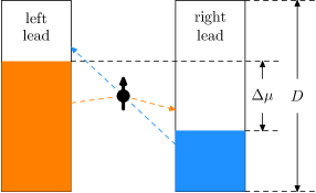
Figure 1: (Color Online) Scheme of the spin-fermion model. The two leads with bandwidth $D$ are kept with a chemical potential difference $\Delta\mu$ at zero temperature. Electrons in the leads can jump into another lead via and scattered by the spin.

In this article, we employ an iterative numerically exact influence functional path method to investigate the effects of sweep velocity $v$, system-bath coupling strength $\lambda$, and bath chemical potential $\Delta\mu$ on LZ transitions. This method is nonperturbative and allows us to include nonadiabatic and non-Markovian effects, and it is also well suited for real-time dynamics simulations of quantum dots. It was first proposed by Makarov and Makri for the time-independent spin-boson model Makarov and Makri (1994); Makri (1995). Later it was applied to the monochromatically driven spin-boson model Makarov and Makri (1995a, b); Makri and Wei (1997); Makri (1997). It was also adopted to investigate LZ transitions in the spin-boson model Nalbach and Thorwart (2009); Arceci et al. (2017).

Segal et al. generalized this method to the time-independent spin-fermion model by adopting a discretized scheme for tracing out the bath Segal et al. (2010, 2011); Simine and Segal (2013); Segal (2013); Agarwalla and Segal (2017). Chen and Xu applied this scheme to study the monochromatically driven spin-fermion model and gave a comparison between the path integral method and the Floquet master equation Chen and Xu (2019). This scheme is also adopted in this article. The basic procedure of the path integral method is as follows.

The evolution of total density matrix $\rho(t)$ is given by

$$\rho(t)=U(t)\rho(0)U^{{\dagger}}(t),$$ (5)

where

$$U(t)=\mathrm{T}\exp[-i\int_{0}^{t}H(\tau)\differential{\tau}]=\prod_{t_{i}=0}^{t}e^{-iH(t_{i})\delta t}$$ (6)

with $\mathrm{T}$ being the chronological ordering symbol. Here the product is understood as that the limit is taken over all infinitesimal interval $\delta t$ between zero and $t$ arranged from right to left in order of increasing time $t_{i}$. Employing finite $\delta t$ approximates the evolution operator $U(t)$ into a product of finite $N$ exponentials for which $U(t)\approx\prod_{i}T_{i}$, where $T_{i}=e^{-iH(t_{i})\delta t}$. Now introduce the reduced density matrix of the system $\rho_{S}=\Tr_{B}\rho$ by tracing $\rho$ over the bath degrees of freedom, which is now written as

$$\rho_{S}(s^{\prime\prime},s^{\prime};t)=\Tr_{B}[\matrixelement{s^{\prime\prime}}{T_{N}\cdots T_{1}\rho(0)T_{1}^{{\dagger}}\cdots T_{N}^{{\dagger}}}{s^{\prime}}].$$ (7)

Inserting the identity operator $\int\differential{s}\outerproduct{s}{s}$ between every two $T$ and relabeling $s^{\prime\prime},s^{\prime}$ as $s_{N}^{+},s_{N}^{-}$ gives

$$\begin{split}\rho_{S}(s_{N}^{+},s_{N}^{-};t)=&\int\differential{s_{0}}^{+}\cdots\differential{s_{N-1}^{+}}\int\differential{s_{0}^{-}}\cdots\differential{s_{N-1}^{-}}\\ &\times\Tr_{B}[\matrixelement{s_{N}^{+}}{T_{N}}{s_{N-1}^{+}}\cdots\\ &\qquad\qquad\rho(0)\cdots\matrixelement{s_{N-1}^{-}}{T_{N}^{{\dagger}}}{s_{N}^{-}}].\end{split}$$ (8)

The integrand in the above expression is referred as the “influence functional” Segal et al. (2010) (IF) which we denote by $I(s_{0}^{\pm},\ldots,s_{N}^{\pm})$. The nonlocal correlations in the IF decay exponentially under certain conditions Makarov and Makri (1994), which enables a controlled truncation of the IF. Note that for the spin-fermion system at zero temperature used in this article, the exponential decay is guaranteed by finite $\Delta\mu$ Segal et al. (2010); Weiss et al. (2008). Therefore the IF can be truncated beyond a memory time $\tau_{c}=N_{s}\delta t$ with $N_{s}$ being a positive integer and the IF can be written approximately as Makarov and Makri (1994); Makri (1995, 1999); Segal et al. (2010, 2011)

$$\begin{split}I(s_{0}^{\pm},\ldots,s_{N}^{\pm})\approx&I(s_{0}^{\pm},\ldots,s_{N_{s}}^{\pm})I_{s}(s_{1}^{\pm},\ldots,s_{N_{s}+1}^{\pm})\\ &\quad\times\cdots I_{s}(s_{N-N_{s}},\ldots,s_{N}^{\pm}),\end{split}$$ (9)

where

$$I_{s}(s_{k}^{\pm},\ldots,s_{k+N_{s}}^{\pm})=\frac{I(s_{k}^{\pm},\ldots,s_{k+N_{s}}^{\pm})}{I(s_{k}^{\pm},\ldots,s_{k+N_{s}-1}^{\pm})}.$$ (10)

In order to integrate Eq. (9) iteratively we can define a multiple time reduced density matrix $\tilde{\rho}_{S}(s_{k}^{\pm},\ldots,s_{k+N_{s}-1}^{\pm})$ with initial values $\tilde{\rho}_{S}(s_{0}^{\pm},\ldots,s_{N_{s}-1}^{\pm})=1$. Its first evolution step is given by

$$\tilde{\rho}_{S}(s_{1}^{\pm},\ldots,s_{N_{s}}^{\pm})=\int\differential{s_{0}^{\pm}}I(s_{0}^{\pm},\ldots,s_{N_{s}}^{\pm}),$$ (11)

and the latter evolution step is given by

$$\begin{split}\tilde{\rho}_{S}(s_{k+1}^{\pm},\ldots,s_{k+N_{s}}^{\pm})=&\int\differential{s_{k}^{\pm}}\tilde{\rho}_{S}(s_{k}^{\pm},\ldots,s_{k+N_{s}-1}^{\pm})\\ &\quad\times I_{s}(s_{k}^{\pm},\ldots,s_{k+N_{s}}^{\pm}).\end{split}$$ (12)

Finally the time-local ($t_{k}=k\delta t$) reduced density matrix is obtained by

$$\rho_{S}(t_{k})=\int\differential{s_{k-1}^{\pm}}\cdots\differential{s_{k-N_{s}+1}^{\pm}}\tilde{\rho}_{S}(s_{k-N_{s}+1}^{\pm},\ldots,s_{k}^{\pm}).$$ (13)

It can be seen that we need to keep track of a $2N_{s}$ rank “tensor” $\tilde{\rho}_{S}$ and a $2(N_{s}+1)$ rank “tensor” $I_{s}$. If the size of the system Hilbert space is $M$, then a space with size proportional to $M^{2N_{s}}$ is needed to store $\tilde{\rho}_{S}$ and a space with size proportional to $M^{2(N_{s}+1)}$ is needed to store $I_{s}$. The space size increases dramatically with increasing $M$ and $N_{s}$, which limits the value of time step $\delta t$, the length of $\tau_{c}$ and the size of the system $M$ in a practical calculation. However, because the method is iterative in time it is easy to deal with a time-dependent Hamiltonian.

In principle, the final results of the time-independent model can be extrapolated to the $\delta t\to 0$ limit and the error brought by finite $\delta t$ is then eliminated Segal et al. (2010); Weiss et al. (2008). However, in time-dependent driving case with different $\delta t$ the driving field is sampled in different time grids, which would bring extra error in extrapolation. In addition, $\delta t$ can not be arbitrary small with a fixed $\tau_{c}$ since we must ensure that $N_{s}$ is not too large. Therefore, as in Ref. Chen and Xu (2019), the extrapolation is not employed in this article.

III Results and Discussions

In the pure LZ problem, at initial time $t=-\infty$ the system is prepared in one diabatic state, and one seeks the probability $P_{0}$ of the system to end up in another at $t=+\infty$. If the system is initially prepared in the up state $\ket{\uparrow}$, which corresponds to the ground state, then $P_{0}$ gives the probability of the system to end up in the down state $\ket{\downarrow}$, which now also corresponds to the ground state. In other words, the LZ probability $P_{0}$ gives the final probability of the system to stay in the ground state. Similarly, if the system is initially prepared in the down state $\ket{\downarrow}$ then $P_{0}$ gives the final probability to stay in the excited state. In summary, $P_{0}$ is defined as

$$P_{0}=\absolutevalue{\matrixelement{\uparrow}{U_{S}(\infty,-\infty)}{\downarrow}}^{2}=\absolutevalue{\matrixelement{\downarrow}{U_{S}(\infty,-\infty)}{\uparrow}}^{2},$$ (14)

where $U_{S}$ is the system evolution operator

$$U_{S}(\infty,-\infty)=\mathrm{T}\exp[-i\int_{-\infty}^{\infty}H_{S}(\tau)\differential{\tau}].$$ (15)

The exact solution for $P_{0}$ is given by Landau (1932); Zener (1932); Stückelberg (1932); Majorana (1932)

$$P_{0}=1-\exp(-\frac{\pi\Delta_{0}^{2}}{2v}).$$ (16)

This solution is symmetric for both diabatic states for which whether the system is prepared in the up or down state would not affect the probability of it transiting to another diabatic state.

When the system is coupled to the environment, this symmetry is broken for which the probability of the system staying in the ground or excited state becomes different. For convenience, we denote the LZ probability of the system to stay in the ground state (corresponding to the transition from up to down state) by $P_{1}$, for which

$$P_{1}=\absolutevalue{\matrixelement{\downarrow}{U(\infty,-\infty)}{\uparrow}}^{2},$$ (17)

and the LZ probability of the system to stay in the excited state (corresponding to the transition from down to up state) by $P_{2}$, for which

$$P_{2}=\absolutevalue{\matrixelement{\uparrow}{U(\infty,-\infty)}{\downarrow}}^{2}.$$ (18)

Here $U$ denotes the total evolution operator for which

$$U(\infty,-\infty)=\mathrm{T}\exp[-i\int_{-\infty}^{\infty}H(\tau)\differential{\tau}].$$ (19)

In this section the simulation results for $P_{1}$ and $P_{2}$ are given respectively. In all figures, the simulation results are presented by dots and lines are guides for the eye.

III.1 Results of $P_{1}$

Let us first consider the case where the system is initially prepared in the up (ground) state at $t=-\infty$.

Figure 2 shows the LZ probability $P_{1}$ versus sweep velocity $v$ for weak coupling $\lambda=0.04$ and various $\Delta\mu$. It can be seen that a large velocity regime ($v\gg\Delta_{0}^{2}$) can be distinguished from a small velocity regime ($v\ll\Delta_{0}^{2}$). The result shown here is similar to that in the spin-boson model for various temperatures Nalbach and Thorwart (2009) for which larger $\Delta\mu$, which can act as a temperature like dephasing contributor Segal et al. (2007), suppresses the LZ transition more strongly. In the large-velocity regime ($v\gg\Delta_{0}^{2}$), $P_{1}$ coincides with $P_{0}$ for which little influence of the environment is shown. In the regime where $v<\Delta_{0}^{2}$, besides an overall all decrease of $P_{1}$ with increasing $\Delta\mu$, a nonmonotonic dependence of $P_{1}$ on $v$ is shown: with fixed $\Delta\mu$ and decreasing $v$, $P_{1}$ first shows a maximum at $v_{\mathrm{max}}$, which is smaller than but close to $\Delta_{0}^{2}$, then a minimum at velocity $v_{\mathrm{min}}$, and finally an increase.

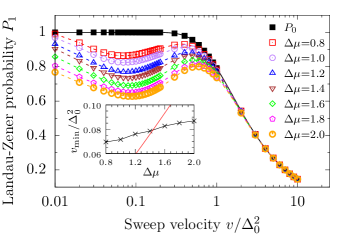
Figure 2: (Color Online) The LZ probability $P_{1}$ versus $v$ for weak system-bath coupling strength $\lambda=0.04$ and various $\Delta\mu$. Inset: $v_{\mathrm{min}}$ versus $\Delta\mu$ with same $\lambda$ as in the main figure. The simulation results are shown by black dots, and results by the phenomenological model [Eq. (23)] are shown by the red line.

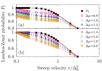
Figure 3: (Color Online) Same as Fig. 2 for larger system-bath coupling strengths (a) $\lambda=0.10$ and (b) $\lambda=0.20$.

In the spin-boson model, this nonmonotonicity can not be described by perturbative approaches but can be explained by a simple phenomenological model Nalbach and Thorwart (2009). Here we give a review on such a phenomenological model. The bath is assumed to mainly induce relaxation. At the initial time the system is prepared in the ground state; therefore only absorption can occur if an excitation with energy

$$\Delta_{t}=\sqrt{(vt)^{2}+\Delta_{0}^{2}}$$ (20)

exists in the bath spectrum and thermally populated. The quantity $\Delta_{t}$ varies with time and if it is larger than a threshold energy $\Delta_{c}$ then relaxation would stop. In other words, relaxation can only occur within a time window from $-\frac{1}{2}t_{r}$ to $\frac{1}{2}t_{r}$, where

$$t_{r}=\frac{2}{v}\sqrt{\Delta_{c}^{2}-\Delta_{0}^{2}}.$$ (21)

The threshold energy $\Delta_{c}$ is taken to be the smaller of the temperature $T$ and the bath cutoff frequency $\omega_{c}$. Let $\tau_{r}$ denote the system relaxation time; then $\tau_{r}$ must be shorter than $t_{r}$ for relaxation processes to contribute.

When the sweep velocity $v$ is large, $t_{r}$ is small for which $t_{r}\ll\tau_{r}$; therefore relaxation can not occur and the bath has little influence on the LZ transition for which $P_{1}$ coincides with $P_{0}$. In the opposite limit where $v\to 0$ for which $t_{r}\gg\tau_{r}$, the system will get full relaxation at any time according to momentary Hamiltonian. Since relaxation stops at the threshold energy, the system would be adjusted according to $\Delta_{c}$ and $T$. For small but finite sweep velocity, equilibration is retarded for which the system is relaxed according to the past momentary Hamiltonian. The system is then assumed to be equilibrated toward a time-averaged energy splitting

$$\bar{\Delta}_{r}=\frac{1}{t_{r}}\int_{-t_{r}/2}^{t_{r}/2}\Delta_{t}\differential{t},$$ (22)

leading to $P_{1}(v_{\mathrm{min}})=\frac{1}{2}[1+\tanh(\bar{\Delta}_{r}/2T)]$.

According to the discussion, large $t_{r}$ or small $t_{r}$ would weaken the suppression of the LZ transition. Thus it is assumed that relaxation will maximally suppress the LZ transition when $t_{r}$ and $\tau_{r}$ coincide,

$$t_{r}(v_{\mathrm{min}})=\tau_{r},$$ (23)

which leads to a minimum of $P_{1}$ at $v_{\mathrm{min}}$. If only single-phonon absorption is considered within resonance ($\absolutevalue{t}\leq\frac{t_{r}}{2}$), then the system relaxation time $\tau_{r}$ can estimated by the golden rule with time-averaged energy splitting $\bar{\Delta}_{r}$ for which

$$\tau_{r}^{-1}=\pi\alpha\frac{\Delta_{0}^{2}}{\bar{\Delta}_{r}}\exp(-\bar{\Delta}_{r}/\omega_{c})n(\bar{\Delta}_{r}),$$ (24)

where $\alpha$ is the system-bath coupling strength and $n(\bar{\Delta}_{r})$ is the Bose-Einstein distribution function. A revisit of the golden rule used in the spin-boson model is given in the Appendix. Comparing Eq. (21) and (24) gives the position of $v_{\mathrm{min}}$.

Now apply this phenomenological model to our spin-fermion model. Since the system is prepared in the ground state, only absorption can occur if an electron jumps from the left lead to an unoccupied state with lower energy in the right lead. The energy difference of the electron before and after the jump should be $\Delta_{t}$. The largest energy change by the jump is $\Delta\mu$ (when an electron at the Fermi level in the left lead jump to the Fermi level of the right lead); thus $\Delta_{c}=\Delta\mu$.

When the sweep velocity $v$ is large for which $t_{r}\ll\tau_{r}$, the relaxation can not occur and thus $P_{1}$ coincides with $P_{0}$. When the sweep velocity $v$ is small for which $t_{r}\gg\tau_{r}$, the system would be fully relaxed according to $\Delta_{c}=\Delta\mu$ at zero temperature. In the spin-fermion model, the full relaxation of the system is determined not by the temperature but by the chemical potential difference $\Delta\mu$. According to Ref. Segal et al. (2007), it has no simple analytical formula for the system polarization $\expectationvalue{\sigma_{z}}$, but it is known that $\expectationvalue{\sigma_{z}}$ manifests a transition from a fully polarized system, where the system is in the ground state, to an unpolarized system, where $\expectationvalue{\sigma_{z}}=0$ as $\Delta\mu$ increases. Since $\Delta_{c}=\Delta\mu$, which is equivalent to say $\Delta\mu$ is not large, after fully relaxation the system would be adjusted to the ground state. Therefore $P_{1}=1$ when $v\to 0$, and this can be seen more clearly from Fig. 3(b) where a larger coupling strength $\lambda$ accelerates relaxation processes.

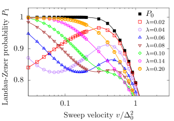
Figure 4: (Color Online) The LZ probability $P_{1}$ versus $v$ for $\Delta\mu=1.0$ and various $\lambda$.

When $t_{r}$ matches $\tau_{r}$, the relaxation maximally suppresses the LZ transition, which gives a minimum at $v_{\mathrm{min}}$. Since the value of $P_{1}(v_{\mathrm{min}})$ must be smaller than $P_{1}(v\to 0)=1$, as $v\to 0$ the probability $P_{1}$ must increase again with decreasing $v$. Therefore $P_{1}$ shows a maximum at $v_{\mathrm{max}}$, and minimum at $v_{\mathrm{min}}$, and then an increase with decreasing $v$, as shown in Fig. 2. Basically, the mechanism for nonmonotonic dependence on $v$ in the spin-fermion model is same as that in the spin-boson model. If the system ends up in an unpolarized state with $\expectationvalue{\sigma_{z}}=0$ then we have $P_{1}=\frac{1}{2}$. This is the reason why $P_{1}(v_{\mathrm{min}})$ deviates from $P_{0}$ and is closer to $\frac{1}{2}$ for larger $\Delta\mu$, or in other words, larger $\Delta\mu$ would suppress the LZ transition more strongly.

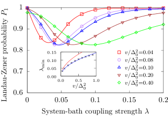
Figure 5: (Color Online) The LZ probability $P_{1}$ versus $\lambda$ for $\Delta\mu=1.0$ and various $v$. Inset: $\lambda_{\mathrm{min}}$ versus $v$ with same $\Delta\mu$ in the main figure. The simulation data are shown by black dots, results by the phenomenological model are shown by the red line, and the blue line represents a fitting function $y=0.145x^{\frac{1}{2}}$.

For a fixed time and weak coupling, the decay rate out of the ground state can be estimated by the golden rule if only a single electron jump is considered. After summing up all possible jumps whose energy difference is $\Delta_{t}$, we obtain the decay rate as (see the Appendix)

$$\tau^{-1}=2\pi\lambda^{2}\frac{\Delta_{0}^{2}}{\Delta_{t}^{2}}(\Delta\mu-\Delta_{t}).$$ (25)

In the spin-boson model, $\tau_{r}^{-1}$ is archived via simply substituting $\Delta_{t}$ by $\bar{\Delta}_{r}$ in the expression of $\tau^{-1}$. However, in the spin-fermion model, due to the inverse quadratic dependence on $\Delta_{t}$ of $\tau^{-1}$, it would be more appropriate to estimate $\tau_{r}^{-1}$ by the time-averaged decay rate

$$\begin{split}\tau_{r}^{-1}&=\frac{1}{t_{r}}\int_{-t_{r}/2}^{t_{r}/2}2\pi\lambda^{2}\frac{\Delta_{0}^{2}}{\Delta_{t}^{2}}(\Delta\mu-\Delta_{t})\differential{t}\\ &=\frac{4\pi}{vt_{r}}\lambda^{2}\Delta_{0}^{2}\quantity[\frac{\Delta\mu}{\Delta_{0}}\atan(\frac{vt_{r}}{2\Delta_{0}})-\mathrm{asinh}(\frac{vt_{r}}{2\Delta_{0}})].\\ \end{split}$$ (26)

This formula predicts that $v_{\mathrm{min}}$ increases almost linearly with increasing $\Delta\mu$ when $\Delta_{c}\gg\Delta_{0}$. The positions of $v_{\mathrm{min}}$ versus $\Delta\mu$ for $\lambda=0.04$ is shown in the inset of Fig. 2. It can be seen that $v_{\mathrm{min}}$ roughly shows a linearly dependence on $\Delta\mu$. However, employing Eq. (23) we have $v_{\mathrm{min}}\approx 0.043\Delta_{0}^{2}$ for $\Delta\mu=1.0$ and $v_{\mathrm{min}}\approx 0.127\Delta_{0}^{2}$ for $\Delta\mu=2.0$. This result only qualitatively agrees with what is shown in Fig. 2 where $v_{\mathrm{min}}\approx 0.072\Delta_{0}^{2}$ for $\Delta\mu=1.0$ and $v_{\mathrm{min}}\approx 0.087\Delta_{0}^{2}$ for $\Delta\mu=2.0$.

Figure 3 shows the LZ transition probability $P_{1}$ versus sweep velocity $v$ for larger $\lambda$ and various $\Delta\mu$. As seen from Eq. (26), the relaxation rate is proportional to $\lambda^{2}$ for which increasing $\lambda$ enhances relaxation and decreases $\tau_{r}$ accordingly. For $\lambda=0.1$ [Fig. 3(a)] the minimum disappears and only a shoulder remains. For $\lambda=0.2$ [Fig. 3(b)], only a monotonic growth of $P_{1}$ with decreasing $v$ remains, and the relaxation processes are greatly accelerated for which at $v/\Delta_{0}^{2}=0.1$ the LZ transition probabilities $P_{1}$ already reduce to 1.

Figure 4 shows the LZ transition probability $P_{1}$ versus $v$ for $\Delta\mu=1.0$ and various $\lambda$. For small $\lambda=0.04,0.06,0.08$, the minimum $P_{1}(v_{\mathrm{min}})$ can be still observed and $v_{\mathrm{min}}$ shifts to larger velocity for increasing $\lambda$. The minimum disappears when $\lambda\geq 0.10$ and in this case $P_{1}$ goes to 1 for small $v$. Due to these features, the lines of $P_{1}$ in Fig. 4 have cross points, which means there is a nonmonotonic dependence of $P_{1}$ on $\lambda$. This can be seen more clearly in Fig. 5.

Figure 5 shows the dependence of $P_{1}$ on $\lambda$ for $\Delta\mu=1.0$ and various $v$. It can be seen that $P_{1}$ shows a minimum at $\lambda_{\mathrm{min}}$ for a fixed $v$. Since $t_{r}^{-1}\propto v$ and $\tau_{r}^{-1}\propto\lambda^{2}$, we have $\lambda_{\mathrm{min}}^{2}\propto v$ which means there is a simple quadratic dependence between $v$ and $\lambda_{\mathrm{min}}$: when $v$ is scaled by a factor of $a$ then $\lambda_{\mathrm{min}}$ would be scaled by a factor of $\sqrt{a}$. This conclusion agrees with the results shown in the inset of the figure where a inverse quadratic fitting is shown.

Equation (26) gives a simple description of the effect of $\lambda$ on $\tau_{r}^{-1}$, while the effect of $\Delta\mu$ is much more complex. It is because $\Delta\mu$ plays a role as both temperature $T$ and bath cutoff frequency $\omega_{c}$ in the spin-boson model, which makes its effect on the relaxation complex, while larger $\lambda$ simply enhances the relaxation. In the spin-boson model, it is already mentioned that by the phenomenological picture the behavior of the crossover temperature can be only roughly described with absolute values off by a factor of 3 Nalbach and Thorwart (2009). This may be the reason why the results of Eq. (26) always have some deviations from simulation data since the effect of $\omega_{c}$ can not be removed from $\Delta\mu$.

III.2 Results of $P_{2}$

Now let us turn to $P_{2}$ which stands for the LZ transition probability from down to up state, where the system is prepared in the excited state at $t=-\infty$.

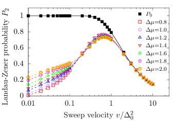
Figure 6: (Color Online) The LZ probability $P_{2}$ versus $v$ for weak system-bath coupling strength $\lambda=0.04$ and various $\Delta\mu$.

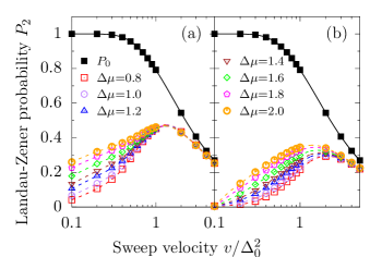
Figure 7: (Color Online) The same as Fig. 6 for larger system-bath coupling strengths (a) $\lambda=0.10$ and (b) $\lambda=0.20$.

Figure 6 shows the LZ probability $P_{2}$ versus $v$ for weak coupling $\lambda=0.04$ and various $\Delta\mu$. In large sweep velocity regime ($v\gg\Delta_{0}^{2}$), since $t_{r}$ is too short for relaxation $P_{2}$ coincides with $P_{0}$, just like $P_{1}$. In the small sweep velocity regime ($v\ll\Delta_{0}^{2}$), there is great difference between the behaviors of $P_{2}$ and $P_{1}$. For small $v$, $P_{1}$ is close to $P_{0}$, i.e., close to 1, while $P_{2}$ is far away from $P_{0}$ and close to zero. With fixed $\Delta\mu$ and decreasing $v$, $P_{2}$ shows a maximum at $v_{\mathrm{max}}$, which is smaller than but close to $\Delta_{0}^{2}$, then decreases all along and no minimum is shown.

Although behaviors of $P_{1}$ and $P_{2}$ differ greatly for small $v$, they are due to the same relaxation mechanism. For $P_{1}$, we are seeking the probability of the system to stay in the ground state, while for $P_{2}$, the probability of the system to stay in the excited state is desired. However, when $v$ is small a full relaxation would lead the system towards the ground state, and this makes $P_{1}$ go to 1 and $P_{2}$ to zero.

There is another difference between the behaviors of $P_{1}$ and $P_{2}$ in the small-$v$ regime: for $P_{1}$, larger $\Delta\mu$ suppresses the LZ transition probability more strongly, while for $P_{2}$, larger $\Delta\mu$ increases the LZ transition probability instead. This is because, as mentioned earlier, larger $\Delta\mu$ would relax the system toward an unpolarized state, where $\expectationvalue{\sigma_{z}}=0$, which makes $P_{2}$ closer to $\frac{1}{2}$. Around $v_{\mathrm{max}}$, the situation is in another way around for which larger $\Delta\mu$ decreases $P_{2}$. The underlying reason is the same: larger $\Delta\mu$ makes the system go toward an unpolarized state, i.e., makes $P_{2}$ closer to $\frac{1}{2}$.

Since the system is initially prepared in the excited state, only emission can occur within resonance ($\absolutevalue{t}\leq\frac{t_{r}}{2}$). In the emission process, there are two kinds jumping: an electron in the left lead jumps to an unoccupied state with higher energy in the right lead, and an electron in the right lead jumps to an unoccupied state in the left lead with higher energy. The energy difference by the jump should be $\Delta_{t}$. If only a single electron jump is considered, the golden rule formula for the decay rate out of the excited state is given in the Appendix. Basically, the golden rule states that the decay rate $\tau^{-1}$ has a quadratic dependence on $\lambda$ as in the absorption process, while its dependence on $\Delta\mu$ is of more complexity.

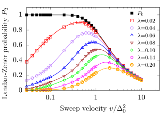
Figure 8: (Color Online) The LZ probability $P_{2}$ versus $v$ for $\Delta\mu=1.0$ and various $\lambda$.

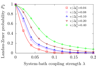
Figure 9: (Color Online) The LZ probability $P_{2}$ versus $\lambda$ for $\Delta\mu=1.0$ and various $v$.

Figure 7 shows the same content as Fig. 6 for larger system-bath coupling strengths. Since the relaxation rate is proportional to $\lambda^{2}$, larger $\lambda$ accelerates relaxation and decreases $\tau_{r}$. It can be seen that with $\Delta\mu=2.0$ when $\lambda=0.04$ (Fig. 6) $P_{2}$ is close to 0.2 at $v=0.01\Delta_{0}^{2}$, while when $\lambda=0.1$ [Fig. 7(b)] $P_{2}$ is already close to 0.2 at $v=0.1\Delta_{0}^{2}$. For $\lambda=0.2$ [Fig. 7(b)], $P_{2}$ already reduces to zero at $v=0.1\Delta_{0}^{2}$.

Figure 8 shows the LZ transition probability $P_{2}$ versus $v$ for $\Delta\mu=1.0$ and various $\lambda$. Unlike $P_{1}$ shown in Fig. 4, lines of $P_{2}$ in Fig. 8 have no cross points. This is because there is no $v_{\mathrm{min}}$ in $P_{2}$. In addition, due to the same reason the dependence of $\lambda$ of $P_{2}$ becomes monotonic. This can be seen from Fig. 9 which shows $P_{2}$ versus $\lambda$ for $\Delta\mu=1.0$ and various $v$. It can be seen that larger $\lambda$ accelerates the relaxation and makes $P_{2}$ go to zero, and smaller $v$ also enhances the relaxation.

IV Conclusions

We have studied LZ transitions in a fermionic environment where a TLS is coupled to two metallic leads kept with different chemical potential at zero temperature. The dynamics of the system is simulated by an iterative numerically exact influence functional path integral method which allows us to include nonadiabatic and non-Markovian effects.

The LZ transition probability is the probability of the system staying in the ground (excited) state $P_{1}$ ($P_{2}$) after an energy sweep. In the pure LZ problem, the two kinds of probability are symmetric; i.e., they are the same no matter whether the system is initially prepared in the ground or excited state.

The symmetry no longer exists after taking the effect of the environment into consideration. In the large sweep velocity regime, $v\gg\Delta_{0}^{2}$, since the resonance time $t_{r}$ is much shorter than the system relaxation time $\tau_{r}$, the bath has little influence on the transition; thus both $P_{1}$ and $P_{2}$ coincide with the pure LZ transition probability $P_{0}$. In the small sweep velocity regime, $v\ll\Delta_{0}^{2}$, the system is fully relaxed to the ground state, which makes $P_{1}$ go to 1 and $P_{2}$ to zero. This is the reason why the symmetry no longer exists. Due to the same reason, $P_{1}$ shows a minimum at $v_{\mathrm{min}}$ and $\lambda_{\mathrm{min}}$, while $P_{2}$ shows no minimum.

According to the phenomenological model, the existence of $v_{\mathrm{min}}$ of $P_{1}$ is understood as a nontrivial competition between relaxation and LZ driving, where the LZ transition is maximally suppressed when the resonance time $t_{r}$ and the system relaxation time $\tau_{r}$ coincide. The system relaxation time $\tau_{r}$ can be estimated by the golden rule, which states that $\tau_{r}^{-1}$ has a quadratic dependence on the system-bath coupling strength $\lambda$. This statement agrees with our results, which indicates that the effect of $\lambda$ is fairly simple.

The effect of $\Delta\mu$ on the dissipation is of more complexity. If we treat $\Delta\mu$ as the temperature, then results similar to those shown in Figs. 2, 3, and 4 can be found in the LZ transitions in the spin-boson model Nalbach and Thorwart (2009). This is because $\Delta\mu$ can act as a temperature like dephasing contributor. However, it is not really the temperature and the temperature also has its own effect on the LZ transitions. At zero temperature, the system manifests a transition from the ground state to an unpolarized system as $\Delta\mu$ increases. This means that when the value of $\Delta_{t}$ can compare with $\Delta\mu$, then the system would be relaxed to the ground state. Meanwhile in the spin-boson model, the system would not be relaxed to the ground state at finite temperature, and the bath shows no effect on the LZ probability when the system and bath are diagonally coupled at zero temperature Wubs et al. (2006).

In addition, $\Delta\mu$ also plays the role of the cutoff frequency $\omega_{c}$ of the spin-boson model, where the effect of $\omega_{c}$ can be also only qualitatively described by the phenomenological model. The dual role of $\Delta\mu$ as both the temperature $T$ and the cutoff frequency $\omega_{c}$ in the spin-boson model makes its effect on the dissipation complex. This may be the reason why results by the phenomenological model always have some deviations from simulation data since the effect of $\omega_{c}$ can not be removed from $\Delta\mu$. The interplay between the external field, system-bath coupling $\lambda$ and chemical potential difference $\Delta\mu$ remains open for further investigations.

Despite the different effects of the bosonic and fermionic baths discussed above, the phenomenological model also gives some universal predictions despite what kind of environment is present: when the sweep velocity is large, due to small relaxation time window $t_{r}$ the effect of the environment can be neglected; when the sweep velocity is small, the system would be fully relaxed according to the environment, where the environment shows its characteristics most; in the intermediate sweep velocity regime, the LZ probability shows a nonmonotonic dependence on the sweep velocity and the coupling parameter. This nonmonotonic feature may be useful for optimal control problems and for further experiments.

Appendix A Golden Rule

In this appendix, we shall revisit the derivation of the golden rule formula used for the LZ transition in the spin-boson model Nalbach and Thorwart (2009), and then following the same spirit we shall derive the golden rule for the spin-fermion model studied in this article.

A.1 Spin-Boson Model

The Hamiltonian of the spin-boson model is

$$H=H_{S}+H_{B}+H_{SB},$$ (27)

where the system and bath Hamiltonian are

$$H_{S}=\frac{\varepsilon}{2}\sigma_{z}+\frac{\Delta_{0}}{2},\quad H_{B}=\sum_{k}\omega_{k}b_{k}^{{\dagger}}b_{k}.$$ (28)

Here $\varepsilon$ and $\Delta_{0}$ are level splitting and tunneling amplitude of the TLS, respectively, and $b_{k}$ ($b_{k}^{{\dagger}}$) are bosonic annihilation (creation) operators. For simplicity we assume $\varepsilon$ is positive. The system-bath coupling is written as

$$H_{SB}=\frac{\sigma_{z}}{2}\sum_{k}\lambda_{k}(b_{k}+b_{k}^{{\dagger}}),$$ (29)

and the bath influence is described by the spectral density

$$J(\omega)=\sum_{k}\lambda_{k}^{2}\delta(\omega-\omega_{k})=2\alpha\omega\exp(-\omega/\omega_{c}),$$ (30)

where an Ohmic form with cutoff frequency $\omega_{c}$ and coupling strength $\alpha$ is considered.

The system Hamiltonian $H_{S}$ can be diagonalized by an unitary rotation for which

$$\bar{H}_{S}=e^{\frac{1}{2}i\theta\sigma_{y}}H_{S}e^{-\frac{1}{2}i\theta\sigma_{y}}=\frac{1}{2}\Delta_{t}\sigma_{z}$$ (31)

when $\tan\theta=\Delta_{0}/\varepsilon$, where $\Delta_{t}=\sqrt{\varepsilon^{2}+\Delta_{0}^{2}}$. After the rotation, the system-bath coupling becomes

$$\bar{H}_{SB}=\frac{1}{2\Delta_{t}}(\varepsilon\sigma_{z}-\Delta_{0}\sigma_{x})\sum_{k}\lambda_{k}(b_{k}+b_{k}^{{\dagger}}).$$ (32)

The Pauli matrix $\sigma_{x}$ can be written in terms of $\sigma_{+}=\frac{1}{2}(\sigma_{x}+i\sigma_{y})$ and $\sigma_{-}=\frac{1}{2}(\sigma_{x}-i\sigma_{y})$ for which $\sigma_{x}=\sigma_{+}+\sigma_{-}$. If only a single phonon absorption is considered in the absorption process, then in $\bar{H}_{SB}$ only the term $\frac{1}{2}\frac{\Delta_{0}}{\Delta_{t}}\sum_{k}\sigma_{+}b_{k}$ is relevant. Let $\ket{1}$ denote the excited state ($\sigma_{z}=+1$) and $\ket{2}$ denote the ground state ($\sigma_{z}=-1$), and let $\ket{n_{k}}$ denote the phonon state $\frac{1}{\sqrt{n_{k}!}}(b_{k}^{{\dagger}})^{n_{k}}\ket{0}$, where $\ket{0}$ is the vacuum state. Then starting from the state $\ket{2}$, the probability $p(t)$ of the system to go to the state $\ket{1}$ at time $t$ is given by the golden rule formula Leggett et al. (1987); Weiss (1993)

$$\begin{split}p(t)=&\frac{1}{4}\frac{\Delta_{0}^{2}}{\Delta_{t}^{2}}\int_{0}^{t}\int_{0}^{t}\sum_{k}\rho_{k}\lambda_{k}^{2}e^{i(\Delta_{t}-\omega_{k})(t_{1}-t_{2})}\\ &\quad\times\absolutevalue{\matrixelement{1}{\sigma_{+}}{2}\matrixelement{n_{k}-1}{b_{k}}{n_{k}}}^{2}\differential{t_{1}}\differential{t_{2}},\end{split}$$ (33)

where $\rho_{k}$ is the Gibbs distribution function

$$\rho_{k}=\exp(-\frac{n_{k}\omega_{k}}{T})/\sum_{n_{k}}\exp(-\frac{n_{k}\omega_{k}}{T})$$ (34)

with temperature $T$. If the integrand in Eq. (33) dies sufficiently fast as a function of $(t_{1}-t_{2})$, then the decay rate of the system out of the state $\ket{2}$ can be defined as

$$\begin{split}\tau^{-1}&=\frac{1}{4}\frac{\Delta_{0}^{2}}{\Delta_{t}^{2}}\int_{-\infty}^{\infty}\sum_{k}\lambda_{k}^{2}e^{i(\Delta_{t}-\omega_{k})t}n(\omega_{k})\differential{t}\\ &=\frac{1}{4}\frac{\Delta_{0}^{2}}{\Delta_{t}^{2}}\sum_{k}2\pi\lambda_{k}^{2}\delta(\Delta_{t}-\omega_{k})n(\omega_{k})\\ &=\pi\alpha\frac{\Delta_{0}^{2}}{\Delta_{t}}\exp(-\Delta_{t}/\omega_{c})n(\Delta_{t}),\end{split}$$ (35)

where $n(\omega)=(e^{\beta\omega}-1)^{-1}$ is the Bose-Einstein distribution function.

Similarly, if only a single phonon emission is considered in the emission process then in $\bar{H}_{SB}$ only the term $\frac{1}{2}\frac{\Delta_{0}}{\Delta_{t}}\sum_{k}\sigma_{-}b_{k}^{{\dagger}}$. Therefore the decay rate of the system out of the state $\ket{1}$ is

$$\tau^{-1}=\pi\alpha\frac{\Delta_{0}^{2}}{\Delta_{t}}\exp(-\Delta_{t}/\omega_{c})[1+n(\Delta_{t})].$$ (36)

From Eq. (35) and (36) it can be seen that at zero temperature the decay rate out of the ground state is zero, while the decay rate out of the excited state remains finite, as they should be.

A.2 Spin-Fermion Model

In the spin-fermion model, for a fixed time $t$, denoting $vt$ in Eq. (2) by $\varepsilon$ yields

$$H_{S}=\frac{\varepsilon}{2}\sigma_{z}+\frac{\Delta_{0}}{2}\sigma_{x}.$$ (37)

For simplicity, we assume $\varepsilon$ is positive. This $H_{S}$ can be diagonalized by the same rotation as in Eq. (31). Let $\Delta_{t}=\sqrt{\varepsilon^{2}+\Delta_{0}^{2}}$; then after the rotation the system-bath coupling becomes

$$\bar{H}_{SB}=\frac{1}{\Delta_{t}}\sum_{\alpha\beta;kq}V_{\alpha\beta}(\varepsilon\sigma_{z}-\Delta_{0}\sigma_{x})c^{{\dagger}}_{\alpha k}c_{\beta q}.$$ (38)

Similarly, we can write $\sigma_{x}$ in terms of $\sigma_{+}$ and $\sigma_{-}$ as $\sigma_{x}=\sigma_{+}+\sigma_{-}$. In the absorption process, if only a single electron jump is considered then only jumps from the left lead to an unoccupied state with lower energy in the right lead are permitted. The energy difference of the electron before and after jump should be $\Delta_{t}$. Therefore in $\bar{H}_{SB}$ only the term $\frac{1}{\Delta_{t}}\sum_{kq}V_{RL}\sigma_{+}c_{Rq}^{{\dagger}}c_{Lk}$ is relevant, and the golden rule formula for the decay rate of the system out of the ground state can be written as

$$\tau^{-1}=2\pi\lambda^{2}\frac{\Delta_{0}^{2}}{\Delta_{t}^{2}}(\Delta\mu-\Delta_{t})$$ (39)

for $\Delta_{t}\leq\Delta\mu$. When $\Delta_{t}>\Delta\mu$, the decay rate becomes zero; thus we have $\Delta_{c}=\Delta\mu$.

The situation is more complex in the emission process. Two kinds jumping are allowed: an electron in the left lead jumps to an unoccupied state with higher energy in the right lead (the term $\frac{1}{\Delta_{t}}\sum_{kq}V_{RL}c_{Rk}^{{\dagger}}c_{Lq}$ in $\bar{H}_{SB}$ is involved), and an electron in the right lead jumps to an unoccupied state in the left lead (the term $\frac{1}{\Delta_{t}}\sum_{kq}V_{LR}c_{Lk}^{{\dagger}}c_{Rq}$ in $\bar{H}_{SB}$ is involved). The energy difference before and after the jump should be $\Delta_{t}$. After summing up all possible jumps, the decay rate in the former jump can be identified as

$$\tau^{-1}=2\pi\lambda^{2}\frac{\Delta_{0}^{2}}{\Delta_{t}^{2}}\Delta\mu$$ (40)

for $\Delta_{0}\leq\Delta_{t}\leq\frac{1}{2}(D-\Delta\mu)$ and

$$\tau^{-1}=2\pi\lambda^{2}\frac{\Delta_{0}^{2}}{\Delta_{t}^{2}}[\frac{1}{2}(D+\Delta\mu)-\Delta_{t}]$$ (41)

for $\frac{1}{2}(D-\Delta\mu)<\Delta_{t}\leq\frac{1}{2}(D+\Delta\mu)$. The decay rate in the latter jump is

$$\tau^{-1}=2\pi\lambda^{2}\frac{\Delta_{0}^{2}}{\Delta_{t}^{2}}(\Delta_{t}-\Delta\mu)$$ (42)

for $\Delta\mu<\Delta_{t}\leq D$. The decay rate becomes zero under other conditions; therefore $\Delta_{c}=D$.

References

- Leggett et al. (1987) A. J. Leggett, S. Chakravarty, A. T. Dorsey, M. P. A. Fisher, A. Garg, and W. Zwerger, Reviews of Modern Physics 59, 1 (1987).
- Weiss (1993) U. Weiss, Quantum Dissipative Systems (World Scientific, Singapore, 1993).
- Hund (1927) F. Hund, Zeitschrift fur Physik 43, 805 (1927).
- Oppenheimer (1928) J. R. Oppenheimer, Physical Review 31, 66 (1928).
- Landau (1932) L. D. Landau, Physikalische Zeitschrift der Sowjetunion 2, 46 (1932).
- Zener (1932) C. Zener, Proceedings of the Royal Society A 137, 696 (1932).
- Stückelberg (1932) E. Stückelberg, Helvetica Physica Acta 5, 369 (1932).
- Majorana (1932) E. Majorana, Nuovo Cimento 9, 43 (1932).
- May and Kühn (2011) V. May and O. Kühn, Charge and Energy Transfer Dynamics in Molecular Systems (Wiley-VCH verlag, Berlin, 2011).
- Thiel (1990) A. Thiel, Journal of Physics G: Nuclear and Particle Physics 16, 867 (1990).
- Harmin and Price (1994) D. A. Harmin and P. N. Price, Physical Review A 49, 1933 (1994).
- Xie and Domcke (2017) W. Xie and W. Domcke, The Journal of Chemical Physics 147, 184114 (2017).
- Sillanpää et al. (2006) M. Sillanpää, T. Lehtinen, A. Paila, Y. Makhlin, and P. Hakonen, Physical Review Letters 96, 187002 (2006).
- Berns et al. (2008) D. M. Berns, M. S. Rudner, S. O. Valenzuela, K. K. Berggren, W. D. Oliver, L. S. Levitov, and T. P. Orlando, Nature 455, 51 (2008).
- DeRaedt et al. (1997) H. DeRaedt, S. Miyashita, K. Saito, D. García-Pablos, and N. García, Physical Review B 56, 11761 (1997).
- Wernsdorfer (1999) W. Wernsdorfer, Science 284, 133 (1999).
- Spreeuw et al. (1990) R. J. C. Spreeuw, N. J. van Druten, M. W. Beijersbergen, E. R. Eliel, and J. P. Woerdman, Physical Review Letters 65, 2642 (1990).
- Bouwmeester et al. (1995) D. Bouwmeester, N. H. Dekker, F. E. v. Dorsselaer, C. A. Schrama, P. M. Visser, and J. P. Woerdman, Physical Review A 51, 646 (1995).
- Witthaut et al. (2006) D. Witthaut, E. M. Graefe, and H. J. Korsch, Physical Review A 73, 063609 (2006).
- Zenesini et al. (2009) A. Zenesini, H. Lignier, G. Tayebirad, J. Radogostowicz, D. Ciampini, R. Mannella, S. Wimberger, O. Morsch, and E. Arimondo, Physical Review Letters 103, 090403 (2009).
- Olson et al. (2014) A. J. Olson, S.-J. Wang, R. J. Niffenegger, C.-H. Li, C. H. Greene, and Y. P. Chen, Physical Review A 90, 013616 (2014).
- Ankerhold and Grabert (2003) J. Ankerhold and H. Grabert, Physical Review Letters 91, 016803 (2003).
- Izmalkov et al. (2004) A. Izmalkov, M. Grajcar, E. Il’ichev, N. Oukhanski, T. Wagner, H.-G. Meyer, W. Krech, M. H. S. Amin, A. M. van den Brink, and A. M. Zagoskin, Europhysics Letters 65, 844 (2004).
- Wubs et al. (2005) M. Wubs, K. Saito, S. Kohler, Y. Kayanuma, and P. Hänggi, New Journal of Physics 7, 218 (2005).
- Oliver et al. (2005) W. D. Oliver, Y. Yu, J. C. Lee, K. K. Berggren, L. S. Levitov, and T. P. Orlando, Science 310, 1653 (2005).
- Wei et al. (2008) L. F. Wei, J. R. Johansson, L. X. Cen, S. Ashhab, and F. Nori, Physical Review Letters 100, 113601 (2008).
- Fuchs et al. (2011) G. D. Fuchs, G. Burkard, P. V. Klimov, and D. D. Awschalom, Nature Physics 7, 789 (2011).
- Shytov et al. (2003) A. V. Shytov, D. A. Ivanov, and M. V. Feigel’man, The European Physical Journal B 36, 263 (2003).
- Izmalkov et al. (2008) A. Izmalkov, S. H. W. van der Ploeg, S. N. Shevchenko, M. Grajcar, E. Il’ichev, U. Hübner, A. N. Omelyanchouk, and H.-G. Meyer, Physical Review Letters 101, 017003 (2008).
- Shevchenko et al. (2010) S. Shevchenko, S. Ashhab, and F. Nori, Physics Reports 492, 1 (2010).
- Neilinger et al. (2016) P. Neilinger, S. N. Shevchenko, J. Bogár, M. Rehák, G. Oelsner, D. S. Karpov, U. Hübner, O. Astafiev, M. Grajcar, and E. Il’ichev, Physical Review B 94, 094519 (2016).
- Chatterjee et al. (2018) A. Chatterjee, S. N. Shevchenko, S. Barraud, R. M. Otxoa, F. Nori, J. J. L. Morton, and M. F. Gonzalez-Zalba, Physical Review B 97, 045405 (2018).
- Wang et al. (2018) Z. Wang, W. C. Huang, Q. F. Liang, and X. Hu, Scientific Reports 8, 7920 (2018).
- Kayanuma (1984) Y. Kayanuma, Journal of the Physical Society of Japan 53, 108 (1984).
- Grifoni and Hänggi (1998) M. Grifoni and P. Hänggi, Physics Reports 304, 229 (1998).
- Wittig (2005) C. Wittig, The Journal of Physical Chemistry B 109, 8428 (2005).
- Gefen et al. (1987) Y. Gefen, E. Ben-Jacob, and A. O. Caldeira, Physical Review B 36, 2770 (1987).
- Ao and Rammer (1989) P. Ao and J. Rammer, Physical Review Letters 62, 3004 (1989).
- Ao and Rammer (1991) P. Ao and J. Rammer, Physical Review B 43, 5397 (1991).
- Kayanuma and Nakayama (1998) Y. Kayanuma and H. Nakayama, Physical Review B 57, 13099 (1998).
- Kobayashi et al. (1999) H. Kobayashi, N. Hatano, and S. Miyashita, Physica A: Statistical Mechanics and its Applications 265, 565 (1999).
- Wubs et al. (2006) M. Wubs, K. Saito, S. Kohler, P. Hänggi, and Y. Kayanuma, Physical Review Letters 97, 200404 (2006).
- Saito et al. (2007) K. Saito, M. Wubs, S. Kohler, Y. Kayanuma, and P. Hänggi, Physical Review B 75, 214308 (2007).
- Nalbach and Thorwart (2009) P. Nalbach and M. Thorwart, Physical Review Letters 103, 220401 (2009).
- Whitney et al. (2011) R. S. Whitney, M. Clusel, and T. Ziman, Physical Review Letters 107, 210402 (2011).
- Haikka and Mølmer (2014) P. Haikka and K. Mølmer, Physical Review A 89, 052114 (2014).
- Arceci et al. (2017) L. Arceci, S. Barbarino, R. Fazio, and G. E. Santoro, Physical Review B 96, 054301 (2017).
- Huang and Zhao (2018) Z. Huang and Y. Zhao, Physical Review A 97, 013803 (2018).
- Makarov and Makri (1994) D. E. Makarov and N. Makri, Chemical Physics Letters 221, 482 (1994).
- Makri (1995) N. Makri, Journal of Mathematical Physics 36, 2430 (1995).
- Weiss et al. (2008) S. Weiss, J. Eckel, M. Thorwart, and R. Egger, Physical Review B 77, 195316 (2008).
- Segal et al. (2010) D. Segal, A. J. Millis, and D. R. Reichman, Physical Review B 82, 205323 (2010).
- Nozières and Dominicis (1969) P. Nozières and C. T. D. Dominicis, Physical Review 178, 1097 (1969).
- Ng (1995) T.-K. Ng, Physical Review B 51, 2009 (1995).
- Ng (1996) T.-K. Ng, Physical Review B 54, 5814 (1996).
- Segal et al. (2007) D. Segal, D. R. Reichman, and A. J. Millis, Physical Review B 76, 195316 (2007).
- Chen and Xu (2019) R. Chen and X. Xu, Physical Review B 100, 115437 (2019).
- Makarov and Makri (1995a) D. E. Makarov and N. Makri, Physical Review E 52, 5863 (1995a).
- Makarov and Makri (1995b) D. E. Makarov and N. Makri, Physical Review B 52, R2257 (1995b).
- Makri and Wei (1997) N. Makri and L. Wei, Physical Review E 55, 2475 (1997).
- Makri (1997) N. Makri, The Journal of Chemical Physics 106, 2286 (1997).
- Segal et al. (2011) D. Segal, A. J. Millis, and D. R. Reichman, Physical Chemistry Chemical Physics 13, 14378 (2011).
- Simine and Segal (2013) L. Simine and D. Segal, The Journal of Chemical Physics 138, 214111 (2013).
- Segal (2013) D. Segal, Physical Review B 87, 195436 (2013).
- Agarwalla and Segal (2017) B. K. Agarwalla and D. Segal, The Journal of Chemical Physics 147, 054104 (2017).
- Makri (1999) N. Makri, The Journal of Chemical Physics 111, 6164 (1999).