Intelligent Reflecting Surface-Aided Joint Processing Coordinated Multipoint Transmission

Abstract

This paper investigates intelligent reflecting surface (IRS)-aided multicell wireless networks, where an IRS is deployed to assist the joint processing coordinated multipoint (JP-CoMP) transmission from multiple base stations (BSs) to multiple cell-edge users. By taking into account the fairness among cell-edge users, we aim at maximizing the minimum achievable rate of cell-edge users by jointly optimizing the transmit beamforming at the BSs and the phase shifts at the IRS. As a compromise approach, we transform the non-convex max-min problem into an equivalent form based on the mean-square error method, which facilities the design of an efficient suboptimal iterative algorithm. In addition, we investigate two scenarios, namely the single-user system and the multiuser system. For the former scenario, the optimal transmit beamforming is obtained based on the dual subgradient method, while the phase shift matrix is optimized based on the Majorization-Minimization method. For the latter scenario, the transmit beamforming matrix and phase shift matrix are obtained by the second-order cone programming and semidefinite relaxation techniques, respectively. Numerical results demonstrate the significant performance improvement achieved by deploying an IRS. Furthermore, the proposed JP-CoMP design significantly outperforms the conventional coordinated scheduling/coordinated beamforming coordinated multipoint (CS/CB-CoMP) design in terms of max-min rate.

I Introduction

To satisfy the demands of a thousand-fold increase network capacity, several advanced technologies were proposed in the past decade, including massive multiple-input multiple-output (MIMO), millimeter wave (mmWave) communications, and ultra-dense networks [1, 2, 3, 4, 5, 6]. However, the energy consumption and hardware cost of the above technologies have been drastically increased due to the substantial power-hungry radio-frequency (RF) chains regained in MIMO/mmWave systems and a large number of pico/macro base stations (BSs) deployed in ultra-dense networks [7],[8]. To tackle the above issue, intelligent reflecting surface (IRS) has been recently proposed as a promising and energy-efficient solution to improve the wireless system performance cost-effectively [9, 10, 11, 12].

IRS is a programmable planar surface consisting of a large number of square metallic patch units (e.g., low-cost printed dipoles), each of which can be digitally controlled independently to introduce different reflection amplitudes, phases, polarizations, and frequency responses on the incident signals [13], [14]. There are three main approaches to reconfigure IRS elements, such as functional materials (e.g., liquid crystal), mechanical actuation (e.g., mechanical rotation), and electronic devices (e.g., positive-intrinsic-negative (PIN) diodes, micro-electro-mechanical system (MEMS) switches, and field-effect transistors (FETs))[15]. In addition, the recently proposed programmable metasurfaces, in which the electromagnetic responses are manipulated by the digital-coding sequences has drawn great attentions[16, 17, 18]. The main benefits of bringing IRS in the future wireless networks are discussed as follows. First, each metallic patch unit is able to dynamically adjust its reflecting coefficients with the help of a smart controller such that the desired signals and interfering signals can be added constructively and destructively at the desired receivers, respectively[19, 20]. For instance, the results in [21] showed that for a single-user IRS-aided systems, the received signal-to-noise ratio (SNR) increases quadratically with the number of reflecting elements, $N$, at the IRS, i.e., ${\cal O}(N^{2})$ which is also known as the squared power gain. As for multiuser systems, the multiuser interference can be significantly suppressed by jointly optimizing the BS transmit beamforming and the IRS phase shift matrix. Second, due to the small structure size of a metallic patch unit, a typical IRS is capable of attaching hundreds of such metallic patch units in practice, thereby providing a significant beamforming gain for improving system performance. Third, since each unit comprises passive components such as PIN diodes, varactor diodes, MEMS switches, FETs etc., to realize the discrete IRS phase control or the continuous IRS phase control [22, 23, 24], the power consumption of IRS is thus much lower than that of an active antenna with RF chain. In fact, experiments conducted recently in [25] has shown that for a large IRS consisting of $1,720$ reflecting elements, the total power consumption is only $0.280\rm~{}W$.

Due to above appealing benefits, there have been considerable work on the development of IRS in wireless communication systems. The existing research works about IRS include channel estimation, joint passive beamforming (i.e., IRS phase shift matrix optimization), and BS transmit beamforming optimization. To fully reap the benefits of the IRS in wireless networks, acquiring accurate channel state information (CSI) is indispensable [26, 27, 28]. Once the BSs have obtained the CSI, the applications of IRS to different systems have been studied to enhance their performance with different performance design objectives [21],[29, 30, 31, 32, 33]. Different from the conventional precoding adopted at the BS only, the joint optimization of the BS transmit beamforming and the IRS phase shift matrix in IRS-aided systems is necessary to fully unleash the potential of IRS [21]. For example, an IRS-aided single-cell wireless system was studied in [21], where the authors aimed at minimizing the transmit power at the BS by jointly optimizing the BS transmit beamforming and the IRS passive phase matrix under the assumption that the phase shifts at the IRS can be continuously adjusted. It was then extended to the practical case [29], where each of the reflecting elements can take only finite discrete phase shift values and the results unveiled that the squared power gain can still be achieved in this case. Besides information transmission, the applications of IRS is also appealing for substantially improving the performance of wireless power transfer systems as shown in [31],[34],[35]. Besides, a combination of symbol-level precoding and IRS techniques for a multiuser system was studied in [32], and a significant performance gain was obtained by the enhanced capability in mitigating. Furthermore, it was shown in [36] that artificial noise can be leveraged to improve the secrecy rate in the IRS-assisted secrecy communication, especially in presence of multiple eavesdroppers. It is worth pointing out that the authors in [37] investigated the joint design of transmit beamforming matrix at the base station and the phase shift matrix at the IRS by leveraging deep reinforcement learning for the sum rate maximization problem.

In the past decades, CoMP techniques have attracted great attention due to its ability of suppressing the intercell interference caused by the widely deployed pico-and macro-cells [38]. As specified by the Third Generation Partnership Project (3GPP), there are mainly two CoMP transmission techniques: coordinated scheduling/coordinated beamforming coordinated multipoint (CS/CB-CoMP) transmission technique and joint processing coordinated multipoint (JP-CoMP) transmission technique [39]. For the CS/CB-CoMP transmission technique, the user data is only available at one serving BS while the user scheduling and beamforming optimization are made with coordination among the BSs. In contrast, for the JP-CoMP transmission technique, the user data is available at all BSs in the multicell network, and the BSs are capable of transmitting the same data streams to one user simultaneously [38], [39]. Note that the concept of JP-CoMP is similar to that of Cell-Free Massive MIMO with the same objective to achieve coherent processing across geographically distributed BSs so as to improve the system throughput [40],[41]. For Cell-Free Massive MIMO systems, the structure is relatively simple, where many single-antenna access points (APs) simultaneously serve a much smaller number of single-antenna users. However, for JP-CoMP systems, the transmitters can be equipped with multiple antennas that simultaneously support substantial multi-antenna users systems to improve the spectral efficiency. Furthermore, rather than deploying substantial APs in Cell-Free Massive MIMO systems, only one BS needs to be deployed in one cell in JP-CoMP systems, which is considerably cost-effective and energy-efficient. The question is whether the combination of JP-CoMP technique and IRS can provide symbiotic benefits. However, this research is still in its infancy, which motivates this work.

In this paper, we study an IRS-aided JP-CoMP downlink transmission in a multiple-user MIMO system, where multiple multi-antenna BSs serve multiple multi-antenna cell-edge users with the help of an IRS. Specifically, since cell-edge users suffer severe propagation loss due to the long distances between them and the BSs, we deploy an IRS in the cell-edge region to help the BSs to serve multiple cell-edge users. Note that an IRS can be attached to a building to provide a high probability in establishing line-of-sight (LoS) propagation for the BS-IRS link and IRS-user link, as shown in Fig. 1. By exploiting JP-CoMP, joint transmission can be performed among all BSs to serve the desired cell-edge users. It is observed from Fig. 1 that each cell-edge user receives the superposed signals, one is from the BSs-user link and the other is from the BSs-IRS-user link. By carefully adapting the IRS phase shifts, multiuser interference in the system can be further suppressed. In addition, we compare the system performance between the considered JP-CoMP system and small-cell systems with multicell cooperation (i.e, CS/CB-CoMP systems). It is expected that by fully exploiting the user data, the intercell interference caused by the multiple BSs could be further suppressed by JP-CoMP, thereby achieving better performance than CS/CB-CoMP. However, it is still unknown, how much performance gain of JP-CoMP system can be achieved compared to that of CS/CB-CoMP systems with the help of IRS. In this paper, we study two different systems, namely the single user system and the multiuser system, and propose two different low-complexity suboptimal resource allocation algorithms, respectively. The simulation results demonstrate the superiority of our proposed IRS-aided JP-CoMP design, and show that our proposed IRS-aided JP-CoMP design can achieve significantly higher performance gain compared to the existing IRS-aided CS/CB-CoMP design. Note that our work is different from work [30], where a weighted sum rate maximization for an IRS-aided CS/CB-CoMP transmission system was formulated. In our paper, we consider a max-min rate maximization for an IRS-aided JP-CoMP transmission system and the results of [30] cannot be applicable to the formulated problem in this paper, instead we propose two novel algorithms for single user case and multiple users case, respectively. In addition, we compare half-duplex amplify-and-forward (AF) relay with IRS versus the number of intelligent reflecting surface in terms of max-min rate in Section V-B. To the best of our knowledge, the JP-CoMP downlink transmission system assisted by the IRS has not been studied in the literature yet. The main contributions of this paper are summarized as follows:

• We study a multicell network consisting of multiple users, multiple BSs, and one IRS. The BSs are connected by a central processor for a joint data processing, and the IRS is deployed at the cell-edge region for enhancing data transmission to the users. Taking into account the fairness among the users, the goal of this paper is to maximize the minimum achievable rate of the cell-edge users by jointly optimizing the transmit beamforming matrix at the BSs and the phase shift matrix at the IRS.

• The formulated joint design problem is shown to be a non-convex optimization problem, which is difficult to solve optimally in general. As a result, we first transform the max-min achievable rate problem into an equivalent form based on the mean-square error (MSE) method. Then, we consider two scenarios: the single-user system and the multiuser system. For the single-user system, the BS transmit beamforming is optimally solved by the dual subgradient method when the IRS phase shift matrix is fixed, and the IRS phase shift matrix design problem is addressed by the Majorization-Minimization (MM) method when the BS transmit beamforming is fixed. Based on these two solutions, an efficient suboptimal iterative resource allocation algorithm based on alternating optimization is proposed. For the multiuser system, since the above algorithm for the single-user systems can not be applied, we transform the transmit beamforming into a second-order cone programming (SOCP) for a fixed IRS phase shift matrix, which can be efficiently solved by the interior point method. In addition, for the fixed transmit beamforming matrix, the IRS phase shift matrix is optimized based on the semidefinite relaxation (SDR) technique. Then, an efficient iterative algorithm is also proposed to alternately to optimize transmit beamforming matrix and IRS phase shift matrix.

• Extensive simulations are conducted which demonstrate that with the assistance of an IRS, a significant throughput gain can be achieved compared to that without an IRS. In addition, our results also show that the proposed IRS-aided JP-CoMP design is superior to the IRS-aided CS/CB-CoMP design in terms of max-min rate.

The rest of this paper is organized as follows: Section II introduces the system model and problem formulation. In Sections III and IV, we study the IRS-aided single user and multiuser systems, respectively. Numerical results are provided in Section V, and the paper is concluded in Section VI.

Notations: Boldface lower-case and upper-case letter denote column vector and matrix, respectively. Transpose, conjugate, and transpose-conjugate operations are denoted by ${\left(\cdot\right)^{T}}$, ${\left(\cdot\right)^{*}}$, and ${\left(\cdot\right)^{H}}$, respectively. ${\mathbb{C}}^{d_{1}\times d_{2}}$ stands for the set of $d_{1}\times d_{2}$ complex matrices. ${\bf I}_{N}$ and $\bf 0$, respectively, denote the $N\times N$ identity matrix and zero matrix. For a square matrix $\bf Z$, ${\rm{Tr}}\left({\bf{Z}}\right)$, $\left|{\bf{Z}}\right|$, ${{\bf{Z}}^{-1}}$, and ${\rm{rank}}\left({\bf{Z}}\right)$ respectively, stand for its trace, determinant, inverse, and rank, while ${\bf{Z}}\succeq{\bf{0}}$ indicates that matrix $\bf Z$ is positive semi-definite. ${\left[{\bf{Z}}\right]_{i,i}}$ represents the $i$th diagonal element of the matrix $\bf Z$. ${\nabla_{\bf{Z}}}f\left({\bf{Z}}\right)$ denotes the gradient of the function $f\left({\bf{Z}}\right)$ with respect to $\bf Z$. ${\mathop{\rm Re}\nolimits}\left(\cdot\right)$ denotes the real part of a complex number. $\odot$ is a Hadamard product operator. ${\mathbb{E}}\left(\cdot\right)$ is the expectation operator. ${\left[x\right]^{+}}=\max\left\{{x,0}\right\}$. ${\rm arg}(\bf x)$ denotes a vector with each element being the phase of the corresponding element in $\bf x$. ${\rm diag}(\bf x)$ denotes the diagonalization operation. ${\rm{vec}}\left(\cdot\right)$ represents the vectorization operation. Big ${\cal O}\left(\cdot\right)$ denotes the computational complexity notation. ${\left\|{\cdot}\right\|_{F}}$ and ${\left\|{\cdot}\right\|_{2}}$ stand for the Frobenius norm and the Euclidean norm, respectively. For a complex value $e^{j\theta}$, $j$ denotes the imaginary unit. In addition, ${\bf{x}}\sim{\cal CN}\left({{\bm{\mu}},{\bm{\Sigma}}}\right)$ denotes a circularly symmetric complex Gaussian vector with mean $\bm{\mu}$ and covariance matrix $\bm{\Sigma}$.

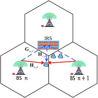
Figure 1: An IRS-aided JP-CoMP transmission multicell system.

II System Model And Problem Formulation

II-A System Model

Consider an IRS-aided JP-CoMP downlink transmission network, which consists of $N$ BSs, $K$ cell-edge users, and one IRS as shown in Fig. 1. We assume that each BS is equipped with $N_{t}>1$ transmit antennas, each cell-edge user is equipped with $N_{r}>1$ receiver antennas, and the IRS has $M$ reflecting elements. Denote the sets of BSs, users, and reflecting elements as $\cal N$, $\cal K$, and $\cal M$, respectively. We assume that the size of the considered overall area is small so that the delay between two paths are very small and can be neglected [42, 43]. Let ${\bf{H}}_{n,k}\in{{\mathbb{C}}^{N_{r}\times N_{t}}}$, ${\bf G}_{n,r}\in{{\mathbb{C}}^{M\times{N_{t}}}}$, and ${\bf H}_{r,k}\in{{\mathbb{C}}^{N_{r}\times M}}$, respectively, denote the complex equivalent baseband channel matrix between the $k$-th user and BS $n$, between BS $n$ and the IRS, and between the IRS and the $k$-th user, $\forall k\in{\cal K}$, $\forall n\in{\cal N}$.

Mathematically, the transmitted signals by BS $n$, $n\in\left\{{1,\ldots,N}\right\}$, is given by

$${{\bf{x}}_{n}}=\sum\limits_{k=1}^{K}{{{\bf{W}}_{n,k}}{{\bf{s}}_{k}}},$$ (1)

where ${{\bf{s}}_{k}}\in{{\mathbb{C}}^{d\times 1}}$ represents $d$ desired data streams for user $k$ satisfying ${{\bf{s}}_{k}}\sim{\cal CN}\left({{\bf{0}},{{\bf{I}}_{d}}}\right)$, ${{\bf{W}}_{n,k}}\in{{\mathbb{C}}^{{N_{t}}\times d}}$ stands for the transmit beamforming matrix for user $k$ by BS $n$. Note that the channel acquisition techniques for the cascaded BS-IRS-user links in the IRS-aided system cannot be applied to our scenario due to the separate CSI links are required[26, 27, 28]. To acquire the accurate CSI for the independent links such as BS-user links, IRS-BS links and IRS-user links, we assume that the IRS is equipped with some RF chains [9]. As a result, the conventional channel estimation methods for the multicell MIMO networks can be directly applied for the IRS to estimate the channels of the BS-IRS and IRS-user links. As such, we assume that the CSI for all the channel links are perfectly known by the central processor. As shown in Fig. 1, each user receives not only the desired signals from the $N$ BSs, but also the reflected signals by the IRS. Note that different from CS/CB-CoMP multicell systems, where each user data is only available at one serving BS, each user data in JP-CoMP multicell systems is available at all BSs. The received signal at user $k$ is thus given by

$${{\bf{y}}_{k}} =\;\underbrace{\sum\limits_{n=1}^{N}{{{\bf{H}}_{n,k}}{{\bf{x}}_{n}}}}_{{\rm{direct}}{\kern 1.0pt}{\kern 1.0pt}{\kern 1.0pt}{\rm{links}}}+\underbrace{{{\bf{H}}_{r,k}}{\bf{\Phi}}\sum\limits_{n=1}^{N}{{{\bf{G}}_{n,r}}{{\bf{x}}_{n}}}}_{{\rm{reflected{\kern 1.0pt}{\kern 1.0pt}{\kern 1.0pt}links}}}+{{\bf{n}}_{k}}$$

$$=\underbrace{\sum\limits_{n=1}^{N}{\left({{{\bf{H}}_{n,k}}+{{\bf{H}}_{r,k}}{\bf{\Phi}}{{\bf{G}}_{n,r}}}\right){{\bf{W}}_{n,k}}{{\bf{s}}_{k}}}}_{{\rm{desired}}{\kern 1.0pt}{\kern 1.0pt}{\rm{signals}}}+$$

$$~{}\underbrace{\sum\limits_{n=1}^{N}{\sum\limits_{j\neq k}^{K}{\left({{{\bf{H}}_{n,k}}+{{\bf{H}}_{r,k}}{\bf{\Phi}}{{\bf{G}}_{n,r}}}\right){{\bf{W}}_{n,j}}{{\bf{s}}_{j}}}}}_{{\mathop{\rm int}}{\rm{erference~{}signals}}}+{{\bf{n}}_{k}},$$ (2)

where ${\bf{\Phi}}={\rm{diag}}\left({{a_{1}e^{j{\theta_{1}}}},\cdots,{a_{M}e^{j{\theta_{M}}}}}\right)$ represents the phase shift matrix adopted at the IRS [34, 9, 31, 20, 44], where ${a_{m}}\in\left[{0,1}\right]$ and ${\theta_{m}}\in\left[{0,2\pi}\right)$ (since ${\theta_{m}}$ are periodic with respect to $2\pi$, thus we consider them in $\left[{0,2\pi}\right]$ for convenience), respectively, denote the amplitude reflection coefficient and phase shift of the $m$-th reflecting element, ${{\bf{n}}_{k}}\sim{\cal CN}\left({{\bf{0}},{\sigma^{2}}{{\bf{I}}_{{N_{r}}}}}\right)$ is the received noise with $\sigma^{2}$ denoting the noise power at each antenna. For the sake of low implementation complexity, in this paper, each element of the IRS is designed to maximize the signal reflection, i.e., $a_{m}=1$, $\forall m$.

For notational simplicity, we define ${{{\bf{\bar{H}}}}_{n,k}}={{\bf{H}}_{n,k}}+{{\bf{H}}_{r,k}}{\bf{\Phi}}{{\bf{G}}_{n,r}}$, ${{{\bf{\bar{H}}}}_{k}}=\left[{{{{\bf{\bar{H}}}}_{1,k}},\cdots,{{{\bf{\bar{H}}}}_{N,k}}}\right]$, and ${{\bf{W}}_{k}}={\left[{{\bf{W}}_{1,k}^{T},\cdots,{\bf{W}}_{N,k}^{T}}\right]^{T}}$. Then, we can rewrite (2) as

$${{\bf{y}}_{k}}={{{\bf{\bar{H}}}}_{k}}{{\bf{W}}_{k}}{{\bf{s}}_{k}}+{{{\bf{\bar{H}}}}_{k}}\sum\limits_{j\neq k}^{K}{{{\bf{W}}_{j}}{{\bf{s}}_{j}}}+{{\bf{n}}_{k}}.$$ (3)

As such, the achievable data rate (nat/s/Hz) of user $k$ is given by

$${R_{k}}=\ln\left|{{\bf{I}}_{N_{r}}+{{{\bf{\bar{H}}}}_{k}}{{\bf{W}}_{k}}{\bf{W}}_{k}^{H}{\bf{\bar{H}}}_{k}^{H}{\bf{F}}_{k}^{-1}}\right|,$$ (4)

where ${{\bf{F}}_{k}}={{{\bf{\bar{H}}}}_{k}}\left({\sum\limits_{j\neq k}^{K}{{{\bf{W}}_{j}}{\bf{W}}_{j}^{H}}}\right){\bf{\bar{H}}}_{k}^{H}+{\sigma^{2}}{\bf{I}}_{N_{r}}$.

II-B Problem Formulation

In this paper, to guarantee the user fairness, we aim at maximizing the minimum achievable rate of the users by jointly optimizing the downlink transmit beamforming and the IRS phase shift matrix, subject to transmit power constraints at the BSs. Accordingly, the problem can be formulated as

$$\left({\rm{P}}\right): \mathop{\rm maximize}\limits_{{{\bf{W}}_{n,k}},{\bm{\Phi}},R}{\kern 1.0pt}{\kern 1.0pt}{\kern 1.0pt}{\kern 1.0pt}R$$

$${\rm{s}}{\rm{.t}}{\rm{.}}{\kern 1.0pt}{\kern 1.0pt}{\kern 1.0pt}{\kern 1.0pt}{\kern 1.0pt}{\kern 1.0pt}\ln\left|{{\bf{I}}_{N_{r}}+{{{\bf{\bar{H}}}}_{k}}{{\bf{W}}_{k}}{\bf{W}}_{k}^{H}{\bf{\bar{H}}}_{k}^{H}{\bf{F}}_{k}^{-1}}\right|\geq R,{\kern 1.0pt}{\kern 1.0pt}k\in\cal K,$$ (5)

$$\qquad\sum\limits_{k=1}^{K}{\left\|{{{\bf{W}}_{n,k}}}\right\|_{F}^{2}}\leq{P_{\max}},{\kern 1.0pt}{\kern 1.0pt}n\in\cal N,$$ (6)

$$\qquad 0\leq{\theta_{m}}\leq 2\pi,{\kern 1.0pt}{\kern 1.0pt}m\in\cal M,$$ (7)

where $P_{\rm max}$ denotes the maximum BS transmit power. Although constraint (6) is convex and (7) is linear with respect to $\theta_{m}$, it is challenging to solve problem $(\rm P)$ due to the coupled transmit beamforming matrix and the phase shift matrix in (5). In general, there is no efficient method to solve problem $(\rm P)$ optimally. To facilitate the solution development, we first transform problem $(\rm P)$ into an equivalent form denoted by $(\rm P1)$ based on the mean-square error (MSE) method [47]. Specifically, the achievable rate in (4) can be viewed as a data rate for a hypothetical communication system where user $k$ estimates the desired signal ${\bf s}_{k}$ with an estimator ${{\bf{U}}_{k}}\in{{\mathbb{C}}^{{N_{r}}\times d}}$, the estimated signal is given by

$${{{\bf{\hat{s}}}}_{k}}={\bf{U}}_{k}^{H}{{\bf{y}}_{k}}.$$ (8)

As such, the MSE matrix is given by

$${{\bf{E}}_{k}}= {\mathbb{E}}\left\{{\left({{{{\bf{\hat{s}}}}_{k}}-{{\bf{s}}_{k}}}\right){{\left({{{{\bf{\hat{s}}}}_{k}}-{{\bf{s}}_{k}}}\right)}^{H}}}\right\}$$

$$= {\bf{U}}_{k}^{H}\left({{{{\bf{\bar{H}}}}_{k}}\left({\sum\limits_{j=1}^{K}{{{\bf{W}}_{j}}{\bf{W}}_{j}^{H}}}\right){\bf{\bar{H}}}_{k}^{H}+{\sigma^{2}}{\bf{I}}_{N_{r}}}\right){{\bf{U}}_{k}}$$

$$-{\bf{U}}_{k}^{H}{{{\bf{\bar{H}}}}_{k}}{{\bf{W}}_{k}}-{\bf{W}}_{k}^{H}{\bf{\bar{H}}}_{k}^{H}{{\bf{U}}_{k}}+{\bf{I}}_{d}.$$ (9)

By introducing additional variables ${{\bf{Q}}_{k}}\in{{\mathbb{C}}^{d\times d}}$ and ${{\bf{U}}_{k}}\in{{\mathbb{C}}^{{N_{r}}\times d}}$, $\forall k$, we then have the following theorem:

Theorem 1: Problem $(\rm P)$ is equivalent to $(\rm P1)$, which is shown as below:

$$\left({\rm{P1}}\right): \mathop{\rm maximize}\limits_{{{\bf{W}}_{n,k}},{\bm{\Phi}},R,{{\bf{U}}_{k}},{{\bf{Q}}_{k}}}{\kern 1.0pt}{\kern 1.0pt}{\kern 1.0pt}{\kern 1.0pt}R$$

$${\rm s.t.}~{}\ln\left|{{{\bf{Q}}_{k}}}\right|-{\rm{Tr}}\left({{{\bf{Q}}_{k}}{{\bf{E}}_{k}}}\right)+d\geq R,{\kern 1.0pt}{\kern 1.0pt}k\in\cal K,$$ (10)

$$\qquad{{\bf{Q}}_{k}}\succeq{\bf{0}},{\kern 1.0pt}{\kern 1.0pt}k\in\cal K,$$ (11)

$$\qquad\eqref{Pconst2},\eqref{Pconst3}.$$ (12)

Proof: Please refer to Appendix A.

Although $(\rm P1)$ introduces additional variables ${{\bf{Q}}_{k}}$ and ${{\bf{U}}_{k}}$, the new problem structure facilitates the design of a computationally efficient suboptimal algorithm. In the following, we first consider a single cell-edge user system, where the transmit beamforming matrix and phase shift matrix are obtained based on the dual subgradient method and majorization-minimization method, respectively. Then, we consider the joint IRS phase shift and transmit beamforming optimization problem in the multiuser system which is then handled by applying the SOCP and SDR techniques, respectively.

III Single Cell-edge User System

In this section, we consider a single cell-edge user system, namely $K=1$. For notational simplicity, we drop user index $k$ in this section. Then, the problem for the single-user system can be simplified as

$$\left({{\rm{P2}}}\right): \mathop{\rm maximize}\limits_{{{\bf{W}}_{n}},{\bm{\Phi}},{\bf{U}},{\bf{Q}}}{\kern 1.0pt}{\kern 1.0pt}{\kern 1.0pt}{\kern 1.0pt}\ln\left|{{{\bf{Q}}}}\right|-{\rm{Tr}}\left({{{\bf{Q}}}{{\bf{E}}}}\right)+d$$

$${\rm{s}}{\rm{.t}}{\rm{.}}{\kern 1.0pt}{\kern 1.0pt}{\kern 1.0pt}{\kern 1.0pt}{\kern 1.0pt}\left\|{{{\bf{W}}_{n}}}\right\|_{F}^{2}\leq{P_{\max}},{\kern 1.0pt}{\kern 1.0pt}{\kern 1.0pt}n\in\cal N,$$ (13)

$$\qquad{{\bf{Q}}}\succeq{\bf{0}},~{}\eqref{Pconst3}.$$ (14)

Although simplified, $(\rm P2)$ is still difficult to handle due to the coupled optimization variables in the objective function of $(\rm P2)$. However, we observe that both $\bf Q$ and $\bf U$ are concave with respect to the objective function of $(\rm P2)$. In addition, variable $\bf U$ does not exist in the constraint set and the variable $\bf Q$ only appears in constraint (14).

By applying the standard convex optimization technique, setting the first-order derivative of the objective function of $(\rm P2)$ with respective to $\bf U$ and $\bf Q$ to zero, the optimal solutions of $\bf U$ and $\bf Q$ can be respectively obtained as

$${{\bf{U}}^{\rm opt}}={\left({{\bf{\bar{H}WW}}{{{\bf{\bar{H}}}}^{H}}+{\sigma^{2}}{\bf{I}}_{N_{r}}}\right)^{-1}}{\bf{\bar{H}W}},$$ (15)

and

$${{\bf{Q}}^{\rm opt}}={{\bf{E}}^{-1}}.$$ (16)

To address the coupled transmit beamforming matrix and phase shift matrix, we first decouple $(\rm P2)$ into two sub-problems, namely transmit beamforming optimization with the fixed phase shift matrix and phase shift matrix optimization with the fixed transmit beamforming matrix, and then an iterative method is proposed based on the alternating optimization [47].

III-A Transmit Beamforming Matrix Optimization with Fixed Phase Shift Matrix

We first consider the first sub-problem of $(\rm P2)$, denoted as $({\rm P2}{\rm-1})$, for optimizing the BS transmit beamforming matrix ${\bf W}_{n}$ by assuming that the IRS phase shift matrix $\bm{\Phi}$ is fixed. By dropping the irrelevant constant term ${\rm ln}\left|{\bf{Q}}\right|+d-{\sigma^{2}}{\rm{Tr}}\left({{\bf{Q}}{{\bf{U}}^{H}}{\bf{U}}}\right)-{\rm{Tr}}\left({\bf{Q}}\right)$, the transmit beamforming matrix optimization problem can be simplified as

$$\left({{\rm{P2}}{\rm-1}}\right):\mathop{\rm minimize}\limits_{{{\bf{W}}_{n}}}{\kern 1.0pt}{\kern 1.0pt}{\kern 1.0pt}{\kern 1.0pt}{\rm{Tr}}\left({{\bf{Q}}{{\bf{U}}^{H}}{\bf{\bar{H}W}}{{\bf{W}}^{H}}{{{\bf{\bar{H}}}}^{H}}{\bf{U}}}\right)$$

$$\qquad\qquad-{\rm{Tr}}\left({{\bf{Q}}{{\bf{U}}^{H}}{\bf{\bar{H}W}}}\right)-{\rm{Tr}}\left({{\bf{Q}}{{\bf{W}}^{H}}{{{\bf{\bar{H}}}}^{H}}{\bf{U}}}\right)$$

$$\qquad{\rm s.t.}~{}\eqref{P2const1}.$$ (17)

Problem $({\rm P2}{\rm-1})$ is a standard convex optimization problem which can be solved by the convex tools such as CVX [48]. Instead of relying on the generic solver with high computational complexity, we propose an efficient approach based on the Lagrangian dual subgradient method. Note that it can be readily checked that problem $({\rm P2}{\rm-1})$ satisfies the Slater’s condition, thus, strong duality holds and its optimal solution can be obtained via solving its dual problem [49]. In the following, we solve $({\rm P2}{\rm-1})$ by solving its dual problem. Specifically, by introducing dual variable $\mu_{n}\geq 0,n\in\cal N$, corresponding to constraint (13), we have the Lagrangian function of $({\rm P2}{\rm-1})$ given by

$${\cal L}\left({{{\bf{W}}_{n}},{\mu_{n}}}\right)={\rm{Tr}}\left({\left({\sum\limits_{n=1}^{N}{\sum\limits_{j=1}^{N}{{{{\bf{\bar{H}}}}_{j}}{{\bf{W}}_{j}}{\bf{W}}_{n}^{H}{\bf{\bar{H}}}_{n}^{H}}}}\right){\bf{UQ}}{{\bf{U}}^{H}}}\right)-$$

$$\sum\limits_{n=1}^{N}{{\rm{Tr}}\left({{\bf{Q}}{{\bf{U}}^{H}}{{{\bf{\bar{H}}}}_{n}}{{\bf{W}}_{n}}}\right)}-\sum\limits_{n=1}^{N}{{\rm{Tr}}\left({{\bf{QW}}_{n}^{H}{\bf{\bar{H}}}_{n}^{H}{\bf{U}}}\right)}$$

$$+\sum\limits_{n=1}^{N}{{\mu_{n}}}\left({\left\|{{{\bf{W}}_{n}}}\right\|_{F}^{2}-{P_{\max}}}\right).$$ (18)

Accordingly, the dual function of $({\rm P2}{\rm-1})$ is given by

$$g\left({{\mu_{n}}}\right)=\mathop{\rm minimize}\limits_{{{\bf{W}}_{n}}}{\cal L}\left({{{\bf{W}}_{n}},{\mu_{n}}}\right).$$ (19)

Setting the first-order derivative of ${\cal L}\left({{{\bf{W}}_{n}},{\mu_{n}}}\right)$ with respect to ${{{\bf{W}}_{n}}}$ to zero yields

$${\bf{\bar{H}}}_{n}^{H}{\bf{UQ}}{{\bf{U}}^{H}}\sum\limits_{j=1}^{N}{{{{\bf{\bar{H}}}}_{j}}{{\bf{W}}_{j}}+}{\mu_{n}}{{\bf{W}}_{n}}={\bf{\bar{H}}}_{n}^{H}{\bf{UQ}},\forall n.$$ (20)

By collecting and stacking above $N$ equations, the optimal transmit beamforming matrix can be obtained as

$${{\bf{W}}^{\rm opt}}\left({{\mu_{n}}}\right)={\bf{\hat{J}}}_{1}^{-1}{{{\bf{\hat{J}}}}_{2}},$$ (21)

where ${{{\bf{\hat{J}}}}_{1}}$ is given by

$${{{\bf{\hat{J}}}}_{1}}=\left(\begin{array}[]{ccc}{\bf{\bar{H}}}_{1}^{H}{\bf{UQ}}{{\bf{U}}^{H}}{{{\bf{\bar{H}}}}_{1}}+{\mu_{1}}{\bf{I}}_{N_{t}}&\cdots&{\bf{\bar{H}}}_{1}^{H}{\bf{UQ}}{{\bf{U}}^{H}}{{{\bf{\bar{H}}}}_{N}}\\ \vdots&\cdots&\vdots\\ {\bf{\bar{H}}}_{N}^{H}{\bf{UQ}}{{\bf{U}}^{H}}{{{\bf{\bar{H}}}}_{1}}&\cdots&{\bf{\bar{H}}}_{N}^{H}{\bf{UQ}}{{\bf{U}}^{H}}{{{\bf{\bar{H}}}}_{N}}+{\mu_{N}}{\bf{I}}_{N_{t}}\\ \end{array}\right),$$ (25)

and ${{{\bf{\hat{J}}}}_{2}}$ is given by

$${{\bf{\hat{J}}}_{2}}={\left({{{\left({{\bf{H}}_{1}^{H}{\bf{UQ}}}\right)}^{T}},\cdots,{{\left({{\bf{H}}_{N}^{H}{\bf{UQ}}}\right)}^{T}}}\right)^{T}}.$$ (26)

Next, we address the corresponding dual problem, which is given by

$$\left({{\rm{P2}}}{\rm-1}{\rm D}\right):\mathop{\rm maximize}\limits_{{\mu_{n}}\geq 0}g\left({{\mu_{n}}}\right).$$ (27)

It can be seen that the dual problem $\left({{\rm{P2}}}{\rm-1}{\rm D}\right)$ has no additional constraints. In addition, with any fixed dual variable $\mu_{n}$, the optimal transmit beamforming matrix can be directly solved in a closed-form as in (21). As such, we propose an efficient method, namely subgradient method, to solve the dual problem $\left({{\rm{P2}}}{\rm-1}{\rm D}\right)$. The update rule of parameters $\{\mu_{n}\}$ is given by

$$\mu_{n}^{t+1}=\left[{\mu_{n}^{t}+{\pi_{n}}\left({\left\|{{\bf{W}}_{n}^{\rm opt}\left({u_{n}^{t}}\right)}\right\|_{F}^{2}-{P_{\max}}}\right)}\right]^{+},\forall n,$$ (28)

where superscript $t$ denotes the iteration index and ${\pi_{n}}$ represents the positive step size for updating $\mu_{n}$. The detailed descriptions of the dual subgradient method are summarized in Algorithm 1.

Algorithm 1 Subgradient Method for $\left({{\rm{P2}}}{\rm-1}\right)$.

1:  Initialize $\{\mu^{t}_{n}\}\geq 0$, $\pi_{n}\geq 0$, iteration index $t=0$.

2:  repeat

3:    Calculate the optimal transmit beamforming matrix using (21).

4:    Compute dual variable $\{\mu_{n}^{t+1}\}$ using (28).

5:    Set $t=t+1$.

6:  until the fractional increase of $\left({{\rm{P2}}}{\rm-1}{\rm D}\right)$ is smaller than a predefined threshold.

7:  Output: ${{\bf{W}}_{n}^{\rm opt}}$, $\forall n\in\left\{{1,\ldots,N}\right\}$.

III-B Phase Shift Matrix Optimization with Fixed Transmit Beamforming

Next, we consider the second sub-problem of $(\rm P2)$, denoted as $({\rm P2}{\rm-2})$, for optimizing the phase shift matrix, $\bm{\Phi}$, by assuming that the transmit beamforming matrix, ${\bf W}_{n}$, is fixed. By dropping the constant term ${\rm ln}\left|{\bf{Q}}\right|+d-{\sigma^{2}}{\rm{Tr}}\left({{\bf{Q}}{{\bf{U}}^{H}}{\bf{U}}}\right)-{\rm{Tr}}\left({\bf{Q}}\right)$, the phase shift matrix optimization problem can be simplified as

$$\left({{\rm{P2}}{\rm-2}}\right):\mathop{\rm minimize}\limits_{{\bm{\Phi}}}{\kern 1.0pt}{\kern 1.0pt}{\kern 1.0pt}{\kern 1.0pt}{\rm{Tr}}\left({{\bf{Q}}{{\bf{U}}^{H}}{\bf{\bar{H}W}}{{\bf{W}}^{H}}{{{\bf{\bar{H}}}}^{H}}{\bf{U}}}\right)-$$

$$\qquad\qquad{\rm{Tr}}\left({{\bf{Q}}{{\bf{U}}^{H}}{\bf{\bar{H}W}}}\right)-{\rm{Tr}}\left({{\bf{Q}}{{\bf{W}}^{H}}{{{\bf{\bar{H}}}}^{H}}{\bf{U}}}\right)$$

$$\qquad\qquad{\rm s.t.}~{}\eqref{Pconst3}.$$ (29)

Problem $\left({{\rm{P2}}}{\rm-2}\right)$ is a non-convex optimization problem due to the non-convex objective function. To address this issue, by expanding $\bf W$ and $\bf{\bar{H}}$, we have

$${\rm{Tr}}\left({{\bf{Q}}{{\bf{U}}^{H}}{\bf{\bar{H}W}}{{\bf{W}}^{H}}{{{\bf{\bar{H}}}}^{H}}{\bf{U}}}\right) ={\rm{Tr}}\left({{{\bf{\Phi}}^{H}}{\bf{A\Phi\tilde{E}}}}\right)+{\rm{Tr}}\left({{\bf{\Phi}}{{\bf{D}}^{H}}}\right)$$

$$+{\rm{Tr}}\left({{{\bf{\Phi}}^{H}}{\bf{D}}}\right)+{c_{2}},$$ (30)

where ${\bf{A}}={\bf{H}}_{r}^{H}{\bf{UQ}}{{\bf{U}}^{H}}{{\bf{H}}_{r}}$, ${\bf{\tilde{E}}}=\left({\sum\limits_{n=1}^{N}{{{\bf{G}}_{n,r}}{{\bf{W}}_{n}}}}\right){\left({\sum\limits_{n=1}^{N}{{{\bf{G}}_{n,r}}{{\bf{W}}_{n}}}}\right)^{H}}$, ${\bf{D}}={\bf{H}}_{r}^{H}{\bf{UQ}}{{\bf{U}}^{H}}\left({\sum\limits_{n=1}^{N}{{{\bf{H}}_{n}}{{\bf{W}}_{n}}}}\right)$ ${\left({\sum\limits_{n=1}^{N}{{{\bf{G}}_{n,r}}{{\bf{W}}_{n}}}}\right)^{H}}$, and ${c_{2}}={\rm{Tr}}\left({\left({\sum\limits_{n=1}^{N}{{{\bf{H}}_{n}}{{\bf{W}}_{n}}}}\right){{\left({\sum\limits_{n=1}^{N}{{{\bf{H}}_{n}}{{\bf{W}}_{n}}}}\right)}^{H}}{\bf{UQ}}{{\bf{U}}^{H}}}\right)$.

Similarly, we have

$${\rm{Tr}}\left({{\bf{Q}}{{\bf{W}}^{H}}{{{\bf{\bar{H}}}}^{H}}{\bf{U}}}\right)={\rm{Tr}}\left({{{\bf{\Phi}}^{H}}{\bf{B}}}\right)+{c_{1}},$$ (31)

where ${\bf{B}}={\bf{H}}_{r}^{H}{\bf{UQ}}{\left({\sum\limits_{n=1}^{N}{{{\bf{G}}_{n,r}}{{\bf{W}}_{n}}}}\right)^{H}}$ and ${c_{1}}={\rm{Tr}}\left({{\bf{Q}}{{\left({\sum\limits_{n=1}^{N}{{{\bf{H}}_{n}}{{\bf{W}}_{n}}}}\right)}^{H}}{\bf{U}}}\right)$. As such, we can equivalently transform the objective function of $\left({{\rm{P2}}}{\rm-2}\right)$ as (by dropping constants $c_{1}$ and $c_{2}$)

$$f\left({\bf{\Phi}}\right){\rm{=Tr}} \left({{{\bf{\Phi}}^{H}}{\bf{A\Phi\tilde{E}}}}\right)+{\rm{Tr}}\left({{\bf{\Phi}}{{\left({{\bf{D}}-{\bf{B}}}\right)}^{H}}}\right)+$$

$${\rm{Tr}}\left({{{\bf{\Phi}}^{H}}\left({{\bf{D}}-{\bf{B}}}\right)}\right).$$ (32)

Define ${\bm{\phi}}=\left[{{\phi_{1}},\cdots,{\phi_{M}}}\right]^{T}$, where ${\phi_{m}}={e^{j{\theta_{m}}}},m\in\cal M$, and ${\bf{z}}={\left[{{{\left[{{\bf{D}}-{\bf{B}}}\right]}_{1,1}},\cdots,{{\left[{{\bf{D}}-{\bf{B}}}\right]}_{M,M}}}\right]^{T}}$. Additionally, we have the following identities [50]

$${\rm{Tr}}\left({{{\bf{\Phi}}^{H}}{\bf{A\Phi\tilde{E}}}}\right)={{\bm{\phi}}^{H}}\left({{\bf{A}}\odot{{{\bf{\tilde{E}}}}^{T}}}\right){\bm{\phi}},$$

$${\rm{Tr}}\left({{\bf{\Phi}}{{\left({{\bf{D}}-{\bf{B}}}\right)}^{H}}}\right)={{\bf{z}}^{H}}{\bm{\phi}}.$$ (33)

Then, we can rewrite $f\left({\bm{\Phi}}\right)$ in (32) as

$$f\left({\bm{\phi}}\right)={{\bm{\phi}}^{H}}\left({{\bf{A}}\odot{{{\bf{\tilde{E}}}}^{T}}}\right){\bm{\phi}}+{{\bf{z}}^{H}}{\bm{\phi}}+{{\bm{\phi}}^{H}}{\bf{z}}.$$ (34)

As a result, problem $\left({{\rm{P2}}}{\rm-2}\right)$ is equivalent to

$$\left({{\rm{P2}}{\rm-3}}\right): \mathop{\rm minimize}\limits_{{\phi_{m}}}f\left(\bm{\phi}\right)$$

$${\rm s.t.}~{}\left|{{\phi_{m}}}\right|=1,~{}m\in\cal M.$$ (35)

Problem $\left({{\rm{P2}}}{\rm-3}\right)$ is non-convex due to the unit-modulus constraints in (35). Here, we handle $\left({{\rm{P2}}}{\rm-3}\right)$ based on the MM method, which guarantees at least a locally optimal solution with a low computational complexity [20],[51],[52]. The key idea of using the MM algorithm lies in constructing a sequence of convex surrogate functions. Specifically, at the $r$-th iteration, we need to construct an upper bound function of $f\left({\bm{\phi}}\right)$, denoted as $\hat{g}\left({\bm{\phi}|{\bm{\phi}^{r}}}\right)$, that satisfies the following three properties [51],[52]: (a) $\hat{g}\left({\bm{\phi}|{\bm{\phi}^{r}}}\right)\geq f\left(\bm{\phi}\right)$; (b) $\hat{g}\left({{\bm{\phi}^{r}}|{\bm{\phi}^{r}}}\right)=f\left({{\bm{\phi}^{r}}}\right)$; (c) ${\nabla_{{\bm{\phi}^{r}}}}\hat{g}\left({{\bm{\phi}^{r}}|{\bm{\phi}^{r}}}\right)={\nabla_{{\bm{\phi}^{r}}}}\left({{\bm{\phi}^{r}}}\right)$, where (a) denotes that $\hat{g}\left({\bm{\phi}|{\bm{\phi}^{r}}}\right)$ is an upper-bounded function of $f\left({\bm{\phi}}\right)$, (b) represents that $\hat{g}\left({\bm{\phi}|{\bm{\phi}^{r}}}\right)$ and $f\left({\bm{\phi}}\right)$ have the same solutions at point ${{\bm{\phi}^{r}}}$, and (c) indicates $\hat{g}\left({\bm{\phi}|{\bm{\phi}^{r}}}\right)$ and $f\left({\bm{\phi}}\right)$ have the same gradient at point ${{\bm{\phi}^{r}}}$.

Note that in (34), we can see that $\bf A$ and ${\bf{\tilde{E}}}$ are semidefinite matrices, and it can be readily checked that $\left({{\bf{A}}\odot{{{\bf{\tilde{E}}}}^{T}}}\right)$ is also a semidefinite matrix. In the sequence, we have the following lemma:

Lemma 1: Based on [52], at the $r$-th iteration, the surrogate function $\hat{g}\left({\bm{\phi}|{\bm{\phi}^{r}}}\right)$ for a quadratic function can be expressed as

$$\hat{g}\left({\bm{\phi}|{\bm{\phi}^{r}}}\right)={\lambda_{\max}}{\bm{\phi}^{H}}\bm{\phi}-2{\mathop{\rm Re}\nolimits}\left\{{{\bm{\phi}^{H}}\left({{\lambda_{\max}}{\bf{I}}_{M}-{\bf{A}}\odot{{{\bf{\tilde{E}}}}^{T}}}\right){\bm{\phi}^{r}}}\right\}$$

$$+{\left({{\bm{\phi}^{r}}}\right)^{H}}\left({{\lambda_{\max}}{\bf{I}}_{M}-{\bf{A}}\odot{{{\bf{\tilde{E}}}}^{T}}}\right){\bm{\phi}^{r}}+{{\bf{z}}^{H}}\bm{\phi}+{\bm{\phi}^{H}}{\bf{z}},$$ (36)

where ${\lambda_{\max}}$ is the maximum eigenvalue of ${{\bf{A}}\odot{{{\bf{\tilde{E}}}}^{T}}}$. Therefore, at any $r$-th iteration, we solve the following problem

$$\left({{\rm{P2}}{\rm-4}}\right): \mathop{\rm minimize}\limits_{{\bm{\phi}_{m}}}\hat{g}\left({\bm{\phi}|{\bm{\phi}^{r}}}\right)$$

$${\rm s.t.}~{}\left|{{\phi_{m}}}\right|=1,~{}m\in\cal M.$$ (37)

Since ${\bm{\phi}^{H}}\bm{\phi}=M$, at the $r$-th iteration, we can rewrite $\hat{g}\left({\bm{\phi}|{\bm{\phi}^{r}}}\right)$ as

$$\hat{g}\left({\bm{\phi}|{\bm{\phi}^{r}}}\right)={\lambda_{\max}}M+2{\mathop{\rm Re}\nolimits}\left\{{{\bm{\phi}^{H}}{{\bf{q}}^{r}}}\right\},$$ (38)

where ${{\bf{q}}^{r}}=\left({{\bf{z}}-\left({{\lambda_{\max}}{\bf{I}}_{M}-{\bf{A}}\odot{{{\bf{\tilde{E}}}}^{T}}}\right){\bm{\phi}^{r}}}\right)$. Obviously, the optimal solution $\bm{\phi}$ to minimize problem $\left({{\rm{P2}}}{\rm-4}\right)$ is given by

$${{\bm{\phi}}^{r,\rm opt}}={e^{-j\arg\left({{{\bf{q}}^{r}}}\right)}}.$$ (39)

The details of the proposed MM method are summarized in Algorithm 2.

Algorithm 2 MM Algorithm for $\left({{\rm{P2}}}{\rm-2}\right)$.

1:  Initialize ${\bm{\phi}^{r}}$, and set iteration index $r=0$.

2:    Compute the maximum eigenvalue of ${{\bf{A}}\odot{{{\bf{\tilde{E}}}}^{T}}}$, denoted as ${\lambda_{\max}}$.

3:  repeat

4:    Calculate ${{\bf{q}}^{r}}=\left({{\bf{z}}-\left({{\lambda_{\max}}{\bf{I}}_{M}-{\bf{A}}\odot{{{\bf{\tilde{E}}}}^{T}}}\right){\bm{\phi}^{r}}}\right)$.

5:    Obtain the optimal phase shift ${\bm{\phi}^{r,\rm opt}}$ using (39).

6:    ${\bm{\phi}^{r+1}}={\bm{\phi}^{r,\rm opt}}$.

7:    Set $r=r+1$.

8:  until the fractional decrease of $\left({{\rm{P2}}}{\rm-4}\right)$ is smaller than a threshold.

9:  Output: ${\bm{\phi}^{\rm opt}}$.

III-C Overall Algorithm

Algorithm 3 MSE-based Algorithm for $(\rm P2)$.

1:  Initialize ${\bf W}_{n}$ satisfying $\left\|{{{\bf{W}}_{n}}}\right\|_{F}^{2}={P_{\max}}$.

2:  repeat

3:    Calculate ${{\bf{U}}^{\rm opt}}$ from (15).

4:    Calculate ${{\bf{Q}}^{\rm opt}}$ from (16).

5:    Calculate ${{{\bf{W}}_{n}^{\rm opt}}}$ from Algorithm 1.

6:    Calculate ${{\bf{\Phi}}^{\rm opt}}$ from Algorithm 2.

7:  until the fractional increase of the objective value of $(\rm P2)$ is less than a predefined threshold.

Based on the solutions to two sub-problems, an efficient iterative algorithm is proposed, which is summarized in Algorithm 3. To facilitate the analysis of algorithm, we define ${{\bf{U}}^{{\rm{opt,}}r}}$, ${{\bf{Q}}^{{\rm{opt,}}r}}$, ${\bf{W}}_{n}^{{\rm{opt,}}r}$, and ${{\bf{\Phi}}^{{\rm{opt,}}r}}$ as the solution variables in the $r$-th iteration. Let $R\left({{{\bf{U}}^{{\rm{opt,}}r}},{{\bf{Q}}^{{\rm{opt,}}r}},{\bf{W}}_{n}^{{\rm{opt,}}r},{{\bf{\Phi}}^{{\rm{opt,}}r}}}\right)$ and $R_{\bf{\Phi}}^{{\rm{upper}}}\left({{{\bf{U}}^{{\rm{opt,}}r}},{{\bf{Q}}^{{\rm{opt,}}r}},{\bf{W}}_{n}^{{\rm{opt,}}r},{{\bf{\Phi}}^{{\rm{opt,}}r}}}\right)$ be the respective objective value of problems $\left({{\rm{P2}}}\right)$ and $\left({{\rm{P2}}}{\rm-4}\right)$.

In the $r$-th iteration, in step 3 of Algorithm 3, we have

$$R\left({{{\bf{U}}^{{\rm{opt}},r}},{{\bf{Q}}^{{\rm{opt}},r}},{\bf{W}}_{n}^{{\rm{opt}},r},{{\bf{\Phi}}^{{\rm{opt}},r}}}\right)$$

$$\leq R\left({{{\bf{U}}^{{\rm{opt}},r+1}},{{\bf{Q}}^{{\rm{opt}},r}},{\bf{W}}_{n}^{{\rm{opt}},r},{{\bf{\Phi}}^{{\rm{opt}},r}}}\right),$$ (40)

where the inequality holds due to the fact that $\left({{\rm{P2}}}\right)$ is optimally solved with the fixed other variables.

Similar to step 4 and step 5, we respectively have

$$R\left({{{\bf{U}}^{{\rm{opt}},r+1}},{{\bf{Q}}^{{\rm{opt}},r}},{\bf{W}}_{n}^{{\rm{opt}},r},{{\bf{\Phi}}^{{\rm{opt}},r}}}\right)$$

$$\leq R\left({{{\bf{U}}^{{\rm{opt}},r+1}},{{\bf{Q}}^{{\rm{opt}},r+1}},{\bf{W}}_{n}^{{\rm{opt}},r},{{\bf{\Phi}}^{{\rm{opt}},r}}}\right),$$ (41)

and

$$R\left({{{\bf{U}}^{{\rm{opt}},r+1}},{{\bf{Q}}^{{\rm{opt}},r+1}},{\bf{W}}_{n}^{{\rm{opt}},r},{{\bf{\Phi}}^{{\rm{opt}},r}}}\right)$$

$$\leq R\left({{{\bf{U}}^{{\rm{opt}},r+1}},{{\bf{Q}}^{{\rm{opt}},r+1}},{\bf{W}}_{n}^{{\rm{opt}},r+1},{{\bf{\Phi}}^{{\rm{opt}},r}}}\right).$$ (42)

In step 6, we have

$$R\left({{{\bf{U}}^{{\rm{opt}},r+1}},{{\bf{Q}}^{{\rm{opt}},r+1}},{\bf{W}}_{n}^{{\rm{opt}},r+1},{{\bf{\Phi}}^{{\rm{opt}},r}}}\right)$$

$$\overset{(a)}{=}-R_{\bf{\Phi}}^{{\rm{upper}}}\left({{{\bf{U}}^{{\rm{opt}},r+1}},{{\bf{Q}}^{{\rm{opt}},r+1}},{\bf{W}}_{n}^{{\rm{opt}},r+1},{{\bf{\Phi}}^{{\rm{opt}},r}}}\right)+\Upsilon$$

$$\overset{(b)}{\leq}-R_{\bf{\Phi}}^{{\rm{upper}}}\left({{{\bf{U}}^{{\rm{opt}},r+1}},{{\bf{Q}}^{{\rm{opt}},r+1}},{\bf{W}}_{n}^{{\rm{opt}},r+1},{{\bf{\Phi}}^{{\rm{opt}},r+1}}}\right)+\Upsilon$$

$$\overset{(c)}{\leq}R\left({{{\bf{U}}^{{\rm{opt}},r+1}},{{\bf{Q}}^{{\rm{opt}},r+1}},{\bf{W}}_{n}^{{\rm{opt}},r+1},{{\bf{\Phi}}^{{\rm{opt}},r+1}}}\right),$$ (43)

where $\Upsilon={\rm{ln}}\left|{\bf{Q}}\right|+d-{\sigma^{2}}{\rm{Tr}}\left({{\bf{Q}}{{\bf{U}}^{H}}{\bf{U}}}\right)-{\rm{Tr}}\left({\bf{Q}}\right)$ is a constant term irrelevant to phase shift variable ${\bf{\Phi}}$ shown in Section III-B. Note that the equality $(a)$ holds since the surrogate function $\hat{g}\left({\bm{\phi}|{\bm{\phi}^{r}}}\right)$ in (33) is tight at the given local point ${{\bm{\phi}}^{r}}$, which indicates that problem $\left({{\rm{P2}}}{\rm-3}\right)$ at ${{\bm{\phi}}^{r}}$ has the same objective value as that of problem $\left({{\rm{P2}}}{\rm-4}\right)$. Besides, inequality $(b)$ holds since problem $\left({{\rm{P2}}}{\rm-4}\right)$ is optimally solved by Algorithm 2. Also, $(c)$ is due to that the objective value of $\left({{\rm{P2}}}{\rm-4}\right)$ is served as a upper bound to that of $\left({{\rm{P2}}}{\rm-3}\right)$.

Based on (40)-(43), it yields the following inequality

$$R\left({{{\bf{U}}^{{\rm{opt}},r}},{{\bf{Q}}^{{\rm{opt}},r}},{\bf{W}}_{n}^{{\rm{opt}},r},{{\bf{\Phi}}^{{\rm{opt}},r}}}\right)$$

$$\leq R\left({{{\bf{U}}^{{\rm{opt}},r+1}},{{\bf{Q}}^{{\rm{opt}},r+1}},{\bf{W}}_{n}^{{\rm{opt}},r+1},{{\bf{\Phi}}^{{\rm{opt}},r+1}}}\right).$$ (44)

The inequality (44) shows that the objective value of $\left({{\rm{P2}}}\right)$ is non-decreasing over iterations. In addition, the maximum objective objective value of $\left({{\rm{P2}}}\right)$ is upper bounded by a finite value due to the limited BS transmit power and the finite number of IRS reflecting elements. As such, Algorithm 3 is guaranteed to converge.

The complexity analysis of Algorithm 3 is given as below. In step 3, the complexity of computing ${{\bf{U}}^{\rm opt}}$ is ${\cal O}\left({N_{r}^{3}}\right)$. In step 4, the complexity of computing ${{\bf{Q}}^{\rm opt}}$ is ${\cal O}\left({d^{3}}\right)$. In step 5, the complexity of computing ${{\bf{W}}_{n}^{\rm opt}}$ is ${\cal O}{\left({{K_{\mu}}N}\right)^{2}}$, where ${{K_{\mu}}}$ is number of iterations required for updating $\mu_{n}$ [53],[54]. In step 6, the complexity of computing the maximum eigenvalue, i.e., ${\lambda_{\max}}$, of ${{\bf{A}}\odot{{{\bf{\tilde{E}}}}^{T}}}$ is ${\cal O}\left({M^{3}}\right)$, and the complexity of computing ${{\bf{q}}^{r}}$ is ${\cal O}{\left(M^{2}\right)}$, then the total complexity of Algorithm 2 is ${\cal O}{\left({{K_{\rm mm}}M}^{2}+M^{3}\right)}$, where ${{K_{\rm mm}}}$ is the total number of iterations required by Algorithm 2 to converge. Therefore, the total complexity of Algorithm 3 is ${\cal O}\left({{K_{\rm mse}}\left({N_{r}^{3}+{d^{3}}+{{\left({{K_{\mu}}N}\right)}^{2}}+{K_{\rm mm}}{M^{2}}+{M^{3}}}\right)}\right)$, where $K_{\rm mse}$ represents the total number of iterations required by Algorithm 3 to converge.

IV Multiple Cell-Edge Users System

In this section, we consider the multiuser scenario shown in Fig. 1. To handle problem $(\rm P1)$, it can be seen in Appendix A, the optimal ${{\bf{Q}}_{k}^{\rm opt}}$ and ${\bf{U}}_{k}^{{}^{\rm opt}}$ can be directly obtained from (76) and (77), respectively. Similar to the single-user system, we decompose $(\rm P1)$ into two sub-problems, namely transmit beamforming matrix optimization with the fixed phase shift matrix and performing phase shift matrix optimization with the fixed transmit beamforming matrix. Note that the proposed MM method and the dual subgradient method in the single-user system cannot be applied to the multiuser system due to constraint (10) in $(\rm P1)$. However, in the following, we resort to SOCP technique to solve the transmit beamforming matrix optimization sub-problem, and the SDR technique to address the phase shift matrix optimization sub-problem.

IV-A SOCP for Transmit Beamforming Matrix Optimization

By fixing the phase shifts at the IRS, the transmit beamforming optimization problem is

$$\left({\rm{P1}}{\rm-1}\right): \mathop{\rm maximize}\limits_{{{\bf{W}}_{n,k}},R}{\kern 1.0pt}{\kern 1.0pt}{\kern 1.0pt}{\kern 1.0pt}R$$

$${\rm s.t.}~{}\eqref{Pconst2},\eqref{P1const1}.$$ (45)

It is not difficult to observe that $\left({\rm{P1}}{\rm-1}\right)$ is a convex optimization problem and can be transformed into a semidefinite program (SDP) problem. According to [55], the SOCP has a much lower worst-case computational complexity than that of the SDP method by applying the interior-point method to solve problem $\left({\rm{P1}}{\rm-1}\right)$. We have the following theorem:

Theorem 2: Problem $\left({\rm{P1}}{\rm-1}\right)$ is equivalent to the following SOCP problem:

$$\left({\rm{P1}}{\rm-2}\right):\mathop{\rm maximize}\limits_{{{\bf{W}}_{n,k}},R}{\kern 1.0pt}{\kern 1.0pt}{\kern 1.0pt}{\kern 1.0pt}R$$

$${\rm s.t.}~{}{\left\|{{{\bm{\eta}}_{n}}}\right\|_{2}}\leq\sqrt{{P_{\max}}},\forall n,$$ (46)

$$\qquad{\left\|{{{\bm{\omega}}_{k}}}\right\|_{2}}\leq\sqrt{\ln\left|{{{\bf{Q}}_{k}}}\right|+d-R-{\sigma^{2}}{\rm{Tr}}\left({{{\bf{Q}}_{k}}{\bf{U}}_{k}^{H}{{\bf{U}}_{k}}}\right)},\forall k,$$ (47)

where ${\left\|{{{\bm{\eta}}_{n}}}\right\|_{2}}$ and ${\left\|{{{\bm{\omega}}_{k}}}\right\|_{2}}$ are, respectively, given in (82) and (85) in Appendix B.

Proof: Please refer to Appendix B.

Therefore, $\left({\rm{P1}}{\rm-2}\right)$ is a standard SOCP problem, which can be optimally solved by the interior point method [49].

IV-B SDR Technique for Phase Shift Matrix Optimization

Next, by fixing the transmit beamforming matrix, the phase shift matrix optimization problem, denoted by $\left({\rm{P1}}{\rm-3}\right)$, can be formulated as

$$\left({\rm{P1}}{\rm-3}\right): \mathop{\rm maximize}\limits_{{\bm{\Phi}},R}{\kern 1.0pt}{\kern 1.0pt}{\kern 1.0pt}{\kern 1.0pt}R$$

$${\rm s.t.}~{}\eqref{Pconst3},\eqref{P1const1}.$$ (48)

Problem $\left({\rm{P1}}{\rm-3}\right)$ is non-convex due to the non-convex constraint (10). To tackle this non-convex problem, the SDR technique is applied. By using ${{{\bf{\bar{H}}}}_{n,k}}={{\bf{H}}_{n,k}}+{{\bf{H}}_{r,k}}{\bf{\Phi}}{{\bf{G}}_{n,r}}$ and ${{{\bf{\bar{H}}}}_{k}}=\left[{{{{\bf{\bar{H}}}}_{1,k}},\cdots,{{{\bf{\bar{H}}}}_{N,k}}}\right]$, we have

$${\rm{Tr}}\left({{{\bf{Q}}_{k}}{\bf{U}}_{k}^{H}{{{\bf{\bar{H}}}}_{k}}\left({\sum\limits_{j=1}^{K}{{{\bf{W}}_{j}}{\bf{W}}_{j}^{H}}}\right){\bf{\bar{H}}}_{k}^{H}{{\bf{U}}_{k}}}\right)$$

$$={\rm{Tr}}\left({{{\bf{\Phi}}^{H}}{{\bf{A}}_{k}}{\bf{\Phi}}{{{\bf{\check{E}}}}}}\right)+{\rm{Tr}}\left({{\bf{\Phi D}}_{k}^{H}}\right)+{\rm{Tr}}\left({{{\bf{\Phi}}^{H}}{{\bf{D}}_{k}}}\right)+{c_{k,2}},$$ (49)

and

$${\rm{Tr}}\left({{{\bf{Q}}_{k}}{\bf{W}}_{k}^{H}{\bf{\bar{H}}}_{k}^{H}{\bf{U}}_{k}^{H}}\right)={\rm{Tr}}\left({{{\bf{\Phi}}^{H}}{{\bf{B}}_{k}}}\right)+{c_{k,1}},$$ (50)

where

$${{\bf{A}}_{k}}={\bf{H}}_{r,k}^{H}{{\bf{U}}_{k}}{{\bf{Q}}_{k}}{\bf{U}}_{k}^{H}{{\bf{H}}_{r,k}},{{\bf{B}}_{k}}={\bf{H}}_{r,k}^{H}{{\bf{U}}_{k}}{{\bf{Q}}_{k}}{\bf{L}}_{1,k}^{H},$$ (51)

$$\mathop{\bf{\check{E}}}\limits=\sum\limits_{j=1}^{K}{{{{\bf{L}}_{1,j}}{\bf{L}}_{1,j}^{H}}},$$ (52)

$${{\bf{D}}_{k}}={\bf{H}}_{r,k}^{H}{{\bf{U}}_{k}}{{\bf{Q}}_{k}}{\bf{U}}_{k}^{H}\sum\limits_{j=1}^{K}{{{\bf{L}}_{2,k,j}}{\bf{L}}_{1,j}^{H}},$$ (53)

$${c_{k,1}}={\rm{Tr}}\left({{{\bf{Q}}_{k}}{\bf{L}}_{2,k,k}^{H}{{\bf{U}}_{k}}}\right),$$ (54)

$${c_{k,2}}={\rm{Tr}}\left({\sum\limits_{j=1}^{K}{{{\bf{L}}_{2,k,j}}{\bf{L}}_{2,k,j}^{H}}{{\bf{U}}_{k}}{{\bf{Q}}_{k}}{\bf{U}}_{k}^{H}}\right),$$ (55)

where ${{\bf{L}}_{1,k}}=\sum\limits_{n=1}^{N}{{{\bf{G}}_{n,r}}{{\bf{W}}_{n,k}},\forall k}$, and ${{\bf{L}}_{2,k,j}}=\sum\limits_{n=1}^{N}{{{\bf{H}}_{n,k}}{{\bf{W}}_{n,j}}},\forall k,j$.

As a result, we can rewrite $\left({\rm{P1}}{\rm-3}\right)$ as

$$\left({\rm{P1}}{\rm-4}\right):\mathop{\max}\limits_{{\bm{\Phi}},R}{\kern 1.0pt}{\kern 1.0pt}{\kern 1.0pt}{\kern 1.0pt}R$$

$${\rm s.t.}~{}{\rm{Tr}}\left({{{\bf{\Phi}}^{H}}{{\bf{A}}_{k}}{\bf{\Phi}}{{{\bf{\check{E}}}}}}\right)+{\rm{Tr}}\left({{{\bf{\Phi}}^{H}}\left({{{\bf{D}}_{k}}-{{\bf{B}}_{k}}}\right)}\right)$$

$$\quad+{\rm{Tr}}\left({{\bf{\Phi}}{{\left({{{\bf{D}}_{k}}-{{\bf{B}}_{k}}}\right)}^{H}}}\right)\leq{\rm{cons}}{{\rm{t}}_{k}}-R,\forall k,$$ (56)

$$\qquad\eqref{Pconst3},$$

where ${\rm{cons}}{{\rm{t}}_{k}}=\ln\left|{{{\bf{Q}}_{k}}}\right|+d+2{\mathop{\rm Re}\nolimits}\left({{c_{k,1}}}\right)-{c_{k,2}}-{\rm{Tr}}\left({{{\bf{Q}}_{k}}\left({{\sigma^{2}}{\bf{U}}_{k}^{H}{{\bf{U}}_{k}}+{\bf{I}}}_{d}\right)}\right)$. Similar to (34), define ${\bm{\phi}}=\left[{{\phi_{1}},\cdots,{\phi_{M}}}\right]^{T}$, where ${\phi_{m}}={e^{j{\theta_{m}}}},m\in\cal M$, and ${{\bf{z}}_{k}}={\left[{{{\left[{{{\bf{D}}_{k}}-{{\bf{B}}_{k}}}\right]}_{1,1}},\cdots,{{\left[{{{\bf{D}}_{k}}-{{\bf{B}}_{k}}}\right]}_{M,M}}}\right]^{T}},\forall k$. Based on the identities (33), we thus have ${\rm{Tr}}\left({{{\bf{\Phi}}^{H}}{{\bf{A}}_{k}}{\bm{\Phi}}{{{\bf{\check{E}}}}}}\right)={\bm{\phi}^{H}}\left({{{\bf{A}}_{k}}\odot{\bf{\check{E}}}^{T}}\right)\bm{\phi}$, ${\rm{Tr}}\left({{{\bf{\Phi}}^{H}}\left({{{\bf{D}}_{k}}-{{\bf{B}}_{k}}}\right)}\right)={\bm{\phi}^{H}}{{\bf{z}}_{k}}$, and ${\rm{Tr}}\left({{\bf{\Phi}}{{\left({{{\bf{D}}_{k}}-{{\bf{B}}_{k}}}\right)}^{H}}}\right)={\bf{z}}_{k}^{H}\bm{\phi}$. Define $\bar{\bm{\phi}}={\left[{{{\bm{\phi}}^{T}}{\kern 1.0pt}{\kern 1.0pt}{\kern 1.0pt}{\kern 1.0pt}{\kern 1.0pt}1}\right]^{T}}$. Problem $\left({\rm{P1}}{\rm-4}\right)$ is equivalent to

$$\left({\rm{P1}}{\rm-5}\right): \mathop{\rm maximize}\limits_{{\phi_{m}},R}{\kern 1.0pt}{\kern 1.0pt}{\kern 1.0pt}{\kern 1.0pt}R$$

$${\rm s.t.}~{}{{\bar{\bm{\phi}}}^{H}}{{\bm{\Psi}}_{k}}\bar{\bm{\phi}}\leq{\rm{cons}}{{\rm{t}}_{k}}-R,\forall k,$$ (57)

$$\qquad\left|{{\phi_{m}}}\right|=1,\forall m,$$ (58)

where ${{\bm{\Psi}}_{k}}=\left(\begin{array}[]{ccc}{{{\bf{A}}_{k}}\odot{\bf{\check{E}}}^{T}}&{{\bf{z}}_{k}}\\ {\bf{z}}_{k}^{H}&0\\ \end{array}\right)$. However, $\left({\rm{P1}}{\rm-5}\right)$ is still non-convex. Note that ${{\bar{\bm{\phi}}}^{H}}{{\bm{\Psi}}_{k}}\bar{\bm{\phi}}={\rm{Tr}}\left({{{\bm{\Psi}}_{k}}\bar{\bm{\phi}}{{\bar{\bm{\phi}}}^{H}}}\right)$. Define new variable ${\bf\Theta}=\bar{\bm{\phi}}{{\bar{\bm{\phi}}}^{H}}$, which satisfies ${\bf\Theta}\succeq\bf 0$ and ${\rm{rank}}\left({\bf\Theta}\right)=1$. Since the rank-one constraint is non-convex, we apply SDR to relax this constraint. The resulting problem is given by

$$\left({\rm{P1}}{\rm-6}\right): \mathop{\rm maximize}\limits_{{\bf\Theta},R}{\kern 1.0pt}{\kern 1.0pt}{\kern 1.0pt}{\kern 1.0pt}R$$

$${\rm s.t.}~{}{\rm{Tr}}\left({{{\bm{\Psi}}_{k}}{\bf{\Theta}}}\right)\leq{\rm{cons}}{{\rm{t}}_{k}}-R,\forall k,$$ (59)

$$\qquad{\bm{\Theta}}\succeq\bf 0,$$ (60)

$$\qquad{{\bf{\Theta}}_{m,m}}=1,\forall m,$$ (61)

which is a standard SDP. Therefore, $\left({\rm{P1}}{\rm-6}\right)$ can be efficiently solved by using the interior point methods [49]. However, due to the relaxation for $\left({\rm{P1}}{\rm-6}\right)$, the optimal matrix ${\bf{\Theta}}^{\rm opt}$ obtained by solving $\left({\rm{P1}}{\rm-6}\right)$ may not be rank-one in general. Thus, if the rank of ${\bf{\Theta}}^{\rm opt}$ is one, then we can obtain the optimal ${\bar{\bm{\phi}}}$ by performing singular value decomposition on ${\bf{\Theta}}^{\rm opt}$, otherwise, we need to construct a rank-one solution from the obtained ${\bf{\Theta}}^{\rm opt}$. To address this rank-one issue, we can apply three effective randomization techniques proposed in [56] to obtain a suboptimal solution, the details are omitted here for brevity.

IV-C Overall Algorithm

Based on the solutions to the above two sub-problems, an efficient iterative approach based on the alternating algorithm is proposed, which is summarized in Algorithm 4.

Algorithm 4 Alternating optimization for $(\rm P1)$.

1:  Initialize ${\bf W}^{r}_{n,k}$ satisfying $\left\|{{{\bf{W}}^{r}_{n,k}}}\right\|_{F}^{2}={{{P_{\max}}}\mathord{\left/{\vphantom{{{P_{\max}}}K}}\right.\kern-1.2pt}K}$, and $r=0$.

2:  repeat

3:   Update ${{\bf{U}}^{{\rm opt},r+1}}$ from (77).

4:   Update ${{\bf{Q}}^{{\rm opt},r+1}}$ from (76).

5:   Update ${{{\bf{W}}_{n,k}^{{\rm opt},r+1}}}$ from $\left({\rm{P1}}{\rm-2}\right)$.

6:   Update ${{\bf{\Phi}}^{{\rm opt},r+1}}$ from $\left({\rm{P1}}{\rm-6}\right)$.

7:   If the objective value of $\left({{\rm{P1}}}{\rm-6}\right)$ is smaller than that of $\left({{\rm{P1}}}{\rm-2}\right)$, we set ${{\bf{\Phi}}^{{\rm{opt}},r+1}}{\rm{=}}{{\bf{\Phi}}^{{\rm{opt}},r}}$.

8:   Set $r=r+1$.

9:  until the fractional increase of the objective value of $(\rm P1)$ is less than a threshold.

To facilitate the analysis of algorithm, we define ${{\bf{U}}^{{\rm{opt,}}r}}$, ${{\bf{Q}}^{{\rm{opt,}}r}}$, ${\bf{W}}_{n,k}^{{\rm{opt,}}r}$, and ${{\bf{\Phi}}^{{\rm{opt,}}r}}$ as the solution variables in the $r$-th iteration. Let $\bar{R}\left({{{\bf{U}}^{{\rm{opt}},r}},{{\bf{Q}}^{{\rm{opt}},r}},{\bf{W}}_{n,k}^{{\rm{opt}},r},{{\bf{\Phi}}^{{\rm{opt}},r}}}\right)$ be the objective value of problem $\left({{\rm{P1}}}\right)$. In the $r$-th iteration, from step 3 to step 5 in Algorithm 4, we have

$$\bar{R}\left({{{\bf{U}}^{{\rm{opt}},r}},{{\bf{Q}}^{{\rm{opt}},r}},{\bf{W}}_{n,k}^{{\rm{opt}},r},{{\bf{\Phi}}^{{\rm{opt}},r}}}\right)$$

$$\leq\bar{R}\left({{{\bf{U}}^{{\rm{opt}},r+1}},{{\bf{Q}}^{{\rm{opt}},r}},{\bf{W}}_{n,k}^{{\rm{opt}},r},{{\bf{\Phi}}^{{\rm{opt}},r}}}\right)$$

$$\leq\bar{R}\left({{{\bf{U}}^{{\rm{opt}},r+1}},{{\bf{Q}}^{{\rm{opt}},r+1}},{\bf{W}}_{n,k}^{{\rm{opt}},r},{{\bf{\Phi}}^{{\rm{opt}},r}}}\right)$$

$$\leq\bar{R}\left({{{\bf{U}}^{{\rm{opt}},r+1}},{{\bf{Q}}^{{\rm{opt}},r+1}},{\bf{W}}_{n,k}^{{\rm{opt}},r+1},{{\bf{\Phi}}^{{\rm{opt}},r}}}\right).$$ (62)

This inequity holds due to the fact at each step, the optimization variable is optimally solved. Note that in step 6, we handle problem $\left({{\rm{P1}}}{\rm-6}\right)$ by using SDR method with Gaussian randomization procedure to construct a rank-one solution from the obtained ${\bf{\Theta}}^{\rm opt}$, which may not result in a monotonic improvement property of Algorithm 4. To tackle this issue, one promising solution is to perform a significant number of randomization processes and select the best solution that maximizes the objective value of $\left({{\rm{P1}}}{\rm-6}\right)$. Specifically, suppose that the eigenvalue decomposition of ${\bf{\Theta}}^{\rm opt}$ is ${{\bf{\Theta}}^{{\rm{opt}}}}={\bf{U}}_{\bf{\Theta}}{\Sigma_{\bf{\Theta}}}{\bf{V}}_{\bf{\Theta}}$ and we choose ${\tilde{\bm{\phi}}}$ such that ${\tilde{\bm{\phi}}}={\bf{U}}_{\bf{\Theta}}\Sigma_{{}_{\bf{\Theta}}}^{1/2}{\bf{v}}$, where ${\bf{v}}$ is a vector of zero-mean, unit-variance complex circularly symmetric uncorrelated Gaussian random variables. We then construct a feasible solution ${{\bar{\bm{\phi}}}}$ as ${\bar{\bm{\phi}}}=\exp\left({j\arg\left({\frac{{{\tilde{\bm{\phi}}}}}{{{{\left[{{\tilde{\bm{\phi}}}}\right]}_{M+1}}}}}\right)}\right)$. In our simulation, for each iteration, we perform $1000$ random realizations for ${\bf{v}}$, and then choose the best solution ${\bar{\bm{\phi}}}$ that maximizes the objective value of $\left({{\rm{P1}}}{\rm-6}\right)$. If the objective value of $\left({{\rm{P1}}}{\rm-6}\right)$ is smaller than that of $\left({{\rm{P1}}}{\rm-2}\right)$, we set ${{\bf{\Phi}}^{{\rm{opt}},r+1}}{\rm{=}}{{\bf{\Phi}}^{{\rm{opt}},r}}$ as the same solution as the last iteration. If the objective value of $\left({{\rm{P1}}}{\rm-6}\right)$ is larger than that of $\left({{\rm{P1}}}{\rm-2}\right)$, we update variable ${\bf{\Phi}}$. As a result, we always have

$$\bar{R}\left({{{\bf{U}}^{{\rm{opt}},r+1}},{{\bf{Q}}^{{\rm{opt}},r+1}},{\bf{W}}_{n,k}^{{\rm{opt}},r+1},{{\bf{\Phi}}^{{\rm{opt}},r}}}\right)$$

$$\leq\bar{R}\left({{{\bf{U}}^{{\rm{opt}},r+1}},{{\bf{Q}}^{{\rm{opt}},r+1}},{\bf{W}}_{n,k}^{{\rm{opt}},r+1},{{\bf{\Phi}}^{{\rm{opt}},r+1}}}\right).$$ (63)

Based on (62) and (63), it yields the following inequality

$$\bar{R}\left({{{\bf{U}}^{{\rm{opt}},r}},{{\bf{Q}}^{{\rm{opt}},r+1}},{\bf{W}}_{n,k}^{{\rm{opt}},r},{{\bf{\Phi}}^{{\rm{opt}},r}}}\right)$$

$$\leq\bar{R}\left({{{\bf{U}}^{{\rm{opt}},r+1}},{{\bf{Q}}^{{\rm{opt}},r+1}},{\bf{W}}_{n,k}^{{\rm{opt}},r+1},{{\bf{\Phi}}^{{\rm{opt}},r+1}}}\right).$$ (64)

The inequality (64) shows that the objective value of $\left({{\rm{P1}}}\right)$ is non-decreasing over iterations. In addition, the maximum objective objective value of $\left({{\rm{P1}}}\right)$ is upper bounded by a finite value due to the limited BS transmit power and the finite number of IRS reflecting elements. As such, by applying the proposed Algorithm 4, the objective value is guaranteed to be non-decreasing over the iterations and terminated finally. Note that although our proposed Algorithm 4 cannot guarantee to obtain a local and/or optimal solution, it provides a feasible solution to the highly non-convex $\left({{\rm{P1}}}\right)$ with much low complexity. In addition, in Section V-B, the simulation results showed a good monotonic improvement property of Algorithm 4, which demonstrate its effectiveness.

The complexity of Algorithm 4 is given as follows: In step 3, the complexity of computing ${{\bf{U}}_{k}}$ is ${\cal O}\left({KN_{r}^{3}}\right)$. In step 4, the complexity of computing ${{\bf{Q}}_{k}}$ is ${\cal O}\left({K{d^{3}}}\right)$. In step 5, $\left({\rm{P1}}{\rm-2}\right)$ is a standard SOCP with $2{N_{t}}KNd+1$ real-valued variables. In addition, the first constraint of $\left({\rm{P1}}{\rm-2}\right)$ has $N$ SOC constraints, each of which has $2{N_{t}}Kd$ dimensions. The second constraint of $\left({\rm{P1}}{\rm-2}\right)$ has $K$ SOC constraints, each of which has $2N{N_{t}}Kd$ dimensions. Therefore, the total complexity for solving $\left({\rm{P1}}{\rm-2}\right)$ is ${\cal O}\left({\sqrt{K+N}\left({2{N_{t}}KNd+1}\right)\left({2N{N_{t}}Kd+2N{N_{t}}{K^{2}}d}\right)}\right)$, where ${\sqrt{K+N}}$ is the number of iterations required for reaching convergence [55], [57] . In step 6, there are $K+M+2$ number of constraints and $(M+1)^{2}$ complex-valued variables, thus, the complexity of solving SDP is ${\cal O}{\left({K+M+2+{{\left({M+1}\right)}^{2}}}\right)^{3.5}}$ [56]. Therefore, the total complexity of Algorithm 4 is

$${\cal O}\bigg{(}K_{\rm alt}\Big{(}{KN_{r}^{3}+K{d^{3}}+{{\left({K+M+{{\left({M+1}\right)}^{2}}+2}\right)}^{3.5}}}$$

$$+{\sqrt{K+N}\left({2{N_{t}}KNd+1}\right)\left({2N{N_{t}}Kd+2N{N_{t}}{K^{2}}d}\right)}\Big{)}\bigg{)},$$ (65)

where $K_{\rm alt}$ represents the total number of iterations required by Algorithm 4 to converge.

V Numerical results

In this section, numerical simulations are provided to evaluate the performance of the considered IRS-aided JP-CoMP downlink transmission system. We assume that each BS is centered at a hexagonal cell with the side length of $200\sqrt{3}~{}\rm m$. The altitudes of the BS and the IRS are assumed to be equal with $10~{}\rm m$. The large-scale path loss is denoted by ${L_{\rm loss}}={{L}_{0}}{\left({{d_{x}\over{{d_{0}}}}}\right)^{-\alpha}}$, where ${L}_{0}$ denotes the channel power gain at the reference distance ${{d_{0}}}=1~{}\rm m$, $d_{x}$ is the link distance, and $\alpha$ is the path loss exponent. In our simulations, we set ${{{L}}_{0}}=-30~{}{\rm{dB}}$ [30]. Since the IRS can be attached to the buildings, we model with LoS channels for both the BS-IRS and IRS-user links. As such, we set the path loss exponents for the BS-IRS link, IRS-user link, and BS-user link as $\alpha_{br}=2.2$, $\alpha_{ru}=2.2$, and $\alpha_{bu}=3.6$, respectively. For the small-scale fading, we assume that the BS-IRS link and IRS-user link follow Rician fading with a Rician factor of $10~{}\rm dB$, and the BS-user link follows Rayleigh fading. In addition, it is assumed that arrival of angle/departure are randomly distributed within $[0,2\pi]$. Other system parameters are set as follows: $d=2$, $N_{r}=2$, and ${\sigma^{2}}=-80~{}{\rm{dBm}}$. Unless otherwise stated, all the results are obtained by averaging $500$ channel realizations.

For practical IRS implementation, the phase shifters only take a finite number of discrete values [29]. Let $b$ denote the number of bits to represent the resolution levels of IRS. Then, the $m$-th discrete phase shift, denoted as ${\hat{\theta}_{m}}$, can be derived from

$${{\hat{\theta}}_{m}}=\mathop{{\rm{arg}}~{}{\rm{min}}}\limits_{\theta\in{\cal F}}\left|{{e^{j\theta}}-{e^{j\theta_{m}^{{\rm{opt}}}}}}\right|,$$ (66)

where ${\cal F}=\left\{{0,{{2\pi}\mathord{\left/{\vphantom{{2\pi}{{2^{b}},\ldots,{{2\pi\left({{2^{b}}-1}\right)}\mathord{\left/{\vphantom{{2\pi\left({{2^{b}}-1}\right)}{{2^{b}}}}}\right.\kern-1.2pt}{{2^{b}}}}}}}\right.\kern-1.2pt}{{2^{b}},\ldots,{{2\pi\left({{2^{b}}-1}\right)}\mathord{\left/{\vphantom{{2\pi\left({{2^{b}}-1}\right)}{{2^{b}}}}}\right.\kern-1.2pt}{{2^{b}}}}}}}\right\}$, and ${\theta_{m}^{\rm opt}}$ denotes the continuous phase shift at the $m$-th reflecting element obtained by solving the proposed Algorithm 3 for the single-user system and Algorithm 4 for the multiuser system.

V-A Single-user System

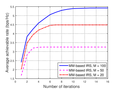
Figure 2: Convergence behaviour of Algorithm 3.

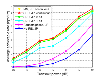
Figure 3: Average achievable rate versus BS transmit power budget.

We first consider a system with only one cell-edge user. We assume that there are two BSs, which are respectively located at $(-300~{}\rm m,0)$ and $(300~{}\rm m,0)$ in the horizontal plane. We assume that the user is located at the middle of a line connecting two BSs, i.e., the user is located at $(0,0)$. Before the performance comparison, we first show the convergence behaviour of Algorithm 3 for the single-user system as shown in Fig. 3. In particular, we show the average achievable rate (average max-min rate for the single-user systems) versus the number of iterations for the different number of IRS reflecting elements, namely $M=20$, $M=50$, and $M=100$, under $N_{t}=2$ and $P_{\rm max}=1~{}\rm W$. It is observed that the average achievable rate obtained by the different number of reflecting elements all increases quickly with the number of iterations. For a large number of reflecting elements, i.e., $M=100$, the proposed algorithm converges within $10$ iterations. Especially, for a small number of reflecting elements, i.e., $M=20$, the proposed algorithm converges in about $4$ iterations as the feasible solution set is smaller. This demonstrates the fast convergence of the proposed Algorithm 3.

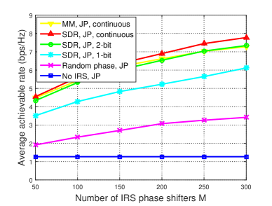
Figure 4: Average achievable rate versus the number of IRS reflecting elements under $N_{t}=2$.

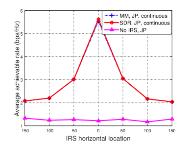
Figure 5: The impact of IRS location on the user’s average achievable rate.

In order to show the performance gain brought by the IRS in the JP-CoMP transmission system, we compare the following schemes: 1) MM, JP, continuous: our proposed Algorithm 3; 2) SDR, JP: this is realized by our proposed scheme, while the difference from scheme 1) lies in the phase shift matrix which is solved based on the SDR technique as discussed in Section IV for the case of multiuser; 3) Random phase, JP: each phase shift at the IRS is random and follows uniform distribution over $\left[{0{\kern 1.0pt}{\kern 1.0pt}{\kern 1.0pt}{\kern 1.0pt}{\kern 1.0pt}2\pi}\right)$ for each channel generation; 4) No IRS, JP: without using the IRS. For scheme “SDR, JP”, we further consider two resolutions of phase shifts, namely $b=1$ and $b=2$. In Fig. 3, we compare the average achievable rate obtained by the above schemes versus the BS transmit power budget under $M=100$ and $N_{t}=2$. It is observed that the average achievable rate obtained by all the schemes increases with the BS transmit power budget. Besides, both the “MM, JP, continuous” and “SDR, JP” schemes outperform the “No IRS, JP” scheme significantly, which demonstrates that the system performance can indeed be improved significantly with the deployment of an IRS. It is also observed that “SDR, JP” with discrete phase shifts suffers from some performance losses compared to the “SDR, JP, continuous” scheme. However, the performance loss can be compensated by adopting a high-resolution phase shifts. Furthermore, the IRS adopting random phase shifts still outperforms the scheme without IRS, as the IRS is able to reflect some of the dissipated signals back to the desired users. Finally, the “MM, JP, continuous” scheme achieves nearly the same performance as the “SDR, JP, continuous” scheme, but with much lower computational complexity as discussed in Section III-C and Section IV-C.

In Fig. 5, the average achievable rate obtained by all the schemes versus the number of IRS reflecting elements is studied. It is observed that the proposed schemes including “SDR, JP” and “MM, JP, continuous” outperform that of both the “Random phase, JP” scheme and the “No IRS, JP” scheme. Especially, for a larger $M$, the system performance gain is more pronounced. For example, when $M=50$, the average rate achieved by the “No IRS” scheme is about 1.29$~{}\rm{bps/Hz}$ and that by “SDR, JP, continuous” scheme is about 4.62$~{}\rm{bps/Hz}$, while when $M=300$, the latter increases up to 7.76$~{}\rm{bps/Hz}$. This is because installing more passive reflecting elements provides more degrees of freedom for resource allocation, which is beneficial for achieving higher beamforming gain, thereby improve the system throughput. More importantly, since the IRS is passive with low power consumption and low cost, it is promising for applying an IRS with hundreds even thousands of reflecting elements.

In Fig. 5, we study the impact of IRS’s location on the user’s average achievable rate under $M=100$ and $N_{t}=2$. We assume that the IRS locates at right above the line connecting two BSs, and the horizontal axis ranges from $\left[{{\rm{-}}150~{}{\rm{m}},150~{}{\rm{m}}}\right]$. It is observed that as the IRS is deployed closer to the user, a higher rate can be achieved due to the smaller reflection path loss. This indicates the potential performance gain brought by the deployment of IRS, especially when IRS is close to the user.

V-B Multiuser System

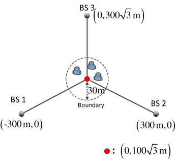
Figure 6: Simulation setup for the multiuser system.

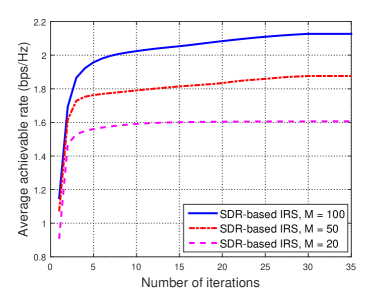
Figure 7: Iteration behaviour of Algorithm 4.

Next, we consider the multiuser system, where there are three BSs and three cell-edge users as shown in Fig. 7. The three BSs are respectively located at $\left({{\rm{-}}300~{}{\rm{m}},0}\right)$, $\left({300~{}{\rm{m}},0}\right)$, and $\left({0,300\sqrt{3}~{}{\rm{m}}}\right)$. Moreover, all the users are uniformly and randomly distributed in a circle centered at $\left({0,100\sqrt{3}~{}{\rm{m}}}\right)$ with a radius $30~{}\rm m$. The IRS is right above the central point $\left({0,100\sqrt{3}~{}{\rm{m}}}\right)$ with altitude $10~{}\rm m$. Unless otherwise stated, we set $N_{t}=6$, $N_{r}=2$, $M=100$ for this scenario.

To show the efficiency of proposed Algorithm 4, its iteration behaviour for the different numbers of the IRS reflecting elements is plotted in Fig. 7. It is observed that the average max-min rate increases quickly with the number of iterations. In particular, for $M=20$, the proposed algorithm terminates in about $5$ iterations, while for $M=100$, only about $25$ iterations are required for reaching the termination.

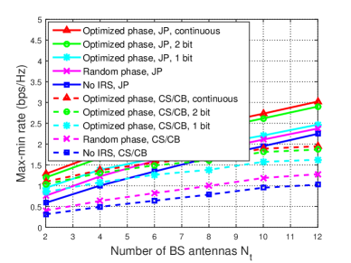
Figure 8: Average max-min rate versus the number of BS antenna $N_{t}$.

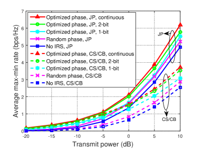
Figure 9: Average max-min rate versus BS transmit power budget.

In order to show the performance gain brought by the IRS-aided JP-CoMP design, the IRS-aided CS/CB-CoMP design proposed in [30] is considered here for comparison. We compare the following schemes for the JP-CoMP systems: 1) Optimized phase, JP: proposed Algorithm 4 in Section IV for the JP-CoMP systems; 2) Random phase, JP: each phase shift at the IRS is randomly chosen from the uniform distribution over $\left[{0{\kern 1.0pt}{\kern 1.0pt}{\kern 1.0pt}{\kern 1.0pt}{\kern 1.0pt}2\pi}\right)$ in each channel generation; 3) No IRS, JP: without adopting the IRS in the JP-CoMP systems. Similarly, we have the same counterpart schemes for the CS/CB-CoMP systems. Also as in Section V-A, we consider both $b=1$ and $b=2$ for the discrete phase shifts at the IRS. In Fig. 9, the average max-min rate obtained by all the schemes versus number of BS antennas is plotted. It is observed that the average max-min rate obtained by all the schemes increases with the number of BS antennas. One can observe that the proposed “Optimized phase, JP, 2-bit” scheme only suffers from a very small performance loss as compared to that the scheme with continuous phase shifts. This shows the great benefits of array gain brought by the multiple number of antennas. In addition, we can also see that our JP schemes outperform their counterpart CS/CB schemes in terms of average max-min rate as the proposed scheme can fully utilize the specific degrees of freedom in the system for resource allocation.

In Fig. 9, we compare the average max-min rate versus the BS transmit power budget. It is firstly observed from Fig. 9 that in terms of the average max-min data rate, the optimized phase schemes for the JP-CoMP design substantially outperform that for the CS/CB-CoMP design, which demonstrates the superiority of the proposed IRS-aided JP-CoMP design. Particularly, when the BS has a larger transmit power budget, the performance gap between two designs becomes more pronounced. This is because inter-user interference can be significantly suppressed by the JP-CoMP technique such that the resource allocation can fully exploit a large transmit power budget at each BS to improve the average max-min rate. For example, when $P_{\rm max}=10~{}{\rm dB}$, the average max-min rate obtained by “Optimized phase, CS/CB, continuous” is $3.7246~{}{\rm bps/Hz}$, and that obtained by “Optimized phase, JP, continuous” is $6.1837~{}{\rm bps/Hz}$, which shows a nearly $40\%$ increase. Besides, one can observe that the average max-min rate of using discrete phase shifts is significantly higher than that without IRS for large transmit power at the BS, which demonstrates the advantage of optimizing phase shifts. We can also see that adopting the IRS with discrete phase shifts suffers some small performance losses compared to the IRS with continuous phase shifts for both designs. This is expected since the multi-path signals cannot be perfectly aligned in phase at receivers in the case with discrete phase shifters, thus resulting in some performance losses. However, with a higher resolution IRS, i.e., $b=2$, the performance loss has been significantly reduced compared to the IRS with continuous phase shifts.

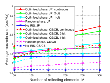
Figure 10: Average max-min rate versus the number of IRS reflecting elements.

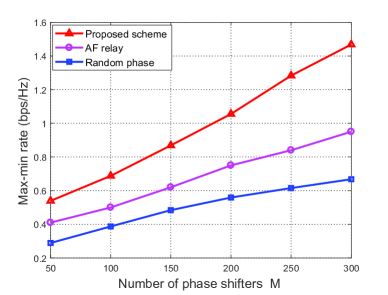
Figure 11: Comparison between the IRS and the AF relay.

In Fig. 11, the average max-min rate versus the number of IRS reflecting elements is studied. It is observed that the performance gain of the IRS-aided JP-CoMP scheme increases as the number of IRS reflecting elements increases, since more reflecting elements help achieve higher passive beamforming gain. In addition, we can observe that the performance gap between “Optimized phase, JP, continuous” and “No IRS, JP” is magnified as $M$ increases. This is because the beam reflected by the IRS towards the desired users becomes more focused and powerful with increasing $M$. This again shows that deploying IRS is a promising solution to address the network capacity bottleneck issue. In addition, we can still observe that the JP-CoMP design outperforms the CS/CB-CoMP design in terms of average max-min rate, especially with large $M$, which further demonstrates the superiority of our proposed JP-CoMP design over the CS/CB-CoMP design. These findings also reinforce also the motivation of our paper, that the combination of JP-CoMP and IRS provides symbiotic benefits to improve the system performance.

Finally, we compare the average max-min rate of the IRS versus the half-duplex amplify-and-forward (AF) relay. To focus on the comparison with large reflecting elements $M$, the direct link from the BS to the user is ignored. Note that [20], [21], [58], and [59] only focus a single-cell system with single-antenna at the receiver, while our work focuses on a more complex multicell multi-antenna multiple user system. For the half duplex AF relaying protocol, the transmission is divided into two equal-sized phases. In the first phase, the data received by the AF relay is

$${{\bf{y}}_{r}}=\sum\limits_{n=1}^{N}{{{\bf{G}}_{n,r}}}{{\bf{x}}_{n}}+{{\bf{n}}_{r}}=\sum\limits_{j=1}^{K}{{{\bf{G}}_{r}}{{\bf{W}}_{j}}}{{\bf{s}}_{j}}+{{\bf{n}}_{r}},$$ (67)

where ${{\bf{G}}_{r}}=\left[{{{\bf{G}}_{1,r}},\ldots,{{\bf{G}}_{N,r}}}\right]$, ${{{\bf{W}}_{j}}}$ is defined in Section II, and ${{\bf{n}}_{r}}\sim{\cal CN}\left({{\bf{0}},{\sigma^{2}}{{\bf{I}}_{{M}}}}\right)$ is the received noise. In the second phase, the relay transmits data to the users, the received signal at user $k$ is given by

$${\bf{y}}_{r}^{{\rm{AF}}} ={{\bf{H}}_{r,k}}{\bf{V}}{{\bf{y}}_{r}}+{{\bf{n}}_{k}}$$

$$={{\bf{H}}_{r,k}}{\bf{V}}\sum\limits_{j=1}^{K}{{{\bf{G}}_{r}}{{\bf{W}}_{j}}}{{\bf{s}}_{j}}+{{\bf{H}}_{r,k}}{\bf{V}}{{\bf{n}}_{r}}+{{\bf{n}}_{k}},$$ (68)

where ${\bf{V}}\in{{\mathbb{C}}^{M\times M}}$ is the relay processing matrix. To compare with the IRS fairly, the analog beamforming matrix is considered, i.e., $\left({i,j}\right)$th element of ${\bf{V}}$ satisfies $\left|{{{\bf{V}}_{i,j}}}\right|=1$.

As a result, the achievable data rate (nat/s/Hz) of user $k$ is given by

$$R_{k}^{{\rm{AF}}}=\frac{1}{2}\ln\left|{{{\bf{I}}_{{N_{r}}}}+{{\bf{H}}_{r,k}}{\bf{V}}{{\bf{G}}_{r}}{{\bf{W}}_{k}}{\bf{W}}_{k}^{H}{\bf{G}}_{r}^{H}{{\bf{V}}^{H}}{\bf{H}}_{r,k}^{H}{\bf{F}}_{2,k}^{-1}}\right|,$$ (69)

where ${{\bf{F}}_{2,k}}={{\bf{H}}_{r,k}}{\bf{V}}\left({{{\bf{G}}_{r}}\sum\limits_{j\neq k}^{K}{{{\bf{W}}_{j}}{\bf{W}}_{j}^{H}}{\bf{G}}_{r}^{H}+{\sigma^{2}}{{\bf{I}}_{M}}}\right){{\bf{V}}^{H}}{\bf{H}}_{r,k}^{H}+{\sigma^{2}}{{\bf{I}}_{M}}$, the factor $\frac{1}{2}$ denotes the half-duplex protocol adopted at the relay. As such, we have the following problem for the half-duplex AF relaying systems:

$$\left({\rm{P}3}\right): \mathop{\rm maximize}\limits_{{{\bf{W}}_{n,k}},{\bf V},R}{\kern 1.0pt}{\kern 1.0pt}{\kern 1.0pt}{\kern 1.0pt}R$$

$${\rm s.t.}~{}\frac{1}{2}\ln\left|{{{\bf{I}}_{{N_{r}}}}+{{\bf{H}}_{r,k}}{\bf{V}}{{\bf{G}}_{r}}{{\bf{W}}_{k}}{\bf{W}}_{k}^{H}{\bf{G}}_{r}^{H}{{\bf{V}}^{H}}{\bf{H}}_{r,k}^{H}{\bf{F}}_{2,k}^{-1}}\right|$$

$$\qquad\qquad\qquad\qquad\qquad\qquad\qquad\geq R,k\in\cal{\cal K},$$ (70)

$$\qquad\sum\limits_{k=1}^{K}{\left\|{{{\bf{W}}_{n,k}}}\right\|_{F}^{2}}\leq{P_{\max}},{\kern 1.0pt}{\kern 1.0pt}n\in\cal N,$$ (71)

$$\qquad\left|{{{\bf{V}}_{i,j}}}\right|=1,i\in{\cal M},j\in{\cal M}.$$ (72)

Problem $({\rm P}3)$ is different from $({\rm P}3)$, where the non-diagonal element of ${\bf{V}}$ is constrained to modulus $1$. To solve Problem $({\rm P}3)$, MSE and alternating optimization method are still applied. Specifically, for the given analog beamforming ${\bf{V}}$, the BS beamforming ${{{\bf{W}}_{n,k}}}$ can be solved similar to Section IV-A. As for the given BS beamforming ${{{\bf{W}}_{n,k}}}$, analog beamforming ${\bf{V}}$ can be solved by updating each phase shift sequentially according to [29]. In Fig. 11, we plot the average max-min rate versus the number of IRS reflecting elements for the IRS and the AF relay. It is observed that proposed scheme (i.e., optimize IRS phase shift) outperforms that of AF relaying. Specifically, when the number of reflecting elements $M$ is small, the performance gap between proposed scheme and AF relaying is small. However, when $M$ is large, the performance gap becomes significant. Since the IRS is passive, the signal impinging on IRS is directly reflected with no time delay due to its passive property, while the signal impinges on relay, a time slot delay is induced due to the active components applied at relay.

VI Conclusion

In this paper, we studied the IRS-aided JP-CoMP downlink transmission in multi-cell systems. To guarantee the user fairness, a max-min rate problem was formulated by jointly optimizing the IRS phase shift matrix and the BS transmit beamforming matrix. We considered both the single cell-edge user system and multi-user system. For the single-user system, the transmit beamforming matrix was optimally obtained based on the subgradient method for the fixed IRS phase shift matrix, and the IRS phase shift matrix was obtained based on the MM method for the fixed transmit beamforming matrix. Exploiting these two solutions, an efficient iterative resource allocation algorithm was proposed. For the multi-user system, with the given phase shift matrix, the transmit beamforming optimization problem was transformed into an SOCP, which was efficiently solved by the interior point method. For the given transmit beamforming matrix, the IRS phase shift matrix was optimized by leveraging the SDR technique. Then, an efficient iterative algorithm was also proposed. Simulation results demonstrated that with the deployment of IRS, significant throughput can be achieved over the case without IRS. Furthermore, the proposed JP-CoMP design significantly outperforms the CS/CB-CoMP design in terms of max-min rate. The results in this paper can be further extended by considering multiple IRSs, frequency-selective channel model, imperfect CSI, etc., which will be left as future work.

APPENDIX A

We prove the theorem by examing the Karush-Kuhn-Tucker (KKT) conditions of both $(\rm P)$ and $(\rm P1)$. We first show that the KKT conditions of problem $\left({\rm{P}}\right)$ is the same as that of $\left({\rm{P1}}\right)$. To start with, the Lagrangian function associated with constraint (10) of $\left({\rm{P1}}\right)$ is given by

$${\cal L}\left({{{\bf{W}}_{n,k}},{\theta_{m}},R,{{\bf{U}}_{k}},{{\bf{Q}}_{k}},{\lambda_{k}}}\right)=R$$

$$+\sum\limits_{k=1}^{K}{{\lambda_{k}}}\left({\ln\left|{{{\bf{Q}}_{k}}}\right|-{\rm{Tr}}\left({{{\bf{Q}}_{k}}{{\bf{E}}_{k}}}\right)+d-R}\right),$$ (73)

where $\lambda_{k}\geq 0$, $\forall k$, is the dual variable corresponding to constraint (10). According to [49], all the locally optimal solutions (including the globally optimal solutions) must satisfy the KKT conditions. Specifically, by setting the first-order derivative of $\cal L$ with respect to variables ${{{\bf{Q}}_{k}}}$ and ${{\bf U}_{k}}$ to zero, we have

$${\nabla_{{{\bf{Q}}_{k}}}}{\cal L}\left({{{\bf{W}}_{n,k}},{\theta_{m}},R,{{\bf{U}}_{k}},{{\bf{Q}}_{k}},{\lambda_{k}}}\right)={\bf 0},$$ (74)

$${\nabla_{{{\bf{U}}_{k}}}}{\cal L}\left({{{\bf{W}}_{n,k}},{\theta_{m}},R,{{\bf{U}}_{k}},{{\bf{Q}}_{k}},{\lambda_{k}}}\right)={\bf 0},$$ (75)

respectively. Based on (74) and (75), the optimal solutions ${{{\bf{Q}}_{k}^{\rm opt}}}$ and ${{{\bf{U}}_{k}^{\rm opt}}}$ can be derived as

$${\bf{Q}}_{k}^{\rm opt}={\bf{E}}_{k}^{-1},$$ (76)

$${\bf{U}}_{k}^{\rm opt}={\left({{{{\bf{\bar{H}}}}_{k}}\left({\sum\limits_{j=1}^{K}{{{\bf{W}}_{j}}{\bf{W}}_{j}^{H}}}\right){\bf{\bar{H}}}_{k}^{H}+{\sigma^{2}}{\bf{I}}_{N_{r}}}\right)^{-1}}{{{\bf{\bar{H}}}}_{k}}{{\bf{W}}_{k}}.$$ (77)

Substituting (77) into (9), the minimum MSE (MMSE) matrix is given by

$${\bf{E}}_{k}^{\rm mmse}={\bf{I}}_{d}-{\bf{W}}_{k}^{H}{\bf{\bar{H}}}_{k}^{H}{\bf{J}}_{k}^{-1}{{{\bf{\bar{H}}}}_{k}}{{\bf{W}}_{k}},$$ (78)

where ${{\bf{J}}_{k}}=\left({{{{\bf{\bar{H}}}}_{k}}\left({\sum\limits_{j=1}^{K}{{{\bf{W}}_{j}}{\bf{W}}_{j}^{H}}}\right){\bf{\bar{H}}}_{k}^{H}+{\sigma^{2}}{\bf{I}}_{N_{r}}}\right)$. Then, substituting (76) and (77) into (73), we arrive at

$${\cal L}\left({{{\bf{W}}_{n,k}},{\theta_{m}},R,{\lambda_{k}}}\right)=R+\sum\limits_{k=1}^{K}{{\lambda_{k}}}\left({\ln\left|{{{\left({{\bf{E}}_{k}^{\rm mmse}}\right)}^{-1}}}\right|}-R\right).$$ (79)

Using the Duncan-Guttman formula ${\left({{\bf{A}}-{\bf{UD^{-1}V}}}\right)^{-1}}={{\bf{A}}^{-1}}+{{\bf{A}}^{-1}}{\bf{U}}{\left({{\bf{D}}-{\bf{V}}{{\bf{A}}^{-1}}{\bf{U}}}\right)^{-1}}{\bf{V}}{{\bf{A}}^{-1}}$ [50], we can rewrite (79) as

$${\cal L}\left({{{\bf{W}}_{n,k}},{\theta_{m}},R,{\lambda_{k}}}\right)=R$$

$$+\sum\limits_{k=1}^{K}{{\lambda_{k}}}\left({\ln\left|{{\bf{I}}_{N_{r}}+{{{\bf{\bar{H}}}}_{k}}{{\bf{W}}_{k}}{\bf{W}}_{k}^{H}{\bf{\bar{H}}}_{k}^{H}{\bf{F}}_{k}^{-1}}\right|}-R\right).$$ (80)

It can be seen that (80) is also a Lagrangian function of $\left({\rm{P}}\right)$ provided that $\lambda_{k}$ is the Lagrangian multipliers for constraint (5). This indicates that problems $\left({\rm{P}}\right)$ and $\left({\rm{P1}}\right)$ have the same optimal primal solution, which thus completes the proof of Theorem 1.

APPENDIX B

With the identity ${\rm{Tr}}\left({{\bf{AB}}}\right)={\left({{\rm{vec}}\left({\bf{A}}\right)}\right)^{H}}{\rm{vec}}\left({\bf{B}}\right)$ [50], we have $\left\|{{{\bf{W}}_{n,k}}}\right\|_{F}^{2}{\rm{=Tr}}\left({{\bf{W}}_{n,k}^{H}{{\bf{W}}_{n,k}}}\right)={\left({{\rm{vec}}\left({{{\bf{W}}_{n,k}}}\right)}\right)^{H}}{\rm{vec}}\left({{{\bf{W}}_{n,k}}}\right)$. Therefore, we can rewrite (6) as

$${\left\|{{{\bm{\eta}}_{n}}}\right\|_{2}}\leq\sqrt{{P_{\max}}},\forall n,$$ (81)

where ${{{\bm{\eta}}_{n}}}$ is given by

$${{\bm{\eta}}_{n}}={\left[{{{\left({{\rm{vec}}\left({{{\bf{W}}_{n,1}}}\right)}\right)}^{H}},\cdots,{{\left({{\rm{vec}}\left({{{\bf{W}}_{n,K}}}\right)}\right)}^{H}}}\right]^{H}}.$$ (82)

For constraint (10), we first rewrite ${{\bf{E}}_{k}}$ in (9) as

$${{\bf{E}}_{k}}=\left({{\bf{U}}_{k}^{H}{{{\bf{\bar{H}}}}_{k}}{{\bf{W}}_{k}}-{\bf{I}}}\right){\left({{\bf{U}}_{k}^{H}{{{\bf{\bar{H}}}}_{k}}{{\bf{W}}_{k}}-{\bf{I}}}\right)^{H}}$$

$$+{\bf{U}}_{k}^{H}{{{\bf{\bar{H}}}}_{k}}\left({\sum\limits_{j\neq k}^{K}{{{\bf{W}}_{j}}{\bf{W}}_{j}^{H}}}\right){\bf{\bar{H}}}_{k}^{H}{{\bf{U}}_{k}}+{\sigma^{2}}{\bf{U}}_{k}^{H}{{\bf{U}}_{k}}.$$ (83)

Substituting (83) into (10), we have

$${\left\|{{{\bm{\omega}}_{k}}}\right\|_{2}}\leq\sqrt{\ln\left|{{{\bf{Q}}_{k}}}\right|+d-R-{\sigma^{2}}{\rm{Tr}}\left({{{\bf{Q}}_{k}}{\bf{U}}_{k}^{H}{{\bf{U}}_{k}}}\right)},\forall k,$$ (84)

where ${{\bm{\omega}}_{k}}$ is given by

$${{\bm{\omega}}_{k}} =\left[{{{\left({{\rm{vec}}\left({{\bf{W}}_{1}^{H}{\bf{\bar{H}}}_{k}^{H}{{\bf{U}}_{k}}{\bf{Q}}_{k}^{1/2}}\right)}\right)}^{H}}}\right.$$

$$,\cdots,{\left({{\rm{vec}}\left({{\bf{W}}_{k}^{H}{\bf{\bar{H}}}_{k}^{H}{{\bf{U}}_{k}}{\bf{Q}}_{k}^{1/2}-{\bf{Q}}_{k}^{1/2}}\right)}\right)^{H}}$$

$$,\cdots,{\left.{{{\left({{\rm{vec}}\left({{\bf{W}}_{K}^{H}{\bf{\bar{H}}}_{k}^{H}{{\bf{U}}_{k}}{\bf{Q}}_{k}^{1/2}}\right)}\right)}^{H}}}\right]^{H}}.$$ (85)

This completes the proof of Theorem 2.

Meng Hua received the M.S. degree in electrical and information engineering from Nanjing University of Science and Technology, Nanjing, China, in 2016. Since September 2016, he is currently working towards the Ph.D. degree in School of Information Science and Engineering, Southeast University, Nanjing, China. His current research interests include UAV assisted communication, intelligent reflecting surface (IRS), backscatter communication, energy-efficient wireless communication, X-connectivity, cognitive radio network, secure transmission, and optimization theory.

Qingqing Wu (S’13-M’16) received the B.Eng. and the Ph.D. degrees in Electronic Engineering from South China University of Technology and Shanghai Jiao Tong University (SJTU) in 2012 and 2016, respectively. He is currently an Assistant Professor in the Department of Electrical and Computer Engineering at the University of Macau, China, and also with the State key laboratory of Internet of Things for Smart City. He was a Research Fellow in the Department of Electrical and Computer Engineering at National University of Singapore. His current research interest includes intelligent reflecting surface (IRS), unmanned aerial vehicle (UAV) communications, and MIMO transceiver design. He has published over 80 IEEE journal and conference papers. He was the recipient of the IEEE WCSP Best Paper Award in 2015, the Outstanding Ph.D. Thesis Funding in SJTU in 2016, the Outstanding Ph.D. Thesis Award of China Institute of Communications in 2017. He was the Exemplary Editor of IEEE Communications Letters in 2019 and the Exemplary Reviewer of several IEEE journals. He serves as an Associate Editor for IEEE Communications Letters and IEEE Open Journal of Communications Society. He is the Lead Guest Editor for IEEE Journal on Selected Areas in Communications on “UAV Communications in 5G and Beyond Networks”, and the Guest Editor for IEEE Open Journal on Vehicular Technology on “6G Intelligent Communications” and IEEE Open Journal of Communications Society on “Reconfigurable Intelligent Surface-Based Communications for 6G Wireless Networks”. He is the workshop co-chair for ICC 2019 and ICC 2020 workshop on “Integrating UAVs into 5G and Beyond”, and the workshop co-chair for GLOBECOM 2020 workshop on “Reconfigurable Intelligent Surfaces for Wireless Communication for Beyond 5G”.

Derrick Wing Kwan Ng (S’06-M’12-SM’17-F’21) received the bachelor degree with first-class honors and the Master of Philosophy (M.Phil.) degree in electronic engineering from the Hong Kong University of Science and Technology (HKUST) in 2006 and 2008, respectively. He received his Ph.D. degree from the University of British Columbia (UBC) in 2012. He was a senior postdoctoral fellow at the Institute for Digital Communications, Friedrich-Alexander-University Erlangen-Nürnberg (FAU), Germany. He is now working as a Senior Lecturer and a Scientia Fellow at the University of New South Wales, Sydney, Australia. His research interests include convex and non-convex optimization, physical layer security, IRS-assisted communication, UAV-assisted communication, wireless information and power transfer, and green (energy-efficient) wireless communications. Dr. Ng received the Australian Research Council (ARC) Discovery Early Career Researcher Award 2017, the Best Paper Awards at the IEEE TCGCC Best Journal Paper Award 2018, INISCOM 2018, IEEE International Conference on Communications (ICC) 2018, IEEE International Conference on Computing, Networking and Communications (ICNC) 2016, IEEE Wireless Communications and Networking Conference (WCNC) 2012, the IEEE Global Telecommunication Conference (Globecom) 2011, and the IEEE Third International Conference on Communications and Networking in China 2008. He has been serving as an editorial assistant to the Editor-in-Chief of the IEEE Transactions on Communications from Jan. 2012 to Dec. 2019. He is now serving as an editor for the IEEE Transactions on Communications, the IEEE Transactions on Wireless Communications, and an area editor for the IEEE Open Journal of the Communications Society. Also, he has been listed as a Highly Cited Researcher by Clarivate Analytics since 2018. He is an IEEE Fellow.

Jun Zhao (S’10-M’15) is currently an Assistant Professor in the School of Computer Science and Engineering at Nanyang Technological University (NTU) in Singapore. He received a PhD degree in May 2015 in Electrical and Computer Engineering from Carnegie Mellon University (CMU) in the USA (advisors: Virgil Gligor, Osman Yagan; collaborator: Adrian Perrig), affiliating with CMU’s renowned CyLab Security & Privacy Institute, and a bachelor’s degree in July 2010 from Shanghai Jiao Tong University in China. Before joining NTU first as a postdoc with Xiaokui Xiao and then as a faculty member, he was a postdoc at Arizona State University as an Arizona Computing PostDoc Best Practices Fellow (advisors: Junshan Zhang, Vincent Poor). His research interests include communication networks, security/privacy, and AI. His co-authored papers received Best Paper Award (IEEE Transaction Paper) by IEEE Vehicular Society (VTS) Singapore Chapter in 2019, and Best Paper Award in EAI International Conference on 6G for Future Wireless Networks (EAI 6GN) 2020.

Luxi Yang (M’96-SM’17) received the M.S. and Ph.D. degrees in electrical engineering from Southeast University, Nanjing, China, in 1990 and 1993, respectively. Since 1993, he has been with the Department of Radio Engineering, Southeast University, where he is currently a Full Professor of information systems and communications, and the Director of the Digital Signal Processing Division. He has authored or co-authored of two published books and more than 200 journal papers, and holds 50 patents. His current research interests include signal processing for wireless communications, MIMO communications, intelligent wireless communications, and statistical signal processing. He received the first and second class prizes of science and technology progress awards of the State Education Ministry of China in 1998, 2002, and 2014. He is currently a member of Signal Processing Committee of the Chinese Institute of Electronics.

References

- [1] L. Lu, G. Y. Li, A. L. Swindlehurst, A. Ashikhmin, and R. Zhang, “An overview of massive MIMO: Benefits and challenges,” IEEE J. Sel. Top. Sign. Proces., vol. 8, no. 5, pp. 742–758, Oct. 2014.
- [2] E. G. Larsson, O. Edfors, F. Tufvesson, and T. L. Marzetta, “Massive MIMO for next generation wireless systems,” IEEE Commun. Mag., vol. 52, no. 2, pp. 186–195, Feb. 2014.
- [3] A. L. Swindlehurst, E. Ayanoglu, P. Heydari, and F. Capolino, “Millimeter-wave massive MIMO: The next wireless revolution?” IEEE Commun. Mag., vol. 52, no. 9, pp. 56–62, Sep. 2014.
- [4] M. Kamel, W. Hamouda, and A. Youssef, “Ultra-dense networks: A survey,” IEEE Commun. Surveys Tuts., vol. 18, no. 4, pp. 2522–2545, 4th Quat. 2016.
- [5] V. W. Wong, D. W. K. Ng, R. Schober, and L.-C. Wang, Key technologies for 5G wireless systems. Cambridge university press, 2017.
- [6] X. Chen, D. W. K. Ng, W. Yu, E. G. Larsson, N. Al-Dhahir, and R. Schober, “Massive access for 5G and beyond,” 2020. [Online]. Available: https://arxiv.org/abs/2002.03491.
- [7] S. Zhang, Q. Wu, S. Xu, and G. Y. Li, “Fundamental green tradeoffs: Progresses, challenges, and impacts on 5G networks,” IEEE Commun. Surveys Tuts., vol. 19, no. 1, pp. 33–56, 1st Quat. 2017.
- [8] Q. Wu, G. Y. Li, W. Chen, D. W. K. Ng, and R. Schober, “An overview of sustainable green 5G networks,” IEEE Wireless Commun., vol. 24, no. 4, pp. 72–80, Aug. 2017.
- [9] Q. Wu and R. Zhang, “Towards smart and reconfigurable environment: Intelligent reflecting surface aided wireless network,” IEEE Commun. Mag., vol. 58, no. 1, pp. 106–112, Jan. 2020.
- [10] E. Basar, M. Di Renzo, J. De Rosny, M. Debbah, M.-S. Alouini, and R. Zhang, “Wireless communications through reconfigurable intelligent surfaces,” IEEE Access, vol. 7, pp. 116 753–116 773, 2019.
- [11] J. Zhao, “A survey of intelligent reflecting surfaces (IRSs): Towards 6G wireless communication networks with massive MIMO 2.0.” [Online]. Available: https://arxiv.org/abs/1907.04789.
- [12] J. Zhang, E. Björnson, M. Matthaiou, D. W. K. Ng, H. Yang, and D. J. Love, “Prospective multiple antenna technologies for beyond 5G,” IEEE J. Sel. Areas Commun., vol. 38, no. 8, pp. 1637–1660, Aug. 2020.
- [13] T. J. Cui, S. Liu, and L. Zhang, “Information metamaterials and metasurfaces,” J. Phys. Chem. C, vol. 5, no. 15, pp. 3644–3668, 2017.
- [14] T. J. Cui, M. Q. Qi, X. Wan, J. Zhao, and Q. Cheng, “Coding metamaterials, digital metamaterials and programmable metamaterials,” Light Sci. Appl., vol. 3, no. 10, p. e218, Oct. 2014.
- [15] P. Nayeri, F. Yang, and A. Z. Elsherbeni, Reflectarray Antennas: Theory, Designs, and Applications. John Wiley & Sons, 2018.
- [16] C. Liaskos, S. Nie, A. Tsioliaridou, A. Pitsillides, S. Ioannidis, and I. Akyildiz, “Realizing wireless communication through software-defined hypersurface environments,” in 2018 IEEE 19th International Symposium on ”A World of Wireless, Mobile and Multimedia Networks” (WoWMoM), 2018, pp. 14–15.
- [17] Q. Ma, G. D. Bai, H. B. Jing, C. Yang, L. Li, and T. J. Cui, “Smart metasurface with self-adaptively reprogrammable functions,” Light-Science & Applications, vol. 8, no. 1, pp. 1–12, 2019.
- [18] C. Liaskos, S. Nie, A. Tsioliaridou, A. Pitsillides, S. Ioannidis, and I. Akyildiz, “A new wireless communication paradigm through software-controlled metasurfaces,” IEEE Commun. Mag., vol. 56, no. 9, pp. 162–169, 2018.
- [19] C. Huang, S. Hu, G. C. Alexandropoulos, A. Zappone, C. Yuen, R. Zhang, M. Di Renzo, and M. Debbah, “Holographic mimo surfaces for 6G wireless networks: Opportunities, challenges, and trends,” IEEE Wireless Commun., 2020, early access, doi: 10.1109/MWC.001.1900534.
- [20] C. Huang, A. Zappone, G. C. Alexandropoulos, M. Debbah, and C. Yuen, “Reconfigurable intelligent surfaces for energy efficiency in wireless communication,” IEEE Trans. Wireless Commun., vol. 18, no. 8, pp. 4157–4170, 2019.
- [21] Q. Wu and R. Zhang, “Intelligent reflecting surface enhanced wireless network via joint active and passive beamforming,” IEEE Trans. Wireless Commun., vol. 18, no. 11, pp. 5394–5409, Nov. 2019.
- [22] B. O. Zhu, J. Zhao, and Y. Feng, “Active impedance metasurface with full 360 reflection phase tuning,” Scientific Reports, vol. 3, 2013.
- [23] T.-J. Cui, S. Liu, and L.-L. Li, “Information entropy of coding metasurface,” Light Science & Applications, vol. 5, no. 11, p. e16172, 2016.
- [24] S. Abeywickrama, R. Zhang, Q. Wu, and C. Yuen, “Intelligent reflecting surface: Practical phase shift model and beamforming optimization,” IEEE Trans. Commun., vol. 68, no. 9, pp. 5849–5863, Sept. 2020.
- [25] W. Tang, M. Z. Chen, X. Chen, J. Y. Dai, Y. Han, M. Di Renzo, Y. Zeng, S. Jin, Q. Cheng, and T. J. Cui, “Wireless communications with reconfigurable intelligent surface: Path loss modeling and experimental measurement,” IEEE Trans. Wireless Commun., 2020, doi: 10.1109/TWC.2020.3024887.
- [26] C. You, B. Zheng, and R. Zhang, “Intelligent reflecting surface with discrete phase shifts: Channel estimation and passive beamforming,” in IEEE International Conference on Communications (ICC), 2020, pp. 1–6.
- [27] J. Mirza and B. Ali, “Channel estimation method and phase shift design for reconfigurable intelligent surface assisted MIMO networks.” [Online]. Available: https://arxiv.org/abs/1912.10671.
- [28] J. Chen, Y.-C. Liang, H. V. Cheng, and W. Yu, “Channel estimation for reconfigurable intelligent surface aided multi-user MIMO systems.” [Online]. Available: https://arxiv.org/abs/1912.03619.
- [29] Q. Wu and R. Zhang, “Beamforming optimization for wireless network aided by intelligent reflecting surface with discrete phase shifts,” IEEE Trans. Commun., vol. 68, no. 3, pp. 1838–1851, Mar. 2020.
- [30] C. Pan, H. Ren, K. Wang, W. Xu, M. Elkashlan, A. Nallanathan, and L. Hanzo, “Multicell MIMO communications relying on intelligent reflecting surface,” IEEE Trans. Wireless Commun., vol. 19, no. 8, pp. 5218–5233, 2020.
- [31] C. Pan, H. Ren, K. Wang, M. Elkashlan, A. Nallanathan, J. Wang, and L. Hanzo, “Intelligent reflecting surface enhanced MIMO broadcasting for simultaneous wireless information and power transfer,” IEEE J. Sel. Areas Commun., vol. 38, no. 8, pp. 1719–1734, Aug. 2020.
- [32] R. Liu, M. Li, Q. Liu, and A. L. Swindlehurst, “Joint symbol-level precoding and reflecting designs for RIS-enhanced MU-MISO systems.” [Online]. Available: https://arxiv.org/abs/1912.11767.
- [33] C. Huang, G. C. Alexandropoulos, A. Zappone, M. Debbah, and C. Yuen, “Energy efficient multi-user MISO communication using low resolution large intelligent surfaces,” in 2018 IEEE Globecom Workshops (GC Wkshps), 2018, pp. 1–6.
- [34] Q. Wu and R. Zhang, “Weighted sum power maximization for intelligent reflecting surface aided SWIPT,” IEEE Wireless Commun. Lett., vol. 9, no. 5, pp. 586–590, May 2020.
- [35] ——, “Joint active and passive beamforming optimization for intelligent reflecting surface assisted SWIPT under QoS constraints,” IEEE J. Sel. Areas Commun., vol. 38, no. 8, pp. 1735–1748, Aug. 2020.
- [36] X. Guan, Q. Wu, and R. Zhang, “Intelligent reflecting surface assisted secrecy communication: Is artificial noise helpful or not?” IEEE Wireless Commun. Lett., Jan. 2020, DOI: 10.1109/LWC.2020.2969629.
- [37] C. Huang, R. Mo, and C. Yuen, “Reconfigurable intelligent surface assisted multiuser MISO systems exploiting deep reinforcement learning,” IEEE J. Sel. Areas Commun., 2020, early access, doi: 10.1109/JSAC.2020.3000835.
- [38] R. Irmer, H. Droste, P. Marsch, M. Grieger, G. Fettweis, S. Brueck, H.-P. Mayer, L. Thiele, and V. Jungnickel, “Coordinated multipoint: Concepts, performance, and field trial results,” IEEE Commun. Mag., vol. 49, no. 2, pp. 102–111, Feb. 2011.
- [39] 3GPP TR 36.814, “Further advancements for E-UTRA physical layer aspects,” Release 9, v. 9.0.0, Mar, 2010.
- [40] H. Q. Ngo, A. Ashikhmin, H. Yang, E. G. Larsson, and T. L. Marzetta, “Cell-free massive MIMO versus small cells,” IEEE Trans. Wireless Commun., vol. 16, no. 3, pp. 1834–1850, Mar. 2017.
- [41] E. Nayebi, A. Ashikhmin, T. L. Marzetta, H. Yang, and B. D. Rao, “Precoding and power optimization in cell-free massive MIMO systems,” IEEE Trans. Wireless Commun., vol. 16, no. 7, pp. 4445–4459, Jul. 2017.
- [42] G. Nigam, P. Minero, and M. Haenggi, “Coordinated multipoint joint transmission in heterogeneous networks,” IEEE Trans. Commun., vol. 62, no. 11, pp. 4134–4146, Nov. 2014.
- [43] J. Tang, A. Shojaeifard, D. K. So, K.-K. Wong, and N. Zhao, “Energy efficiency optimization for CoMP-SWIPT heterogeneous networks,” IEEE Trans. Commun., vol. 66, no. 12, pp. 6368–6383, Dec. 2018.
- [44] Q. Wu, S. Zhang, B. Zheng, C. You, and R. Zhang, “Intelligent reflecting surface aided wireless communications: A tutorial,” 2020. [Online]. Available: https://arxiv.org/abs/2007.02759v1
- [45] J. Kang, O. Simeone, J. Kang, and S. S. Shitz, “Joint signal and channel state information compression for the backhaul of uplink network MIMO systems,” IEEE Trans. Wireless Commun., vol. 13, no. 3, pp. 1555–1567, 2014.
- [46] H. Masoumi and M. J. Emadi, “Performance analysis of cell-free massive mimo system with limited fronthaul capacity and hardware impairments,” IEEE Trans. Wireless Commun., vol. 19, no. 2, pp. 1038–1053, 2020.
- [47] Q. Shi, M. Razaviyayn, Z.-Q. Luo, and C. He, “An iteratively weighted MMSE approach to distributed sum-utility maximization for a MIMO interfering broadcast channel,” IEEE Trans. Signal Process., vol. 59, no. 9, pp. 4331–4340, Sep. 2011.
- [48] M. Grant and S. Boyd, “CVX: Matlab software for disciplined convex programming, version 2.1,” http://cvxr.com/cvx, Mar. 2014.
- [49] S. Boyd and L. Vandenberghe, Convex optimization. Cambridge university press, 2004.
- [50] X.-D. Zhang, Matrix analysis and applications. Cambridge University Press, 2017.
- [51] Y. Sun, P. Babu, and D. P. Palomar, “Majorization-minimization algorithms in signal processing, communications, and machine learning,” IEEE Trans. Signal Process., vol. 65, no. 3, pp. 794–816, Feb. 2016.
- [52] J. Song, P. Babu, and D. P. Palomar, “Sequence design to minimize the weighted integrated and peak sidelobe levels,” IEEE Trans. Signal Process., vol. 64, no. 8, pp. 2051–2064, Apr. 2016.
- [53] M. Hua, Y. Wang, M. Lin, C. Li, Y. Huang, and L. Yang, “Joint CoMP transmission for UAV-aided cognitive satellite terrestrial networks,” IEEE Access, vol. 7, pp. 14 959–14 968, 2019.
- [54] Y. Wang, C. Li, Y. Huang, D. Wang, T. Ban, and L. Yang, “Energy-efficient optimization for downlink massive MIMO FDD systems with transmit-side channel correlation,” IEEE Trans. Veh. Technol., vol. 65, no. 9, pp. 7228–7243, Sep. 2015.
- [55] M. S. Lobo, L. Vandenberghe, S. Boyd, and H. Lebret, “Applications of second-order cone programming,” Linear algebra and its applications, vol. 284, no. 1-3, pp. 193–228, Nov. 1998.
- [56] N. D. Sidiropoulos, T. N. Davidson, and Z.-Q. Luo, “Transmit beamforming for physical-layer multicasting,” IEEE Trans. Signal Process., vol. 54, no. 6, pp. 2239–2251, Jun. 2006.
- [57] C. Pan, H. Zhu, N. J. Gomes, and J. Wang, “Joint precoding and RRH selection for user-centric green MIMO C-RAN,” IEEE Trans. Wireless Commun., vol. 16, no. 5, pp. 2891–2906, May 2017.
- [58] E. Björnson, Ö. Özdogan, and E. G. Larsson, “Intelligent reflecting surface versus decode-and-forward: How large surfaces are needed to beat relaying?” IEEE Wireless Commun. Lett., vol. 9, no. 2, pp. 244–248, 2020.
- [59] M. Di Renzo, K. Ntontin, J. Song, F. H. Danufane, X. Qian, F. Lazarakis, J. De Rosny, D. Phan-Huy, O. Simeone, R. Zhang, M. Debbah, G. Lerosey, M. Fink, S. Tretyakov, and S. Shamai, “Reconfigurable intelligent surfaces vs. relaying: Differences, similarities, and performance comparison,” IEEE Open Journal of the Communications Society, vol. 1, pp. 798–807, 2020.