Autonomous Cave Surveying with an Aerial Robot

Abstract

This paper presents a method for cave surveying in total darkness using an autonomous aerial vehicle equipped with a depth camera for mapping, downward-facing camera for state estimation, and forward and downward lights. Traditional methods of cave surveying are labor-intensive and dangerous due to the risk of hypothermia when collecting data over extended periods of time in cold and damp environments, the risk of injury when operating in darkness in rocky or muddy environments, and the potential structural instability of the subterranean environment. Although these dangers can be mitigated by deploying robots to map dangerous passages and voids, real-time feedback is often needed to operate robots safely and efficiently. Few state-of-the-art, high-resolution perceptual modeling techniques attempt to reduce their high bandwidth requirements to work well with low bandwidth communication channels. To bridge this gap in the state of the art, this work compactly represents sensor observations as Gaussian mixture models and maintains a local occupancy grid map for a motion planner that greedily maximizes an information-theoretic objective function. The approach accommodates both limited field of view depth cameras and larger field of view LiDAR sensors and is extensively evaluated in long duration simulations on an embedded PC. An aerial system is leveraged to demonstrate the repeatability of the approach in a flight arena as well as the effects of communication dropouts. Finally, the system is deployed in Laurel Caverns, a commercially owned and operated cave in southwestern Pennsylvania, USA, and a wild cave in West Virginia, USA. Videos of the simulation and hardware results are available at https://youtu.be/iwi3p7IENjE and https://youtu.be/H8MdtJ5VhyU.

I Introduction

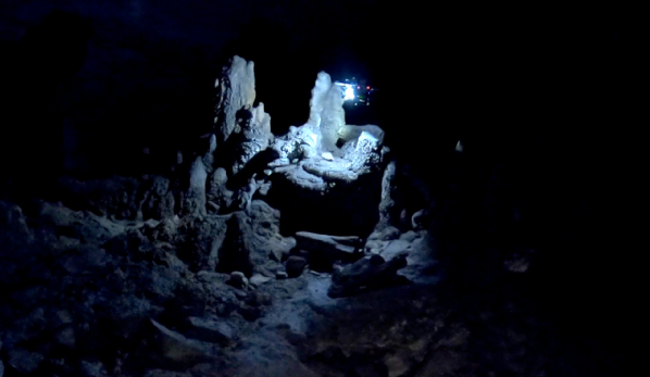
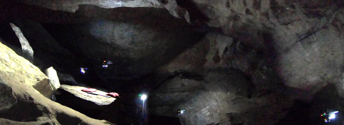
The process of cave surveying, which consists of marking stations and measuring the distances between them, has changed relatively little since the 19th century [1, p. 1532]. While Gunn [1] predicts that advancements in technology may fundamentally change this method in the 21st century, the substantial advancements in sensing, 3D reconstruction, and autonomy made within the last decade have not propagated to cave surveying. This paper addresses this gap in the state of the art through the development and testing of an autonomous aerial system that explores and maps caves (see Fig. 1).

(a)

(b)

(c)

(d)

Figure 1: Data and imagery excerpted from an exploration trial in a cave in West Virginia. LABEL:sub@sfig:robot_mapping An autonomous aerial system explores and maps a formation. LABEL:sub@sfig:rapps_color_camera A color image taken by the aerial system during exploration (the formation shown in LABEL:sub@sfig:robot_mapping can be seen on the left-hand side of LABEL:sub@sfig:rapps_color_camera). A depth image taken at the same time is shown in LABEL:sub@sfig:rapps_depth_camera and the resampled GMM map built during flight from the depth image is shown in LABEL:sub@sfig:rapps_resampled_gmm. The video of the exploration trial corresponding to these images may be found at https://youtu.be/H8MdtJ5VhyU

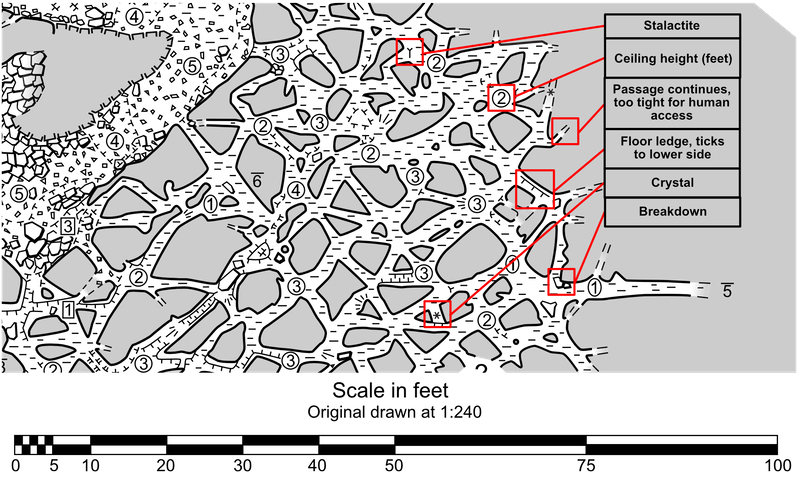
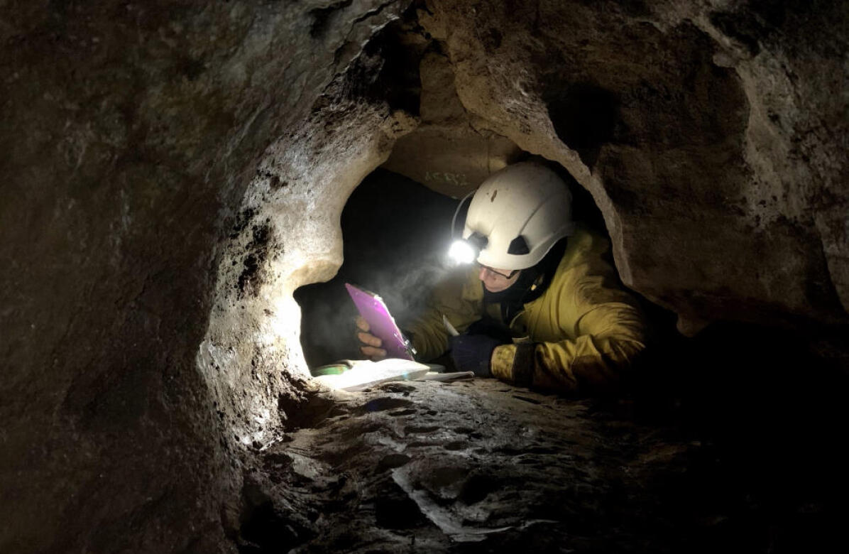
Traditional cave surveying is challenging because surveyors remain motionless for extended periods of time and are exposed to water, cool air, and rock, which can lead to hypothermia [2]. A more serious danger is getting lost or trapped in a cave [3] because specialized training is required to extract a physically incapacitated caver. The Barbara Schomer Cave Preserve in Clarion County, PA, has a cave that is particularly challenging to survey for two reasons: (1) the small size of the passages (typical natural passages are $0.75\text{\,}\mathrm{m}$ high and $0.75\text{\,}\mathrm{m}$ wide), and (2) the mazelike nature of the passages that are estimated to be $60\text{\,}\mathrm{km}$ in length [4, p. 10]. 50 cave surveyors have been involved in 30 trips to survey a total of $2522\text{\,}\mathrm{m}$ of passage (B. Ashbrook, personal communication, March 1, 2020). Each trip is 4-5 hours in duration and there are currently over 90 unexplored leads in the cave. Fig. 2 illustrates an excerpt of the current working map of the cave and Fig. 3 illustrates a caver sketching for the cave survey.

Robotic operations in undeveloped subterranean environments are challenging due to limited or nonexistent communication infrastructure that increases the risk of failure from data dropouts. Dang et al. [5] find that autonomy is necessary when operating underground because reliable high-bandwidth wifi connections are impossible to maintain after making turns. Low-frequency radio is commonly used in subterranean environments because it penetrates rock better than high-frequency radios (e.g., walkie-talkies) [6], but the disadvantage is that radio has low-bandwidth and data dropouts increase as range increases. Given these constraints, cave surveying robots must be autonomous to robustly operate in the presence of communication dropouts and must also represent the environment in a way that is both high-resolution yet compact so that data can be transmitted over low-bandwidth connections to operators. The ability to transmit high-resolution maps is desirable because human operators can direct exploration towards a particular lead of interest if the robot enters a passageway with multiple outgoing leads.

Figure 2: An excerpt of the current working map for the cave on the Barbara Schomer Cave Preserve in Clarion County, PA. The map is encoded with terrain features. Note the passages marked too tight for human access in the top-right of the image. Aerial robots could be deployed to these areas to collect survey data. Image courtesy of B. Ashbrook.

Figure 3: A caver sketches a passageway to produce content for the map shown in Fig. 2. Image courtesy of H. Wodzenski. J. Jahn pictured.

GMMs are ideal for perceptual modeling in the cave survey context because they represent depth information compactly. This paper seeks to address the problem of robotic exploration under constrained communication by proposing an autonomous system that leverages these compact perceptual models to transmit high-resolution information about the robot’s surroundings over low-bandwidth connections. Depth sensor observations are encoded as GMMs and used to maintain a consistent local occupancy grid map. A motion planner selects smooth and continuous trajectories that greedily maximize an information-theoretic objective function.

This work presents an extended version of prior work [7] introducing all contributions:

1. a method for real-time occupancy reconstruction from GMMs with LiDAR sensor observations,

2. an information-theoretic exploration system that leverages the occupancy modeling technique, and

3. evaluation of the exploration system in simulation and real-world experiments.

This manuscript presents the following additional contributions:

1. an extension of the real-time occupancy reconstruction from GMMs that can accomodate limited field of view depth cameras,

2. a motion planning framework that performs well for both LiDAR and limited field of view depth cameras, and

3. extensive evaluation of the exploration system in simulation and on hardware in a show cave in Pennsylvania and a wild cave in West Virginia.

The paper is organized as follows: Section II surveys related work, Sections III, LABEL:, IV, LABEL: and V describe the methodology, Section VI presents the experimental design and results, Section VII details the limitations of the approach, and Section VIII concludes with a discussion of future work.

II Related Work

State-of-the-art robotic technologies fail to provide rapid autonomy and persistent situational awareness that meet the operational challenges of subterranean environments [8]. The DARPA Subterranean Challenge [9] was created to foster the development of rapid autonomous missions through enhanced situational awareness to overcome the degraded environmental conditions, severe communication constraints, and expansive nature that are characteristic of subterranean regimes. As a result, several works have been developed pursuant to mine and urban autonomy and exploration. Section II-A provides an overview of the state of the art in subterranean autonomy. Section II-B reviews recent cave mapping works and Section II-C details works in occupancy modeling for exploration.

II-A Exploration in Subterranean Environments

A significant challenge in cave surveying is the ability to access leads and passageways that may be unreachable to humans as shown in Fig. 2. If the lead contains a passageway with several outgoing leads, it is useful for an operator to have the ability to direct exploration in one direction over others (e.g., one passageway is larger than another or contains more interesting features).  Murphy et al. [10] find that semiautonomy in the form of autonomous navigation coupled with human-assisted perception is preferred over total autonomy for robots operating in subterranean domains given that teleoperation was required to recover the autonomous $700\text{\,}\mathrm{kg}$ ATV-type Groundhog vehicle when it became stuck in a mine. However, human-assisted perception is predicated on the ability to transfer perceptual information to human operators. Baker et al. [11] develop Groundhog to collect data via teleoperation and build a map in postprocessing with the approach of [12]. Baker et al. [13] extend the capabilities of the Groundhog robot by developing a sense, plan, act cycle to autonomously map an abandoned mine that takes 90 seconds due to limited onboard processing.

Ebadi et al. [14] develop an architecture for LiDAR-based multi-robot SLAM that removes outlier loop closures via Incremental Consistent Measurement (ICM) Set Maximization and enables input from multiple sources and a human operator. The approach relies on VLP-16 Puck Lite LiDARs, which are relatively heavy and necessitate using ground vehicles as compared to the small aerial systems used in this work. The approach is tested in a mine that has relatively flat floors as compared to the highly uneven nature of the cave passages explored in this work. A limitation expressed in the work is the need for a compressed map representation to overcome the communication bottlenecks when transmitting visualizations to the user.

Dang et al. [15] demonstrate exploration in mine environments that employs a global planner when the local planner is unable to identify paths that increase information gain. The aerial system is large to accomodate the heavy LiDAR sensor which is appropriate for mine environments built for easy traverse by people but is too large for the tight crawlways of caves.

II-B Cave Mapping

Few works consider methods to map caves with aerial or ground robotic systems. Kaul et al. [16] develop the Bentwing robot to produce maps of cave environments. The approach, which requires a pilot to remotely operate the vehicle, may be challenging due to the cognitive load required to stabilize attitude and position simultaneously. The Bentwing uses a rotating 2D laser scanner to collect data that is postprocessed into a globally consistent map. Similarly, Tabib and Michael [17] develop a simultaneous localization and mapping strategy that represents sensor observations using GMMs and produces maps via postprocessing from data collected from an aerial system equipped with a 3D LiDAR. In contrast, this work produces a map in real-time onboard the autonomous robot, which is suitable for information-theoretic planning and sufficiently compact to be transmitted to operators over low-bandwidth connections for use in human-assisted perception.

The DEep Phreatic THermal eXplorer (DEPTHX) vehicle was developed to explore and characterize the biology of the Sistema Zacatón cenotes, or underwater sinkholes, in Tamaulipas, Mexico, as an analog mission for the search for life underneath Europa’s ice [18]. The probe combines LiDAR to map above the water table with sonar to map phreatic zones. The authors employ a Deferred Reference Octree data structure to represent the environment and mitigate the memory required to represent the underlying evidence grid. The cost of transmitting data to enable information sharing with human operators is not considered.

II-C Occupancy Modeling for Exploration

While many exploration approaches have leveraged voxel-based occupancy modeling strategies for information-theoretic planning [19], the large memory demands of using occupancy grid maps remains. Octomap [20] leverages an octree data structure to represent the environment at multiple resolutions and stores a probability of occupancy in each cell. A challenge of using octree structures for dynamically growing maps is that the time complexity of an access or query is $\mathcal{O}(\log n)$ [21]. Voxblox [21] represents the environment using a Truncated Signed Distance Field (TSDF) and employs voxel hashing, which yields $\mathcal{O}(1)$ look-up and insertion times, but suffers from the same discretization challenges as the occupancy grid map. The Normal Distribution Transform Occupancy Map (NDT-OM) attempts to mitigate the large memory demands of occupancy grid maps [22] by encoding a Gaussian density into occupied voxels based on the heuristic that larger voxels are sufficient to represent the environment at the same fidelity as a traditional occupancy grid map. However, this technique suffers from the same drawbacks as the occupancy grid map for exploration in large environments.

To overcome this limitation, this work builds upon prior work by O’Meadhra et al. [23] that compactly represents sensor observations as GMMs for the purpose of occupancy reconstruction by developing real-time local occupancy mapping for information-theoretic planning using both $360\text{\,}\mathrm{\SIUnitSymbolDegree}$ and limited FoV sensor models. Because sensor observations are stored as GMMs, local occupancy maps are constructed as needed and only GMMs need to be transmitted between the robot and operator, which results in a much smaller memory footprint. Another advantage is that occupancy grid maps of variable resolution could be used to plan paths at various resolutions (though this is not demonstrated in this work).

While GMMs have been used for compact perceptual modeling [24], occupancy modeling [23], and multi-robot exploration [25], these works do not demonstrate real-time operation. Our prior work [7] addresses this gap in the state of the art by proposing an exploration system that leverages GMMs for real-time 3D information theoretic planning and perceptual modeling using a $360\text{\,}\mathrm{\SIUnitSymbolDegree}$ field of view (FoV) sensor on computationally constrained platforms. The choice of sensor field of view (FoV) has implications for mapping, planning, and hardware design so this paper extends the prior work by considering both $360\text{\,}\mathrm{\SIUnitSymbolDegree}$ and limited FoV depth sensors.

III Overview

Figure 4: Overview of the autonomous exploration system presented in this work. Using pose estimates from a visual-inertial navigation system (Section VI-C1) and depth camera observations, the mapping method (Section IV-A and Section IV-B) builds a memory-efficient approximate continuous belief representation of the environment while creating local occupancy grid maps in real-time. A motion primitives-based information-theoretic planner (Section V) uses this local occupancy map to generate snap-continuous forward-arc motion primitive trajectories that maximize the information gain over time.

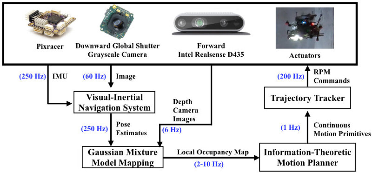
The exploration system consists of mapping, information-theoretic planning, and a monocular visual-inertial navigation system (Fig. 4). A brief review of GMMs is detailed in Section IV-A. Section IV-B develops the GMM-based local occupancy grid mapping strategy used by the planning approach to generate continuous trajectories that maximize an information-theoretic objective (Section V).

IV Mapping

IV-A Gaussian Mixture Models for Perception

(a) Color Image

(b) Depth Image

(c) PointCloud

(d) Free Space Windows

(e) GMM

(f) Resampled Data

Figure 5: Overview of the approach to transform a sensor observation into free and occupied GMMs. LABEL:sub@sfig:color_image A color image taken onboard the robot exploring Laurel Caverns. LABEL:sub@sfig:depth_image A depth image corresponding to the same view as the color image with distance shown as a heatmap on the right hand side (in meters). LABEL:sub@sfig:cave_pointcloud illustrates the point cloud representation of the depth image. LABEL:sub@sfig:cave_occ_free In the mapping approach, points at a distance smaller than a user-specified max range $r_{d}$ (in this case $r_{d}=$5\text{\,}\mathrm{m}$$) are considered to be occupied, and a GMM is learned using the approach detailed in Section IV-A1. Points at a distance further than $r_{d}$ are considered free, normalized to a unit vector, and projected to $r_{d}$. The free space points are projected to image space and windowed using the technique detailed in Section IV-A2 to decrease computation time. Each window is shown in a different color. LABEL:sub@sfig:cave_gmms The GMM representing the occupied-space points is shown in red and the GMM representing the free space points is shown in black. Sampling $2\times 10^{5}$ points from the distribution yields the result shown in LABEL:sub@sfig:cave_gmms_resampled. The number of points to resample is selected for illustration purposes and to highlight that the resampling process yields a map reconstruction with an arbitrary number of points.

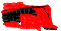
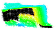
The approach leverages GMMs to compactly encode sensor observations for transmission over low-bandwidth communications channels. The GMM provides a generative model of sensor observations from which occupancy may be reconstructed by resampling from the distribution and raytracing through a local occupancy grid map. Formally, the GMM is a weighted sum of $M$ Gaussian probability density functions (PDFs). The probability density of the GMM is expressed as

$$p(\boldsymbol{x}|{\boldsymbol{\Theta}}) =\sum\limits_{m=1}^{M}\pi_{m}\mathcal{N}(\boldsymbol{x}|{\boldsymbol{\mu}}_{m},{\boldsymbol{\Lambda}}_{m})$$

where $p(\boldsymbol{x}|{\boldsymbol{\Theta}})$ is the probability density for the D-dimensional random variable $\boldsymbol{x}$ and is parameterized by ${\boldsymbol{\Theta}}=\{\pi_{m},{\boldsymbol{\mu}}_{m},{\boldsymbol{\Lambda}}_{m}\}_{m=1}^{M}$. $\pi_{m}\in\mathbb{R}$ is a weight such that $\sum_{m=1}^{M}\pi_{m}=1$ and $0\leq\pi_{m}\leq 1$, ${\boldsymbol{\mu}}_{m}$ is a mean, and ${\boldsymbol{\Lambda}}_{m}$ is a covariance matrix for the $m^{th}$ $D$-dimensional Gaussian probability density function of the distribution. The multivariate probability density for $\boldsymbol{x}$ is written as

$$\mathcal{N}(\boldsymbol{x}|{\boldsymbol{\mu}}_{i},{\boldsymbol{\Lambda}}_{i}) =\frac{|{\boldsymbol{\Lambda}}_{i}|^{-1/2}}{(2\pi)^{D/2}}\exp\Big{(}-\frac{1}{2}(\boldsymbol{x}-{\boldsymbol{\mu}}_{i})^{T}{\boldsymbol{\Lambda}}_{i}^{-1}(\boldsymbol{x}-{\boldsymbol{\mu}}_{i})\Big{)}.$$

In this work, a depth observation taken at time $t$ and consisting of $N$ points, $\mathcal{Z}_{t}=\{\boldsymbol{z}_{t}^{1},\ldots,\boldsymbol{z}_{t}^{n},\ldots,\boldsymbol{z}_{t}^{N}\}$, is used to learn a GMM. Estimating optimal GMM parameters ${\boldsymbol{\Theta}}$ remains an open area of research [26]. This work utilizes the Expectation Maximization (EM) algorithm to solve the maximum-likelihood parameter estimation problem, which is guaranteed to find a local maximum of the log likelihood function [27]. To make the optimization tractable, EM introduces latent variables $\mathbf{C}=\{c_{nm}\}$ for each point $\boldsymbol{z}_{t}^{n}$ and cluster $m$ and iteratively performs two steps: expectation (E) and maximization (M) [27, 28, 29].

The E step calculates the expected value of the complete-data log-likelihood $\ln p(\mathcal{Z}_{t},\mathbf{C}|{\boldsymbol{\Theta}})$ with respect to the unknown variables $\mathbf{C}$ given the observed data $\mathcal{Z}_{t}$ and current parameter estimates ${\boldsymbol{\Theta}}^{i}$, which is written as $E[\ln p(\mathcal{Z}_{t},\mathbf{C}|{\boldsymbol{\Theta}})|\mathcal{Z}_{t},{\boldsymbol{\Theta}}^{i}]$ [28]. This amounts to evaluating the posterior probability, $\beta_{nm}$, using the current parameter values ${\boldsymbol{\Theta}}^{i}$ (shown in  Eq. 1) [27]

$$\beta_{nm}=\frac{\pi_{m}\mathcal{N}(\boldsymbol{z}_{t}^{n}|{\boldsymbol{\mu}}_{m}^{i},{\boldsymbol{\Lambda}}_{m}^{i})}{\sum\limits_{j=1}^{M}\pi_{j}\mathcal{N}(\boldsymbol{z}_{t}^{n}|{\boldsymbol{\mu}}_{j}^{i},{\boldsymbol{\Lambda}}_{j}^{i})},$$ (1)

where $\beta_{nm}$ denotes the responsibility that component $m$ takes for point $\boldsymbol{z}_{t}^{n}$. The M step maximizes the expected log-likelihood using the current responsibilities, $\beta_{nm}$, to obtain updated parameters, ${\boldsymbol{\Theta}}^{i+1}$ via the following:

$${\boldsymbol{\mu}}_{m}^{i+1} =\sum_{n=1}^{N}\frac{\beta_{nm}\boldsymbol{z}_{t}^{n}}{\sum_{n=1}^{N}\beta_{nm}}$$ (2)

$${\boldsymbol{\Lambda}}_{m}^{i+1} =\sum\limits_{n=1}^{N}\frac{\beta_{nm}(\boldsymbol{z}_{t}^{n}-{\boldsymbol{\mu}}_{m}^{i+1})(\boldsymbol{z}_{t}^{n}-{\boldsymbol{\mu}}_{m}^{i+1})^{T}}{\sum_{n=1}^{N}\beta_{nm}}$$ (3)

$$\pi_{m}^{i+1} =\frac{\sum_{n=1}^{N}\beta_{nm}\boldsymbol{x}_{n}}{\sum_{n=1}^{N}\beta_{nm}}.$$ (4)

Every iteration of EM is guaranteed to increase the log likelihood and iterations are performed until a local maximum of the log likelihood is achieved [27].

The E step is computationally expensive because a responsibility $\beta_{nm}$ is calculated for each cluster $m$ and point $\boldsymbol{z}_{t}^{n}$, which amounts to $NM$ responsibility calculations. In the M step, every parameter must be updated by iterating over all $N$ samples in the dataset. In practice, a responsibility matrix $\mathbf{B}\in\mathbb{R}^{N\times M}$ is maintained whose entries consist of the $\beta_{nm}$ to estimate the parameters ${\boldsymbol{\Theta}}$.

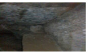
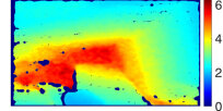
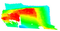
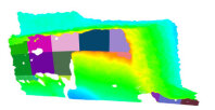
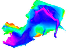
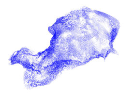
Following the work of O’Meadhra et al. [23], distinct occupied $\mathcal{G}(\boldsymbol{x})$ (detailed in Section IV-A1) and free $\mathcal{F}(\boldsymbol{x})$ (detailed in Section IV-A2) GMMs are learned to compactly represent the density of points observed in the environment (Fig. 5). The process by which $\mathcal{F}(\boldsymbol{x})$ and $\mathcal{G}(\boldsymbol{x})$ are created is illustrated in Figs. 5c and 5d. Because the GMM is a generative model, one may sample from the distribution (Fig. 5f) to generate points associated with the surface model and reconstruct occupancy (detailed in Section IV-B).

IV-A1 Occupied Space

For points with norms less than a user-specified maximum range $r_{d}$, the EM approach is adapted from [17] to accept points that lie within a Mahalanobis distance of $\lambda$. Because Gaussians fall off quickly, points far away from a given density will have a small effect on the updated parameters for that density. By reducing the number of points, this decreases the computational cost of the EM calculation. Only points that have a value smaller than $\lambda$ are considered (i.e., points larger than $\lambda$ are discarded):

$$\lambda>\sqrt{(\boldsymbol{x}_{n}-\boldsymbol{\mu}_{m}^{1})^{T}(\boldsymbol{\Lambda_{m}}^{1})^{-1}(\boldsymbol{x}_{n}-\boldsymbol{\mu}_{m}^{1})}$$ (5)

where the superscript 1 denotes the initialized values for the mean, covariance, and weight. This approach differs from our prior work Tabib et al. [7]; we utilize the approach in [17] as it yields greater frame-to-frame registration accuracy in practice. Frame-to-frame registration is not used in this work and is left as future work.

IV-A2 Free Space

To learn a free space distribution, points with norms that exceed the maximum range $r_{d}$ are projected to $r_{d}$. The EM approach from Section IV-A1 is used to decrease the computational cost of learning the distribution. To further reduce cost, the free space points are split into windows in image space and GMMs consisting of $n_{f}$ components are learned for each window. The windowing strategy is employed for learning distributions over free space points because it yields faster results and the distributions cannot be used for frame-to-frame registration. The number of windows and components per window is selected empirically.  Fig. 5d illustrates the effect of the windowing using colored patches and Fig. 5e illustrates the result of this windowing technique with black densities. Once the free space distributions are learned for each window the windowed distributions are merged into a single distribution.

Let $\mathcal{G}_{i}(\boldsymbol{x})$ be a GMM trained from $N_{i}$ points in window $i$ and let $\mathcal{G}_{j}(\boldsymbol{x})$ be a GMM trained from $N_{j}$ points in window $j$, where $\sum_{w=1}^{W}N_{w}=N$ for sensor observation $\mathcal{Z}_{t}$ and $W$ windows. $\mathcal{G}_{j}(\boldsymbol{x})=\sum_{k=1}^{K}\tau_{k}\mathcal{N}(\boldsymbol{x}|\boldsymbol{\nu}_{k},\boldsymbol{\Omega}_{k})$ may be merged into $\mathcal{G}_{i}(\boldsymbol{x})=\sum_{m=1}^{M}\pi_{m}\mathcal{N}(\boldsymbol{x}|\boldsymbol{\mu}_{m},\boldsymbol{\Lambda}_{m})$ by concatenating the means, covariances, and weights. However, care must be taken when merging the weights as they must be renormalized to sum to 1 [30]. The weights are renormalized via Eqs. 6 and 7:

$$N^{*} =N_{i}+N_{j}$$ (6)

$$\boldsymbol{\pi}^{*} =\begin{bmatrix}\frac{N_{i}\pi_{1}}{N^{*}}&\ldots&\frac{N_{i}\pi_{m}}{N^{*}}&\frac{N_{j}\tau_{1}}{N^{*}}&\ldots&\frac{N_{j}\tau_{k}}{N^{*}}\end{bmatrix}^{T}$$ (7)

where $m\in[1,\ldots,M]$ and $k\in[1,\ldots,K]$ denote the mixture component in GMMs $\mathcal{G}_{i}(\boldsymbol{x})$ and $\mathcal{G}_{j}(\boldsymbol{x})$, respectively. $N^{*}\in\mathbb{R}$ is the sum of the support sizes of $\mathcal{G}_{i}(\boldsymbol{x})$ and $\mathcal{G}_{j}(\boldsymbol{x})$. $\boldsymbol{\pi}^{*}\in\mathbb{R}^{M+K}$ are the renormalized weights. The means and covariances are merged by concatenation.

(a)

(b)

(c)

(d)

Figure 6: Overview of the method by which occupancy is reconstructed. LABEL:sub@sfig:bbxa The blue bounding box $b_{t+1}$ is centered around $\mathbf{X}_{t+1}$ and red bounding box $b_{t}$ is centered at $\mathbf{X}_{t}$. LABEL:sub@sfig:bbxb illustrates the novel bounding boxes in solid magenta, teal, and yellow colors that represent the set difference $b_{t+1}\setminus b_{t}$. LABEL:sub@sfig:novelbbx1 Given a sensor origin shown as a triad, resampled pointcloud, and novel bounding box shown in yellow, each ray from an endpoint to the sensor origin is tested to determine if an intersection with the bounding box occurs. The endpoints of rays that intersect the bounding box are shown in red. LABEL:sub@sfig:novelbbx2 illustrates how the bounding box occupancy values are updated. Endpoints inside the yellow volume update cells with an occupied value. All other cells along the ray (shown in blue) are updated to be free.

IV-B Local Occupancy Grid Map

The occupancy grid map [31] is a probabilistic representation that discretizes 3D space into finitely many grid cells $\mathbf{m}=\{m_{1},...,m_{|\mathbf{m}|}\}$. Each cell is assumed to be independent and the probability of occupancy for an individual cell is denoted as $p(m_{i}|\mathbf{X}_{1:t},\mathcal{Z}_{1:t})$, where $\mathbf{X}_{1:t}$ represents all vehicle states up to and including time $t$ and $\mathcal{Z}_{1:t}$ represents the corresponding observations. Unobserved grid cells are assigned the uniform prior of 0.5 and the occupancy value of the grid cell $m_{i}$ at time $t$ is expressed using log odds notation for numerical stability.

$$l_{t,i}\triangleq\log\Bigg{(}\frac{p(m_{i}|\mathcal{Z}_{1:t},\mathbf{X}_{1:t})}{1-p(m_{i}|\mathcal{Z}_{1:t},\mathbf{X}_{1:t})}\Bigg{)}-l_{0}$$

When a new measurement $\mathcal{Z}_{t}$ is obtained, the occupancy value of cell $m_{i}$ is updated as

$$l_{t,i}\triangleq l_{t-1,i}+L(m_{i}|\mathcal{Z}_{t})$$

where $L(m_{i}|\mathcal{Z}_{t})$ denotes the inverse sensor model of the robot and $l_{0}$ is the prior of occupancy [31].

Instead of storing the occupancy grid map $\mathbf{m}$ that represents occupancy for the entire environment viewed since the start of exploration onboard the vehicle, a local occupancy grid map $\bar{\mathbf{m}}_{t}$ is maintained centered around the robot’s pose $\mathbf{X}_{t}$. The local occupancy grid map moves with the robot, so when regions of the environment are revisited, occupancy must be reconstructed from the surface models $\mathcal{G}(\boldsymbol{x})$ and $\mathcal{F}(\boldsymbol{x})$. To reconstruct occupancy at time $t+1$ given $\bar{\mathbf{m}}_{t}$, the set difference of the bounding boxes $b_{t}$ and $b_{t+1}$ for $\bar{\mathbf{m}}_{t}$ and $\bar{\mathbf{\mathbf{m}}}_{t+1}$, respectively, are used to compute at most three non-overlapping bounding boxes (see Figs. 6a and 6b for example). The intersection of the bounding boxes remains up-to-date, but the occupancy of the novel bounding boxes must be reconstructed using the surface models $\mathcal{G}(\boldsymbol{x})$ and $\mathcal{F}(\boldsymbol{x})$. Raytracing is an expensive operation [32], so time is saved by removing voxels at the intersection of $b_{t}$ and $b_{t+1}$ from consideration.

Figure 7: For limited FoV sensors, the FoV is approximated by the illustrated blue and red rectangular pyramids. These FoVs may also be represented as tetrahedra. To determine if a sensor position should be stored, the overlapping volume between the two approximated sensor FoVs is found.

The local occupancy grid map at time $t+1$, $\bar{\mathbf{m}}_{t+1}$, is initialized by copying the voxels in local grid $\bar{\mathbf{m}}_{t}$ at the intersection of $b_{t+1}$ and $b_{t}$. In practice, the time to copy the local occupancy grid map is very low (on the order of a few tens of milliseconds) as compared to the cost of raytracing through the grid. Not all Gaussian densities will affect the occupancy reconstruction so to identify the GMM components that intersect the bounding boxes a KDTree [33] stores the means of the densities. A radius equal to twice the sensor’s max range is used to identify the components that could affect the occupancy value of the cells in the bounding box. A ray-bounding box intersection algorithm [34] checks for intersections between the bounding box and the ray from the sensor origin to the density mean. Densities that intersect the bounding box are extracted into local submaps $\bar{\mathcal{G}}(\boldsymbol{x})$ and $\bar{\mathcal{F}}(\boldsymbol{x})$. Points are sampled from each distribution and raytraced to their corresponding sensor origin to update the local grid map (example shown in Figs. 6c and 6d).

As the number of mixture components increases over time in one region, updating the occupancy becomes increasingly expensive as the number of points needed to resample and raytrace increases. The next sections detail how to limit the potentially unbounded number of points depending on the employed sensor model.

IV-C $360\text{\,}\mathrm{\SIUnitSymbolDegree}$ FoV Sensor Model

A small, fixed-size bounding box around the current pose with half-lengths $h_{x}$, $h_{y}$, and $h_{z}$ is used to determine if a prior observation was made within the confines of the bounding box. This bounding box approach works for sensors that have a 360^∘ field of view such as the 3D LiDAR used in this work, but does not readily extend to depth sensors with smaller fields of view (discussed in the next section). If a prior observation was made within the bounding box of the current observation, $\mathcal{Z}_{t}$ is not stored as a GMM. This has the effect of limiting the number of components that are stored over time.

IV-D Limited FoV Sensor Model

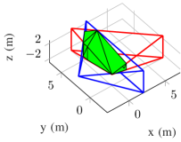
The limited FoV sensor model is directional, so it is approximated by two non-intersecting tetrahedra such that their union forms a rectangular pyramid (shown in Fig. 7). For two sensor FoVs the intersection between the four pairs of tetrahedra is calculated and the intersection points found. The convex hull of the intersection points is converted to a polyhedron mesh with triangular facets. The convex hull volume is found by summing individual volumes of the tetrahedra that make up the polyhedron [35]. The overlap is estimated as a percentage of overlapping volume between the two sensor FoVs and a sensor observation is only stored if its overlap exceeds a user-defined threshold. In this way, the number of components that represent a given location can be reduced while ensuring that the environment is covered.

V Planning for Exploration

(a)

(b)

(c)

Figure 8: Action space design for the proposed information-theoretic planner. LABEL:sub@subfig:single_mpl shows a single motion primitive library generated using bounds on the linear velocity along $\{{\mathbf{x}}_{\cal{B}},{\mathbf{z}}_{\cal{B}}\}$ and the angular velocity along $\{{\mathbf{z}}_{\cal{B}}\}$. LABEL:sub@subfig:prims_lidar and LABEL:sub@subfig:prims_tof show top-down views of the motion primitive library collections used when the sensor model is a LiDAR [7] and a depth camera [36] respectively (off-plane primitives are not shown). The proposed planner can be used with either of these sensors using the appropriate action space designs explained in Section V-A.

A motion planner designed for exploration of a priori unknown and unstructured spaces with an aerial robot must satisfy three requirements: (1) reduce entropy of the unknown map, (2) maintain collision-free operation, and (3) return motion plans in real-time. Several previous works provide information-theoretic frameworks towards meeting these objectives [37, 19, 38]. Julian et al. [37] use the Shannon mutual information between the map and potential sensor observations as a reward function to generate motion plans for exploration; however, computational requirements limit the number of potential trajectories over which the reward can be calculated. In contrast, the Cauchy-Schwarz Quadratic mutual information (CSQMI) has been demonstrated for real-time exploration with aerial robots [19, 7]. This work utilizes an information-theoretic planning strategy using CSQMI as the primary reward function, extending our prior work [7] to support limited FoV sensors in addition to $360$\mathrm{\SIUnitSymbolDegree}$$ FoV sensors. The proposed framework can be divided into two stages: (1) action space generation and (2) action selection. At the start of any planning iteration, the planner uses the action generation strategy (detailed in Section V-A) to generate a set of candidate actions up to a user-specified planning horizon using motion primitives. The action selector evaluates the collision-free and dynamically feasible subset of the action space using CSQMI as a reward function, returning the most informative plan to execute during the next planning iteration (see Sections V-B, LABEL: and V-C).

V-A Action Space Generation

This section describes: (1) background on the trajectory representation using motion primitive generation [39], and (2) the design of the action space.

V-A1 Forward-Arc Motion Primitive

Accurate position control of multirotors presumes continuity in the supplied tracking references up to high-order derivatives of position [40]. To represent a candidate trajectory, this paper utilizes sequential forward-arc motion primitives [39]. We use an extension to this work that ensures differentiability up to jerk and continuity up to snap [41]. Given the multirotor state at a time $t$, $\boldsymbol{\xi}_{t}=[x,y,z,\theta]^{\top}$, linear velocities in the body frame $[v_{{\mathbf{x}}_{\cal{B}}},v_{{\mathbf{z}}_{\cal{B}}}]$, and the angular velocity about ${\mathbf{z}}_{\cal{B}}$ axis, $\omega_{{\mathbf{z}}_{\cal{B}}}$, the forward-arc motion primitive is computed as a polynomial function of time generated using the following high-order constraints:

$$\dot{\boldsymbol{\xi}}_{\tau} =[v_{{\mathbf{x}}_{\cal{B}}}\cos{\theta},v_{{\mathbf{x}}_{\cal{B}}}\sin{\theta},v_{{\mathbf{z}}_{\cal{B}}},\omega_{{\mathbf{z}}_{\cal{B}}}]$$ (8)

$${\boldsymbol{\xi}}^{(n)}_{\tau} =\mathbf{0}\text{ for }n=2,3,4$$

where $\{.\}^{(n)}$ denotes the $n^{\text{th}}$ time derivative, and $\tau$ is the specified duration of the motion primitive. Motion primitives in the ${\mathbf{y}}_{\cal{B}}$ direction can also be obtained by replacing $v_{{\mathbf{x}}_{\cal{B}}}$ by $v_{{\mathbf{y}}_{\cal{B}}}$ in the above constraints. Later, we will use a combination of these directions to define the action space for the exploration planner that can operate with either a LiDAR or depth camera.

V-A2 Motion Primitive Library (MPL)

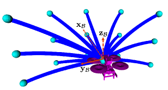
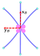
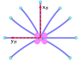
A motion primitive library (MPL) is a collection of forward-arc motion primitives generated using a user-specified discretization of the robot’s linear and angular velocities [39]. Let $\textbf{a}=\{v_{{\mathbf{x}}_{\cal{B}}},v_{{\mathbf{y}}_{\cal{B}}},v_{{\mathbf{z}}_{\cal{B}}},\omega_{{\mathbf{z}}_{\cal{B}}}\}$ be an action set that is generated with user-specified maximum velocity bounds in the ${\mathbf{x}}_{\cal{B}}-{\mathbf{y}}_{\cal{B}}$ plane and the ${\mathbf{z}}_{\cal{B}}$ direction. The motion primitive library is then given by the set (Fig. 8a):

$$\Gamma_{\boldsymbol{\xi}_{t}}=\{\gamma_{\boldsymbol{\xi}_{t}}(\textbf{a}_{jk},\tau)\mid\|[v_{\mathbf{x}},v_{\mathbf{y}}]\|\leq V_{\max},\|v_{\mathbf{z}}\|\leq V_{{\mathbf{z}}},\|\omega\|\leq\Omega\}$$ (9)

where $j\in[1,N_{\omega}]$ and $k\in[1,N_{{\mathbf{z}}}]$ define the action discretization for one particular primitive.

For each MPL, an additional MPL containing stopping trajectories at any state $\boldsymbol{\xi}_{t}$ can be generated by fixing the desired end point velocity to zero, $\dot{\boldsymbol{\xi}}_{\tau}=0$. These stopping trajectories are scheduled one planning round away from the starting time of the planning round. These trajectories help ensure safety in case the planner fails to compute an optimal action.

V-A3 Designing the Action Space

The final action space, $\mathcal{X}_{\text{act}}$, is a collection of MPLs selected according to three criteria: (1) information gain rate, (2) safety, and (3) compute limitations. Prior work [7] provides such a design for a $360$\mathrm{\SIUnitSymbolDegree}$$ FoV sensor (LiDAR). Goel et al. [36] present an analysis on how these three factors influence $\mathcal{X}_{\text{act}}$ for a limited FoV depth sensor. This work extends [7] using the analysis in [36], yielding a motion planner amenable for exploration with either a LiDAR or a depth sensor and that ensures similar exploration performance in either case (see Section VI).

Action Space for $360$\mathrm{\SIUnitSymbolDegree}$$ FoV Sensors

$360$\mathrm{\SIUnitSymbolDegree}$$ FoV sensors are advantageous in an exploration scenario for three reasons: (1) $360$\mathrm{\SIUnitSymbolDegree}$$ depth data from the sensor allows for visibility in all azimuthal directions, (2) a larger volume is explored per unit range when compared to a limited FoV sensor, and (3) yaw in-place motion does not help gain information. (1) enables backward and sideways motion in the action space $\mathcal{X}_{\text{act}}$ without sacrificing safety (Fig. 8b). (2) influences the entropy reduction: for the same trajectory, a sensor with a larger FoV will explore more voxels compared to the limited FoV case. (3) reduces the number of motion primitive libraries in the action space to yield increased planning frequency. An example of an action space designed while considering these factors is presented in [7] and the corresponding parameters are shown in Table Ia.

These factors indicate that the same action space $\mathcal{X}_{\text{act}}$ cannot be used for limited FoV cameras if comparable exploration performance is to be maintained. This motivates the need for an alternate and informed action design for the limited FoV cameras.

MPL ID	Vel., Time	$N_{\omega}$, $N_{\mathbf{z}}$	$N_{\text{prim}}$
$1$	$v_{{\mathbf{x}}_{\cal{B}}},\tau$	$3$, $5$	$15$
$2$	$v_{{\mathbf{x}}_{\cal{B}}},2\tau$	$3$, $5$	$15$
$3$	$-v_{{\mathbf{x}}_{\cal{B}}},\tau$	$3$, $5$	$15$
$4$	$-v_{{\mathbf{x}}_{\cal{B}}},2\tau$	$3$, $5$	$15$

(a) LiDAR

MPL ID	Vel., Time	$N_{\omega}$, $N_{\mathbf{z}}$	$N_{\text{prim}}$
$1$	$v_{{\mathbf{x}}_{\cal{B}}},\tau$	$3$, $5$	$15$
$2$	$v_{{\mathbf{x}}_{\cal{B}}},2\tau$	$3$, $5$	$15$
$3$	$v_{{\mathbf{y}}_{\cal{B}}},\tau$	$3$, $5$	$15$
$4$	$v_{{\mathbf{y}}_{\cal{B}}},2\tau$	$3$, $5$	$15$
$5$	$-v_{{\mathbf{y}}_{\cal{B}}},\tau$	$3$, $5$	$15$
$6$	$-v_{{\mathbf{y}}_{\cal{B}}},2\tau$	$3$, $5$	$15$
$7$	$\omega_{{\mathbf{z}}_{\cal{B}}},\tau$	$1$, $5$	$5$

(b) Depth Camera

TABLE I: Discretization used to construct the action space $\mathcal{X}_{\text{act}}$ for the simulation experiments for LABEL:sub@stab:lidar LiDAR and LABEL:sub@stab:tof depth camera cases. Total number of primitives for a MPL are denoted by $N_{\text{prim}}=N_{\omega}\cdot N_{\mathbf{z}}$. The base duration $\tau$ was kept at $3\text{\,}\mathrm{s}$ for all experiments.

Action Space for Limited FoV Sensors

Goel et al. [36] show that for an exploration planner using a limited FoV sensor, the design of the action space $\mathcal{X}_{\text{act}}$ can be informed by the sensor model. The authors consider a depth sensor to design $\mathcal{X}_{\text{act}}$ by incorporating the sensor range and FoV, among other factors. This work follows a similar approach yielding an action space that contains MPLs in both the ${\mathbf{x}}_{\cal{B}}$ and ${\mathbf{y}}_{\cal{B}}$ directions (Fig. 8c). The parameters to construct the MPL collection comprising $\mathcal{X}_{\text{act}}$ are shown in Table Ib. Note that there is an additional MPL corresponding to a yaw-in-place motion, unlike the $360$\mathrm{\SIUnitSymbolDegree}$$ FoV case, to compensate for the limited FoV of the depth camera. For further detail on how to obtain these parameters, please refer to [36, 42].

V-B Information-Theoretic Objective

The action selection policy uses CSQMI as the information-theoretic objective to maximize the information gain over time. CSQMI is computed at $k$ points along the primitive $\gamma_{\boldsymbol{\xi}_{t}}$, and the sum is used as a metric to measure the expected local information gain for a candidate action ${\cal{I}_{\gamma}}$. However, this design may result in myopic decision-making.

() (a) (b) (c) (c) (d) (e) (f) (g)

Figure 9: Exploration statistics for simulation experiments. The first row of results pertains to the LiDAR sensor model and the second row to the depth camera sensor model. LABEL:sub@sfig:6a and LABEL:sub@sfig:6d illustrate the map entropy over time for 160 trials (80 trials per sensor model and 40 trials per mapping method), LABEL:sub@sfig:6b and LABEL:sub@sfig:6e illustrate the average map entropy over time for each method. Although both methods achieve similar entropy reduction, MCG uses significantly less memory according to the average cumulative data transferred shown in LABEL:sub@sfig:6c and LABEL:sub@sfig:6f. When the LiDAR sensor model is used, the average cumulative data transferred at the end of $1500\text{\,}\mathrm{s}$ is $1.3\text{\,}\mathrm{MB}$ for the MCG approach and $256\text{\,}\mathrm{MB}$ for the OG approach. When the depth camera sensor model is used, the average cumulative data transferred at the end of $1500\text{\,}\mathrm{s}$ is $4.4\text{\,}\mathrm{MB}$ for the MCG approach and $153\text{\,}\mathrm{MB}$ for the OG approach. The MCG method represents a decrease of approximately one to two orders of magnitude as compared to the OG method for the LiDAR and depth camera sensor models, respectively. The experiments are conducted in the simulated cave environment shown in Fig. 9g. The four starting positions are shown as orange dots.

(a) Simulated Cave Environment

(a)

(b) GMM map (1$\sigma$ covariances)

(c) Resampled pointcloud

(d) Dense voxel map

(e) Points from the PLY

(e)

(f) GMM map (1$\sigma$ covariances)

(g) Resampled pointcloud

(h) Dense voxel map

Figure 10: The colorized mesh used in simulation experiments is shown in LABEL:sub@sfig:10a and produced from FARO scans of a cave in West Virginia. After $1500\text{\,}\mathrm{s}$ of exploration with a LiDAR sensor model, the resulting LABEL:sub@sfig:gmm_map_lidar MCG map is shown with 1$\sigma$ covariances and densely resampled with $1\text{\times}{10}^{6}\text{\,}$ points to obtain the reconstruction shown in LABEL:sub@sfig:resampled_lidar. LABEL:sub@sfig:dense_voxel_lidar illustrates the dense voxel map produced after a $1500\text{\,}\mathrm{s}$ trial with $20\text{\,}\mathrm{cm}$ voxels. LABEL:sub@sfig:10e illustrates the pointcloud from the mesh shown in LABEL:sub@sfig:10a. LABEL:sub@sfig:gmm_map_tof illustrates the MCG map with 1$\sigma$ covariances, which is densely resampled with $1\text{\times}{10}^{6}\text{\,}$ points, to obtain the reconstruction shown in LABEL:sub@sfig:resampled_tof. LABEL:sub@sfig:dense_voxel_tof illustrates the dense voxel map with $20\text{\,}\mathrm{cm}$ voxels after $1500\text{\,}\mathrm{s}$ of exploration with the depth camera sensor model. The reconstruction accuracy for LABEL:sub@sfig:resampled_lidar, LABEL:sub@sfig:dense_voxel_lidar, LABEL:sub@sfig:resampled_tof, and LABEL:sub@sfig:dense_voxel_tof are shown in Table II. All pointclouds shown are colored from red to purple according to z-height.

Therefore, frontiers are also incorporated to model the global spatial distribution of information [43]. This global reward, denoted by ${\cal{V}_{\gamma}}$, is calculated based on the change in distance towards a frontier along a candidate action. Using the node state $\boldsymbol{\xi}_{0}$, end point state $\boldsymbol{\xi}_{\tau}$, and a distance field constructed based on the position of the frontiers, this reward can be calculated as ${\cal{V}_{\gamma}}=d(\boldsymbol{\xi}_{0})-d(\boldsymbol{\xi}_{\tau})$, where $d(\boldsymbol{\xi}_{t})$ denotes the distance to the nearest voxel in the distance field from state $\boldsymbol{\xi}_{t}$ [25].

Algorithm 1 Overview of Action Selection for Exploration

1:input: $\mathcal{X}_{\text{act}}$, $\mathcal{X}_{\text{free}}$

2:output: $\gamma^{*}_{\boldsymbol{\xi}_{t}}$ $\triangleright$ best action

3:for $\Gamma_{\boldsymbol{\xi}_{t}}\in\mathcal{X}_{\text{act}}$ do

4:    for $\gamma_{\boldsymbol{\xi}_{t}}\in\Gamma_{\boldsymbol{\xi}_{t}}$ do

5:         feasible $\leftarrow$ SafetyCheck($\gamma_{\boldsymbol{\xi}_{t}}$, $\gamma^{\text{stop}}_{\boldsymbol{\xi}_{t}}$, $\mathcal{X}_{\text{free}}$)

6:         if feasible then

7:             ${\cal{I}_{\gamma}}\leftarrow$ InformationReward($\gamma_{\boldsymbol{\xi}_{t}}$)

8:             ${\cal{V}_{\gamma}}\leftarrow$ FrontierDistanceReward($\gamma_{\boldsymbol{\xi}_{t}}$)

9:         else

10:             ${\cal{I}_{\gamma}}\leftarrow 0.0$, ${\cal{V}_{\gamma}}\leftarrow 0.0$              

11:return $\gamma^{*}_{\boldsymbol{\xi}_{t}}\leftarrow\operatorname*{arg\,max}\limits_{\gamma_{\boldsymbol{\xi}_{t}}\in\mathcal{X}_{\text{act}}}[{\cal{I}_{\gamma}}+{\cal{V}_{\gamma}}]$

V-C Action Selection

Using the rewards described in the preceding section, the objective for the motion planner is defined as follows [36, 25]:

$$\begin{split}\operatorname*{arg\,max}\limits_{\gamma_{\boldsymbol{\xi}_{t}}}\leavevmode\nobreak\ &{\cal{I}_{\gamma}}+\alpha\,{\cal{V}_{\gamma}}\\ \mbox{s.t.}\leavevmode\nobreak\ &\gamma_{\boldsymbol{\xi}_{t}}\in\mathcal{X}_{\text{act}}\end{split}$$ (10)

where $\alpha$ is a weight that adjusts the contribution of the frontier distance reward. Recall, the goal is to maximize this reward function in real-time on a compute-constrained aerial platform. Previous information-theoretic approaches that construct a tree and use a finite-horizon planner either do not use a global heuristic [44] or are not known to be amenable for operation on compute-constrained platforms [25]. In this work, a single-step planner is used with the action space $\mathcal{X}_{\text{act}}$ consisting of motion primitives of varying duration for real-time performance (see Table I). Due to this choice, the planner computes rewards over candidate actions that extend further into the explored map from the current position. In this manner, longer duration candidate actions provide a longer lookahead than the case when all candidate actions are of the same duration, even in single-step planning formulations (see Table I).

The action selection procedure is detailed in Algorithm 1. For every candidate action $\gamma_{\boldsymbol{\xi}_{t}}$ in the action space $\mathcal{X}_{\text{act}}$, a safety check procedure is performed to ensure that this candidate and the associated stopping action ($\gamma^{\text{stop}}_{\boldsymbol{\xi}_{t}}$) are dynamically feasible and lie within free space $\mathcal{X}_{\text{free}}$ (5). The free space check is performed using a Euclidean distance field created from locations of occupied and unknown spaces in the robot’s local map given a fixed collision radius [45]. Checking that the stopping action is feasible ensures that the planner never visits an inevitable collision state, which is essential for safe operation [46]. If the action is feasible, the local information reward (${\cal{I}_{\gamma}}$, 7) and frontier distance reward (${\cal{V}_{\gamma}}$, 8) are determined as described in Section V-B. The planner then returns the action with the best overall reward (11).

Approach	LiDAR		Depth Camera
	Mean ($\text{\,}\mathrm{m}$)	Std ($\text{\,}\mathrm{m}$)	Mean ($\text{\,}\mathrm{m}$)	Std ($\text{\,}\mathrm{m}$)
MCG	$1.8\text{\times}{10}^{-02}\text{\,}$	$2.5\text{\times}{10}^{-02}\text{\,}$	$1.3\text{\times}{10}^{-02}\text{\,}$	$1.9\text{\times}{10}^{-02}\text{\,}$
OG	$6.2\text{\times}{10}^{-02}\text{\,}$	$3.9\text{\times}{10}^{-02}\text{\,}$	$6.3\text{\times}{10}^{-02}\text{\,}$	$3.9\text{\times}{10}^{-02}\text{\,}$

TABLE II: Reconstruction error for Fig. 10. The error is calculated as the PointCloud-to-Mesh distance between the environment reconstructions and mesh.

VI Experimental Design and Results

This section details the experimental design to validate the approach. Results are reported for both real-time simulation trials and field tests in caves. The following shorthand is introduced for this section only: MCG will refer to the Monte Carlo GMM mapping approach and OG mapping will refer to the Occupancy Grid mapping approach. The mapping and planning software is run on an embedded Gigabyte Brix 8550U with eight cores and $32\text{\,}\mathrm{GB}$ RAM, for both hardware and simulation experiments. Simulation results are presented for both LiDAR and depth camera sensor models, but hardware results are reported only for the depth camera case. Unless otherwise noted, the parameters for simulation and hardware experiments are equal.

VI-A Comparison Metrics

To calculate the memory requirements for the OG mapping approach, the incremental OG map is transmitted as a changeset pointcloud where each point consists of 4 floating point numbers: $\{x,y,z,\text{logodds}\}$. The changeset is computed after insertion of every pointcloud. A floating point number is assumed to be four bytes, or 32 bits. For the MCG approach, the cumulative data transferred is computed by summing the cost of transmitted GMMs. Each mixture component is transmitted as 10 floating point numbers: six numbers for the symmetric covariance matrix, three numbers for the mean, and one number for the mixture component weight. One additional number is stored per GMM that represents the number of points from which the GMM was learned. The transform between the sensor origin reference frame and the global reference frame is stored for each GMM using six numbers to represent the three translational and three rotational degrees of freedom. To ensure a fair comparison of exploration performance between the two approaches, a global occupancy grid serves as a referee and is maintained in the background with a voxel resolution of $0.2\text{\,}\mathrm{m}$. Exploration progress in simulation and hardware experiments is measured using the map entropy. The map entropy quantifies how the map’s uncertainty changes over time using the Shannon entropy of the global occupancy grid cells the robot could potentially observe [19, 47].

VI-B Simulation Experiments

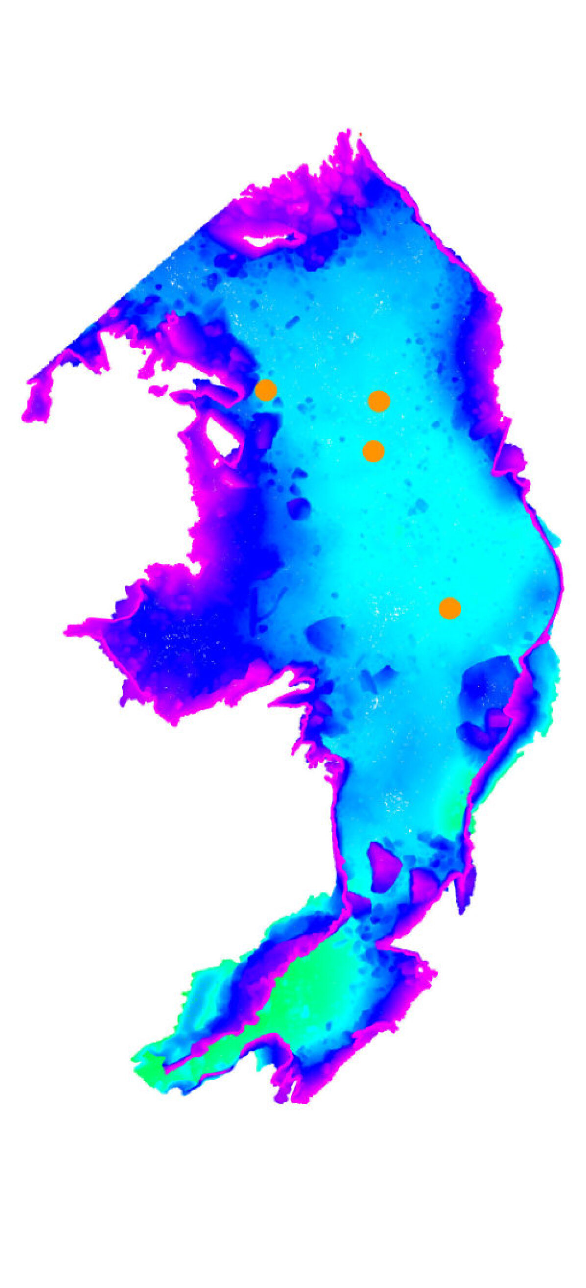
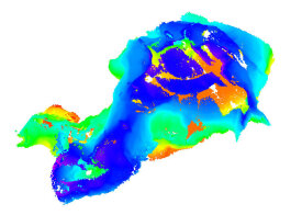
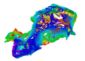
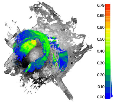
The exploration strategy is evaluated with 160 real-time simulation trials over approximately 67 hours in a $$30\text{\,}\mathrm{m}$\times$40\text{\,}\mathrm{m}$\times$6\text{\,}\mathrm{m}$$ environment constructed from colorized FARO pointclouds of a cave in West Virginia (see Fig. 9a). In each simulation, the multirotor robot begins exploration from one of four pre-determined starting positions and explores for $1500\text{\,}\mathrm{s}$. Ten exploration tests for each of the four sensor configurations are run from each of the four starting positions, leading to a total of 160 trials. The end time of $1500\text{\,}\mathrm{s}$ is empirically set based on the total time required to fully explore the cave. Note that ground truth state estimates are used for these simulation experiments, while the hardware experiments in Section VI-C rely on visual-inertial odometry (see Section VI-C1). The reconstruction error (Table II and Figs. 9c, 9d, 9g and 9h) is computed as pointcloud-to-mesh distances between reconstructed pointclouds from each trial and the environment mesh. In the case the MCG approach, the GMM map is densely resampled to produce a pointcloud. For the OG case, the occupancy grid map is converted to a pointcloud by assuming the points to be at the center of each voxel.

VI-B1 LiDAR Simulations

The LiDAR has a max range of $5.0\text{\,}\mathrm{m}$ and operates at $10\text{\,}\mathrm{Hz}$ for all simulation experiments. The motion planning parameters used in the action space design are shown in Table Ia. For all simulation trials, the maximum speed in the ${\mathbf{x}}_{\cal{B}}-{\mathbf{y}}_{\cal{B}}$ plane is $\|V_{\max}\|=$0.75\text{\,}\mathrm{m}\text{/}\mathrm{s}$$, the maximum speed along the ${\mathbf{z}}_{\cal{B}}$ axis is $V_{{\mathbf{z}}}=$0.5\text{\,}\mathrm{m}\text{/}\mathrm{s}$$, and the maximum yaw rate is $\Omega=$0.25\text{\,}\mathrm{rad}\text{/}\mathrm{s}$$. CSQMI is computed at the end point of the candidate action ($k=1$). $\lambda=5$ and $n_{f}=2$ for all simulations and hardware trials.

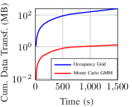
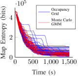
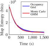
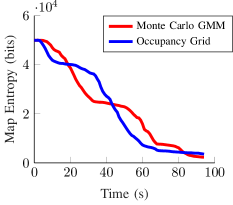
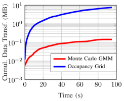
The simulation trials demonstrate that MCG achieves similar exploration performance as OG, which indicates that the approximations made by the former enables real-time performance without compromising exploration or map reconstruction quality (Figs. 9b and 9c). Figure 9c depicts the cumulative data that must be transferred to reproduce the OG and MCG maps remotely. After $1500\text{\,}\mathrm{s}$, transferring the MCG map requires $1.3\text{\,}\mathrm{MB}$ as compared to $256\text{\,}\mathrm{MB}$ to incrementally transfer the OG map. The MCG approach significantly outperforms the OG approach in terms of cumulative data transfer requirements. A representative example of the reconstructed GMM map for one trial from Fig. 9a is shown in Fig. 9b. Resampling $1\text{\times}{10}^{6}\text{\,}$ points from the distribution yields the map shown in Fig. 9c. The MCG approach has lower average reconstruction error as compared to the OG approach (Fig. 9d) as shown in Table II.

VI-B2 Depth Camera Simulations

The depth camera sensor model also has a max range of $5.0\text{\,}\mathrm{m}$ and operates at $10\text{\,}\mathrm{Hz}$ for all simulation experiments. A collection of motion primitive libraries used for the simulation experiments is shown in Table Ib. The velocity bounds for the simulation experiments are the same as in the LiDAR case.

(a)

(b)

(c)

(d)

(e)

(f)

(g)

(h)

Trial

Feasible Actions

Infeasible Actions

Planning

Occ. GMM

Free GMM

Occ. Recon.

Mean

Std.

Max.

Min.

Mean

Std.

Max.

Min.

Mean

Std.

Max.

Min.

Mean

Std.

Mean

Std.

Mean

Std.

(#)

(#)

(#)

(#)

(#)

(#)

(#)

(#)

($\text{\,}\mathrm{s}$)

($\text{\,}\mathrm{s}$)

($\text{\,}\mathrm{s}$)

($\text{\,}\mathrm{s}$)

($\text{\,}\mathrm{s}$)

($\text{\,}\mathrm{s}$)

($\text{\,}\mathrm{s}$)

($\text{\,}\mathrm{s}$)

($\text{\,}\mathrm{s}$)

($\text{\,}\mathrm{s}$)

0

$7.60\text{\,}$

$3.82\text{\,}$

$19\text{\,}$

$0\text{\,}$

$37.89\text{\,}$

$5.59\text{\,}$

$46\text{\,}$

$9\text{\,}$

$0.40\text{\,}$

$0.20\text{\,}$

$1.03\text{\,}$

$0.09\text{\,}$

$0.64\text{\,}$

$0.51\text{\,}$

$0.03\text{\,}$

$0.02\text{\,}$

$0.11\text{\,}$

$0.13\text{\,}$

1

$6.47\text{\,}$

$2.72\text{\,}$

$16\text{\,}$

$1\text{\,}$

$39.29\text{\,}$

$3.86\text{\,}$

$45\text{\,}$

$12\text{\,}$

$0.34\text{\,}$

$0.14\text{\,}$

$1.03\text{\,}$

$0.09\text{\,}$

$0.53\text{\,}$

$0.47\text{\,}$

$0.03\text{\,}$

$0.02\text{\,}$

$0.08\text{\,}$

$0.09\text{\,}$

2

$8.01\text{\,}$

$3.94\text{\,}$

$20\text{\,}$

$1\text{\,}$

$37.84\text{\,}$

$4.39\text{\,}$

$45\text{\,}$

$13\text{\,}$

$0.43\text{\,}$

$0.19\text{\,}$

$1.05\text{\,}$

$0.10\text{\,}$

$0.54\text{\,}$

$0.47\text{\,}$

$0.04\text{\,}$

$0.02\text{\,}$

$0.11\text{\,}$

$0.13\text{\,}$

3

$10.52\text{\,}$

$5.18\text{\,}$

$24\text{\,}$

$1\text{\,}$

$35.41\text{\,}$

$5.40\text{\,}$

$45\text{\,}$

$12\text{\,}$

$0.50\text{\,}$

$0.22\text{\,}$

$1.03\text{\,}$

$0.08\text{\,}$

$0.52\text{\,}$

$0.34\text{\,}$

$0.03\text{\,}$

$0.03\text{\,}$

$0.13\text{\,}$

$0.15\text{\,}$

4

$7.26\text{\,}$

$4.54\text{\,}$

$24\text{\,}$

$2\text{\,}$

$38.38\text{\,}$

$5.98\text{\,}$

$44\text{\,}$

$3\text{\,}$

$0.38\text{\,}$

$0.22\text{\,}$

$1.05\text{\,}$

$0.12\text{\,}$

$0.48\text{\,}$

$0.25\text{\,}$

$0.03\text{\,}$

$0.02\text{\,}$

$0.11\text{\,}$

$0.14\text{\,}$

(i) Planning and mapping statistics for the MCG trials in the flight arena

	Gigabyte Brix				Nvidia Jetson TX2
Trial	Autonomy		Realsense		VINS		BlueFox		PX4		Control		Comms
	CPU	Mem.	CPU	Mem.	CPU	Mem.	CPU	Mem.	CPU	Mem.	CPU	Mem.	CPU	Mem.
	(%)	($\mathrm{B}$)	(%)	($\mathrm{B}$)	(%)	($\mathrm{B}$)	(%)	($\mathrm{B}$)	(%)	($\mathrm{B}$)	(%)	($\mathrm{B}$)	(%)	($\mathrm{B}$)
0	186.52	$6.76\text{\times}{10}^{08}\text{\,}$	36.34	$1.29\text{\times}{10}^{08}\text{\,}$	154.84	$1.03\text{\times}{10}^{08}\text{\,}$	27.98	$8.50\text{\times}{10}^{07}\text{\,}$	16.98	$2.16\text{\times}{10}^{07}\text{\,}$	16.10	$3.15\text{\times}{10}^{07}\text{\,}$	0.19	$2.10\text{\times}{10}^{07}\text{\,}$
1	153.16	$7.76\text{\times}{10}^{08}\text{\,}$	30.43	$1.32\text{\times}{10}^{08}\text{\,}$	155.15	$1.05\text{\times}{10}^{08}\text{\,}$	27.82	$8.37\text{\times}{10}^{07}\text{\,}$	16.92	$2.14\text{\times}{10}^{07}\text{\,}$	15.96	$3.12\text{\times}{10}^{07}\text{\,}$	0.18	$1.91\text{\times}{10}^{07}\text{\,}$
2	182.52	$6.33\text{\times}{10}^{08}\text{\,}$	31.69	$1.33\text{\times}{10}^{08}\text{\,}$	153.76	$1.02\text{\times}{10}^{08}\text{\,}$	27.86	$8.55\text{\times}{10}^{07}\text{\,}$	16.88	$2.15\text{\times}{10}^{07}\text{\,}$	16.04	$2.91\text{\times}{10}^{07}\text{\,}$	0.19	$1.91\text{\times}{10}^{07}\text{\,}$
3	203.55	$7.61\text{\times}{10}^{08}\text{\,}$	29.58	$1.24\text{\times}{10}^{08}\text{\,}$	154.45	$1.01\text{\times}{10}^{08}\text{\,}$	27.85	$8.59\text{\times}{10}^{07}\text{\,}$	16.87	$2.14\text{\times}{10}^{07}\text{\,}$	15.99	$3.12\text{\times}{10}^{07}\text{\,}$	0.19	$2.10\text{\times}{10}^{07}\text{\,}$
4	178.78	$6.13\text{\times}{10}^{08}\text{\,}$	30.24	$1.31\text{\times}{10}^{08}\text{\,}$	151.46	$1.03\text{\times}{10}^{08}\text{\,}$	27.46	$8.56\text{\times}{10}^{07}\text{\,}$	16.88	$1.93\text{\times}{10}^{07}\text{\,}$	16.02	$2.91\text{\times}{10}^{07}\text{\,}$	0.20	$2.10\text{\times}{10}^{07}\text{\,}$

(j) Memory and compute statistics for the MCG trials in the flight arena

Figure 11: Results of repeatability trials for the MCG and OG approaches in a flight arena. LABEL:sub@sfig:fa_all_entropy illustrates the entropy reduction for five trials for the MCG and OG methods. LABEL:sub@sfig:fa_mean_entropy plots the standard error on top of the mean line. The cumulative data transferred is provided for each approach in LABEL:sub@sfig:fa_all_comms with the mean and standard deviation for the trials shown in LABEL:sub@sfig:fa_mean_comms. The theoretical (Th. OG and Th. MCG) communications is compared to actual (Ac. OG and Ac. MCG) communications transmitted to the base station using UDP. LABEL:sub@sfig:fa_flying_robot is a still image of the robot flying during one of the MCG trials (full video of the trial may be found at https://youtu.be/egwjv7YwHPE) and LABEL:sub@sfig:fa_reconstructed_map illustrates the live map transmitted to the base station from the same trial. LABEL:sub@sfig:planning_times provides a plot of the number of feasible actions in red with the planning time shown in blue.  LABEL:sub@sfig:octomap_comparison Uses data from the MCG flights and generates an Octomap in postprocessing to compare the communications required. The Octomap performance is similar to that of the OG approach. More details about this analysis is provided in Section VI-C3. LABEL:sub@tab:fa_planning and LABEL:sub@tab:fa_mem_compute provide timing, compute, and memory statistics for each subsystem for each of the five MCG flights. The figures reported in Fig. 11j are averages.

(a)

(b)

(c)

(d)

Figure 12: Results of forcing a communication dropout on the system. The aerial system is carried through a research lab and down a hallway away from the base station and router to force a communications dropout. The accompanying video may be found at https://youtu.be/UVn2BbMQRJg.  LABEL:sub@sfig:ghc_data_sent illustrates the data sent from the robot and LABEL:sub@sfig:ghc_data_rec is the data received by the base station (note: the base station and robot do not have their clocks synced). LABEL:sub@sfig:ghc_resulting_map illustrates the live map produced by the base station. LABEL:sub@sfig:ghc_helmet_cam illustrates a view of the aerial system at the start of the experiment from a camera mounted on the operator’s helmet.

(a)

(b)

(c)

(d)

(e)

(f)

(g)

Figure 13: LABEL:sub@sfig:rocky0803_explores A single aerial system explores the Dining Room of Laurel Caverns in Southwestern Pennsylvania. Still images of the robot exploring the environment are super-imposed to produce this figure. LABEL:sub@sfig:rocky0803 The aerial system with dimensions $$0.25\text{\,}\mathrm{m}$\times$0.41\text{\,}\mathrm{m}$\times$0.37\text{\,}\mathrm{m}$$ including propellers carries a forward-facing Intel Realsense D435 for mapping and downward-facing global shutter MV Bluefox2 camera (not shown). The pearl reflective markers are used for testing in a motion capture arena but are not used during field operations to obtain hardware results. Instead, a tightly-coupled visual-inertial odometry framework is used to estimate state during testing at Laurel Caverns. LABEL:sub@sfig:reconstruction_error illustrates the reconstruction error of the resampled GMM map as compared to the FARO map by calculating point-to-point distances. The distribution of distances is shown on the right-hand side. The mean error is $0.14\text{\,}\mathrm{m}$ with a standard deviation of $0.11\text{\,}\mathrm{m}$. In particular, there is misalignment in the roof due to pose estimation drift. LABEL:sub@sfig:figure11d A subset of the resampled GMM map (shown in black) is overlaid onto the FARO map (shown in colors ranging from red to purple) that displays the breakdown in the middle of the Dining Room. LABEL:sub@sfig:laurel_caverns_entropy The entropy reduction and LABEL:sub@sfig:laurel_caverns_comms cumulative data transferred for one trial for each of the Monte Carlo GMM mapping and OG mapping approaches are shown. The communication is a theoretical calculation – not actual transmitted data. While the map entropy reduction for each approach is approximately similar, the GMM mapping approach transmits significantly less memory than the OG mapping approach ($0.1\text{\,}\mathrm{MB}$ as compared to $7.5\text{\,}\mathrm{MB}$). LABEL:sub@sfig:laurel_caverns_rate illustrates the bit rate for each approach in a semi-logarithmic plot where the vertical axis is logarithmic. The black line illustrates how the approaches compare to 16kbps. For comparison, 16kbps is sufficient to transmit a low resolution (176 $\times$ 144 at 5 fps compressed to 3200 bit/frame) talking heads video [48, 49].

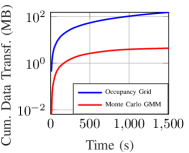
Similar to the LiDAR results, MCG outperforms OG in terms of memory efficiency while maintaining similar exploration performance. Figure 9f depicts the cumulative amount of data transfer in this case. After $1500\text{\,}\mathrm{s}$, transferring the MCG map requires $4.4\text{\,}\mathrm{MB}$ and $153\text{\,}\mathrm{MB}$ to incrementally transfer the OG map. Because the LiDAR has a larger field of view and lower resolution (i.e., fewer points for the same area of coverage) as compared to the depth camera, the LiDAR sensor model covers more voxels than a depth camera sensor model with the same voxel resolution. Rapid occupancy probability changes together with increasing field of view result in more affected voxels, which increases the amount of data that is transmitted. Voxel occupany probability is unclamped even if thresholds are exceeded. Similar to the LiDAR reconstruction, the MCG approach has lower average reconstruction error as compared to the OG approach (see Fig. 9h) as shown in Table II.

VI-C Hardware Experiments

VI-C1 Visual-Inertial Navigation and Control

State estimates are computed from IMU and downward-facing camera observations via VINS-Mono [50], a tightly-coupled visual-inertial odometry framework that jointly optimizes vehicle motion, feature locations, and IMU biases over a sliding window of monocular images and pre-integrated IMU measurements. The loop closure functionality of VINS-Mono is disabled to avoid having relocalization-induced discontinuities in the trajectory estimate, which would have significant implications for occupancy mapping and is left as future work.

For accurate trajectory tracking, a cascaded Proportional-Derivative (PD) controller is used with a nonlinear Luenberger observer to compensate for external acceleration and torque disturbances acting on the system [51]. To improve trajectory tracking, the controller uses angular feedforward velocity and acceleration terms computed from jerk and snap references computed from the reference trajectory’s $8^{\text{th}}$ order polynomial (Fig. 4).

Additionally, a state machine enables the user to trigger transitions between the following modes of flight operation: (1) takeoff, (2) hover, (3) tele-operation, (4) autonomous exploration, and (5) landing. The results presented in the next section all pertain to the autonomous exploration mode. In all of the trials included in this paper, the operator only intervenes to end the trial. For the full duration in all experiments, the robot operates completely autonomously.

VI-C2 Implementation Details

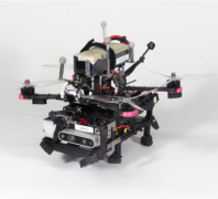
The exploration framework is deployed to the aerial system shown in Fig. 13b, a $2.5\text{\,}\mathrm{kg}$ platform equipped with a forward-facing Intel Realsense D435, downward-facing MV Bluefox2 camera, and downward and forward facing lights from Cree Xlamp XM-L2 High Power LEDs (Cool White 6500K). The MV Bluefox2 and D435 cameras operate at $60\text{\,}\mathrm{Hz}$ and output images of size $376\times 240$ and $848\times 480$, respectively. The MV Bluefox2 images are used in state estimation and the D435 depth images are throttled to $6\text{\,}\mathrm{Hz}$ for the the mapping system. The D435 camera estimates depth by stereo matching features in left- and right-infrared camera images augmented through a dot pattern projected by an IR projector. The laser power of the IR projector on the D435 is increased from a default value of $150\text{\,}\mathrm{mW}$ to $300\text{\,}\mathrm{mW}$ in order to improve observation quality in darkness.

The robot is equipped with an Auvidea J120 carrier board with NVIDIA TX2 and Gigabyte Brix 8550U that communicate over ethernet. The TX2 performs state estimation and control functions while the Brix performs mapping and planning. The flight controller used for all experiments is the Pixracer, but the platform is also equipped with a Betaflight controller as a secondary flight controller. Switching between the two controllers can be done via a switch on the RC transmitter. The drone frame is an Armattan Chameleon Ti LR 7” on which a Lumenier BLHeli_32 32bit 50A 4-in-1 electronic speed controller is mounted. The aerial system is a quadrotor that uses T-Motor F80 Pro 1900KV motors and DAL Cyclone 7056C propellers.

For all hardware experiments, $\|V_{\max}\|=$0.5\text{\,}\mathrm{m}\text{/}\mathrm{s}$$, $V_{{\mathbf{z}}}=$0.25\text{\,}\mathrm{m}\text{/}\mathrm{s}$$, and the motion primitives with duration $2\tau$ in Table Ib are disabled.

VI-C3 Flight Arena Experiments

Experiments were conducted in a flight arena with the aerial system. Each approach (MCG and OG) was flown five times for $150\text{\,}\mathrm{s}$. The results are shown in Fig. 11 and a video of one MCG trial with the live map displayed on the base station may be found at https://youtu.be/egwjv7YwHPE.

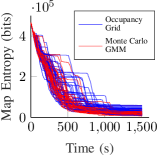
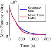
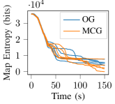
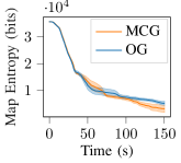
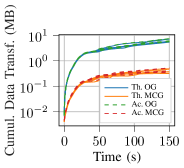
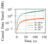
Figure 11a illustrates the map entropy over time for the 10 trials (5 for each approach) and Fig. 11b provides the mean and standard error for each trial. The communications plots shown in Fig. 11c and  Fig. 11d illustrate the theoretical cost to transmit the data (labeled as Th. OG and Th. MCG) that was calculated during the simulation trials (shown in Figs. 9c and 9f) as well as the actual transmitted data (labeled as Ac. OG and Ac. MCG in dashed lines). The actual transmitted data is calculated as the cumulative sum of the size of the UDP packets sent over the WiFi router to the base station. This plot demonstrates that the theoretical estimate closely matches the actual transmitted amount of data. No communications dropouts occurred in these trials because the base station and router were stationary and close to the aerial system’s flight volume.  Section VI-C4 analyzes the effect of the robot moving away from the base station and router to force a communications dropout.

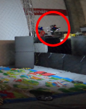
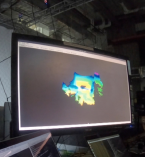
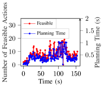
Figure 11e contains still images of the flight and Fig. 11f depicts a live map. Fig. 11g plots the number of feasible actions available to the robot at a given time on the left and the time to plan on the right.

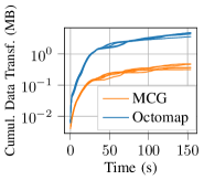
Figure 11h plots the theoretical data transferred and compares it to the OctoMap volumetric map [20]. To generate this plot, a $0.2\text{\,}\mathrm{m}$ leaf size OctoMap that matches the OG approach’s voxel size is created. For each scan added to the map, the set of voxels whose occupancy values (note: not state) have changed are used to generate an OctoMap submap (i.e., a new OctoMap that contains the change set). Submaps for this analysis are created by storing the incremental change set as an OctoMap to enable the exact map to be reconstructed on the receiving computer. The full probabilistic model is saved to disk because occupancy probabilities must be preserved to enable calculation of the mutual information [38] for information-theoretic exploration. The serialized stream does not contain any 3D coordinates. Instead, the spatial relationships between the nodes are stored in the encoding. Eight bits per node are used to specify whether a child node exists and an additional floating point number stores the occupancy value for that node. Due to this design there is some overhead to encode the multi-resolution nature of the data structure. The results demonstrate that the MCG approach also outperforms the OctoMap approach in terms of communication efficiency.

Figure 11i provides statistics for the planning and mapping components for the MCG trials. The planning times and statistics about the planning actions are provided. Out of all the trials, the planning subsystem triggers the stopping action only once (in Trial 0). Timing results for the generated occupied and free GMMs as well as the time to reconstruct occupancy are provided.

Figure 11j provides mean memory and compute statistics for the autonomy subsystem, which consists of mapping and planning. It also provides statistics for the Realsense, Bluefox, and PX4 subsystems to quantify the memory and CPU utilization to stream images and IMU measurements as well as transmitting cascaded commands to the flight controller. Statistics are also provided for communication and state estimation.

VI-C4 Communication Dropout Experiment

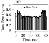
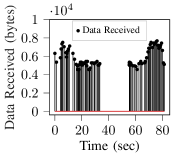
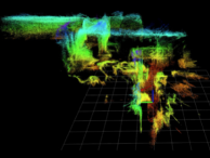
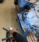
A communication dropout was triggered by performing an experiment where the aerial system is carried away from the WiFi router until it is out of range. Figures 12a and 12b depict the data sent from the aerial system and received by the base station over time (note: the clocks on the aerial system and base station are not synchronized). A view of the operating environment and map is shown in Fig. 12c. While data is dropped (i.e., the packets are lost due to the UDP communications protocol) at around $35\text{\,}\mathrm{s}$, the communications are re-established at around $55\text{\,}\mathrm{s}$ when the robot reapproaches the base station. A video at https://youtu.be/UVn2BbMQRJg illustrates the experiment.

(a)

(b)

(c) Image courtesy of C. Bassett

(d)

Figure 14: Overview of the results from experiments in a cave in West Virginia. LABEL:sub@sfig:rapps_hardware_entropy The map entropy over time for three trials of the MCG and OG approaches.  LABEL:sub@sfig:rapps_hardware_comms The data transferred between a robot and base station for each trial. The communication reported is actual transmitted data over UDP to a base station. Note that while the exploration performance is similar for both approaches, the data transferred for the MCG approach is substantially less.  LABEL:sub@sfig:rapps_cave1 A still image of the robot flying near a formation with terminated growth.  LABEL:sub@sfig:rapps_cave2 A composite image of one exploration trial composed of still images.

VI-C5 Laurel Caverns

The approach is tested in total darkness at Laurel Caverns, a commercially operated cave system in Southwestern Pennsylvania consisting of over four miles of passages.

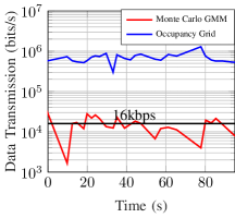
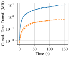
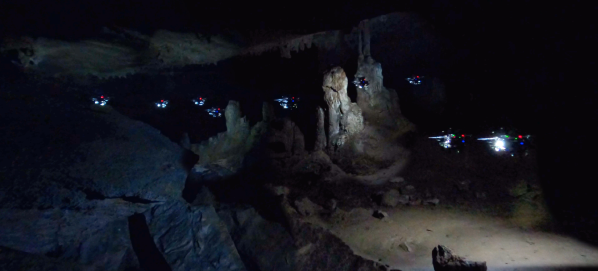
Figure 13a illustrates a composite image from several still images of the robot exploring the Laurel Caverns Dining Room. Two experiments were conducted, one for each of the MCG and OG approaches for a $95\text{\,}\mathrm{s}$ duration. The map entropy reduction over time is shown in Fig. 13e and is similar for both approaches, while the cumulative data transferred (Fig. 13f) to represent the maps is more than an order of magnitude lower for the MCG approach as compared to the OG approach. Note, however, that the communication reported for this experiment represents the theoretical, or estimated, communications needed to transmit the data. The data was not transmitted to a base station. The data transfer rate in Fig. 13g is calculated using Euler differentiation but note that the accuracy is affected by the limited number of samples. During hardware trials, a bounding box was used to constrain the exploration volume. To put the localization accuracy into perspective, the drift in position is about $0.53\text{\,}\mathrm{m}$ during a $50.9\text{\,}\mathrm{m}$ cave flight and the rotation drift is about $0.32\text{\,}\mathrm{rad}$ over $33.5\text{\,}\mathrm{rad}$ which is about a 1% drift in both translation and rotation. Position drift may be approximated as the difference between the initial and final position estimates because the robot takes off and lands at the same location.

VI-C6 West Virginia Cave

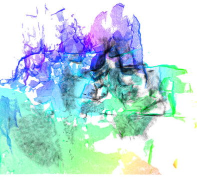
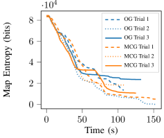
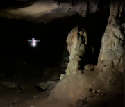
The approach was also tested in total darkness in a cave in West Virginia. Figure 14a illustrates the map entropy reduction over time with a maximum duration of $150\text{\,}\mathrm{s}$. The MCG and OG approaches perform similarly in these trials. The actual data transferred between the robot and base station is shown in Fig. 14b. Figure 14c is a still image of the robot approaching a formation and Fig. 14d is a composite image from several still images of the robot exploring the cave. A video of one exploration run may be found at the following link: https://youtu.be/H8MdtJ5VhyU. In these experiments a bounding box was used to constrain the exploration volume. The drift in position is about $1.28\text{\,}\mathrm{m}$ during the $82.6\text{\,}\mathrm{m}$ flight and rotation drift is about $0.55\text{\,}\mathrm{rad}$ over $41.8\text{\,}\mathrm{rad}$ which is about a 1.5% drift in position and 1.3% drift in rotation.

VII Discussion and Limitations

A limitation of the current work is that while the simulation assumes perfect state estimates, the VINS state estimator used onboard the aerial robot drifts over time. While it is not possible to entirely eliminate noise, some ways to mitigate the error are by (1) incorporating the depth observations from the forward-facing realsense camera into the VINS estimates and (2) incorporating loop closures.

Another limitation of the work is multiple representations are required to enable mapping, planning and state estimation. The map representation leverages GMMs, planning utilizes occupancy grid maps, and state estimation uses a sparse-point set.

Finally, there are many parameters that must be tuned in order for the system to function well. A potential source of future work is to automate this process.

VIII Conclusions and Future Work

The results presented in this paper comprise the beginning of a promising line of research for autonomous cave surveying and mapping by aerial systems. A high-fidelity model amenable to transmission across low-bandwidth communications channels is achieved by leveraging GMMs to compactly represent the environment. The method is demonstrated with $360\text{\,}\mathrm{\SIUnitSymbolDegree}$ and limited field of view sensors utilizing a planning framework that is amenable to both sensor models. Several avenues of future work remain. Cave maps are typically annotated with important terrain features such as stalactites, stalagmites, and breakdown (see Fig. 2 for example), but this work does not consider the problem of terrain feature classification and encoding. Additionally, waterproof, rugged, and easy-to-use 2D maps are critical for cave rescuers or explorers to avoid getting lost in caves. Methods to project the 3D map information from the robot to 2D are needed to fill this gap in the state of the art. Finally, the deployment of multiple robots to increase the speed of exploration is of interest for large passages or maze caves. Introducing re-localization strategies to curb drift over long duration flights and yield more consistent maps would also be beneficial for multi-robot operations. Beyond cave applications, this work has relevance for search and rescue, planetary exploration, and tactical operations where humans and robots must share information in real-time.

IX Acknowledgments

The authors thank C. Bassett for faciliating experiments at the West Virginia cave. The authors also thank H. Brooks and R. Maurer for facilitating experiments at Laurel Caverns and thank D. Cale for granting permission to test at Laurel Caverns. The authors also thank D. Melko for support and guidance regarding test sites, lending equipment and teaching the authors about caving. The authors thank B. Ashbrook for his insights and information regarding the cave on the Barbara Schomer Cave Preserve in Clarion County, PA. The authors thank H. Wodzenski and J. Jahn for providing images used in this work. Finally, the authors thank X. Yang for fruitful discussions about motion primitives-based planning and A. Dhawale, A. Desai, E. Cappo, T. Lee, M. Collins, and M. Corah for feedback on this manuscript.

Wennie Tabib received the B.S. degree in computer science in 2012, the M.S. degree in robotics in 2014, and the Ph.D. degree in computer science in 2019 from Carnegie Mellon University, Pittsburgh, PA, USA. She is currently a Systems Scientist with the Robotics Institute at Carnegie Mellon University. She researches perception, planning, and learning algorithms to enable safe autonomy in significantly three-dimensional, complex environments. Her current research develops methods to enable aerial systems to explore subterranean environments. Wennie is also a member of the National Speleological Society (NSS 69985), Mid-Atlantic Karst Conservancy, Pittsburgh Grotto and Loyalhanna Grotto.

Kshitij Goel received the B.Tech. degree in aerospace engineering in 2017 from the Indian Institute of Technology (IIT) Kharagpur, Kharagpur, WB, India. He is currently a Ph.D. student in Robotics at Carnegie Mellon University, researching fast motion planning for multirotors operating in unknown environments. His current work focuses on robustly deploying teams of multirotors to rapidly explore challenging real world scenarios in real time.

John Yao received the B.A.Sc. degree in aerospace engineering from the University of Toronto, Toronto, Canada, in 2013 and the M.S. degree in robotics from Carnegie Mellon University (CMU), Pittsburgh, PA, USA in 2016. John is a Ph.D. Candidate in the Robotics Institute at CMU. His research interests include visual-inertial state estimation and resource-constrained sensor fusion for autonomous robots.

Curtis Boirum received the B.S. degree in physical science from Eureka College, Eureka, IL, USA, in 2008. He received the B.S. and M.S. degrees in mechanical engineering from Bradley Unversity, Peoria, IL, USA, in 2009 and 2011, respectively. He received the M.S. degree in robotics from Carnegie Mellon University, Pittsburgh, PA, USA, in 2015. Curtis is a systems engineer for the Resilient Intelligent Systems Lab who designs, builds, and operates drones and ground robots ranging in size from 100g to 7kg.

Nathan Michael received the Ph.D. degree in mechanical engineering from the University of Pennsylvania, Philadelphia, PA, USA, in 2008. He is an Associate Research Professor in the Robotics Institute of Carnegie Mellon University; Director of the Resilient Intelligent Systems Lab; author of over 160 publications on control, perception, and cognition for resilient intelligent single and multi-robot systems; nominee or recipient of nine best paper awards; recipient of the Popular Mechanics Breakthrough Award and Robotics Society of Japan Best Paper Award (of 2014); PI of past and ongoing research programs supported by ARL, AFRL, DARPA, DOE, DTRA, NASA, NSF, ONR, and industry; and Chief Technical Officer of Shield AI. Nathan develops resilient intelligent autonomous systems capable of individual and collective intelligence through introspection, adaptation, and evolvement in challenging domains.

References

- Gunn [2004] J. Gunn, Encyclopedia of Caves and Karst Science. New York, NY: Taylor & Francis, 2004.
- Aulenbach et al. [2016] B. Aulenbach et al., Caving Basics: A Comprehensive Guide for Beginning Cavers, 4th ed. Huntsville, AL: National Speleological Society, 2016.
- Breisch [2011] R. L. Breisch, Lost in a Cave: Applying Graph Theory to Cave Exploration. Huntsville, AL: National Speleological Society, 2011.
- Frank [1985] E. F. Frank, Nittany Grotto News, vol. 32, no. 5, p. 10, 1985.
- Dang et al. [2019] T. Dang et al., “Field-hardened robotic autonomy for subterranean exploration,” in Conf. on Field and Service Robot., Tokyo, Japan, Aug. 2019.
- Gibson [2003] D. Gibson, “Channel characterisation and system design for sub-surface communications,” Ph.D. dissertation, University of Leeds, 2003.
- Tabib et al. [2019] W. Tabib, K. Goel, J. Yao, M. Dabhi, C. Boirum, and N. Michael, “Real-time information-theoretic exploration with gaussian mixture model maps,” in Proc. of Robot.: Sci. and Syst., FreiburgimBreisgau, Germany, June 2019.
- Tardioli et al. [2019] D. Tardioli, L. Riazuelo, D. Sicignano, C. Rizzo, F. Lera, J. L. Villarroel, and L. Montano, “Ground robotics in tunnels: Keys and lessons learned after 10 years of research and experiments,” Journal of Field Robotics, vol. 36, no. 6, pp. 1074–1101, 2019. [Online]. Available: https://onlinelibrary.wiley.com/doi/abs/10.1002/rob.21871
- Chung [2017] T. Chung. (2017) DARPA subterranean (SubT) challenge. https://www.darpa.mil/news-events/2017-12-21. DARPA Challenge TTO. Online: accessed 13 July 2020.
- Murphy et al. [2009] R. R. Murphy, J. Kravitz, S. L. Stover, and R. Shoureshi, “Mobile robots in mine rescue and recovery,” IEEE Robot. Autom. Mag., vol. 16, no. 2, pp. 91–103, 2009.
- Baker et al. [2006] C. Baker, Z. Omohundro, S. Thayer, W. Whittaker, M. Montemerlo, and S. Thrun, A Case Study in Robotic Mapping of Abandoned Mines. Berlin, Heidelberg: Springer Berlin Heidelberg, 2006, pp. 487–495. [Online]. Available: https://doi.org/10.1007/10991459_47
- Montemerlo et al. [2002] M. Montemerlo, D. Hahnel, D. Ferguson, R. Triebel, W. Burgard, S. Thayer, W. Whittaker, and S. Thrun, “A system for three-dimensional robotic mapping of undrground mines,” Carnegie Mellon University, Tech. Rep. CMU-CS-02-185, 2002.
- Baker et al. [2004] C. Baker, A. Morris, D. Ferguson, S. Thayer, C. Whittaker, Z. Omohundro, C. Reverte, W. Whittaker, D. Hahnel, and S. Thrun, “A campaign in autonomous mine mapping,” in Proc. of the IEEE Intl. Conf. on Robot. and Autom., vol. 2, April 2004, pp. 2004–2009 Vol.2.
- Ebadi et al. [2020] K. Ebadi, Y. Chang, M. Palieri, A. Stephens, A. Hatteland, E. Heiden, A. Thakur, N. Funabiki, B. Morrell, S. Wood, L. Carlone, and A.-a. Agha-mohammadi, “Lamp: Large-scale autonomous mapping and positioning for exploration of perceptually-degraded subterranean environments,” in Proc. of the IEEE Intl. Conf. on Robot. and Autom., 2020, pp. 80–86.
- Dang et al. [2019] T. Dang, F. Mascarich, S. Khattak, C. Papachristos, and K. Alexis, “Graph-based path planning for autonomous robotic exploration in subterranean environments,” in 2019 IEEE/RSJ International Conference on Intelligent Robots and Systems (IROS), 2019, pp. 3105–3112.
- Kaul et al. [2016] L. Kaul, R. Zlot, and M. Bosse, “Continuous-time three-dimensional mapping for micro aerial vehicles with a passively actuated rotating laser scanner,” J. Field Robot., vol. 33, no. 1, pp. 103–132, 2016.
- Tabib and Michael [2019] W. Tabib and N. Michael, “Simultaneous localization and mapping of subterranean voids with gaussian mixture models,” in Conf. on Field and Service Robot., Tokyo, Japan, Aug. 2019.
- [18] M. Gary, N. Fairfield, W. C. Stone, D. Wettergreen, G. Kantor, and J. M. Sharp, 3D Mapping and Characterization of Sistema Zacatón from DEPTHX.
- Charrow et al. [2015] B. Charrow, S. Liu, V. Kumar, and N. Michael, “Information-theoretic mapping using Cauchy-Schwarz quadratic mutual information,” in Proc. of the IEEE Intl. Conf. on Robot. and Autom., Seattle, WA, May 2015.
- Hornung et al. [2013] A. Hornung, K. M. Wurm, M. Bennewitz, C. Stachniss, and W. Burgard, “Octomap: An efficient probabilistic 3d mapping framework based on octrees,” Autonomous Robots, vol. 34, no. 3, pp. 189–206, 2013.
- Oleynikova et al. [2017] H. Oleynikova, Z. Taylor, M. Fehr, R. Siegwart, and J. Nieto, “Voxblox: Incremental 3d euclidean signed distance fields for on-board mav planning,” in Intelligent Robots and Systems (IROS), 2017 IEEE/RSJ International Conference on. IEEE, 2017, pp. 1366–1373.
- Saarinen et al. [2013] J. Saarinen, H. Andreasson, T. Stoyanov, J. Ala-Luhtala, and A. J. Lilienthal, “Normal distributions transform occupancy maps: Application to large-scale online 3d mapping,” in Proc. of the IEEE Intl. Conf. on Robot. and Autom. IEEE, 2013, pp. 2233–2238.
- O’Meadhra et al. [2019] C. O’Meadhra, W. Tabib, and N. Michael, “Variable resolution occupancy mapping using gaussian mixture models,” IEEE Robot. Autom. Letters, vol. 4, no. 2, pp. 2015–2022, April 2019.
- Srivastava and Michael [2019] S. Srivastava and N. Michael, “Efficient, multifidelity perceptual representations via hierarchical gaussian mixture models,” IEEE Trans. Robotics, vol. 35, no. 1, pp. 248–260, Feb 2019.
- Corah et al. [2019] M. Corah, C. O’Meadhra, K. Goel, and N. Michael, “Communication-efficient planning and mapping for multi-robot exploration in large environments,” IEEE Robotics and Automation Letters, vol. 4, no. 2, pp. 1715–1721, April 2019.
- Hosseini and Sra [2017] R. Hosseini and S. Sra, “An alternative to em for gaussian mixture models: Batch and stochastic riemannian optimization,” Mathematical Programming, pp. 1–37, 2017.
- Bishop [2007] C. Bishop, Pattern Recognition and Machine Learning. New York: Springer-Verlag New York, 2007.
- Bilmes et al. [1998] J. A. Bilmes et al., “A gentle tutorial of the em algorithm and its application to parameter estimation for gaussian mixture and hidden markov models,” Intl. Comput. Sci. Inst., vol. 4, no. 510, p. 126, 1998.
- Eckart et al. [2015] B. Eckart, K. Kim, A. Troccoli, A. Kelly, and J. Kautz, “Mlmd: Maximum likelihood mixture decoupling for fast and accurate point cloud registration,” in Intl. Conf. on 3D Vision. IEEE, 2015, pp. 241–249.
- Srivastava [2017] S. Srivastava, “Efficient, multi-fidelity perceptual representations via hierarchical gaussian mixture models,” Master’s thesis, Robotics Institute, Carnegie Mellon University, Pittsburgh PA, August 2017.
- Thrun et al. [2005] S. Thrun, W. Burgard, and D. Fox, Probabilistic robotics. MIT press, 2005.
- Amanatides et al. [1987] J. Amanatides, A. Woo et al., “A fast voxel traversal algorithm for ray tracing,” in Eurographics, vol. 87, no. 3, 1987, pp. 3–10.
- Blanco and Rai [2014] J. L. Blanco and P. K. Rai, “nanoflann: a C++ header-only fork of FLANN, a library for nearest neighbor (NN) with kd-trees,” https://github.com/jlblancoc/nanoflann, 2014.
- Williams et al. [2005] A. Williams, S. Barrus, R. K. Morley, and P. Shirley, “An efficient and robust ray-box intersection algorithm,” in ACM SIGGRAPH 2005 Courses. ACM, 2005, p. 9.
- [35] E. W. Weisstein, Tetrahedron. [Online]. Available: http://mathworld.wolfram.com/Tetrahedron.html
- Goel et al. [2019a] K. Goel, M. Corah, C. Boirum, and N. Michael, “Fast exploration using multirotors: Analysis, planning, and experimentation,” in Conf. on Field and Service Robot., Tokyo, Japan, Aug. 2019.
- Julian et al. [2014] B. J. Julian, S. Karaman, and D. Rus, “On mutual information-based control of range sensing robots for mapping applications,” J. Intl. & Robot. Research, vol. 33, no. 10, pp. 1357–1392, 2014.
- Zhang et al. [2019] Z. Zhang, T. Henderson, V. Sze, and S. Karaman, “Fsmi: Fast computation of shannon mutual information for information-theoretic mapping,” in 2019 International Conference on Robotics and Automation (ICRA), May 2019, pp. 6912–6918.
- Yang et al. [2017] X. Yang, K. Sreenath, and N. Michael, “A framework for efficient teleoperation via online adaptation,” in Proc. of the IEEE Intl. Conf. on Robot. and Autom. IEEE, 2017, pp. 5948–5953.
- Mellinger and Kumar [2011] D. Mellinger and V. Kumar, “Minimum snap trajectory generation and control for quadrotors,” in Proc. of the IEEE Intl. Conf. on Robot. and Autom., Shanghai, China, May 2011.
- Spitzer et al. [2018] A. Spitzer, X. Yang, J. Yao, A. Dhawale, K. Goel, M. Dabhi, M. Collins, C. Boirum, and N. Michael, “Fast and agile vision-based flight with teleoperation and collision avoidance on a multirotor,” in Proc. of the Intl. Sym. on Exp. Robot. Buenos Aires, Argentina: Springer, 2018, to be published.
- Goel et al. [2019b] K. Goel, M. Corah, and N. Michael, “Fast exploration using multirotors: Analysis, planning, and experimentation,” The Robotics Institute, Carnegie Mellon University, Tech. Rep. CMU-RI-TR-19-03, 2019.
- Yamauchi [1997] B. Yamauchi, “A frontier-based approach for autonomous exploration,” in Proc. of the Intl. Sym. on Comput. Intell. in Robot. and Autom., Monterey, CA, Jul. 1997.
- Tabib et al. [2016] W. Tabib, M. Corah, N. Michael, and R. Whittaker, “Computationally efficient information-theoretic exploration of pits and caves,” in Proc. of the IEEE/RSJ Intl. Conf. on Intell. Robots and Syst., Daejeon, Korea, Oct. 2016.
- Corah and Michael [2018] M. Corah and N. Michael, “Distributed matroid-constrained submodular maximization for multi-robot exploration: theory and practice,” Auton. Robots, 2018.
- Janson et al. [2018] L. Janson, T. Hu, and M. Pavone, “Safe motion planning in unknown environments: Optimality benchmarks and tractable policies,” in Proc. of Robot.: Sci. and Syst., Pittsburgh, PA, Jul. 2018.
- Cover and Thomas [2012] T. M. Cover and J. A. Thomas, Elements of information theory. John Wiley & Sons, 2012.
- Contin and Battista [1994] L. Contin and S. Battista, “Performance evaluation of video coding schemes working at very low bit rates,” in Proceedings of ICASSP ’94. IEEE International Conference on Acoustics, Speech and Signal Processing, vol. v, April 1994, pp. V/409–V/412 vol.5.
- Masry and Hemami [2001] M. Masry and S. S. Hemami, “An analysis of subjective quality in low bit rate video,” in Proceedings 2001 International Conference on Image Processing (Cat. No.01CH37205), vol. 1, Oct 2001, pp. 465–468 vol.1.
- Qin et al. [2018] T. Qin, P. Li, and S. Shen, “Vins-mono: A robust and versatile monocular visual-inertial state estimator,” IEEE Trans. Robotics, vol. 34, no. 4, pp. 1004–1020, August 2018.
- Michael et al. [2010] N. Michael, D. Mellinger, Q. Lindsey, and V. Kumar, “The grasp multiple micro-uav testbed,” in IEEE Robot. Autom. Mag., Sep. 2010.
- Patrick [2004] K. J. Patrick, Pennsylvania Caves and other Rocky Roadside Wonders. Stackpole Books, 2004.
- Bradley [2014] R. S. Bradley, Paleoclimatology: Reconstructing Climates of the Quaternary. Saint Louis: Elsevier Science & Technology, 2014, online: accessed 3 November 2020.
- Frick et al. [2010] W. F. Frick, J. F. Pollock, A. C. Hicks, K. E. Langwig, D. S. Reynolds, G. G. Turner, C. M. Butchkoski, and T. H. Kunz, “An emerging disease causes regional population collapse of a common north american bat species,” Science, vol. 329, no. 5992, pp. 679–682, 2010.
![[Uncaptioned image]](/html/2003.13883/assets/biography/wtabib.jpg) |