Efficient nonparametric inference on the effects of stochastic interventions under two-phase sampling, with applications to vaccine efficacy trials

Abstract

The advent and subsequent widespread availability of preventive vaccines has altered the course of public health over the past century. Despite this success, effective vaccines to prevent many high-burden diseases, including HIV, have been slow to develop. Vaccine development can be aided by the identification of immune response markers that serve as effective surrogates for clinically significant infection or disease endpoints. However, measuring immune response is often costly, which has motivated the usage of two-phase sampling for immune response sampling in clinical trials of preventive vaccines. In such trials, measurement of immunological markers is performed on a subset of trial participants, where enrollment in this second phase is potentially contingent on the observed study outcome and other participant-level information. We propose nonparametric methodology for efficiently estimating a counterfactual parameter that quantifies the impact of a given immune response marker on the subsequent probability of infection. Along the way, we fill in a theoretical gap pertaining to the asymptotic behavior of nonparametric efficient estimators in the context of two-phase sampling, including a multiple robustness property enjoyed by our estimators. Techniques for constructing confidence intervals and hypothesis tests are presented, and an open source software implementation of the methodology, the txshift R package, is introduced. We illustrate the proposed techniques using data from a recent preventive HIV vaccine efficacy trial.

1 Introduction

Ascertaining the population-level causal effects of exposures is often a motivating goal in scientific research. Such effects are commonly formulated via summaries of the distribution of counterfactual random variables, which describe the values a measurement would have taken if, possibly counter-to-fact, a particular level of exposure were assigned to the unit. Often, the exposure of interest is continuous-valued — for example, the dose of a drug, amount of weekly exercise, or level of an immune response marker induced by a vaccine. The latter serves as our motivating example as we consider data generated by a phase IIb trial of a vaccine to prevent infection by human immunodeficiency virus (HIV), the HIV Vaccine Trials Network’s (HVTN) 505 efficacy trial (Hammer et al., 2013). In addition to evaluating the overall efficacy of the vaccine, a key secondary question of the trial was to evaluate the role of vaccine-induced immune responses in generating protective efficacy against HIV (Janes et al., 2017). Identification of immune response markers causally related to protection is critical both for further developing a biological understanding of the action mechanism of a vaccine’s effects and for insights to guide the development of future vaccines.

To study such relationships, it is natural to consider a dose-response curve that summarizes participants’ risk of HIV infection as a function of the level of a particular immune response marker. A causal formulation of such a dose-response analysis would consider a (possibly infinite) collection of counterfactual outcomes, each representing the HIV infection risk that would have been observed if all individuals’ immune responses had been set to a particular level. Studying how the proportion of infected individuals varies as a function of the level of an immune response marker could provide insights into causal mechanisms underlying the vaccine’s effects. Unfortunately, several difficulties, both theoretical and practical, arise when considering such a dose-response approach. From a statistical perspective, nonparametric estimation and inference on the causal dose-response curve is challenging and requires non-standard techniques (Díaz and van der Laan, 2013; Kennedy et al., 2017; van der Laan et al., 2018). More importantly, such an approach may require consideration of counterfactual variables that are scientifically unrealistic. Namely, it may be impossible to imagine a world where every participant exhibits high immune responses, simply due to phenotypic variability of participants’ immune systems. This calls into question the validity of counterfactual dose-response analysis strategies that evaluate the effects of immune response markers.

An alternative framework for assessing the causal effects of continuous-valued exposures is rooted in considering counterfactual outcomes resulting from stochastic interventions (Díaz and van der Laan, 2012; Haneuse and Rotnitzky, 2013; VanderWeele and Hernan, 2013; Young et al., 2014). Whereas static interventions assign the same fixed level of an exposure to all observed units, stochastic interventions consider instead setting the exposure level equal to a random draw from a particular distribution. This approach provides a more flexible means of defining counterfactual random variables. Indeed, static interventions can be viewed as a special case of stochastic interventions in which the intervention mechanism is drawn from a degenerate distribution with all mass placed on only a single exposure level. In order to define scientifically meaningful counterfactuals, care must be taken in defining the particular distribution from which the exposure is drawn. A popular strategy is to draw exposure levels from a modified version of the true exposure distribution — the natural distribution of the exposure that occurs under no intervention. For example, one may consider an intervention that draws the post-vaccination level of immune response markers from a distribution that is similar to the naturally observed (post-vaccination) distribution of immune response markers but that has been shifted upwards (or downwards) for some or all participants. Counterfactuals defined by such an intervention may be better aligned with plausible future interventions, such as refinements of the current vaccine that provide improved immune response in some or all participants. Evaluating the population-level risk of HIV infection under such interventions is scientifically useful for several reasons. Firstly, this measure of risk provides a scientifically relevant mechanism by which to rank-order immune response markers by their importance for HIV infection risk. Such information could be used in defining go/no-go criteria in future early-phase HIV vaccine development pipelines. Secondly, the risk measure may also provide a way to predict next-generation vaccine efficacy based on the induced immune response profile, elucidating whether the immune response induced by a candidate vaccine is sufficiently promising to advance it to the clinical trials.

The above discussion highlights the need for rigorous methodology to identify and estimate population-level causal effects of stochastic interventions; recent work has provided several candidate approaches (Díaz and van der Laan, 2012; Haneuse and Rotnitzky, 2013; Young et al., 2014; Kennedy, 2019). Both Díaz and van der Laan (2012) and Haneuse and Rotnitzky (2013) propose conditions for the identification of the causal effect under a stochastic intervention and detail several estimators of these quantities, including strategies relying on inverse probability weighting, outcome regression, and doubly robust estimation. These approaches alone are insufficient for application to studies like the HVTN 505 trial, where a two-phased, case-control sampling design was used to measure participants’ immune response profiles. Under this design, all participants were HIV-negative at the week 24 visit, with eligible cases being vaccine recipients diagnosed with HIV-1 infection by the month 24 visit; 100% of cases were sampled from among those with samples available for measurement of immune response markers at the week 26 visit, while a random sample of eligible HIV-uninfected vaccine recipients was taken (Janes et al., 2017). This sampling design severely complicates the estimation of causal effects. Rose and van der Laan (2011), among others, discuss strategies for efficient estimation under two-phase sampling designs, emphasizing an inverse probability of censoring weighted modification that may be coupled with targeted minimum loss estimation (or similar frameworks) to account for study design. Their approach yields an asymptotically linear estimator so long as the probability of inclusion in the second-phase sample is known by design or estimable via nonparametric maximum likelihood. This latter requirement precludes usage of their proposed estimators in situations where, for example, sampling probabilities depend on continuous-valued covariates. While the term “two-phase sampling” has traditionally been used to denote outcome-dependent Bernoulli or without-replacement sampling based on discrete covariates, recent efforts have extended the concept to the usage of continuous-valued covariates in constructing second-phase samples (e.g., Chatterjee and Chen, 2007; Gilbert et al., 2014). Consequently, Rose and van der Laan (2011) sketched a more complicated procedure for generating efficient estimators in such settings. This approach has neither been evaluated via simulation nor in data analysis.

In the present work, we develop estimators of the mean counterfactual outcome under a stochastic intervention when the exposure is measured via two-phase sampling. We provide several contributions to the disparate literatures on two-phase sampling and stochastic interventions. To the former, we (i) formalize the assumptions needed for efficient nonparametric inference under two-phase sampling; (ii) characterize a multiple robustness of the estimators that arises from the second-order remainder of a linear expansion of the target parameter; and (iii) provide the first comparison of the practical performance of these estimators in rigorous numerical experiments. Our contributions to the literature on stochastic interventions are (i) a novel estimator of a conditional density that is valid under two-phase sampling, while achieving a fast convergence rate, a crucial development for generating efficient estimators of the mean counterfactual; and (ii) an extension of nonparametric inference on mean counterfactuals under stochastic interventions using projections onto nonparametric working marginal structural models. Finally, we provide open source software packages, txshift (Hejazi and Benkeser, 2020) and haldensify (Hejazi et al., 2020), for the R statistical programming environment (R Core Team, 2020), that facilitate implementation of our proposed estimators and their nuisance regression functions, respectively.

The remainder of this work is organized as follows. In Section 2, we introduce the target parameter (2.1) and discuss prior work on stochastic interventions (2.2) and two-phase sampling (2.3). Section 3 includes discussion of strategies for estimating nuisance regression functions (3.1) and the formulation of two estimators (3.2) that achieve the nonparametric efficiency bound for estimation of the counterfactual mean under a stochastic intervention. Numerical experiments comparing the proposed estimators to simpler variants are presented in section 4. Section 5 describes an analysis of data from the HVTN 505 trial using our proposed methodology. We conclude by summarizing the results of our statistical and scientific investigations and discussing avenues for future investigation.

2 Preliminaries and Background

2.1 Notation, data, and target parameter

Consider data generated by typical cohort sampling: the data on a single observational unit is denoted $X=(W,A,Y)$, where $W\in\mathcal{W}$ is a vector of baseline covariates, $A\in\mathcal{A}$ a real-valued exposure, and $Y\in\mathcal{Y}$ an outcome of interest. Initially, we assume access to $n$ independent copies of $X$, using $P_{0}^{X}$ to denote the distribution of $X$. We assume a nonparametric statistical model $\mathcal{M}^{X}$ for $P_{0}^{X}$. We denote by $q_{0,Y}$ the conditional density of $Y$ given $\{A,W\}$ with respect to some dominating measure, $q_{0,A}$ the conditional density of $A$ given $W$ with respect to dominating measure $\mu$, and $q_{0,W}$ the density of $W$ with respect to dominating measure $\nu$. We use $p_{0}^{X}$ to denote the density of $X$ with respect to the product measure. This density evaluated on a typical observation $x$ may be expressed

$$p_{0}^{X}(x)=q_{0,Y}(y\mid A=a,W=w)q_{0,A}(a\mid W=w)q_{0,W}(w)\ .$$

To define a counterfactual quantity of interest, we introduce a nonparametric structural equation model (NPSEM) to describe the data-generating process of $X$ (Pearl, 2000). Specifically, we assume the data are generated by the following system of structural equations:

$$W=f_{W}(U_{W});A=f_{A}(W,U_{A});Y=f_{Y}(A,W,U_{Y}),$$

where $\{f_{W},f_{A},f_{Y}\}$ are deterministic functions, and $\{U_{W},U_{A},U_{Y}\}$ are exogenous random variables.

The NPSEM provides a parameterization of $p_{0}^{X}$ in terms of the distribution of the random variables $(X,U)$ modeled by the system of structural equations. Importantly, it also implies a model for the distribution of counterfactual random variables generated by specific interventions on the data-generating process. For example, a static intervention replaces $f_{A}$ with a value $a$ in the support of $A$. By contrast, a stochastic intervention modifies the value $A$ would naturally assume, $f_{A}(W,U_{A})$, replacing it with a draw from a post-intervention distribution $\tilde{q}_{0,A}(\cdot\mid W)$, where the zero subscript is included to emphasize that this distribution may depend on $P_{0}^{X}$. A static intervention may be viewed as a particular type of stochastic intervention in which $\tilde{q}_{0,A}(\cdot\mid W)$ places all mass on a single point. Díaz and van der Laan (2012) described a stochastic intervention that draws $A$ from a distribution such that $\tilde{q}_{0,A}(a\mid W)=q_{0,A}(a-\delta(W)\mid W)$ for a user-supplied shifting function $\delta(W)$ and a given $a\in\mathcal{A}$. Haneuse and Rotnitzky (2013) showed that estimating the effect of this intervention is equivalent with that of an intervention that modifies the value $A$ would naturally assume according to a regime $d(A,W)$. Importantly, the regime $d(A,W)$ may depend on both the covariates $W$ and the exposure level $A$ that would be assigned in the absence of the regime; consequently, this has been termed a modified treatment policy (MTP). Both Haneuse and Rotnitzky (2013) and Díaz and van der Laan (2018) considered an MTP of the form $d(a,w)=a+\delta(w)$ for $\delta(w)=\gamma\in\mathbb{R}$ if $a+\gamma\leq u(w)$ and $d(a,w)=a$ if $a+\gamma>u(w)$, where $u(w)$ is the maximum value in the support of $q_{0,A}(\cdot\mid W=w)$. This intervention generates a counterfactual random variable $Y_{A+\delta(W)}\coloneqq f_{Y}(A+\delta(W),W,U_{Y})$ whose distribution we denote $P_{0}^{\delta}$; we seek to estimate $\psi_{0,\delta}\coloneqq\mathbb{E}_{P_{0}^{\delta}}\{Y_{A+\delta(W)}\}$, the mean of this counterfactual outcome.

In the context of the HVTN 505 trial, this parameter corresponds to the counterfactual risk of HIV-1 infection had the levels of immune response markers of vaccinated participants been increased by $\gamma$ units relative to the level induced by the current vaccine. This quantity may reflect the immune response marker distribution of a next-generation HIV vaccine with improved immunogenicity relative to the vaccine evaluated in HVTN 505. While the magnitude of shifting could generally be allowed to vary with participant characteristics, in our analysis, we consider an intervention that uniformly shifts all participants’ immune responses by $\gamma$ units, that is, $d(a,w)=a+\gamma$ for all $a\in\mathcal{A}$. Note that for HVTN 505, the parameter of interest is defined only for the vaccine group, making $A$ a post-vaccination marker measuring an HIV-specific immune response. Importantly, it is not conceivable to define the target parameter for placebo recipients since only HIV-negative participants are enrolled in the trial and $A$ is only defined if measured prior to HIV infection; consequently, all relevant placebo recipients have value zero for the marker $A$, and it is not meaningful to apply $d(a,w)$ to shift the distribution of $A$.

Analysis of the HVTN 505 trial is complicated by its two-phase sampling design, a technique commonly used for assessing vaccine-mediated immune response in efficacy trials (Haynes et al., 2012). In general two-phase sampling, we do not observe $X$ on all participants. Instead, we observe $O=(W,C,CA,Y)\sim P_{0}$, where $P_{0}$ is the distribution of $O$ and $C$ is an indicator that an observation is included in the second-phase sample. In particular, $C_{i}=1$ if $A$ is measured on the $i^{\text{th}}$ observation and $C_{i}=0$ otherwise. By convention, $CA$ denotes that unobserved values of $A$ are set to zero; this arbitrary labeling has no effect on our subsequent developments. In the context of vaccine trials, the probability of inclusion in the second-phase sample often depends on $W$ and $Y$; for each $w$ and $y$ we define $g_{0,C}(y,w)\coloneqq\mathbb{P}(C=1\mid Y=y,W=w)$. Consequently, $P_{0}\in\mathcal{M}=\{P_{P^{X}_{0},g_{0,C}}:P_{0}^{X}\in\mathcal{M}^{X},g_{0,C}\}$ — that is, $P_{0}$ is the distribution of $O$ implied by the pair $\{P^{X}_{0},g_{0,C}\}$. For example, in HVTN 505 all infected participants with samples available for marker measurement at week 28 had immune responses measured, i.e., $g_{0,C}(1,w)=1$ for all $w$; however, only a subset of non-infected participants had immune responses measured. We will assume access to an i.i.d. sample $O_{1},\ldots,O_{n}$, denoting its empirical distribution by $P_{n}$. The statistical estimation problem is thus to develop efficient nonparametric estimators of $\psi_{0,\delta}$ based on $n$ independent realizations of the observed data unit $O$.

2.2 Identifying the counterfactual mean under a stochastic intervention

Díaz and van der Laan (2012) established that $\psi_{0,\delta}$ is identified by

$$\psi_{0,\delta} =\int_{\mathcal{W}}\int_{\mathcal{A}}\overline{Q}_{0,Y}(a,w)q_{0,A}(a-\delta(W)\mid W=w)q_{0,W}(w)d\mu(a)d\nu(w)$$

$$=\int_{\mathcal{W}}\int_{\mathcal{A}}\overline{Q}_{0,Y}(a+\delta(w),w)q_{0,A}(a\mid W=w)q_{0,W}(w)d\mu(a)d\nu(w)$$ (1)

where $\overline{Q}_{0,Y}(a,w)\coloneqq\mathbb{E}_{P_{0}^{X}}[Y\mid A=a,W=w]$, the conditional mean of $Y$ given $A=a$ and $W=w$, as implied by $P_{0}^{X}$. For the statistical functional given in equation (2.2) to correspond to the causal estimand of interest, several untestable assumptions are required, including

• Consistency: $Y^{a_{i}+\delta(w_{i})}_{i}=Y_{i}$ in the event $A_{i}=a_{i}+\delta(w_{i})$, for $i=1,\ldots,n$;

• Lack of interference (stable unit treatment value): $Y^{a_{i}+\delta(w_{i})}_{i}$ does not depend on $a_{j}+\delta(w_{j})$ for $i\neq j$ and $i=1,\ldots,n$ (Rubin, 1978, 1980);

• No unmeasured confounding (strong ignorability): $A_{i}\mathchoice{\mathrel{\hbox to0.0pt{$\displaystyle\perp$\hss}\mkern 2.0mu{\displaystyle\perp}}}{\mathrel{\hbox to0.0pt{$\textstyle\perp$\hss}\mkern 2.0mu{\textstyle\perp}}}{\mathrel{\hbox to0.0pt{$\scriptstyle\perp$\hss}\mkern 2.0mu{\scriptstyle\perp}}}{\mathrel{\hbox to0.0pt{$\scriptscriptstyle\perp$\hss}\mkern 2.0mu{\scriptscriptstyle\perp}}}Y^{a_{i}+\delta(w_{i})}_{i}\mid W=w_{i}$, for $i=1,\ldots,n$; and

• Positivity (overlap): $a_{i}\in\mathcal{A}\implies a_{i}+\delta(w_{i})\in\mathcal{A}\mid W=w_{i}$ for all $w\in\mathcal{W}$ and $i=1,\ldots n$.

The positivity assumption required to establish equation (2.2) is unlike that required for static or dynamic interventions. In particular, it does not require that the post-intervention exposure density place mass across all strata defined by $W$. Instead, for $\overline{Q}_{0,Y}$ to be well-defined, we require that the post-intervention exposure mechanism be bounded, i.e., $\mathbb{P}_{P_{0}^{X}}\{q_{0,A}(A-\delta(W)\mid W)/q_{0,A}(A\mid W)>0\}=1$, which is satisfied by our choice of $\delta(W)$.

Díaz and van der Laan (2012) further provided the efficient influence function (EIF) of $\psi_{0,\delta}$ with respect to a nonparametric model, using this object as a key ingredient in the construction of their proposed estimators. The EIF, evaluated on a typical full data observation $x$, is

$$D^{F}(P_{0}^{X})(x)=H(a,w)\{y-\overline{Q}_{0,Y}(a,w)\}+\overline{Q}_{0,Y}(a+\delta(w),w)-\psi_{0,\delta},$$ (2)

where

$$H(a,w)=\mathbbm{1}(a<u(w))\frac{q_{0,A}(a-\delta(w)\mid w)}{q_{0,A}(a\mid w)}+\mathbbm{1}(a+\delta(w)\geq u(w)).$$ (3)

2.3 Correcting for two-phase sampling

Since the earliest discussion of two-phase sampling (Neyman, 1938), a rich literature on such designs has emerged (e.g., Manski and Lerman, 1977; White, 1982; Flanders and Greenland, 1991; Chatterjee et al., 2003; Breslow et al., 2009a, b; Dai et al., 2009; Gilbert et al., 2014). Early proposals of estimation strategies focused on parametric models of the sampling mechanism (Breslow and Cain, 1988), while Robins et al. (1994, 1995) introduced the first semiparametric estimator to incorporate inverse probability of sampling weights. Lawless et al. (1999) proposed a discretization-based procedure that uses stratum membership (across a small number of discrete strata) to construct the second-phase sample. Breslow and Holubkov (1997) proposed the use of maximum likelihood estimation (MLE) when a logistic regression may be used to link the outcome to all covariates, while Breslow et al. (2003) established the nonparametric MLE and its asymptotic properties for this class of problem. Subsequent proposals include pseudoscore estimators (Chatterjee et al., 2003), which may accommodate the use of continuous covariates in the sampling mechanism via kernel smoothing but require discrete covariates in the second-phase sample (Chatterjee and Chen, 2007); re-calibration under semiparametric regression (Chen and Chen, 2000; Fong and Gilbert, 2015); and targeted minimum loss estimation (Rose and van der Laan, 2011).

We build on the results of Rose and van der Laan (2011), who provide a study of nonparametric efficiency theory in two-phase sampling designs. In particular, they provide a representation of the EIF of a target parameter of the full data distribution $P_{0}^{X}$ when the observed data $O_{1},\ldots,O_{n}$ are generated by a two-phase sampling design. Their general developments suggest that, in the present problem, the EIF evaluated on a typical observation from the observed data $o=(w,c,ca,y)$, is

$$D(G_{0},g_{0,C},D^{F}(P_{0}^{X}))(o)=\frac{c}{g_{0,C}(y,w)}D^{F}(P_{0}^{X})(o)-\left(\frac{c}{g_{0,C}(y,w)}-1\right)G_{0}(y,w)\ ,$$ (4)

where $D^{F}(P_{0}^{X})$ is the EIF in (2), and $G_{0}(y,w)\coloneqq\mathbb{E}_{P_{0}}[D^{F}(P_{0}^{X})(O)\mid C=1,Y=y,W=w]$ is the conditional mean of $D^{F}(P_{0}^{X})$ given $Y=y$ and $W=w$ in the second-phase sample.

Rose and van der Laan (2011) proposed two estimation strategies. The first — which we call the reweighted estimator — incorporates inverse probability weights based on known or estimated values of the second-phase sampling probability $g_{0,C}$ to an EIF-based estimation procedure such as one-step estimation or targeted minimum loss (TML) estimation. The estimator is shown to be asymptotically linear and efficient in designs where the sampling mechanism is known or can be estimated using nonparametric maximum likelihood. The second estimator described in this proposal is for situations where the sampling design is unknown and must be estimated using nonparametric regression, such as when the censoring process is outside the control of investigators; however, the authors did not provide a formal study of the theoretical properties of this estimator nor any numerical evaluations. Owing to its complexity, examples of this approach are extremely limited (e.g., Brown, 2014). We aim to fill in these gaps by providing formal theory establishing conditions under which this estimator achieves asymptotic efficiency as well as numerical studies demonstrating its performance in the context of estimating the counterfactual mean of a stochastic intervention.

3 Methodology

We now describe the implementation of our proposed estimators. We utilize two frameworks for estimation: the one-step framework (Pfanzagl and Wefelmeyer, 1985; Bickel et al., 1993) and TML estimation (van der Laan and Rubin, 2006; van der Laan and Rose, 2011, 2018). Both estimators develop in two stages, with crucial differences appearing in the second stage. In the first stage, we construct initial estimators of key nuisance quantities, while in the second stage we perform a bias-correction based on the estimated EIF. The one-step framework updates an initial substitution estimator by adding the empirical mean of the estimated EIF. By contrast, the TML estimation framework uses a univariate logistic tilting model to build a targeted estimator of $\overline{Q}_{0,Y}$, which is subsequently used to construct an updated substitution estimator.

3.1 Estimating nuisance parameters

Our general strategy for estimating nuisance parameters relies on first using the entire observed data set to estimate the second-phase sampling probabilities, $g_{0,C}$. Subsequently, inverse probability of sampling weights based on these estimates are used to generate estimates of relevant full data quantities using data available only on observations in the second-phase sample. These quantities include the outcome regression $\overline{Q}_{0,Y}$, the exposure density $q_{0,A}$, and the joint distribution of covariates and exposure, which we denote by $Q_{0,AW}$. Finally, estimates of full data quantities are used to estimate $G_{0}$, the conditional mean of the full data EIF given $Y$ and $W$ amongst observations included in the second-phase sample.

Excepting $Q_{0,AW}$, which we estimate using an inverse probability of sampling weighted empirical distribution, we describe both parametric and flexible, data adaptive estimators. The data adaptive estimators are more parsimonious with our theoretical developments, which pertain to nonparametric-efficient estimation; nevertheless, our developments hold equally well for parametric working models. In theorem 1, we detail assumptions on the stochastic behavior of estimators of these nuisance functions and relate these to the behavior of the resultant estimator of the target parameter.

An estimator of the sampling mechanism $g_{0,C}$ could be derived from any classification method (e.g., logistic regression), in which $\mathbb{P}_{P_{0}}(C=1\mid Y,W)$ is estimated using the full sample; however, nonparametric or semiparametric estimation may be preferable depending on the availability of information about the two-phase sampling design.

To generate an estimate $Q_{n,AW}$ of the full data joint distribution of $(A,W)$, we use a stabilized inverse probability weighted empirical distribution. For a given $(a,w)$,

$$Q_{n,AW}(a,w)\coloneqq\frac{\sum_{i=1}^{n}\frac{C_{i}}{g_{n,C}(Y_{i},W_{i})}\mathbbm{1}(A_{i}\leq a,W_{i}\leq w)}{\sum_{i=1}^{n}\frac{C_{i}}{g_{n,C}(Y_{i},W_{i})}}\ .$$

To estimate $\overline{Q}_{0,Y}$, one may again use any classification or regression model, where $Y$ is the outcome and functions of $A$ and $W$ are included as predictors. In fitting this model, inverse probability of sampling weights $C_{i}/g_{n,C}(Y_{i},W_{i})$ for $i=1,\ldots,n$, are included to account for the two-phase sampling design. Any valid regression estimator may be leveraged for this purpose, so long as the implementation of the estimator respects the inclusion of sample-level weights; in practice, we recommend the use of a semiparametric or nonparametric estimator. We denote by $\overline{Q}_{n,Y}(a,w)$ the estimate evaluated on a data unit with $A=a,W=w$.

The simplest strategy for estimating the generalized propensity score $q_{0,A}$ is to assume a parametric working model and use standard regression techniques to generate suitable estimates of the density. For example, one could operate under the working assumption that $A$ given $W$ follows a Gaussian distribution with homoscedastic variance and mean $\sum_{j=1}^{p}\beta_{j}\phi_{j}(W)$, where $\phi=(\phi_{j}:j)$ are user-selected basis functions and $\beta=(\beta_{j}:j)$ are unknown regression parameters. In this case, a density estimate would be generated by fitting a linear regression of $A$ on $\phi(W)$ (e.g., minimizing inverse probability of sampling weighted least squares) to estimate the conditional mean of $A$ given $W$, paired with an estimate of the variance of $A$. In this case, the estimated conditional density is given by the density of a Gaussian distribution evaluated at these estimates.

The relative dearth of available estimators of a conditional density motivated our development of a novel estimator that accounts for two-phase sampling designs. We detail this approach in the Supplementary Materials and provide an implementation of our proposal in the haldensify R package (Hejazi et al., 2020). Going forward, we denote by $q_{n,A}(a\mid w)$ the estimated conditional density of $A$ given $W=w$, evaluated at $a\in\mathcal{A}$.

The final nuisance parameter that must be estimated is $G_{0}$, the conditional mean of the random variable $D^{F}(P_{0}^{X})(O)$ given $(Y,W)$ amongst those included in the second-phase sample. To estimate this quantity, we generate a pseudo-outcome as follows. First, define the substitution estimator,

$$\psi_{n,\delta}\coloneqq\int\overline{Q}_{n,Y}(a+\delta(w),w)dQ_{n,AW}(a,w)=\frac{\sum_{i=1}^{n}\frac{C_{i}}{g_{n,C}(Y_{i},W_{i})}\overline{Q}_{n,Y}(A_{i}+\delta(W_{i}),W_{i})}{\sum_{i=1}^{n}\frac{C_{i}}{g_{n,C}(Y_{i},W_{i})}}\ ,$$ (5)

as well as the auxiliary term

$$H_{n}(a,w)\coloneqq\mathbbm{1}(a<u(w))\frac{q_{n,A}(a-\delta(w)\mid w)}{q_{n,A}(a\mid w)}+\mathbbm{1}(a+\delta(w)\geq u(w))\ .$$

Using these quantities, for all $i$ such that $C_{i}=1$, we compute

$$D^{F}_{n,i}\coloneqq H_{n}(A_{i},W_{i})\{Y_{i}-\overline{Q}_{n,Y}(A_{i},W_{i})\}+\overline{Q}_{n,Y}(A_{i}+\delta(W_{i}),W_{i})-\psi_{n,\delta}\ .$$

A simple estimation strategy for $G_{0}$ is to adopt a parametric working model and fit, for example, a linear regression of the pseudo-outcome $D^{F}_{n,i}$ on basis functions of $Y$ and $W$. Importantly, since $G_{0}$ is defined as a conditional expectation with respect to the observed data distribution, we need not include inverse probability of sampling weights in this regression estimate. While a parametric working model for $G_{0}$ is permissible, given the complexity of the object, correct specification of this model is likely challenging and we recommend more flexible approaches. We let $G_{n}(Y_{i},W_{i})$ denote the value of the chosen regression estimator evaluated on the $i^{\text{th}}$ observation $i=1,\ldots,n$.

3.2 Efficient estimation

3.2.1 One-step estimator

Based on the estimated nuisance functions detailed above, efficient estimators may be constructed using either of the one-step or targeted minimum loss estimation frameworks. The one-step estimator adds the empirical mean of the estimated EIF to the initial plug-in estimator,

$$\psi_{n,\delta}^{+}\coloneqq\psi_{n,\delta}+\frac{1}{n}\sum_{i=1}^{n}\left[\frac{C_{i}}{g_{n,C}(Y_{i},W_{i})}D^{F}_{n,i}-\left\{\frac{C_{i}}{g_{n,C}(Y_{i},W_{i})}-1\right\}G_{n}(Y_{i},W_{i})\right]\ .$$ (6)

The resultant augmented one-step estimator $\psi_{n,\delta}^{+}$ relies on the nuisance functions estimators $(\overline{Q}_{n,Y},g_{n,A},G_{n},g_{n,C})$. Theorem 1 details sufficient assumptions on these estimators for ensuring that the one-step is asymptotically efficient.

3.2.2 Targeted minimum loss estimator

An asymptotically linear TML estimator of $\psi_{0,\delta}$ may be constructed by using inverse probability of sampling weights to update the initial estimator $\overline{Q}_{n,Y}$ to an estimator $\overline{Q}_{n,Y}^{\star}$. An updated plug-in estimator is then constructed,

$$\psi_{n,\delta}^{\star}\coloneqq\int\overline{Q}_{n,Y}^{\star}(a+\delta(w),w)dQ_{n,AW}(a,w)\ .$$ (7)

This updated estimator $\overline{Q}_{n,Y}^{\star}$ is constructed as follows.

1. Define a working logistic regression model for the conditional mean of $C$ given $\{Y,W\}$, $\operatorname{logit}(g_{n,C,\xi})=\operatorname{logit}(g_{n,C})+\xi(G_{n}/g_{n,C}):\xi\in\mathbb{R}$. The MLE $\xi_{n}$ of the parameter $\xi$ of this model is computed and the updated estimator $g_{n,C}^{\star}\coloneqq g_{n,C,\xi_{n}}$ is defined.

2. Next, define a working logistic regression model for the conditional mean of $Y$ given $\{A,W\}$: $\operatorname{logit}(\overline{Q}_{n,Y,\epsilon})=\operatorname{logit}(\overline{Q}_{n,Y})+\epsilon H_{n}:\epsilon\in\mathbb{R}$. An estimate $\epsilon_{n}$ of $\epsilon$ is obtained using weighted logistic regression with weights $C_{i}/g^{\star}_{n,C}(Y_{i},W_{i})$ and $\overline{Q}_{n,Y}^{\star}\coloneqq\overline{Q}_{n,Y,\epsilon_{n}}$.

The outlined procedure includes two targeting steps. The first of these steps constructs an update of the initial estimator of the second-phase sampling probability, $g_{n,C}^{\star}$, based on the initial estimate of $G_{n}$. This step ensures that the revised estimate satisfies $\sum_{i=1}^{n}\{G_{n}(Y_{i},W_{i})/g_{n,C}^{\star}(Y_{i},W_{i}\}\{C_{i}-g_{n,C}^{\star}(Y_{i},W_{i})\}=0$ in a single step when a universal least favorable submodel (van der Laan and Gruber, 2016) is used, though an iterative procedure may be used to achieve the same result. In the second step, the updated outcome regression $\overline{Q}_{n,Y}^{\star}$ is generated based on the conditional density estimate $q_{n,A}$; the inclusion of weights in the regression ensures that $\sum_{i=1}^{n}C_{i}/g_{n,C}(Y_{i},W_{i})D_{n,i}^{F}=0$.

When the first step of this procedure is omitted, the resultant TML estimator is equivalent to the reweighted estimator of Rose and van der Laan (2011). The additional step allows our estimator to attain asymptotic linearity in a broader setting. That is, while the reweighted estimator requires that the sampling weights be known or be estimable at a parametric rate, our approach allows for the use of more flexible estimators of sampling weights.

3.2.3 Asymptotic analysis of efficient estimators

We establish the asymptotic efficiency of our estimators in theorem 1. The theorem depends on a several regularity conditions, which are discussed in the Supplementary Materials. The theorem is provided in the context of the TML estimator, but, with a similar set of assumptions, the same result holds for the one-step estimator; for brevity, we omit this analogous theorem. In the sequel, $D^{F}(\overline{Q}_{0,Y},q_{0,A})$ and $D^{F}(P_{0}^{X})$ are used interchangeably since $D^{F}$ depends on $P_{0}^{X}$ primarily through estimates of the nuisance functions $\overline{Q}_{0,Y}$ and $q_{0,A}$.

Theorem 1 (Asymptotic linearity and efficiency of the TML estimator $\psi_{n,\delta}^{\star}$).

Assuming conditions LABEL:supp:ass:eif_rootn-LABEL:supp:ass:donsker,

$$n^{1/2}\left(\psi_{n,\delta}^{\star}-\psi_{0,\delta}\right)=n^{-1/2}\sum^{n}_{i=1}D(G_{0},g_{0,C},D^{F}(\overline{Q}_{0,Y},g_{0,A}))(O_{i})+o_{p}(1)\ .$$

An immediate corollary of theorem 1 is that $\psi_{n,\delta}^{\star}$ is asymptotically efficient, since it is an asymptotically linear estimator with influence function equal to the efficient influence function. Moreover, the central limit theorem implies that the scaled, centered estimator converges in distribution to a mean-zero Gaussian random variable with variance matching that of the EIF (i.e., $\mathbb{E}_{P_{0}}\{D(G_{0},g_{0,C},D^{F}(\overline{Q}_{0,Y},g_{0,A}))(O)^{2}\}$).

The proof of theorem 1 is given in the Supplementary Materials. The conditions of the theorem are standard in semiparametric inference problems, essentially requiring a sub-parametric rate of convergence of each of the nuisance estimators to their true counterparts, a Donsker class condition on the EIF evaluated at the estimated nuisance parameters, and $L^{2}(P_{0})$-consistency of this same object.

With respect to this first condition, we note that the highly adaptive lasso (HAL) regression estimator has been shown to achieve a sufficiently fast rate of convergence so as to satisfy the requirements of the theorem (van der Laan, 2017; Benkeser and van der Laan, 2016; Bibaut and van der Laan, 2019; Coyle et al., 2019) under the assumption that the true regression function is right-hand continuous with left-hand limits and bounded sectional variation norm. This provided further motivation for our development of a HAL-based conditional density estimator. We note that our simulation studies and analysis of the HVTN 505 trial data utilize HAL to increase the applicability of our theorem.

With respect to the Donsker condition, we note that this assumption may be avoided by using cross-validation (or cross-fitting) in estimating nuisance parameters (Klaassen, 1987; Zheng and van der Laan, 2011; Chernozhukov et al., 2016). Such an estimator enjoys the same asymptotic properties as our non-sample-splitting estimator while eschewing the Donsker class condition.

3.2.4 Multiple robustness of efficient estimators

The EIF of our estimators enjoys a multiple robustness property, which allows our estimators to achieve consistency even in situations where certain combinations of nuisance parameters are inconsistently estimated.

Lemma 1 (Multiple robustness of the EIF).

Let $(G,g_{C},\overline{Q}_{Y},q_{A})$ denote the limits of the nuisance estimators $(G_{n},g^{\star}_{n,C},\overline{Q}^{\star}_{n,Y},q_{n,A})$ in probability. Suppose either of the following two conditions hold

1. $G=G_{0}$ and either $\overline{Q}_{Y}=\overline{Q}_{0,Y}$ or $q_{A}=q_{0,A}$;

2. $g_{C}=g_{0,C}$ and either $\overline{Q}_{Y}=\overline{Q}_{0,Y}$ or $q_{A}=q_{0,A}$.

Then $\psi_{n,\delta}^{\star}\xrightarrow[p]{}\psi_{0,\delta}$.

In the case of the one-step estimator, the initial nuisance function estimates $g_{n,C}$ and $\overline{Q}_{n,Y}$ are used instead. The lemma implies that our efficient estimators will be asymptotically consistent if at least one of $(G_{0},g_{0,C})$ and one of $(\overline{Q}_{0,Y},q_{0,A})$ are consistently estimated.

3.3 Confidence intervals and hypothesis tests

Theorem 1 established the limiting distribution of our efficient estimators. From the limit distribution, inference for either estimator may be attained in the form of Wald-type confidence intervals and corresponding hypothesis tests.

Consider the null and alternative hypotheses $H_{0}:\psi_{0,\delta}=0$ and $H_{1}:\psi_{0,\delta}\neq 0$, and denote by $\psi_{n,\delta}$ either the TML estimator $\psi_{n,\delta}^{\star}$ or the one-step estimator $\psi_{n,\delta}^{+}$. Asymptotic $(1-\alpha)$ Wald-type confidence intervals and p-values for the hypothesis test are given by

$$\text{p-value}=2\left[1-\Phi\left(\frac{n^{1/2}\mid\psi_{n,\delta}\mid}{\sigma_{n}}\right)\right]\quad\textrm{and}\quad\text{CI}=\psi_{n,\delta}\pm z_{\left(1-\alpha/2\right)}\sigma_{n}/n^{1/2}\ ,$$

where $\sigma^{2}_{n}$ is the empirical variance of the estimated EIF, $\Phi(\cdot)$ is the CDF of the standard normal distribution, and $z_{\left(1-\alpha/2\right)}$ is the $1-\alpha/2$ quantile of the same distribution.

These procedures are asymptotically justified under the conditions of theorem 1. Importantly, while multiple robustness implies that consistent estimation of $\psi_{0,d}$ is possible under inconsistent estimation of some nuisance parameters, the validity of confidence intervals and hypothesis tests requires consistent estimation of all nuisance parameters.

3.4 Summarization via working marginal structural models

Estimation of $\psi_{0,\delta}$ for a single pre-specified shift $\delta$ may be unsatisfactory in some contexts, as it does not provide information concerning a dose-response relationship between exposure and outcome. Thus, to develop an understanding of a dose-response pattern in the context of stochastic interventions, it may be informative to estimate the counterfactual mean outcome across several values of $\delta$. In the context of HVTN 505, we consider estimation of a grid of counterfactual means $\psi_{0}=(\psi_{n,\delta_{1}},\ldots,\psi_{n,\delta_{K}})$ and examine how the risk of HIV infection varies with choice of $\delta$ over a fixed grid, i.e., $\delta_{k}\in\{\delta_{1},\ldots,\delta_{K}\}$. After estimating the counterfactual mean for each $\delta_{k}$, a summary measure relating the stochastic interventions to the mean counterfactual outcomes may be constructed by projection onto a working marginal structural model (MSM). For example, we might consider a (possibly weighted) least-squares projection on the linear working model $m_{\beta}(\delta)=\beta_{0}+\beta_{1}\delta$, in which case the parameter $\beta_{1}$ corresponds to the linear trend in mean counterfactual outcomes as a function of the $\delta_{k}$.

More generally, we can define $\beta(\delta)=\operatorname*{\arg\!\min}_{\beta\in\mathbb{R}^{d}}\sum_{\delta\in\{\delta_{1},\ldots,\delta_{K}\}}h(\delta)\{\psi_{0,\delta}-m_{\beta}(\delta)\}^{2}$, for a user-selected weight function $h(\delta)$. We note that adjustment of the weight function, as well as the functional form of $m_{\beta}(\delta)$, allow for a wide variety of working models to be considered. Alternatively, $\beta(\delta)$ can be viewed as the solution of

$$0=U(\beta,\psi)=\sum_{\delta\in\{\delta_{1},\ldots,\delta_{K}\}}h(\delta)\frac{d}{d\beta}m_{\beta}(\delta)\{\psi_{0,\delta}-m_{\beta}(\delta)\}.$$

The goal is to make statistical inference on the parameter $\beta$. We note that this approach does not assume a linear dose-response curve, but rather uses a working model to summarize the relationship between exposure and outcome (Neugebauer and van der Laan, 2007). This approach is distinct from that of Haneuse and Rotnitzky (2013), whose proposal involving MSMs pertains specifically to parametric models.

To estimate $\beta$, we assume access to the TML or one-step estimates $\psi_{n}=(\psi_{n,\delta_{1}},\ldots,\psi_{n,\delta_{K}})$ for each $\delta_{k}$. The estimate $\beta_{n}$ of $\beta$ is the solution in $\beta$ of the equation $0=U(\beta,\psi_{n})$. To derive the limit distribution of $\beta_{n}$, let $D_{0,\psi}$ denote a vector whose $k^{\text{th}}$ entry is the EIF associated with parameter $\psi_{0,\delta_{k}}$. The delta method implies that the influence function of $\beta_{n}$ is $D_{\beta}=[-\frac{d}{d\beta}U(\beta,\psi_{0})^{-1}]\frac{d}{d\psi_{0}}U(\beta,\psi_{0})D_{\psi_{0}}$, and that $n^{1/2}(\beta_{n}-\beta)$ converges in distribution to a mean-zero Gaussian random variable with variance $\Sigma=\mathbb{E}_{P_{0}}\{D_{\beta}(O)^{2}\}$. The empirical covariance matrix of $D_{0,\psi}$ evaluated at nuisance parameter estimates serves to estimate $\Sigma$.

4 Simulation Studies

The proposed estimators were evaluated using two simulation experiments. In the first, we compare our proposed estimators to alternative estimators proposed in the literature. To highlight the benefits offered by our approach over the simple reweighted estimator of Rose and van der Laan (2011), we focus on how estimation of $g_{0,C}$ influences the estimator performance. In particular, we consider both the usage of standard logistic regression and the highly adaptive lasso in the construction of $g_{n,C}$.

In a second simulation study, we analyze the performance of our estimators using a data-generating mechanism that is inspired directly by data from the HVTN 505 trial. Here, we focus on comparing the relative performance of our efficient, augmented one-step and TML estimators to assess their capabilities for use in real-world data analysis.

In both simulation studies, we consider estimation of $\psi_{0,\delta}$ for several values of $\delta$. These studies were performed using the txshift R package (Hejazi and Benkeser, 2020), available at https://github.com/nhejazi/txshift.

4.1 Simulation #1: Comparing estimators under different sampling mechanism estimators

We evaluate the estimators on data simulated from the following data-generating mechanism:

$$W_{1} \sim\mbox{Normal}(3,1);W_{2}\sim\operatorname{Bernoulli}(0.6);W_{3}\sim\operatorname{Bernoulli}(0.3)$$

$$A\mid W \sim\mbox{Normal}(2(W_{2}+W_{3}),1)$$

$$Y\mid A,W \sim\operatorname{Bernoulli}\left(\operatorname{expit}\left((W_{1}+W_{2}+W_{3})/3-A\right)\right)$$

$$C\mid Y,W \sim\operatorname{Bernoulli}\left(\operatorname{expit}\left((W_{1}+W_{2}+W_{3})/3-Y\right)\right),$$

where $\operatorname{expit}(x)=\{1+\exp(-x)\}^{-1}$. In this setting, the outcome has a fairly high event rate, with $\mathbb{P}(Y=1\mid A,W)\approx 0.415$. We used this data-generating process to sample $n$ i.i.d. observations for $n\in\{100,400,900,1600,2500\}$ and used the resultant data to estimate the target parameter with each of the estimators considered. This was repeated $1000$ times. We considered estimation of $\psi_{0,\delta}$ for $\delta\in\{-0.5,0,0.5\}$, where the corresponding true values of the target parameter were approximately $\{0.501,0.415,0.333\}$.

We compared the reweighted estimators of Rose and van der Laan (2011) to our proposed estimators. For reference, we also present the results of a naive estimate that ignores the two-phase sampling design. In each of these three cases, we consider one-step and TML estimators, giving six estimators in total. Each of these six estimators was constructed by estimating the exposure mechanism $q_{n,A}$ and outcome mechanism $\overline{Q}_{n,Y}$ via maximum likelihood based on correctly specified parametric models, while $g_{n,C}$ was constructed using either logistic regression or the highly adaptive lasso. Although a parametric regression model adequately captures the true functional form of the sampling mechanism in this data-generating process, one may not have access to such information about the sampling mechanism in practice. In this case, nonparametric regression is preferable. This motivated our desire to examine the relative performance of the reweighted versus our proposed estimators under such a setting. Based on theory, when $g_{n,C}$ is estimated using logistic regression, we would expect both the reweighted estimator and our proposed estimator to be asymptotically linear, which would be supported by observing that the bias of the estimators disappears faster than $n^{-1/2}$-rate. On the other hand, when $g_{n,C}$ is nonparametrically estimated (in our simulation, via the highly adaptive lasso), the reweighted estimators should not achieve asymptotic linearity, while our proposed estimators should. The naive estimators, which make no adjustment for the two-phase sampling design, were expected to perform poorly — even though this is a “best case” scenario for these estimators in the sense that the two nuisance parameters are correctly estimated using parametric models.

We compared all estimators in terms of their bias (scaled by $n^{1/2})$, mean squared-error (scaled by $n$), and coverage of 95% Wald-style confidence intervals. Figure 1 summarizes our findings for the case $\delta=0.5$, while Figures LABEL:supp:fig:simple_sim_delta_noshift and LABEL:supp:fig:simple_sim_delta_downshift, in the Supplementary Materials, present results for $\delta=0$ and $\delta=-0.5$, respectively.

Figure 1: Results of numerical simulations comparing six estimation strategies for $\psi_{0,\delta}$ for $\delta=0.5$, across 1000 Monte Carlo simulations for each of five sample sizes. The naive estimators do not make use of the estimated sampling mechanism $g_{n,C}$, so their performance is displayed only in the upper panel, in the interest of visual economy.

When the sampling mechanism is estimated via a correctly specified parametric model (upper panel), the reweighted and our proposed estimators behave as expected, with low bias and stable MSE. However, the reweighted estimators display coverage exceeding 95%, while our proposed estimators achieve nominal coverage. This occurs because the influence function provided in Rose and van der Laan (2011), which is the basis for the standard error estimates used to build these confidence intervals, does not include the first-order contribution due to estimation of the sampling mechanism. The result is a conservative standard error estimate. Unsurprisingly, we found that the naive estimator performed poorly in all sample sizes, highlighting the importance of appropriately accounting for sampling design.

When the sampling mechanism was estimated using HAL (lower panel), the reweighted estimators do not attain asymptotic linearity, as evidenced by the scaled bias and MSE increasing with sample size. On the other hand our proposed estimators have small bias and MSE approaching the efficiency bound, thus demonstrating the benefits of the additional effort required to produce our estimators over the simpler reweighted estimators.

4.2 Simulation #2: Comparing estimators in a scenario based on the HVTN 505 trial

For use in real data analysis, we examine only our augmented one-step and TML estimators. We used the HVTN data to calibrate the following data-generating mechanism:

$$W_{1} \sim\mbox{Normal}(26.6,5.7);W_{2}\sim\text{Poisson}(40);W_{3}\sim\operatorname{Bernoulli}(0.4);W_{4}\sim\operatorname{Bernoulli}(0.3)$$

$$A\mid W \sim\mbox{Normal}(-1.37+0.004W_{1}+0.015W_{2}+0.05W_{3}+0.25W_{4},0.2^{2})$$

$$Y\mid A,W \sim\operatorname{Bernoulli}\left(\operatorname{expit}(-2.9-0.0013W_{1}-0.0016W_{2}+0.0678W_{3}+0.039W_{4}-0.033A)\right)$$

$$C\mid Y,W \sim\begin{cases}\operatorname{Bernoulli}\left(\operatorname{expit}(-2.45-0.027W_{1}+0.012W_{2}+0.39W_{3}+0.166W_{4})\right),&Y=0\\ 1,&Y=1\end{cases}\ .$$

For consistency with the observed rate of HIV infection in the HVTN 505 trial, the outcome was made to have a relatively rare event rate, with $\mathbb{P}(Y=1\mid A,W)\approx 0.059$. We considered a setting where we observed $n=1400$ i.i.d. observations, approximately matching the sample size of the vaccinated arm in HVTN 505. Estimator performance was assessed and reported by aggregating across 1000 repetitions. Under this data-generating mechanism, the true parameter values were approximated as $\psi_{0,\delta}=\{0.0627,0.0617,0.0609,0.0598,0.0589,\allowbreak 0.0580,0.0571,0.0561,0.0554\}$ for $\delta\in\{-2.0,-1.5,-1.0,\allowbreak-0.5,0.0,0.5,1.0,1.5,2.0\}$, respectively. An analogous setting, in which the effect of exposure on the outcome was removed, yielded similar results; these are presented in the Supplementary Materials.

The proposed estimators were constructed by using the highly adaptive lasso to estimate the sampling mechanism $g_{n,C}$, the exposure mechanism $q_{n,A}$, the outcome mechanism $\overline{Q}_{n,Y}$, and the pseudo-outcome regression $G_{n}$. We compared the proposed one-step and TML estimators in terms of their bias and MSE. The results are summarized in Figure 2.

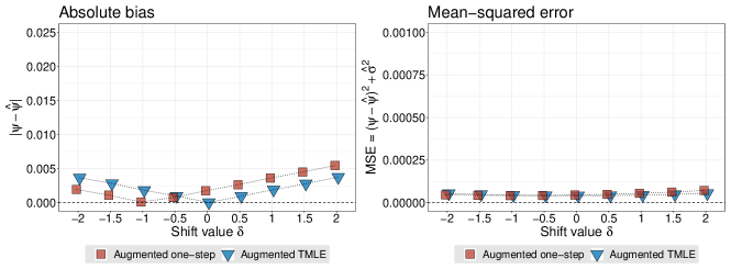
Figure 2: Results of numerical simulations comparing our two proposed estimators of $\psi_{0,\delta}$ for a grid of $\delta$, across 1000 Monte Carlo simulations at $n=1400$.

Inspection of the bias and MSE indicates that both of our proposed estimators display adequate performance, with small finite-sample bias and mean-squared error. In terms of bias and MSE, the performance of the two estimators is nearly indistinguishable. From these numerical investigations, we concluded that our augmented estimators are both well-suited to estimating $\psi_{0,\delta}$ in the context of a re-analysis of data from the HVTN 505 trial.

5 Application to the HVTN 505 Trial

The HVTN 505 trial was a randomized control trial that enrolled $2504$ HIV-negative participants and randomized participants 1-to-1 to receive an active vaccine or placebo. The one-year incidence of HIV-1 infection was about 1.8% per person-year in the vaccine arm and 1.4% per person-year in the placebo arm, during primary follow-up for HIV-1 acquisition (between week 28 and month 24; the same period as was used for assessment of immune correlates). Blood was drawn post-vaccination and immune responses measured via intracellular cytokine staining of preserved HIV-1-stimulated peripheral blood mononuclear cells for all HIV-1 cases diagnosed between week 28 and month 24 and a random sample of uninfected controls (Janes et al., 2017). The two-phase sampling of vaccine recipient controls without-replacement sampled five controls per case within each of eight baseline covariate strata defined by categories of body mass index and race/ethnicity (White, Hispanic, Black). Janes et al. (2017) provide the first immune correlates analysis of the HVTN 505 data based on the constructed two-phase sample, focusing on two cellular immune responses: the Envelope CD4+ and CD8+ polyfunctionality scores. Subsequently, Fong et al. (2018) analyzed an expanded set of immune markers, including six primary humoral immune response variables beyond the two first studied by Janes et al. (2017). Both sets of analyses found the CD4+ and CD8+ polyfunctionality scores to be informative of HIV-1 infection status by month 24 of the study (end of follow-up).

We examined how a range of posited shifts in standardized polyfunctionality scores of the CD4+ and CD8+ immune markers would impact the mean counterfactual risk of HIV-1 infection in vaccine recipients. We considered standardized polyfunctionality scores, so that our pre-specified grid of shifts $\delta\in\{-2.0,-1.5,-1.0,-0.5,\allowbreak 0.0,0.5,1.0,1.5,2.0\}$ can be interpreted as shifts on the scale of standard deviation (sd). We present results based on our TML estimator; results for the one-step estimator were similar. In order to summarize the manner in which the mean counterfactual risk of HIV-1 infection varies with shifts in the polyfunctionality scores, we consider projection onto a linear working MSM, as discussed in section 3.4. Our augmented TML estimator $\psi_{n,\delta}^{\star}$ for the mean counterfactual risk of HIV-1 infection requires the construction of initial estimators of all nuisance functions.

We used flexible estimation strategies for each of the nuisance parameters. The conditional probability of inclusion in the second-phase sample was estimated using HAL, adjusting for age, sex, race/ethnicity, body mass index, and a behavioral risk score for HIV-1 infection. The density $q_{n,A}$ of the CD4+ or CD8+ polyfunctionality scores, conditional on the same set of covariates, was estimated using our proposed HAL-based density estimator (Hejazi et al., 2020). The outcome regression $\overline{Q}_{0,Y}$ was estimated using super learner (van der Laan et al., 2007), which was used to build an ensemble model as a weighted combination of prediction functions from a diverse collection of candidate algorithms. Further details, including choices of learning algorithms and weights assigned to each by the super learner ensemble, are given in section LABEL:supp:hvtn_sl_details of the Supplementary Materials. The pseudo-outcome regression, $G_{n}$, was fit via HAL.

We note that our choice of estimation strategy — specifically, the use of HAL regression for $g_{0,C}$ and HAL-based conditional density estimation for $q_{0,A}$ — ensures a sufficiently fast rate of convergence of these nuisance parameter estimates to their true values under only mild assumptions. Importantly, this allows for the second case described in lemma 1 to be fulfilled, ensuring consistency of the resultant TML estimates. This consistency of the estimates would hold even in the case that the HAL regression and super learner ensembles used for $G_{0}$ and $Q_{0,Y}$, respectively, proved inconsistent; however, as both of these nuisance parameters are also estimated via flexible modeling approaches, it would be expected that the conditions of theorem 1 are made to hold. Thus, we expect that our TML estimates of the counterfactual risk of HIV-1 infection across the grid in $\delta$ will be consistent and (quite possibly) nonparametric-efficient. Taking advantage of the robustness built into our estimation strategy lends an additional degree of reliability as to the results of our analysis of the HVTN 505 data. Finally, we recall that the estimate of $\beta_{0}$, the slope of the marginal structural model through the TML estimates of the counterfactual risk in $\delta$, is endowed with the same consistency and efficiency properties as the individual TML estimates.

Results of applying our estimation procedure separately to both the CD4+ and CD8+ polyfunctionality scores are presented in Figure 3.

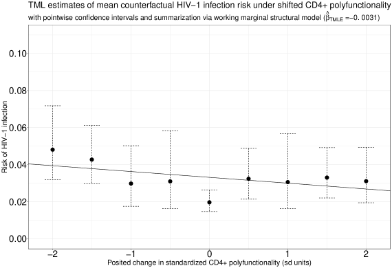
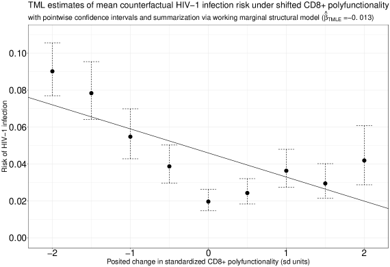
Figure 3: TML estimates of the counterfactual mean of HIV-1 infection under stochastic interventions on CD4+ (top) and CD8+ (bottom) standardized polyfunctionality scores. Inference for the estimates is based on pointwise Wald-type confidence intervals. The slope of a linear working MSM $\hat{\beta}_{\text{TMLE}}$ summarizes the effect of shifting the polyfunctionality scores on the mean counterfactual risk of HIV-1 infection.

Examination of the point estimates and confidence intervals of $\psi_{0,\delta}$ in Figure 3 reveals that downshifts in the CD4+ polyfunctionality score led to a small increase in estimated HIV-1 infection risk (Figure 3, top panel). For example, a shift of two standard units lower in the CD4+ polyfunctionality score was found to double the risk of HIV-1 infection. The estimated slope parameter of the working MSM $\hat{\beta}_{\text{TMLE}}$ pointed to an estimated decrease in risk of about -0.3% per standard unit of CD4+ polyfunctionality change.

The estimated result of shifts in the polyfunctionality score of the CD8+ immunogenic marker displayed a markedly much stronger relationship with the risk of HIV-1 infection (Figure 3, lower panel). While positive shifts of the standardized CD8+ polyfunctionality score beyond those observed in the trial do not appear to have a strong effect on HIV-1 infection risk, shifts that lower the CD8+ polyfunctionality score display a negative linear trend, indicating that decreases in CD8+ marker activity adversely affect the risk of HIV-1 infection. At the largest negative shift considered, the counterfactual HIV-1 infection risk is over four times that observed in the HVTN 505 trial.

Overall, the results of our analyses support the conclusions of Janes et al. (2017) and Fong et al. (2018), further indicating that modulation of the CD4+ and CD8+ polyfunctionality scores may reduce the risk of HIV-1 infection, with CD8+ polyfunctionality playing a particularly important role. Notably, our analysis differs from the previous efforts in two ways: our estimates (i) are based on a formal causal model, which provides an alternative estimand to summarize relationships between immunogenic response and risk of HIV-1 infection, and (ii) leverage machine learning to allow the use of flexible modeling strategies while simultaneously delivering robust inference.

6 Discussion

Our analysis of the HVTN 505 trial could be improved in several respects. First, there was participant dropout observed in the trial, which our analysis ignored. A more robust analysis could leverage available covariate information to account for potentially informative missingness. Beyond this issue, there are several other directions for potentially interesting extensions. It would be of interest to extend our estimation strategy to other effects based on stochastic interventions, including the population intervention (in)direct effects (Díaz and Hejazi, 2020) defined in mediation analysis and the incremental propensity score interventions of Kennedy (2019). Extending our estimation strategy to such settings and its application in analyzing other vaccine efficacy trials will be the subject of future research.

References

- Benkeser and van der Laan (2016) Benkeser, D. and van der Laan, M. J. (2016). The highly adaptive lasso estimator. In Data Science and Advanced Analytics (DSAA), 2016 IEEE International Conference on, pages 689–696. IEEE.
- Bibaut and van der Laan (2019) Bibaut, A. F. and van der Laan, M. J. (2019). Fast rates for empirical risk minimization with cadlag losses with bounded sectional variation norm. arXiv preprint arXiv:1907.09244 .
- Bickel et al. (1993) Bickel, P. J., Klaassen, C. A., Ritov, Y., and Wellner, J. A. (1993). Efficient and adaptive estimation for semiparametric models. Johns Hopkins University Press Baltimore.
- Breslow and Cain (1988) Breslow, N. and Cain, K. (1988). Logistic regression for two-stage case-control data. Biometrika 75, 11–20.
- Breslow et al. (2003) Breslow, N., McNeney, B., Wellner, J. A., et al. (2003). Large sample theory for semiparametric regression models with two-phase, outcome dependent sampling. The Annals of Statistics 31, 1110–1139.
- Breslow and Holubkov (1997) Breslow, N. E. and Holubkov, R. (1997). Maximum likelihood estimation of logistic regression parameters under two-phase, outcome-dependent sampling. Journal of the Royal Statistical Society: Series B (Statistical Methodology) 59, 447–461.
- Breslow et al. (2009a) Breslow, N. E., Lumley, T., Ballantyne, C. M., Chambless, L. E., and Kulich, M. (2009a). Improved horvitz–thompson estimation of model parameters from two-phase stratified samples: applications in epidemiology. Statistics in biosciences 1, 32–49.
- Breslow et al. (2009b) Breslow, N. E., Lumley, T., Ballantyne, C. M., Chambless, L. E., and Kulich, M. (2009b). Using the whole cohort in the analysis of case-cohort data. American Journal of Epidemiology 169, 1398–1405.
- Brown (2014) Brown, D. M. (2014). Applications of Causal Inference to Problems of Occupational Epidemiology. PhD thesis, UC Berkeley.
- Chatterjee and Chen (2007) Chatterjee, N. and Chen, Y.-H. (2007). A semiparametric pseudo-score method for analysis of two-phase studies with continuous phase-i covariates. Lifetime data analysis 13, 607–622.
- Chatterjee et al. (2003) Chatterjee, N., Chen, Y.-H., and Breslow, N. E. (2003). A pseudoscore estimator for regression problems with two-phase sampling. Journal of the American Statistical Association 98, 158–168.
- Chen and Chen (2000) Chen, Y.-H. and Chen, H. (2000). A unified approach to regression analysis under double-sampling designs. Journal of the Royal Statistical Society: Series B (Statistical Methodology) 62, 449–460.
- Chernozhukov et al. (2016) Chernozhukov, V., Chetverikov, D., Demirer, M., Duflo, E., Hansen, C., and Newey, W. K. (2016). Double machine learning for treatment and causal parameters. Technical report, cemmap working paper.
- Coyle et al. (2019) Coyle, J. R., Hejazi, N. S., and van der Laan, M. J. (2019). hal9001: The scalable highly adaptive lasso. R package version 0.2.5.
- Dai et al. (2009) Dai, J. Y., LeBlanc, M., and Kooperberg, C. (2009). Semiparametric estimation exploiting covariate independence in two-phase randomized trials. Biometrics 65, 178–187.
- Díaz and Hejazi (2020) Díaz, I. and Hejazi, N. S. (2020). Causal mediation analysis for stochastic interventions. Journal of the Royal Statistical Society: Series B (Statistical Methodology) .