The D model for deaths by COVID-19

Abstract

We present a simple analytical model to describe the fast increase of deaths produced by the corona virus (COVID-19) infections. The ’D’ (deaths) model comes from a simplified version of the SIR (susceptible-infected-recovered) model known as SI model. It assumes that there is no recovery. In that case the dynamical equations can be solved analytically and the result is extended to describe the D-function that depends on three parameters that we can fit to the data. Results for the data from Spain, Italy and China are presented. The model is validated by comparing with the data of deaths in China, which are well described. This allows to make predictions for the development of the disease in Spain and Italy.

1 Introduction

The SIR (susceptible-infected-recovered) model, developed by Ross, Hamer, and others [1], is widely used among the many epidemiological models as a first approach to virus spreading, with applications to many other sociological situations [2]. It consists of a system of three coupled non-linear ordinary differential equations [3] involving three time-dependent functions:

• Infected individuals, $I(t)$.

• Susceptible individuals, $S(t)$.

• Recovered individuals, $R(t)$.

The resulting dynamical system is the following

$$\frac{dS}{dt} = -\lambda SI$$ (1)

$$\frac{dI}{dt} = \lambda SI-\beta I$$ (2)

$$\frac{dR}{dt} = \beta I$$ (3)

$$S(t)+I(t)+R(t) = N$$ (4)

where $\lambda>0$ is the corona virus transmission rate, $\beta>0$ is the recovery rate, and $N$ is the total population size. The system is reduced to two coupled differential equations, which does not possess an explicit formula solution, but can be solved numerically. The SIR model is usually parametrized using actual infection data and the solution of the $I(t)$ function can be compared with actual infection data, to predict the evolution of the disease.

In this paper we make drastic assumptions in order to obtain an analytical formula to describe the evolution of deaths by corona virus. This can be useful as a fast method to foresee the global behavior as a first approach before applying more sophisticated methods. We shall see that the resulting ’D’ (deaths) model, that derivates from the SI model (no recovery), and is extended to deaths, describes well enough the data of the current corona virus pandemic in the countries China, Spain and Italy, where the pandemic is stronger.

2 The D model

The first basic assumption of the model is that there is no recovery from corona virus, at least during the pandemic time interval. This drastic assumption could be reasonable if the spreading time of the pandemic is much faster than the recovery time, or $\beta\ll\lambda$.

Under this simple assumption $R(t)=0$, and the SIR equations reduce to the single equation of the well known SI model

$$\frac{dI}{dt}=\lambda(N-I(t))I(t).\\$$ (5)

Therefore the infection rate is proportional to the infected, $I$ and to the non-infected $N-I$ or susceptible individuals.

This equation is easily solved in the following way. Dividing by $(N-I)I$ and multiplying by $dt$,

$$\frac{dI}{(N-I)I}=\lambda dt$$ (6)

or

$$\left(\frac{1}{N-I}+\frac{1}{I}\right)dI=\lambda Ndt$$ (7)

Integrating over $t=0$ and $t$ we obtain

$$\ln\frac{I}{N-I}-\ln\frac{I_{0}}{N-I_{0}}=\lambda N(t-t_{0})$$ (8)

Where $I_{0}=I(t_{0})$. Taking the exponential on both sides

$$\frac{I}{N-I}=\frac{I_{0}}{N-I_{0}}{\rm e}^{\lambda N(t-t_{0})}$$ (9)

Finally, solving this algebraic equation we obtain the solution $I(t)$

$$I(t)=\frac{NI_{0}{\rm e}^{\lambda N(t-t_{0})}}{N-I_{0}+I_{0}{\rm e}^{\lambda N(t-t_{0})}}$$ (10)

We write this equation in the form

$$I(t)=\frac{I_{0}\,{\rm e}^{(t-t_{0})/b}}{1-C+C\,{\rm e}^{(t-t_{0})/b}}$$ (11)

Where we have defined the constants

$$b=\frac{1}{\lambda N},\kern 28.45274ptC=\frac{I_{0}}{N}$$ (12)

The parameter $b$ is the characteristic evolution time of the initial exponential increase of the pandemic. The constant $C$ is the initial infestation rate (with respect to the total population). Assuming that initially $C\ll 1$, this constant can be neglected in the denominator, obtaining

$$I(t)=\frac{I_{0}\,{\rm e}^{(t-t_{0})/b}}{1+C\,{\rm e}^{(t-t_{0})/b}}$$ (13)

Now to predict the number of deaths in the D model we assume that the number of deaths at some time $t$ is proportional to the infestation at some former time $\tau$, that is,

$$D(t)=mI(t-\tau)$$ (14)

Where $m$ is the mortality or death rate, and $\tau$ is the mortality time.

With this assumption we can finally write the D model equation as

$$D(t)=\frac{a{\rm e}^{(t-t_{0})/b}}{1+c\,{\rm e}^{(t-t_{0})/b}}$$ (15)

where $a=mI_{0}\,{\rm e}^{-\tau/b}$, and $c=C\,{\rm e}^{-\tau/b}$. This is the final equation for the model. This simple function has three parameters, $a,b,c$, which we fit to the data. Note that the rest of the parameters, $m$, $\tau$, $I_{0}$ and $N$ are not needed in our model because they are included inside the fitted parameters $a,b,c$.

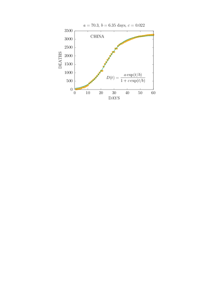
Figure 1: Fit of the D-model to the deaths by corona virus in China. Data are from [4].

3 Results

In this section we fit the three parameters, $a,b,c$ of our model, Eq. (15), to real data for three countries, China, Spain and Italy. The data are taken from ref. [4]

In Fig, 1 we show our fit of the D-model to the death data of China. In this country the evolution has been apparently controlled and the D function has already arrived to the plateau zone, with few increments over time, or fluctuations that are beyond the model assumptions. We see that the pandemic lasted for about two months to reach the top end of the curve. Fig. 1 shows that the model describes well the COVID-19 evolution of deaths, despite our crude assumptions. This validation allows us to trust its applicability in other cases where the pandemic is still in its initial phase, to make predictions.

Figure 2: Fit of the D-model to the deaths by corona virus in Spain. Data are from [4].

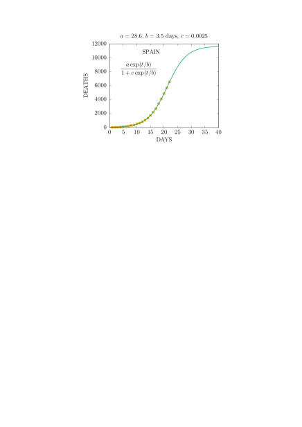
Figure 3: Prediction of the D-model to the COVID-19 pandemic in Spain. Data are from [4].

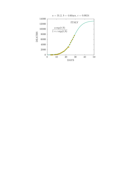
Figure 4: Prediction of the D-model to the COVID-19 pandemic in Italy. Data are from [4].

In Fig, 2 we show our fit of the D-model to the death data of Spain. The data start on March, 8 2020 (day 1). In this country the evolution has been strong and up to day 22 (March 29 2020) they have exceeded the deaths in china, reaching almost 7000 deaths. In Fig. 2 we see that the D-model describes quite well this evolution region up to day 22 of the pandemic.

In fig.3 we show our prediction for the next weeks in Spain, using the fit to the first 22 days. According to the figure we reached the mid point of the curve on day 21. It is expected that Spain will reach the top plateau of the curve in 18 days, that is in mid April.

Finally in Fig. 4 we show our fit and prediction to the Italy data. The parameters are similar to the case of Spain with about 20 days to the top of the curve.

4 Final remarks

To conclude we have seen that the D-model for COVID-19 pandemic, derived form the SI model, describes well the current data of China, Spain and Italy with only three parameters.

The assumption made here, that the recovered individual do not influence the increase of the infected, could further indicate that the total population $N$ is not a constant as assumed in the SIR model, but it increases over time as more people are exposed, for example, in villages that until now had been isolated from the sources of infection in big cities.

The D model is simple enough to provide fast estimations of pandemic evolution in other countries, and could be useful for the control of the disease.

5 Acknowledgements

The author thanks useful comments from Nico Orce and from the WhatsApp group Covid-19.

This work is supported by Spanish Ministerio de Economia y Competitividad and European FEDER funds (grant FIS2017-85053-C2-1-P) and Junta de Andalucia (grant FQM-225).

References

- [1] R. M. Anderson, Discussion: the Kermack-McKendrick epidemic threshold theorem. Bulletin of mathematical biology, 53(1): 1–32, 1991.
- [2] H.S. Rodrigues, Application of SIR epidemiological model: new trends, arXiv:1611.02565 (2016)
- [3] H. Weiss, The SIR model and the Foundations of Public Health, MATerials MATematics Volum 2013, treball no. 3, 17 pp.
- [4] https://www.worldometers.info/coronavirus/