A generalized permutation entropy for random processes

Abstract

Permutation entropy measures the complexity of deterministic time series via a data symbolic quantization consisting of rank vectors called ordinal patterns or just permutations. The reasons for the increasing popularity of this entropy in time series analysis include that (i) it converges to the Kolmogorov-Sinai entropy of the underlying dynamics in the limit of ever longer permutations, and (ii) its computation dispenses with generating and ad hoc partitions. However, permutation entropy diverges when the number of allowed permutations grows super-exponentially with their length, as is usually the case when time series are output by random processes. In this Letter we propose a generalized permutation entropy that is finite for random processes, including discrete-time dynamical systems with observational or dynamical noise.

Keywords Nonlinear time series analysis  $\cdot$ Permutation entropy  $\cdot$ Random processes  $\cdot$ Noisy deterministic signals

1 Introduction

In general, time series result from observing real-valued random processes or dynamical flows at discrete times. A further step may be the discretization of the data, a procedure called symbolic representation. Such representations simplify the mathematical tools needed for the data analysis and, what is more interesting for practitioners, may be sufficient for the application sought. In this regard, ordinal patterns and permutation entropy have become increasingly popular in nonlinear time series analysis since their introduction by Bandt and Pompe in 2002 [1]. The reasons are multiple. Perhaps most importantly from a theoretical point of view, ordinal patterns, which are formally permutations, preserve the temporal structure of a time series and, therefore, its dynamical complexity. In fact, in one-dimensional dynamics the permutation entropy per symbol converges to the Kolmogorov-Sinai (KS) as the pattern length grows [2, 3, 4], which makes it a proxy of dynamical entropy. From a practical point of view, the computation of permutation entropy dispenses with ad hoc partitions, not to mention the search for generating ones [5]. But even with real-world series, which are usually rather noisy, tools such as permutation entropies of finite order and the decay rate of missing ordinal patterns have proved very handy [6, 7, 8]. Further advantages of the ordinal approach in the analysis of time series include speedy calculation, robustness to noise, the possibility of multiscale analysis through a varying pattern length, as well as high discriminatory power in the classification of data, especially in combination with other complexity indicators [9, 10, 11]. As a result, this methodology is being successfully applied in plenty of fields, e.g., chaotic dynamics, earth science, computational neuroscience, biomedicine, econophysics and more; see [12, 13, 14] for recent surveys.

More generally, the permutation entropy of a real-valued time series, whether deterministic or random, is just the Shannon entropy of its ordinal representation, i.e., the symbolic time series that results from replacing data strings of a fixed length $L\geq 2$ by the corresponding ordinal patterns of length $L$. There is a twist, though. Shannon’s entropy was incepted in the setting of finite-state random processes (information sources with finite alphabets), so that the number of states (words) grows exponentially with the length of the output (message). But in the ordinal representation of time series, each word of length $L$ is replaced by a permutation of $\{0,1,...,L-1\}$; if all permutations are allowed, as happens in general with real-valued random processes (including noisy chaotic signals), then the number of words grows super-exponentially with $L$ because $L!\simeq e^{L\ln L}$. Similarly, the number of microstates grows super-exponentially with the number of particles in some models of statistical mechanics, the realm of the Boltzmann-Gibbs entropy [15]. For this super-exponential class of processes and many-particle systems, the Boltzmann-Gibbs-Shannon (BGS) entropy is not extensive, meaning that it does not scale linearly over uniform probability distributions or, in thermodynamical terms, at equilibrium. Consequently, the BGS entropy per symbol or particle is unbounded and, in general, diverges. This is the case, in particular, with the permutation entropy for random processes.

In this Letter we propose a generalization of permutation entropy that is finite for random processes. To this end, we resort to a new entropy belonging to the class of group entropies, which is extensive and has several interesting statistical properties [16], as well as a normalized range. But before reaching to that point, we need to delve into permutation complexity, which stands for the complexity of discrete-time, continuous-state deterministic or random processes and their realizations in ordinal representations [17].

2 Permutation complexity

Given a time series $(x_{t})_{t\geq 0}=x_{0},x_{1},\ldots,x_{t},...$, with $t$ being discrete time and $x_{t}\in\mathbb{R}$, let $L\geq 2$ and denote by $\mathbf{r}_{t}$ the rank vector of the string (word, block, …) $x_{t}^{L}:=x_{t},x_{t+1},...,x_{t+L-1}$. That is,

$$\mathbf{r}_{t}=(\rho_{0},\rho_{1},\ldots,\rho_{L-1}),$$ (1)

where $\rho_{0},\rho_{1},\ldots,\rho_{L-1}$ is the permutation of $0,1,\ldots,L-1$ such that

$$x_{t+\rho_{0}}<x_{t+\rho_{1}}<\ldots<x_{t+\rho_{L-1}}$$ (2)

(other rules can be found in the literature). The rank vectors $\mathbf{r}_{t}$ are called ordinal patterns or permutations of length $L$, as well as ordinal $L$-patterns for short; the string $x_{t}^{L}$ is said to be of type $\mathbf{r}_{t}$. In case of two or more ties in $x_{t}^{L}$, one can adopt some convention, e.g., the earlier entry is smaller. We suppose tacitly that such occurrences are rare. As a result, the alphabet (set of symbols) of $(\mathbf{r}_{t})_{t\geq 0}$, the ordinal representation of the original time series $(x_{t})_{t\geq 0}$, is the group of the $L!$ permutations of $0,1,\ldots,L-1$, which will be denoted by $\mathcal{S}_{L}$.

Consider a stationary, discrete-time deterministic or random process $\mathbf{X}=(X_{t})_{t\geq 0}$ taking values on a closed interval $I\subset\mathbb{R}$. By a deterministic process we mean that every output $(x_{t})_{t\geq 0}$ of $\mathbf{X}$ is the orbit of $x_{0}$ generated by the same mapping $F:I\rightarrow I$, i.e., $x_{t+1}=F(x_{t})=F^{t}(x_{0})$ for $t\geq 0$. Therefore, random processes include deterministic ones with observational or dynamical noise, which are instances of random dynamical systems. Let $p(\mathbf{r})$ be the probability that a string $x_{t}^{L}$ output by $\mathbf{X}$ is of type $\mathbf{r}$ and $p=\{p(\mathbf{r}):\mathbf{r}\in\mathcal{S}_{L}\}$ the corresponding probability distribution. If $p(\mathbf{r})>0$, then $\mathbf{r}$ is an allowed pattern for $\mathbf{X}$; otherwise $\mathbf{r}$ is a forbidden pattern. The Shannon entropy (or the BGS entropy for that matter) of $p$ is called the (metric) permutation entropy of order $L$:

$$H^{\ast}(X_{0}^{L})=-\sum_{\mathbf{r}\in\mathcal{S}_{L}}p(\mathbf{r})\ln p(\mathbf{r}),$$ (3)

where $X_{0}^{L}:=X_{0},X_{1},\ldots,X_{L-1}$ and $0\cdot\ln 0:=0$ by continuity. In the event that $\mathbf{X}$ is a deterministic process, $p(\mathbf{r})=\mu(\{x_{t}\in I:x_{t}^{L}$ is of type $\mathbf{r}\})$, where $\mu$ is the physical measure of $\mathbf{X}$, which is an $F$-invariant measure that coincides with the empirical probability distribution [18]. If, otherwise, $\mathbf{X}$ is a random process, then the probabilities $p(\mathbf{r})$ can only exceptionally be derived from the probability distribution of $X_{t}^{L}$ [19] so, in general, they have to be estimated, e.g., by the relative frequencies of each $\mathbf{r}\in\mathcal{S}_{L}$ in a finite time series $x_{0},x_{1},....,x_{T}$,

$$\nu(\mathbf{r})=\frac{\#\{x_{t}^{L}\text{ of type }\mathbf{r}\in\mathcal{S}_{L}:0\leq t\leq T-L+1\}}{T-L+2},$$ (4)

where $\#$ stands for “number of” and $T\gg L!$ (maximum likelihood estimator). Then, $p(\mathbf{r})=\lim_{T\rightarrow\infty}\nu(\mathbf{r})$, where this limit exists with probability 1 when the underlying random process fulfills the following weak condition [1].

Stationarity Condition. For $k\leq L-1$, the probability for $x_{t}<x_{t+k}$ should not depend on $t$.

Random processes that meet this condition include, in addition to stationary ones, non-stationary processes with stationary increments such as fractional Brownian motion and fractional Gaussian noise. From now on we assume the Stationarity Condition so that estimations of $p(\mathbf{r})$ converge as the amount of data increases.

The topological permutation entropy of order $L$ is the tight upper bound of $H^{\ast}(X_{0}^{L})$. It is formally obtained by assuming that all allowed $L$-patterns are equiprobable:

$$H_{0}^{\ast}(X_{0}^{L})=\ln\mathcal{N}_{L}(\mathbf{X}),$$ (5)

where $\mathcal{N}_{L}(\mathbf{X})$ is the number of allowed patterns of length $L$ for $\mathbf{X}$. In turn, the metric and topological permutation entropies of a process $\mathbf{X}$ are obtained by taking the corresponding entropies of order $L$ per symbol and letting $L\rightarrow\infty$,

$$h^{\ast}(\mathbf{X})=\lim_{L\rightarrow\infty}\frac{1}{L}H^{\ast}(X_{0}^{L}),\;h_{0}^{\ast}(\mathbf{X})=\lim_{L\rightarrow\infty}\frac{1}{L}H_{0}^{\ast}(X_{0}^{L}),$$ (6)

provided that the limits exist. More conveniently, one can use “$\lim\sup$” (limit superior) instead of “$\lim$” to ensure that these and the forthcoming limits converge or diverge to $+\infty$. We elaborate next on the fact that permutation entropy is finite for deterministic processes while diverging for random processes in general.

A mapping $F:I\rightarrow I$ is said to be piecewise monotone if there is a finite partition of $I$ such that $F$ is continuous and monotone on each subinterval of the partition. Let $h(F)$ be the KS entropy of $F$, and $h_{0}(F)$ its topological entropy [20]. The following theorem, proved in [2], holds.

Theorem 1. If $F$ is piecewise monotone, then (i) $h^{\ast}(F)=h(F)$ and (ii) $h_{0}^{\ast}(F)=h_{0}(F)$.

All one-dimensional mappings encountered in practice are piecewise monotone, so we may assume this property for the mappings underlying deterministic processes. Therefore, $h^{\ast}(\mathbf{X})\leq h_{0}^{\ast}(\mathbf{X})<\infty$ for deterministic processes since $h_{0}(F)<\infty$ for piecewise monotone mappings [21]. Incidentally, Theorem 1(ii) implies $\mathcal{N}_{L}(\mathbf{X})\sim e^{h_{0}(F)L}$ ($\sim$ stands for “asymptotically”), meaning that such processes have only exponentially many allowed $L$-patterns for ever larger $L$’s, despite the fact that there are $L!\sim e^{L\ln L}=L^{L}$ (Stirling’s formula) possible ordinal $L$-patterns. The upshot is that the number of forbidden patterns for deterministic processes grows super-exponentially with $L$ [22]. Also higher dimensional dynamics along with their lower dimensional projections may have forbidden patterns [23]. However, if the dynamics takes place on an attractor, so that the orbits are dense, then the observational or dynamical noise will ‘destroy’ all forbidden patterns in the long run, no matter how small the noise. Theorem 1 was generalized in [24].

On the other hand, random processes may have forbidden patterns too. For the sake of our analysis, though, we will consider the general or ‘worse’ scenario in which all ordinal patterns of any length are allowed. A necessary and sufficient condition for this is that, for $k\leq L-1$, the probability for $x_{t}<x_{t+k}$ is neither 0 nor 1 (so that the same holds for $x_{t}>x_{t+k}$), which amounts to a mild addendum to the Stationarity Condition. With this proviso, we assume hereafter $\mathcal{N}_{L}(\mathbf{X})=L!$ for all random processes $\mathbf{X}$. Then,

$$h_{0}^{\ast}(\mathbf{X})=\lim_{L\rightarrow\infty}\frac{1}{L}\ln L!=\lim_{L\rightarrow\infty}\ln L=\infty$$ (7)

by Stirling’s formula. We conclude from (7) that permutation entropy, unlike Shannon’s entropy, cannot be applied to random processes in general. In particular, $H^{\ast}(X_{0}^{L})$ does not scale linearly when $L\rightarrow\infty$ over flat probability distributions.

Numerical evidence is shown in Fig. 1. Here we have numerically generated 10 realizations of size $T\gtrsim 50L!$ (see (4)) of the following processes: (i) white noise (WN) in the form of an independent and uniformly distributed process on $[0,1]$; (ii) fractional Gaussian noise (fGn) with Hurst exponent $H=0.5$ (Gaussian white noise); (iii) noise with an $f^{-1}$ power spectrum (PS); (iv) fractional Brownian motion (fBm) with $H=0.25$ (anti-persistent process), $0.5$ (classical Brownian motion), and $0.75$ (persistent process). Computations were done with MatLab [25]. The average of $H^{\ast}(X_{0}^{L})/L$ over the 10 realizations of each process, denoted $\langle H^{\ast}(X_{0}^{L})/L\rangle$, is then plotted against $L$, $3\leq L\leq 8$. We see in all cases that $\langle H^{\ast}(X_{0}^{L})/L\rangle$ follows a seemingly divergent trajectory as $L$ grows.

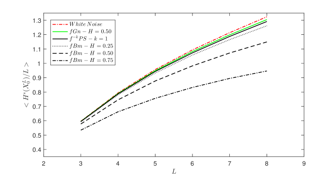
Figure 1: The average of $H^{\ast}(X_{0}^{L})/L$ over 10 realizations, $\langle H^{\ast}(X_{0}^{L})/L\rangle$, is plotted vs $L$ for $1\leq L\leq 8$ and the random processes listed in the inset. See the text for detail.

3 Group entropies

The theory of group entropies [26, 27, 28, 29] is an axiomatic approach which allows us to construct information measures with mathematical properties that make them suitable to describe specific universality classes of complex systems (see [30] for a review). We recap here some basic definitions.

Let $\mathcal{P}_{W}$ be the set of all discrete probability distributions with $W$ entries, i.e., $\mathcal{P}_{W}=\{p=(p_{i})_{i=1,\cdots,W}:0\leq p_{i}\leq 1,\,\sum_{i=1}^{W}p_{i}=1\}$. Let $S$ be a non-negative function on $\mathcal{P}:=\cup_{W=1}^{\infty}\mathcal{P}_{W}$, so that $S$ is defined on any probability distribution $p$ and $S(p)\geq 0$. The Shannon-Khinchin (SK) axioms are a set of requirements first considered in [31], [32], [33] to uniquely characterize the BGS entropy. The first three SK axioms amount to the following properties:
(SK1) $S(p)$ is continuous with respect to all variables $p_{1},\ldots,p_{W}$.
(SK2) $S(p)$ takes its maximum value over the uniform distribution.
(SK3) $S(p)$ is expansible: adding an event of zero probability does not affect the value of $S(p)$.

These axioms represent a minimal set of ‘non-negotiable’ requirements that such functions $S(p)$ should satisfy necessarily to be meaningful, both from a physical and information-theoretical point of view. Non-negative functions on $\mathcal{P}$ that verify axioms (SK1)-(SK3) are called generalized entropies and their structure is only known under additional conditions [34, 35, 16]. Thus, the fourth SK axiom, requiring specifically additivity on conditional distributions, leads to the BGS entropy [33],

$$S_{BGS}(p)=-k\sum_{i=1}^{W}p_{i}\ln p_{i},$$ (8)

where $k$ is a positive constant that we equate to $1$ for definiteness (as in (3)). Instead, the more general axiom of composability (see below) leads to the new concept of group entropy. As we will discuss shortly, this entropy, which includes $S_{BGS}(p)$, is better suited to deal with the diversity of themodynamical and complex systems. Another independent approach, based on the concept of pseudo-additive entropy, was formulated in [36].

An entropy $S(p)$ is said to be composable if there exists a smooth function $\Phi(x,y)$ such that

$$S(p_{A}\times p_{B})=\Phi(S(p_{A}),S(p_{B}))$$ (9)

for any probability distributions $p_{A}$ and $p_{B}$, where $p_{A}\times p_{B}$ is the product probability distribution of both. Equivalently, (9) can be written as $S(A\cup B)=\Phi(S(A),S(B))$, where $A$ and $B$ are two statistically independent subsystems of a complex system, defined over any arbitrary probability distributions $p_{A}$ and $p_{B}$, respectively, and $A\cup B$ is the system composed of $A$ and $B$. All quantities are assumed to be dimensionless.

In addition to Equation (9), we shall also require the following properties for the composition law $\Phi$:
(C1) Symmetry: $\Phi(x,y)=\Phi(y,x)$.
(C2) Associativity: $\Phi(x,\Phi(y,z))=\Phi(\Phi(x,y),z)$.
(C3) Null-composability: $\Phi(x,0)=x$.

Observe that, indeed, requirements (C1)-(C3) are crucial: they impose the independence of the composition process with respect to the order of $A$ and $B$, the possibility of composing three independent subsystems in an arbitrary way, and the requirement that, when composing a system with another one having zero entropy, the total entropy remains unchanged. In our opinion, these properties are also fundamental: no thermodynamical or information-theoretical applications would be easily conceivable without these properties. For $\Phi(x,y)=x+y$ we obtain from (9) the additivity of the BGS entropy (8) with respect to the composition of two statistically independent subsystems.

From an algebraic point of view, the requirements (C1)-(C3) define a formal group law for a function (infinite series) of the form $\Phi(x,y)=x+y\,+$ $O(2)$, where $O(n)$ stands for terms of degree $\geq n$.

Definition 1. A group entropy is a function $S:\mathcal{P}\rightarrow[0,\infty)$ which satisfies the Shannon-Khinchin axioms (SK1)-(SK3) and the composability axiom (9).

A well-known group entropy, introduced by Tsallis in [37], is

$$S_{\alpha}(p)=\frac{1}{1-\alpha}\left(\sum\limits_{i=1}^{W}p_{i}^{\alpha}-1\right)$$ (10)

for $\alpha>0$, $\alpha\neq 1$, and $S_{1}(p):=$ $\lim_{\alpha\rightarrow 1}S_{\alpha}(p)=S_{BGS}(p)$, whose composition law is

$$\Phi(x,y)=x+y+(1-\alpha)xy,$$ (11)

so that $S_{\alpha}(p_{A}\times p_{B})=S_{\alpha}(p_{A})+S_{\alpha}(p_{B})+(1-\alpha)S_{\alpha}(p_{A})S_{\alpha}(p_{B})$. Except for the Tsallis entropy, group entropies have in general non-trace forms [38], that is, they cannot be written as $\sum_{i=1}^{W}g(p_{i})$, where $g:[0,1]\rightarrow[0,\infty)$ is a mapping with suitable properties, usually continuity, $\cap$-convexity and $g(0)=0$ [34].

As has been shown in [16, 30], one can classify complex systems according to their state space growth rate $\mathcal{W}(N)$, which counts the number of microstates allowed as a function of the number $N$ of particles or constituents of a given system, for large $N$. Generally speaking, we distinguish sub-exponential, exponential and super-exponential regimes with regard to the state space growth rate (which can be further discriminated if necessary). All systems that are characterized by the same asymptotic behavior of $\mathcal{W}$ define a universality class. According to Theorem 1 of [16], under mild hypotheses one can explicitly construct a suitable group entropy associated with a given universality class of systems, which would play the role of information or complexity measure for the class considered. This specific entropy (actually, a one-parametric family of entropies) is called a $Z$-entropy [27] and is denoted by $Z_{G,\alpha}(p)$, where $G$ refers to the underlying group-theoretical structure associated with it, $\alpha>0$, $p\in\mathcal{P}_{W}$ and $W=\left\lfloor\mathcal{W}(N)\right\rfloor$.

Moreover, there is a unique $Z_{G,\alpha}(p)$ entropy which is extensive for the systems of a given class, that is, if $Z_{G,\alpha}(N):=Z_{G,\alpha}(\frac{1}{W},...,\frac{1}{W})$ is the $Z$-entropy over the uniform distribution (the most ‘disordered’ situation), then

$$\lim_{N\rightarrow\infty}\frac{Z_{G,\alpha}(N)}{N}=~{}\text{const.}$$ (12)

In other words, $Z_{G,\alpha}(N)$, the topological version of $Z_{G,\alpha}(p)$, scales linearly with $N$, at least for $N$ sufficiently large. According to (SK2), $Z_{G,\alpha}(p)\leq Z_{G,\alpha}(N)$ for all $p\in\mathcal{P}_{W}$.

Prototypical examples of $Z$-entropies are (i) the Tsallis entropy $S_{\alpha}(p)$, Equation (10), for the sub-exponential class, and (ii) the Rényi entropy [39]

$$R_{\alpha}(p)=\frac{1}{1-\alpha}\ln\left(\sum\limits_{i=1}^{W}p_{i}^{\alpha}\right)$$ (13)

for $\alpha>0$, $\alpha\neq 1$, and $R_{1}(p):=\lim_{\alpha\rightarrow 1}R_{\alpha}(p)=S_{BGS}(p)$, for the exponential class. Notice that $S_{\alpha}(p)=\frac{1}{1-\alpha}(\exp[(1-\alpha)R_{\alpha}(p)]-1)$. The $Z$-entropy for the super-exponential class is our next concern.

4 A generalized permutation entropy

In our context, where random processes are real-valued and blocks $x_{t}^{L}$ of size $L\geq 2$ are quantized by means of ordinal $L$-patterns $\mathbf{r}_{t}$, discrete probability distributions $p$ refer necessarily to the symbols $\mathbf{r}\in\mathcal{S}_{L}$ and hence the growth function is $\mathcal{W}(L)=L!\sim e^{L\ln L}$ under very weak conditions. This being the case, we propose the $Z$-entropy for the super-exponential class to measure permutation complexity. Such an entropy was introduced in [15] to describe the thermodynamic properties of the so-called pairing model, which represents an example of a Hamiltonian system possessing a super-exponential state space growth.

Specifically, we define the permutation $Z$-entropy of order $L$ of a process $\mathbf{X}=(X_{t})_{t\geq 0}$ as

$$Z_{\alpha}^{\ast}(X_{t}^{L})\equiv Z_{\alpha}(p)=\exp\left[\mathcal{L}\left(R_{\alpha}(p)\right)\right]-1$$ (14)

for $\alpha>0$, where $p\in\mathcal{P}_{L!}$ is the probability distribution of the ordinal $L$-patterns of $X_{t}^{L}$, $R_{\alpha}(p)$ is Rényi’s entropy (13) with $W=L!$, and $\mathcal{L}(x)$ denotes the principal branch of the real Lambert function. $\mathcal{L}(x)$ is a smooth function that is defined for $x\geq-1/e$ and satisfies the equation $\mathcal{L}(x)e^{\mathcal{L}(x)}=x$, hence $\mathcal{L}(0)=0$ and $\mathcal{L}(x)>0$ for $x>0$ [40]. The term $-1$ in (14) renders $Z_{\alpha}(p)=0$ in situations without uncertainty, i.e., when $p_{i_{0}}=1$ and $p_{i}=0$ for $i\neq i_{0}$.

From a conceptual point of view, $Z_{\alpha}(p)$ can be interpreted to be a suitable, extensive deformation of $R_{\alpha}(p)$, sharing with it many fundamental properties, except additivity. For example, $Z_{\alpha}^{\ast}(X_{t}^{L})$ inherits from $R_{\alpha}(p)$ its $\cap$-convexity for $0<\alpha\leq 1$ and decreasing monotonicity with respect to $\alpha$ [35], that is,

$$Z_{\alpha}^{\ast}(X_{t}^{L})\geq Z_{\beta}^{\ast}(X_{t}^{L})\;\;\text{for\ \ }\alpha<\beta,$$ (15)

because the function $e^{\mathcal{L}(x)}$ is strictly increasing and $\cap$-convex.

It is clear that $Z_{\alpha}(p)$ verifies the axioms (SK1)-(SK3) since $R_{\alpha}(p)$ is a group entropy and $e^{\mathcal{L}(x)}$ is strictly increasing. The composability of $Z_{\alpha}(p)$ for the growth function $\mathcal{W}(L)=e^{L\ln L}$ follows from Proposition 1 of [16] (with $\mathcal{W}^{-1}(\xi)=\exp[\mathcal{L}(\ln\xi)]$). Alternatively, one can directly check that if

$$\Phi(x,y) = e^{\mathcal{L[}(x+1)\ln(x+1)+(y+1)\ln(y+1)]}-1$$

$$= x+y-\tfrac{1}{2}x^{2}-2xy-\tfrac{1}{2}y^{2}+O(3),$$

then the composition law $Z_{\alpha}(p_{A}\times p_{B})=\Phi(Z(p_{A}),Z(p_{B}))$ holds for any probability distributions $p_{A}$ and $p_{B}$.

As with conventional permutation entropy, we define the topological permutation $Z$-entropy of order $L$ of a process $\mathbf{X}=(X_{t})_{t\geq 0}$ as the tight upper bound of $Z_{\alpha}^{\ast}(X_{t}^{L})$, which is obtained over the uniform distribution of ordinal $L$-patterns:

$$Z_{0}^{\ast}(X_{t}^{L})\equiv Z_{\alpha}(\tfrac{1}{L!},\ldots,\tfrac{1}{L!})=\exp\left[\mathcal{L}\left(\ln L!\right)\right]-1$$ (17)

since $R_{\alpha}(\tfrac{1}{L!},\ldots,\tfrac{1}{L!})=\ln L!$ for all $\alpha$. The notation $Z_{0}^{\ast}$ is justified because $\ln L!$ is formally obtained from (13) by setting $\alpha=0$. It follows (use $\mathcal{L}(x\ln x)=\ln x$ for $x\geq 1/e$)

$$\frac{Z_{0}^{\ast}(X_{0}^{L})}{L}=\frac{e^{\mathcal{L}\left(\ln L!\right)}-1}{L}\sim\frac{e^{\mathcal{L}\left(L\ln L\right)}-1}{L}=\frac{L-1}{L}\sim 1,$$ (18)

so that $Z_{\alpha}^{\ast}(p)$ is indeed extensive in the regime of factorial growth we are interested in.

Regarding the permutation $Z$-entropy of a random process $\mathbf{X}$,

$$z_{\alpha}^{\ast}(\mathbf{X})=\underset{L\rightarrow\infty}{\lim\sup}\frac{1}{L}Z_{\alpha}^{\ast}(X_{0}^{L}),$$ (19)

we highlight the following properties.

Theorem 2. (i) Normalized range: $0\leq z_{\alpha}^{\ast}(\mathbf{X})\leq 1$, where $z_{\alpha}^{\ast}(\mathbf{X})=0$ for deterministic processes and $z_{\alpha}^{\ast}(\mathbf{X})=1$ for white noise. (ii) Hierarchical order: $z_{\alpha}^{\ast}(\mathbf{X})\geq z_{\beta}^{\ast}(\mathbf{X})$ for $\alpha<\beta$.

To prove that $z_{\alpha}^{\ast}(\mathbf{X})=0$ for deterministic processes, we recall that, according to Theorem 1(ii), $\mathcal{N}_{L}(\mathbf{X})\sim e^{h_{0}(F)L}$, where $h_{0}(F)$ is the topological entropy of the mapping $F$ that generates $\mathbf{X}$. Therefore, if $p$ is the probability distribution of the $L$-patterns, then $R_{0}(p)=\ln\mathcal{N}_{L}(\mathbf{X})\sim h_{0}(F)L$ and

$$\frac{Z_{\alpha}^{\ast}(X_{0}^{L})}{L}\leq\frac{e^{\mathcal{L[}R_{0}(p)]}-1}{L}\sim\frac{e^{\mathcal{L}[h_{0}(F)L]}}{L}=\frac{h_{0}(F)}{\mathcal{L}[h_{0}(F)L]}\sim 0,$$ (20)

where we used $e^{\mathcal{L}(x)}=x/\mathcal{L}(x)$. Furthermore, that $z_{\alpha}^{\ast}(\mathbf{X})\leq 1$, with equality for white noise, follows from $Z_{\alpha}^{\ast}(X_{0}^{L})\leq Z_{0}^{\ast}(X_{0}^{L})$ and $\lim\sup_{L\rightarrow\infty}\frac{1}{L}Z_{0}^{\ast}(X_{0}^{L})=1$, see (18). Finally, the hierarchical order of $z_{\alpha}^{\ast}(\mathbf{X})$ is a direct consequence of (15).

As way of illustration, Fig. 2 shows $\langle Z_{\alpha}^{\ast}(X_{0}^{L})/L\rangle$, the average of the permutation entropy rate $Z_{\alpha}^{\ast}(X_{0}^{L})/L$ over the same 10 time series and for the same random processes as in Fig. 1, against $L$, $1\leq L\leq 8$, where $\alpha=0.5$ (a), $1$ (b) and $2$ (c). Contrarily to Fig. 1, we see in all panels of Fig. 2 that $\langle Z_{\alpha}^{\ast}(X_{0}^{L})/L\rangle$ follows a seemingly convergent trajectory as $L$ grows, upper bounded by the white noise. In agreement with (15), $\langle Z_{0.5}^{\ast}(X_{0}^{L})/L\rangle\geq\langle Z_{1}^{\ast}(X_{0}^{L})/L\rangle\geq Z_{2}^{\ast}(X_{0}^{L})/L\rangle$ for each process.

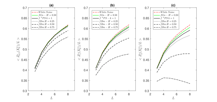
Figure 2: Same information as in Fig. 1 (but notice the different scale on the Y-axis) for $\langle Z_{0.5}^{\ast}(X_{0}^{L})/L\rangle$ (a), $\langle Z_{1}^{\ast}(X_{0}^{L})/L\rangle$ (b) and $\langle Z_{2}^{\ast}(X_{0}^{L})/L\rangle$ (c). See text for detail.

5 Conclusions

Summing up, the permutation $Z$-entropy $z_{\alpha}^{\ast}(\mathbf{X})$, Equations (19) and (14), measures the complexity of a real-valued random process $\mathbf{X}$ through permutations, where $\mathbf{X}$ is supposed to fulfill the Stationarity Condition and the mild assumption that all permutations are allowed for each length or, at least, a super-exponentially growing number of them. First and most importantly, $z_{\alpha}^{\ast}(\mathbf{X})$ is always finite, contrarily to what happens with $h^{\ast}(\mathbf{X})$, see Equation (7). Therefore, we may claim that $z_{\alpha}^{\ast}(\mathbf{X})$ generalizes the conventional permutation entropy to the realm of random processes. Further distinctive features are uniqueness [16] and the properties listed in Theorem 2. Applications include the analysis of data in general, and the characterization and classification of noisy signals in particular. In this regard, the parameter $\alpha$ is an asset because it enhances the discrimination capability of the ordinal approach. Since real-world series are finite, one has to use permutation $Z$-entropies of finite order $Z_{\alpha}^{\ast}(X_{0}^{L})$ in this case, where $L$ should be chosen so as to avoid undersampling of the ordinal $L$-patterns. Compared to $R_{\alpha}(p)$ and other entropies such as $S_{\alpha}(p)$, the expense of computing $Z_{\alpha}(p)$ is virtually the same. On these grounds, we propose $z_{\alpha}^{\ast}(\mathbf{X})$ as the right entropic measure to describe the complexity of real-valued random processes in ordinal representations.

Acknowledgments

J.M.A. was financially supported by the Spanish Ministry of Economy, Industry and Competitiveness (MINECO), grant MTM2016-74921-P (AEI/FEDER, EU). The research of P.T. has been partly supported by the research project PGC2018-094898-B-I00, MINECO, Spain, and by the ICMAT Severo Ochoa project SEV-2015-0554 (MINECO). P.T. is member of the Gruppo Nazionale di Fisica Matematica (INDAM), Italy.

References

- [1] C. Bandt and B. Pompe. Permutation entropy: A natural complexity measure for time series. Phys. Rev. Lett., 88:174102, Apr 2002.
- [2] C. Bandt, G. Keller, and B. Pompe. Entropy of interval maps via permutations. Nonlinearity, 15(5):1595–1602, aug 2002.
- [3] K. Keller. Permutations and the kolmogorov-sinai entropy. Discrete and Continuous Dynamical Systems - A, 32(1078):891, 2012.
- [4] J. M. Amigó. The equality of kolmogorov–sinai entropy and metric permutation entropy generalized. Physica D: Nonlinear Phenomena, 241(7):789 – 793, 2012.
- [5] Y. Hirata, K. Judd, and D. Kilminster. Estimating a generating partition from observed time series: Symbolic shadowing. Phys. Rev. E, 70:016215, Jul 2004.
- [6] V. A. Unakafova and K. Keller. Efficiently measuring complexity on the basis of real-world data. Entropy, 15(10):4392–4415, 2013.
- [7] A. M. Unakafov and K. Keller. Conditional entropy of ordinal patterns. Physica D: Nonlinear Phenomena, 269:94 – 102, 2014.
- [8] L. C. Carpi, P. M. Saco, and O. A. Rosso. Missing ordinal patterns in correlated noises. Physica A: Statistical Mechanics and its Applications, 389(10):2020 – 2029, 2010.
- [9] O. A. Rosso, H. A. Larrondo, M. T. Martin, A. Plastino, and M. A. Fuentes. Distinguishing noise from chaos. Phys. Rev. Lett., 99:154102, Oct 2007.
- [10] L. Zunino, M. C. Soriano, and O. A. Rosso. Distinguishing chaotic and stochastic dynamics from time series by using a multiscale symbolic approach. Phys. Rev. E, 86:046210, Oct 2012.
- [11] L. Zunino and H. V. Ribeiro. Discriminating image textures with the multiscale two-dimensional complexity-entropy causality plane. Chaos, Solitons and Fractals, 91:679 – 688, 2016.
- [12] M. Zanin, L. Zunino, O. A. Rosso, and D. Papo. Permutation entropy and its main biomedical and econophysics applications: A review. Entropy, 14(8):1553–1577, 2012.
- [13] J. M. Amigó, K. Keller, and J. Kurths. Recent progress in symbolic dynamics and permutation complexity. Eur. Phys. J. Spec. Top., 222:241 – 247, 2013.
- [14] J. M. Amigó, K. Keller, and V. A. Unakafova. Ordinal symbolic analysis and its application to biomedical recordings. Philosophical Transactions of the Royal Society A: Mathematical, Physical and Engineering Sciences, 373(2034):20140091, 2015.
- [15] H. J. Jensen, R. H. Pazuki, G. Pruessner, and P. Tempesta. Statistical mechanics of exploding phase spaces: ontic open systems. Journal of Physics A: Mathematical and Theoretical, 51(37):375002, aug 2018.
- [16] P. Tempesta and H. J. Jensen. Universality classes and information-theoretic measures of complexity via group entropies. e-print arXiv:1903.07698, 2019. to appear in Nature-Sci. Rep. (2020).
- [17] J. M. Amigó. Permutation Complexity in Dynamical Systems. Springer Series in Synergetics. Springer-Verlag Berlin Heidelberg, first edition, 2010.
- [18] J. P. Eckmann and D. Ruelle. Ergodic theory of chaos and strange attractors. Rev. Mod. Phys., 57:617–656, Jul 1985.
- [19] C. Bandt and F. Shiha. Order patterns in time series. Journal of Time Series Analysis, 28(5):646–665, 2007.
- [20] P. Walters. An Introduction to Ergodic Theory, volume 79 of Graduate Texts in Mathematics. Springer-Verlag New York, first edition, 1982.
- [21] M. Misiurewicz and W. Szlenk. Entropy of piecewise monotone mappings. Studia Mathematica, 67:45–63, 1980.
- [22] J. M. Amigó, L. Kocarev, and J. Szczepanski. Order patterns and chaos. Physics Letters A, 355(1):27 – 31, 2006.
- [23] J. M. Amigó and M. B. Kennel. Forbidden ordinal patterns in higher dimensional dynamics. Physica D: Nonlinear Phenomena, 237(22):2893 – 2899, 2008.
- [24] T. Gutjahr and K. Keller. Equality of kolmogorov-sinai and permutation entropy for one-dimensional maps consisting of countably many monotone parts. Discrete and Continuous Dynamical Systems - A, 39(1078):4207, 2019.
- [25] MATLAB. version 9.0.0 (R2016a). The MathWorks Inc., Natick, Massachusetts, 2016.
- [26] P. Tempesta. Group entropies, correlation laws, and zeta functions. Phys. Rev. E, 84:021121, Aug 2011.
- [27] P. Tempesta. Formal groups and z-entropies. Proceedings of the Royal Society A: Mathematical, Physical and Engineering Sciences, 472(2195):20160143, 2016.
- [28] M. A. Rodríguez, A. Romaniega, and P. Tempesta. A new class of entropic information measures, formal group theory and information geometry. Proceedings of the Royal Society A: Mathematical, Physical and Engineering Sciences, 475(2222):20180633, 2019.
- [29] P. Tempesta. Multivariate group entropies, super-exponentially growing systems and functional equations. e-print arxiv:1912.10907, 2019.
- [30] H. J. Jensen and P. Tempesta. Group entropies: From phase space geometry to entropy functionals via group theory. Entropy, 20(10), 2018.
- [31] C. E. Shannon. A mathematical theory of communication. Bell System Technical Journal, 27(3):379–423, 1948.
- [32] C. E. Shannon and W. Weaver. The mathematical Theory of Communication. University of Illinois Press, Urbana, Illinois, first edition, 1949.
- [33] A.I.A. Khinchin. Mathematical Foundations of Information Theory. Dover Books on Mathematics. Dover Publications, 1957.
- [34] R. Hanel and S. Thurner. A comprehensive classification of complex statistical systems and an axiomatic derivation of their entropy and distribution functions. EPL (Europhysics Letters), 93(2):20006, jan 2011.
- [35] J. M. Amigó, S. G. Balogh, and S. Hernández. A brief review of generalized entropies. Entropy, 20(11), 2018.
- [36] V. M. Ilić and M. S. Stanković. Generalized shannon–khinchin axioms and uniqueness theorem for pseudo-additive entropies. Physica A: Statistical Mechanics and its Applications, 411:138 – 145, 2014.
- [37] C. Tsallis. Possible generalization of boltzmann-gibbs statistics. J. Stat. Phys., 52(3):479–487, 1988.
- [38] A. Enciso and P. Tempesta. Uniqueness and characterization theorems for generalized entropies. Journal of Statistical Mechanics: Theory and Experiment, 2017(12):123101, dec 2017.
- [39] A. Rényi. On measures of entropy and information. In Proceedings of the Fourth Berkeley Symposium on Mathematical Statistics and Probability, Volume 1: Contributions to the Theory of Statistics, pages 547–561, Berkeley, Calif., 1961. University of California Press.
- [40] F.W.J. Olver, D.W. Lozier, R.F. Boisvert, and C.W. Clark, editors. NIST Handbook of Mathematical Functions. Cambridge University Press, Cambridge UK, Jul 2010.