Rectifying Einstein-Gauss-Bonnet Inflation in View of GW170817

Abstract

In this work we introduce a new theoretical framework for Einstein-Gauss-Bonnet theories of gravity, which results to particularly elegant, functionally simple and transparent gravitational equations of motion, slow-roll indices and the corresponding observational indices. The main requirement is that the Einstein-Gauss-Bonnet theory has to be compatible with the GW170817 event, so the gravitational wave speed $c_{T}^{2}$ is required to be $c_{T}^{2}\simeq 1$ in natural units. This assumption was also made in a previous work of ours, but in this work we express all the related quantities as functions of the scalar field. The constraint $c_{T}^{2}\simeq 1$ restricts the functional form of the scalar Gauss-Bonnet coupling function $\xi(\phi)$ and of the scalar potential $V(\phi)$, which must satisfy a differential equation. However, by also assuming that the slow-roll conditions hold true, the resulting equations of motion and the slow-roll indices acquire particularly simple forms, and also the relation that yields the $e$-foldings number is $N=\int_{\phi_{i}}^{\phi_{f}}\xi^{\prime\prime}/\xi^{\prime}d\phi$, a fact that enables us to perform particularly simple calculations in order to study the inflationary phenomenological implications of several models. As it proves, the models we presented are compatible with the observational data, and also satisfy all the assumptions made during the process of extracting the gravitational equations of motion. More interestingly, we also investigated the phenomenological implications of an additional condition $\xi^{\prime}/\xi^{\prime\prime}\ll 1$, which is motivated by the slow-roll conditions that are imposed on the scalar field evolution and on the Hubble rate. As we shall show, the resulting constraint differential equation that constrains the functional form of the scalar Gauss-Bonnet coupling function $\xi(\phi)$ and of the scalar potential $V(\phi)$, is simpler in this case, and in effect the whole study becomes somewhat easier. As we also show, compatibility with the observational data can also be achieved in this case too, in a much simpler and less constrained way. Our approach opens a new window in viable Einstein-Gauss-Bonnet theories of gravity.

I Introduction

The last twenty years had a lot of surprises for theoretical cosmologists, coming from both cosmological scale data and also from astrophysical scales events. Particularly, the observation of the currently accelerating Universe coming from the standard candles SNe Ia Riess:1998cb , has utterly changed our perception of how the Universe evolves. In addition, the direct detection of gravitational waves coming from the merging of two neutron stars in 2017 GBM:2017lvd , the GW170817 event as it is widely known, also affected theoretically cosmology drastically. This is due to the fact that the gravitational waves arrived almost simultaneously with the gamma rays emitted from the merging neutron stars event, and this indicated that the gravitational wave speed is $c_{T}^{2}\simeq 1$, in natural units. This fact, strongly imposed stringent conditions on modified gravity theories that may successfully describe nature on such scales, and actually excluded a large number of theories, see Ref. Ezquiaga:2017ekz for a complete list of the theories that are excluded from being viable, after the GW170817.

In a previous work Odintsov:2019clh we demonstrated that it is possible to make the Einstein-Gauss-Bonnet theories Hwang:2005hb ; Nojiri:2006je ; Cognola:2006sp ; Nojiri:2005vv ; Nojiri:2005jg ; Satoh:2007gn ; Bamba:2014zoa ; Yi:2018gse ; Guo:2009uk ; Guo:2010jr ; Jiang:2013gza ; Kanti:2015pda ; vandeBruck:2017voa ; Kanti:1998jd ; Kawai:1999pw ; Nozari:2017rta ; Chakraborty:2018scm ; Odintsov:2018zhw ; Kawai:1998ab ; Yi:2018dhl ; vandeBruck:2016xvt ; Kleihaus:2019rbg ; Bakopoulos:2019tvc ; Maeda:2011zn ; Bakopoulos:2020dfg ; Ai:2020peo ; Easther:1996yd ; Antoniadis:1993jc ; Antoniadis:1990uu ; Kanti:1995vq ; Kanti:1997br compatible with the GW170817 event, and making the gravitational wave speed to be $c_{T}^{2}\simeq 1$. Actually, technically this can be achieved, since in the Einstein-Gauss-Bonnet theories case, the gravitational wave speed is equal to $c_{T}^{2}=1-\frac{Q_{f}}{2Q_{t}}$, where $Q_{f}=8(\ddot{\xi}-H\dot{\xi})$. Thus if the scalar coupling function $\xi(\phi)$ is chosen so that it satisfies the differential equation $\ddot{\xi}-H\dot{\xi}=0$, the parameter $Q_{f}$ becomes identically equal to zero. The approach we adopted in Odintsov:2019clh , was cosmic time oriented, and the results were obtained by using in most cases expressions involving the cosmic time. However, we realized that the GW170817-compatible Einstein-Gauss-Bonnet inflationary theory might be developed in a much more simple and transparent way if we express all the involved physical quantities in terms of functions of the scalar field and their higher derivatives with respect to the scalar field, by making simple assumptions, mainly the slow-roll assumption for the scalar field and the slow-roll assumption $\dot{H}\ll H^{2}$ which actually makes inflation possible to occur. Indeed, if doing so, the gravitational equations of motion, the slow-roll indices and the resulting observational indices have quite simple and elegant final expressions, and the phenomenological implications can be investigated in a much more transparent and simple way, in comparison to our previous approach Odintsov:2019clh . Thus with the present paper, we would like to present an elegant theory, with simple expressions in closed form for the physical quantities involved, that may be added in the already successful theories of modified gravity Nojiri:2017ncd ; Nojiri:2010wj ; Nojiri:2006ri ; Capozziello:2011et ; Capozziello:2010zz ; delaCruzDombriz:2012xy ; Olmo:2011uz , which are also compatible with the GW170817.

Our strategy to approach the GW170817-compatible Einstein-Gauss-Bonnet inflationary theory is mainly based on the imposed condition $c_{T}^{2}\simeq 1$, which results to the differential equation $\ddot{\xi}-H\dot{\xi}=0$. We shall express the latter in terms of the scalar field and functions of the scalar field and their derivatives. By assuming that the slow-roll conditions hold true for the scalar field and also for the Hubble rate, we express the gravitational equations of motion in terms of the scalar field, and also we calculate the slow-roll indices and the observational indices as functions of the scalar field. One important outcome of our theoretical framework is that the Gauss-Bonnet scalar coupling function $\xi(\phi)$ and the scalar potential $V(\phi)$, are strongly related to each other, a condition that constrains the allowed functional forms of both $\xi(\phi)$ and $V(\phi)$. With regard to the observational indices, we are interested mainly in the spectral indices of the scalar and tensor perturbations $n_{\mathcal{S}}$ and $n_{T}$ respectively, and the tensor-to-scalar ratio $r$. Thus we provide a transparent theoretical framework with mathematically elegant and simple expressions, that may be directly put to the test with regard to its inflationary phenomenology implications. By choosing several models of interest, we can express all the involved quantities as functions of the $e$-foldings number, and the free parameters for each model, and each model can be directly confronted with the latest Planck (2018) constraints on inflation Akrami:2018odb . As we demonstrate, there exist several models that can achieve viability with the observational data, while at the same time they succeed to satisfy all the assumptions made for deriving the equations of motion, such as the slow-roll assumptions and so on. Finally, we examine the implications of one further assumption well motivated by the slow-roll conditions, namely $\xi^{\prime}/\xi^{\prime\prime}\ll 1$. As we show, this constraint can also lead to viable GW170817-compatible Einstein-Gauss-Bonnet inflationary theories, which in fact are functionally more simple in comparison to the previous case, where the constraint $\xi^{\prime}/\xi^{\prime\prime}\ll 1$ was not imposed. We also examine several models of interest for this case, and we discuss several theoretical implications of this theoretical framework.

II Einstein-Gauss-Bonnet Theories and GW170817 Compatibility Modifications

We shall consider an Einstein-Gauss-Bonnet theory, which is described by the following gravitational action,

$$\centering S=\int{d^{4}x\sqrt{-g}\left(\frac{R}{2\kappa^{2}}-\frac{\omega}{2}\partial_{\mu}\phi\partial^{\mu}\phi-V(\phi)-\frac{1}{2}\xi(\phi)\mathcal{G}\right)}\,,\@add@centering$$ (1)

where $R$ denotes the Ricci scalar, $\kappa=\frac{1}{M_{p}}$ with $M_{p}$ being the reduced Planck mass, V($\phi$) is the scalar potential, $\xi(\phi)$ is the Gauss-Bonnet coupling which is a dimensionless function of the scalar field. Lastly, $\mathcal{G}$ is the Gauss-Bonnet invariant in four dimensions, which is a scalar quantity with dimensions $[m]^{4}$, with $\mathcal{G}=R^{2}-R_{\alpha\beta}R^{\alpha\beta}+R_{\alpha\beta\gamma\delta}R^{\alpha\beta\gamma\delta}$ where $R_{\alpha\beta}$ and $R_{\alpha\beta\gamma\delta}$ being the Ricci and Riemann tensor respectively.

It is worth mentioning that even though the gravitational action involves $\omega$, which we assume to be just a constant, with allowed values $\omega=\pm 1$, our study will focus only on the canonical case $\omega=1$, but we shall leave it as $\omega$ in the equations that follow, in order to have the phantom scalar case available. Nevertheless, as we mentioned, we shall focus on the canonical scalar case. Furthermore, the cosmological background will be assumed to be that of a flat spacetime with Friedman-Robertson-Walker (FRW) metric, with the line element being,

$$\centering ds^{2}=-dt^{2}+a(t)^{2}\sum_{i=1}^{3}{(dx^{i})^{2}}\,,\@add@centering$$ (2)

where $a(t)$ denotes the scale factor. In addition, the scalar field shall be assumed to be time-dependent only. Furthermore, the Gauss-Bonnet scalar for the FRW metric is equal to $\mathcal{G}=24H^{2}(\dot{H}+H^{2})$.

By varying the gravitational action with respect to the metric tensor and with respect to the scalar field, the gravitational equations of motion are derived, which read,

$$\centering\frac{3H^{2}}{\kappa^{2}}=\frac{1}{2}\omega\dot{\phi}^{2}+V+12\dot{\xi}H^{3}\,,\@add@centering$$ (3)

$$\centering\frac{2\dot{H}}{\kappa^{2}}=-\omega\dot{\phi}^{2}+4\ddot{\xi}H^{2}+8\dot{\xi}H\dot{H}-4\dot{\xi}H^{3}\,,\@add@centering$$ (4)

$$\centering\omega(\ddot{\phi}+3H\dot{\phi})+V^{\prime}+12\xi^{\prime}H^{2}(\dot{H}+H^{2})=0\,.\@add@centering$$ (5)

In order to study the dynamics of inflation, one needs an explicit expression of Hubble’s parameter and of the scalar field, by solving the differential equations presented above. However, such a system of differential equations is very difficult to solve analytically and certain approximations must be made in order to make it solvable. One usual and important assumption we shall made is the slow-roll assumption,

$$\dot{H}\ll H^{2}\,,$$ (6)

which is an essential assumption for the inflationary era to be realized in the first place, and another assumption is that the scalar field evolves in a slow-roll way, so the following usual relations hold true,

$$\frac{\dot{\phi}^{2}}{2}\ll V,\,\,\,\ddot{\phi}\ll 3H\dot{\phi}\,.$$ (7)

Now let us get to the core of this article, the compatibility with the observational data coming from the gravitational wave emission of the event GW170817. As we already mentioned in the introduction, the gravitational wave speed in natural units for Einstein-Gauss-Bonnet theories has the form,

$$\centering c_{T}^{2}=1-\frac{Q_{f}}{2Q_{t}}\,,\@add@centering$$ (8)

where $Q_{f}=8(\ddot{\xi}-H\dot{\xi})$, $Q_{t}=F+\frac{Q_{b}}{2}$, $F=\frac{1}{\kappa^{2}}$ and $Q_{b}=-8\dot{\xi}H$. Hence, compatibility may be achieved by equating the velocity of gravitational waves with unity, or making it infinitesimally close to unity. In other words, we demand $Q_{f}=0$ or $Q_{f}\simeq 0$. This constraint leads to an ordinary differential equation $\ddot{\xi}=H\dot{\xi}$. However, instead of solving this particular differential equation, as was performed in a previous work of ours Odintsov:2019clh , we shall express it in terms of the derivatives of the scalar field, so every function shall be expressed in terms of the scalar field. Since $\dot{\xi}=\xi^{\prime}\dot{\phi}$ and $\frac{d}{dt}=\dot{\phi}\frac{d}{d\phi}$, the differential equation can be written as,

$$\centering\xi^{\prime\prime}\dot{\phi}^{2}+\xi^{\prime}\ddot{\phi}=H\xi^{\prime}\dot{\phi}\,.\@add@centering$$ (9)

This equation is exactly equivalent to the differential equation derived from the constrain $Q_{f}=0$. Assuming that,

$$\xi^{\prime}\ddot{\phi}\ll\xi^{\prime\prime}\dot{\phi}^{2}\,,$$ (10)

which is motivated from the slow-roll assumption of the scalar field, Eq. (9) is greatly simplified and can be solved with respect to the derivative of the scalar field,

$$\centering\dot{\phi}\simeq\frac{H\xi^{\prime}}{\xi^{\prime\prime}}\,.\@add@centering$$ (11)

As it is obvious by looking Eqs. (5) and (11), the scalar field must obey both Eqs. (5) and (11). Thus, we can rewrite the third gravitational equation of motion Eq. (5) with respect to the Gauss-Bonnet scalar coupling function, as follows,

$$\centering\frac{\xi^{\prime}}{\xi^{\prime\prime}}\simeq-\frac{1}{3\omega H^{2}}\left(V^{\prime}+12\xi^{\prime}H^{4}\right)\,,\@add@centering$$ (12)

where we used the slow-roll assumption of Eq. (6). Furthermore we shall assume that the additional following condition holds true,

$$12\dot{\xi}H^{3}=12\frac{\xi^{\prime 2}H^{4}}{\xi^{\prime\prime}}\ll V\,,$$ (13)

so in view of Eqs. (6), (7), (11) and (13), the gravitational equations of motion can be written in a very simplified form, as shown below,

$$\centering H^{2}\simeq\frac{\kappa^{2}V}{3}\,,\@add@centering$$ (14)

$$\centering\dot{H}\simeq-\frac{1}{2}\kappa^{2}\omega\dot{\phi}^{2}\,,\@add@centering$$ (15)

$$\centering\dot{\phi}\simeq\frac{H\xi^{\prime}}{\xi^{\prime\prime}}\,.\@add@centering$$ (16)

Also the combination of Eqs. (12) and (14) results in the following differential equation,

$$\centering\frac{\xi^{\prime}}{\xi^{\prime\prime}}=-\frac{1}{\omega\kappa^{2}V}\Big{(}V^{\prime}+\frac{4}{3}\xi^{\prime}V^{2}\kappa^{4}\Big{)}\,,\@add@centering$$ (17)

which must be obeyed by both the scalar coupling function $\xi(\phi)$ and the scalar potential, and essentially it is very important for the analysis that follows.

The equations (14), (15), (16), and (17) show that in our approach, all the quantities involved in the inflationary phenomenology of the GW170817 compatible Einstein-Gauss-Bonnet model, can be expressed as functions of the scalar field. This is very important, however, the most appealing feature of our approach is the simplicity of the slow-roll indices as functions of the scalar field. Let us demonstrate this by directly calculating the slow-roll indices, in view of Eqs. (14), (15), (16), and (17). The slow-roll indices for the theory at hand are defined to be Hwang:2005hb ,

$$\centering\epsilon_{1}\@add@centering =-\frac{\dot{H}}{H^{2}}, \epsilon_{2} =\frac{\ddot{\phi}}{H\dot{\phi}}, \epsilon_{3} =\frac{\dot{F}}{2HF}, \epsilon_{4} =\frac{\dot{E}}{2HE}, \epsilon_{5} =\frac{\dot{F}+Q_{a}}{2HQ_{t}}, \epsilon_{6} =\frac{\dot{Q}_{t}}{2HQ_{t}}\,,$$ (18)

where $F=\frac{1}{\kappa^{2}}$ in the case at hand, and the function $E$ is defined to be,

$$E=\frac{F}{\dot{\phi}^{2}}\left(\omega\phi^{2}+3\left(\frac{(\dot{F}+Q_{a})^{2}}{2Q_{t}}\right)+Q_{c}\right)\,,$$ (19)

while the functions $Q_{a}$, $Q_{t}$, $Q_{b}$ and $Q_{c}$, and additionally the function $Q_{e}$ are equal to Hwang:2005hb ,

$$Q_{a}=-4\dot{\xi}H^{2},\,\,\,Q_{b}=-8\dot{\xi}H,\,\,\,Q_{t}=F+\frac{Q_{b}}{2},\,\,\,Q_{c}=0,\,\,\,Q_{e}=-16\dot{\xi}\dot{H}\,,$$ (20)

and are characteristic contribution of the Gauss-Bonnet related term to the dynamics of inflation. By using Eqs. (14)-(16), the functions $Q_{i}$ of Eq. (20) can be expressed as functions of the scalar field, so we quote here the resulting expressions, to be used in the following,

$$\centering Q_{a}\simeq-4\frac{\xi^{\prime 2}}{\xi^{\prime\prime}}H^{3}\simeq-\frac{\left(4\kappa^{3}\right)V(\phi)^{3/2}\xi^{\prime}(\phi)^{2}}{\left(3\sqrt{3}\right)\xi^{\prime\prime}(\phi)}\,,\@add@centering$$ (21)

$$\centering Q_{b}\simeq-8\frac{\xi^{\prime 2}}{\xi^{\prime\prime}}H^{2}\simeq-\frac{\left(8\kappa^{2}\right)V(\phi)\xi^{\prime}(\phi)^{2}}{3\xi^{\prime\prime}(\phi)}\,,\@add@centering$$ (22)

$$\centering Q_{e}\simeq 8k^{2}\omega\frac{\xi^{\prime 4}}{\xi^{\prime\prime 3}}H^{3}\simeq\frac{V(\phi)^{3/2}\left(8\kappa^{5}\omega\right)\xi^{\prime}(\phi)^{4}}{\left(3\sqrt{3}\right)\xi^{\prime\prime}(\phi)^{3}}\,.\@add@centering$$ (23)

Moreover, we can also express the slow-roll indices of Eq. (18) as functions of the scalar field, and these are,

$$\centering\epsilon_{1}\simeq\frac{\kappa^{2}\omega}{2}\left(\frac{\xi^{\prime}}{\xi^{\prime\prime}}\right)^{2}\,,\@add@centering$$ (24)

$$\centering\epsilon_{2}\simeq-\epsilon_{1}+1-\frac{\xi^{\prime}\xi^{\prime\prime\prime}}{\xi^{\prime\prime 2}}\,,\@add@centering$$ (25)

$$\centering\epsilon_{3}=0\,,\@add@centering$$ (26)

$$\centering\epsilon_{4}\simeq\frac{\xi^{\prime}}{2\xi^{\prime\prime}}\frac{E^{\prime}}{E}\,,\@add@centering$$ (27)

$$\centering\epsilon_{5}\simeq-\frac{2\kappa^{4}\xi^{\prime 2}V}{3\xi^{\prime\prime}-4\kappa^{4}\xi^{\prime 2}V}\,,\@add@centering$$ (28)

$$\centering\epsilon_{6}\simeq-\frac{2\kappa^{4}\xi^{\prime 2}V\left(1-\frac{1}{2}\kappa^{2}\omega\left(\frac{\xi^{\prime}}{\xi^{\prime\prime}}\right)^{2}\right)}{3\xi^{\prime\prime}-4\kappa^{4}V\xi^{\prime 2}}\,,\@add@centering$$ (29)

and the explicit form of the function $E(\phi)$ is,

$$E(\phi)=\frac{\omega}{\kappa^{2}}+\frac{8^{2}\kappa^{4}\xi^{\prime 2}V^{2}\xi^{\prime\prime}}{3\xi^{\prime\prime}\left(1-\frac{4\kappa^{4}\xi^{\prime 2}V}{3\xi^{\prime\prime}}\right)}\,.$$ (30)

Now let us proceed to the observable quantities, which can be expressed in terms of the slow-roll indices. We start off with the spectral index of the scalar curvature perturbations and the spectral index of the tensor perturbations, which in terms of the slow-roll indices are Hwang:2005hb ,

$$\centering n_{\mathcal{S}}=1-2\frac{2\epsilon_{1}+\epsilon_{2}+\epsilon_{4}}{1-\epsilon_{1}}\,,\@add@centering$$ (31)

$$n_{T}=-2\frac{\epsilon_{1}+\epsilon_{6}}{1-\epsilon_{1}}\,,$$ (32)

while the tensor-to-scalar ratio is defined to be Hwang:2005hb ,

$$r=16\left|\left(\frac{\kappa^{2}Q_{e}}{4H}-\epsilon_{1}\right)\frac{2c_{A}^{3}}{2+\kappa^{2}Q_{b}}\right|\,,$$ (33)

with $c_{A}$ being the sound speed, which is equal to,

$$\centering c_{A}^{2}=1+\frac{Q_{a}Q_{e}}{3Q_{a}^{2}+\omega\dot{\phi}^{2}(\frac{2}{\kappa^{2}}+Q_{b})}\,,\@add@centering$$ (34)

for the Einstein-Gauss-Bonnet theory at hand. Finally, we can also express the $e$-foldings number in terms of the scalar field as well. By using definition, $N=\int_{t_{i}}^{t_{f}}{Hdt}$, where $t_{i}$ and $t_{f}$ signify the time instance at first horizon crossing and at the end of inflation respectively, and according to Eq. (16), the $e$-foldings number can be written as an integral with respect to the scalar field, as follows,

$$\centering N=\int_{t_{i}}^{t_{f}}{Hdt}=\int_{\phi_{i}}^{\phi_{f}}\frac{H}{\dot{\phi}}d\phi=\int_{\phi_{i}}^{\phi_{f}}{\frac{\xi^{\prime\prime}}{\xi^{\prime}}d\phi}\,,\@add@centering$$ (35)

where $\phi_{i}$ and $\phi_{f}$ are the values of the scalar field at the first horizon crossing and at the end of the inflationary era respectively. This is the final piece needed in order to extract the phenomenological implications of the GW170817 compatible Einstein-Gauss-Bonnet theory.

The strategy to explicitly check the phenomenological viability of the GW170817 compatible Einstein-Gauss-Bonnet theory is the following: Firstly we choose an appropriate functional form for the scalar Gauss-Bonnet coupling $\xi(\phi)$, then by inserting it in the differential equation (17), the scalar potential can be obtained. Accordingly, for these functions, the slow-roll indices (24)-(29) can be obtained as functions of the scalar field. Then, we can evaluate the final value of the scalar field at the end of the inflationary era by equating $\epsilon_{1}\simeq 1$, and also by using the resulting $\phi_{f}$, and after performing the integral (35), we can solve the resulting equation with respect to $\phi_{i}$, which recall is the value of the scalar field at the first horizon crossing, now evaluated as a function of the $e$-foldings number and of the free parameters of each model. Finally by substituting the value $\phi_{i}$ in the slow-roll indices (24)-(29), since these must be evaluated at the first horizon crossing, we can obtain the slow-roll indices (24)-(29) and the observational indices (31), (32) and (33) as functions of the $e$-foldings number and of the free parameters of each model. Finally, the resulting expressions can be directly compared with the latest Planck data (2018) Akrami:2018odb , which constrain the spectral index of the scalar perturbations $n_{\mathcal{S}}$ and the tensor-to-scalar ratio $r$ as follows,

$$\centering n_{\mathcal{S}}=0.9649\pm 0.0042,\,\,\,r<0.064\@add@centering$$ (36)

With regards to the spectral index of the tensor perturbations, there is no reason for the consistency relation of the canonical scalar theory to hold true, so we just quote the value, and we do not pursuit this issue further for the various models we shall examine in the following sections.

In the next section we shall examine several models that can yield a viable phenomenology in the context of the GW170817-compatible Einstein-Gauss-Bonnet theory.

The choice for the Gauss-Bonnet coupling $\xi(\phi)$ which will be done in the next sections, might seem bizarre in each case, however there is a strategy we used in each case, and it is based on the simplicity of the fractions $\xi^{\prime}/\xi^{\prime\prime}$ and $\xi^{\prime\prime}/\xi^{\prime}$. Note that the fraction $\xi^{\prime\prime}/\xi^{\prime}$ appears in the expression of the $e$-foldings number integral (35), so if an appropriate choice for $\xi$ is made, the integral of the $e$-foldings number (35), can be performed easily. Accordingly, the fraction $\xi^{\prime}/\xi^{\prime\prime}$ appears in the differential equation (17), a suitable choice for $\xi^{\prime}/\xi^{\prime\prime}$ may result to a simple form of the differential equation (17), and thus the scalar potential can easily be obtained by solving it analytically. A not suitable choice of the coupling function $\xi(\phi)$ would make the differential equation (17) unsolvable, at least analytically, but the analyticity of the equations is our main target behind the various choices of the coupling function. Another reason the functional simplicity of the first slow-roll index $\epsilon_{1}$ (24), and in the Appendix we further discuss this issue by using illustrative examples.

III Confronting the GW170817-compatible Einstein-Gauss-Bonnet Theory with Observations

In this section we shall study explicit examples of GW170817 compatible Einstein-Gauss-Bonnet models that can yield a phenomenologically viable inflationary era. Recall that the most severe constraint is that the scalar coupling function $\xi(\phi)$ and the scalar potential $V(\phi)$ must satisfy the differential equation (17). The most easy way is to assume a specific form for the function $\xi(\phi)$ and then solve the differential equation (17) and find the scalar potential $V(\phi)$, and accordingly the resulting model can be tested directly. However, most usual choices for the function $\xi(\phi)$, like simple power-law models or combinations of exponentials or even simple sinusoidal functions, to do not lead to viable phenomenologies. We found some examples from which a viable phenomenology can be obtained, but in principle combinations of simple functions can also be tested.

III.1 Model I: The Error Function Choice for $\xi(\phi)$

A particularly interesting model with optimal viability properties is obtained if we choose the coupling scalar function $\xi(\phi)$ to be equal to,

$$\centering\xi(\phi)=y_{0}\mathrm{Erf}(\gamma\kappa\phi)=\frac{2y_{0}}{\sqrt{\pi}}\int_{0}^{\gamma\kappa\phi}{e^{-x^{2}}dx}\,,\@add@centering$$ (37)

where $x$ is an auxiliary integration variable and $\gamma$, $y_{0}$ are dimensionless constants to be specified later on in this subsection, and $\mathrm{Erf}(z)$ is the error function. At first glance, this designation of the coupling function might seem odd. Despite its appearance, this function has certain characteristics which make it interesting. Firstly, the derivatives of such function are connected via a simple but elegant equation,

$$\centering\xi^{\prime\prime}=-2\gamma^{2}\kappa^{2}\phi\xi^{\prime}\,,\@add@centering$$ (38)

Subsequently, the slow-roll indices $\epsilon_{1}$, $\epsilon_{2}$, the $e$-foldings number and the necessary scalar field values $\phi_{i}$, $\phi_{f}$ have quite simple functional forms in their final forms. Solving the differential equation for the scalar potential in Eq. (17), one finds that the resulting solution for the scalar potential has the following form,

$$\centering V(\phi)=\frac{3\sqrt{\pi}\phi^{\frac{\omega}{2\gamma^{2}}}\left(\gamma^{2}\kappa^{2}\phi^{2}\right)^{\frac{\omega}{4\gamma^{2}}+\frac{1}{2}}}{3\sqrt{\pi}\text{$c$}\left(\gamma^{2}\kappa^{2}\phi^{2}\right)^{\frac{\omega}{4\gamma^{2}}+\frac{1}{2}}-4\gamma y_{0}\kappa^{5}\phi^{\frac{\omega}{2\gamma^{2}}+1}\Gamma\left(\frac{1}{4}\left(\frac{\omega}{\gamma^{2}}+2\right),\gamma^{2}\kappa^{2}\phi^{2}\right)}\,,\@add@centering$$ (39)

where $c$ is an arbitrary integration constant with mass dimensions [m]${}^{\frac{\omega}{2\gamma^{2}}-4}$. Instead of naively equating it to zero, we shall keep it and examine whether in can be of any use. Similar to the scalar potential, the slow-roll indices can be evaluated using the coupling scalar function in Eq. (37), as shown below,

$$\centering\epsilon_{1}\simeq\frac{\omega}{8(\gamma^{2}\kappa\phi)^{2}}\,,\@add@centering$$ (40)

$$\centering\epsilon_{2}\simeq\frac{\omega-4\gamma^{2}}{8(\gamma^{2}\kappa\phi)^{2}}\,,\@add@centering$$ (41)

$$\centering\epsilon_{3}=0\,,\@add@centering$$ (42)

$$\centering\epsilon_{5}\simeq\frac{2\kappa^{3}\text{$y_{0}$}\phi^{\frac{\omega}{2\gamma^{2}}}}{4\kappa^{3}\phi^{\frac{\omega}{2\gamma^{2}}}\left(\text{$y_{0}$}-\gamma^{2}\text{$y_{0}$}\kappa^{2}\phi^{2}e^{\gamma^{2}\kappa^{2}\phi^{2}}E_{\frac{1}{2}-\frac{\omega}{4\gamma^{2}}}\left(\gamma^{2}\kappa^{2}\phi^{2}\right)\right)+3\sqrt{\pi}\gamma\text{$c$}\phi e^{\gamma^{2}\kappa^{2}\phi^{2}}}\,,\@add@centering$$ (43)

$$\centering\epsilon_{6}\simeq\frac{\kappa\left(\omega-8\gamma^{4}(\kappa\phi)^{2}\right)}{4\gamma^{4}\phi^{2}\left(4\gamma^{2}\kappa^{5}\phi^{2}e^{\gamma^{2}\kappa^{2}\phi^{2}}E_{\frac{1}{2}-\frac{\omega}{4\gamma^{2}}}\left(\gamma^{2}\kappa^{2}\phi^{2}\right)-4\kappa^{3}-3\sqrt{\pi}\gamma ce^{\gamma^{2}\kappa^{2}\phi^{2}}\phi^{1-\frac{\omega}{2\gamma^{2}}}\right)}\,,\@add@centering$$ (44)

where $E_{x}$ denotes the exponential integral with lower limit x, and we omitted the slow-roll index $\epsilon_{4}$ because it has a quite lengthy final expression. In addition, the first two indices are described by simple and elegant equations compared to the rest, which is expected since they are connected to the derivatives of the coupling scalar function $\xi(\phi)$.

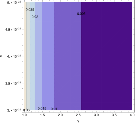
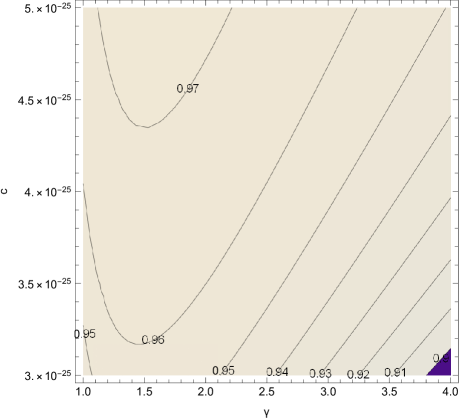
Figure 1: Contour plots of the tensor-to-scalar ratio $r$ (left plot) and the spectral index $n_{\mathcal{S}}$ (right plot) depending on parameters $c$ and $\gamma$. Their values range from [$3\times 10^{-25}$,$5\times 10^{-25}$] and [1,4] for $c$ and $\gamma$ respectively.

This is exactly why the error function was chosen in the first place. In consequence, we can evaluate the final value of the scalar field by letting slow-roll index $\epsilon_{1}$ in Eq. (40) become equal to unity. Doing so, we end up with two values for the scalar field,

$$\centering\phi_{f}=\pm\frac{\sqrt{\omega}}{2\sqrt{2}\kappa\gamma^{2}}\,,\@add@centering$$ (45)

Hence, recalling the $e$-foldings number formula in Eq. (35) and using the previous result, the initial value of the scalar field at the first horizon crossing reads,

$$\phi_{i}=\pm\frac{\sqrt{8N\gamma^{2}+\omega}}{2\sqrt{2}\kappa\gamma^{2}}\,,$$ (46)

Each value of the scalar field is given by two signs, either a plus or a minus, but we keep the physically consistent value, which is the positive of course. For simplicity, we shall use the reduced Planck physical units system, for which $\kappa^{2}=1$. Assuming that the free parameters have the following values ($\omega$, $y_{0}$, $\gamma$, $c$)=(1, 1, 2, 4.09413$\times 10^{-25}$) in reduced Planck units, meaning $\kappa=1$, the spectral indices and the tensor-to-scalar ratio become equal to $n_{\mathcal{S}}=0.966$, $n_{T}=-0.00342555$ and $r=0.00832892$, which are compatible with the latest Planck data Akrami:2018odb of Eq. (36), at least when the tensor-to-scalar ratio and the spectral index of scalar curvature are considered. The maximum bound for the tensor spectral index coming from Planck 2018 Akrami:2018odb is $n_{T}\simeq 2$ so the present model is also compatible with this constraint, however the tensor tilt coming from the Planck data is strongly related to the minimally coupled canonical scalar field consistency relation assumption, so it is conceivable that the gravity of the tensor tilt $n_{T}$ result cannot be taken into account as seriously as the spectral index and the tensor-to-scalar ratio. Furthermore, the value of the sound speed for the above values of the parameters is $c_{A}^{2}\simeq 0.999994$, so the theory is free from instabilities. Additionally, the values of the scalar field are $\phi_{i}=3.87399$ and $\phi_{f}=0.0883883$ and due to continuity, in can easily be inferred that the value of the scalar field decreases with time.

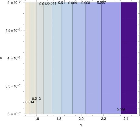
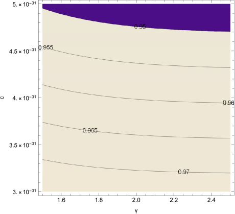
Figure 2: Contour plots of the tensor-to-scalar ratio r (left) and the spectral index $n_{\mathcal{S}}$ (right) depending on parameters $c$ and $\gamma$. Their values range from [$3\times 10^{-31}$,$5\times 10^{-31}$] and [1.5,2.5] for $c$ and $\gamma$ respectively.

It is worth mentioning that this particular set of parameters is not the only one capable of producing viable inflation. It turns out that there exist four different values for the integration constant $c$ which yield the same values for the observed quantities by keeping the rest parameters fixed. Apart from the one used previously, inserting either one from the values in reduced Planck units $c=-4.07962\times 10^{-25}$, $c=3.52933\times 10^{-31}$ or $c=4.72821\times 10^{-28}$ produces the exact same result, implying that there exist more possible values, therefore multiple viable parameter values regions which could produce viable inflation. The following plots depict such regions of viability for the parameters $c$ and $\gamma$. It is obvious from Fig. 1 and Fig. 2 that $\gamma$ affects mainly the spectral index $n_{\mathcal{S}}$ while $c$ both the spectral index and the tensor-to-scalar ratio. For the sake of consistency, we mention that the choice for such small integration constant in Planck-Units is in a way mandatory in order to achieve compatibility with the Planck 2018 data and not a aimed choice of ours. In fact, since the rest free parameters obtained such values, the integration constant essentially was forced to obtain such a small value.

Lastly, we must check whether our approximations we made in the previous section are valid, for the values of the free parameters for which the viability of the model when compared to the Planck data is ensured. By choosing ($\omega$, $y_{0}$, $\gamma$, $c$)=(1, 1, 2, 4.09413$\times 10^{-25}$) in reduced Planck units, we have that $\frac{\dot{H}}{H^{2}}\sim\mathcal{O}(10^{-3})$, so the slow-roll condition (6) holds true. Similarly, the kinetic term at the same epoch is of order $\frac{1}{2}\omega\dot{\phi}^{2}\sim\mathcal{O}(10^{20})$ while the scalar potential is V($\phi$)$\sim\mathcal{O}(10^{24})$, therefore, the slow-roll approximation for the scalar field (10) holds also true. In addition, let us check the condition (13), namely, $12\frac{\xi^{\prime 2}H^{4}}{\xi^{\prime\prime}}\ll V$, so for ($\omega$, $y_{0}$, $\gamma$, $c$)=(1, 1, 2, 4.09413$\times 10^{-25}$), the fraction of the two terms, namely $\frac{12\frac{\xi^{\prime 2}H^{4}}{\xi^{\prime\prime}}}{V}$, is approximately $\frac{12\frac{\xi^{\prime 2}H^{4}}{\xi^{\prime\prime}}}{V}\sim\mathcal{O}(2\times 10^{-3})$, so the approximation is valid in this case too. In conclusion, the error function choice for the scalar Gauss-Bonnet coupling $\xi(\phi)$, yields a phenomenologically viable inflationary era for the GW170817-compatible Einstein-Gauss-Bonnet model.

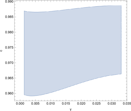
Figure 3: Parametric plot of the tensor-to-scalar ratio r (x axis) and the spectral index $n_{\mathcal{S}}$ (y axis) depending on parameters $c$ and $\gamma$. Their values range from [$2\times 10^{-31}$,$4\times 10^{-31}$] and [1,5] for $c$ and $\gamma$ respectively.

Finally, it is easy to check that all the slow-roll indices satisfy the relation $\epsilon_{i}\ll 1$, $i=1,2,4,5,6$. Indeed, for ($\omega$, $y_{0}$, $\gamma$, $c$)=(1, 1, 2, 4.09413$\times 10^{-25}$) we have $\epsilon_{1}\simeq 0.000520562$, $\epsilon_{2}\simeq 0.00780843$, $\epsilon_{4}\simeq 0.00814159$, $\epsilon_{5}\simeq 0.00119194$ and $\epsilon_{6}\simeq-2.96645\times 10^{-25}$ at the first horizon crossing. Thus, this verifies that the slow-roll condition indeed holds true.

Let us note here that the parameter $c$ has an extremely small value compared to the rest free parameters of the model, even in Planck units. This choice however was made in order to extract a viable phenomenology for the specific model at hand namely model (37). In an essence, our analysis showed that the parameter $c$ is forced to take such small and fine-tuned values, in order for the rest of the parameters to have less fine-tuned values, and simultaneously in order to obtain a viable phenomenology. Perhaps, a complete different designation of the free parameters value could lead to a viable phenomenology, without such extreme fine-tuning on the parameter $c$. This case is a possibility however we refrained from further analysis the parameter space, because the model itself is just a choice made for demonstrative reasons. It is obvious that a more refined model would require less fine-tuning to the free parameters, and as we show in the next sections, this is indeed the case.

III.2 Phenomenology of a More Involved Model

Suppose now that the Gauss-Bonnet coupling scalar function has the following form,

$$\centering\xi(\phi)=\int^{\phi}{y_{1}e^{-\delta(\kappa\tau)^{n}}d\tau}\,,\@add@centering$$ (47)

where $y_{1}$, $\delta$ and $n$ are dimensionless constants to be specified later. As it was the case with the previous model, the second derivative of the coupling function is connected with the first via a generalized equation compared to the first model,

$$\centering\xi^{\prime\prime}=-n\delta\kappa^{n}\phi^{n-1}\xi^{\prime}\,.\@add@centering$$ (48)

Thus, both the slow-roll indices $\epsilon_{1}$ and $\epsilon_{2}$, the $e$-foldings number $N$ and the derivative of the scalar field $\dot{\phi}$ are given again by simple expressions which are proportional to the exponent $n$ of the model function (47). Consequently, specifying the exponent should in principle produce expressions for the observable quantities depending strongly on the exponent. On the other hand, the scalar potential derived from Eq.(17) has a complicated form, as is shown below,

$$\centering V(\phi)=\frac{e^{\frac{\omega(\kappa\phi)^{3-n}}{(3-n)\delta n}}}{\int_{1}^{\phi}\frac{4}{3}\kappa^{4}y_{1}e^{\frac{k^{3-n}\omega\tau^{3-n}}{(3-n)\delta n}-\delta\kappa^{n}\tau^{n}}\,d\tau}\,,\@add@centering$$ (49)

and $\tau$ an auxiliary integration variable. Moreover, the arbitrary constant derived from the integration is assumed to be equal to zero. However, the scalar potential enters only in the equations through the Hubble rate, so it will affect only the rest of the slow-roll indices and the observable quantities as well. Since the scalar potential is also depending on the exponent of the Gauss-Bonnet scalar function, the dominant factor which in the end shall determine the viability of the model is this exponent. Let us now proceed with the evaluation of the slow-roll indices. Recalling their previous definitions in Eq. (24) through Eq. (26) and the coupling function $\xi(\phi)$ in Eq. (47) as well, we end up with the following formulas.

$$\centering\epsilon_{1}\simeq\frac{\omega}{2}\left(\frac{1}{n\delta(\kappa\phi)^{n-1}}\right)^{2}\,,\@add@centering$$ (50)

$$\centering\epsilon_{2}\simeq\frac{(n-1)}{n\delta(\kappa\phi)^{n}}-\epsilon_{1}\,,\@add@centering$$ (51)

$$\centering\epsilon_{3}=0\,,\@add@centering$$ (52)

Apparently, the first three slow-roll indices have very simple forms, while the rest were omitted due to their lengthy final forms. Note however that the indices $\epsilon_{4}$ and $\epsilon_{6}$ participate in the evaluation of the spectral indices and the tensor-to-scalar ratio directly. The values of both the spectral indices and the tensor-to-scalar ratio, as mentioned before, can be calculated by utilizing the slow-roll indices introduced previously. Similarly, from Eq. (50), the value of the scalar field at the end of inflation can be derived by equating the index $\epsilon_{1}$ with unity. Thus, the final value of the scalar field in this case is,

$$\centering\phi_{f}=\frac{1}{\kappa}\left(\frac{1}{\delta n}\sqrt{\frac{\omega}{2}}\right)^{\frac{1}{n-1}}\,,\@add@centering$$ (53)

Similarly, the initial value of the scalar field at the first horizon crossing can be inferred from the final value and the $e$-foldings number in Eq. (35) by simply solving the integral. Thus, the initial value is,

$$\centering\phi_{i}=\frac{1}{\kappa}\left(\left(\frac{1}{n\delta}\sqrt{\frac{\omega}{2}}\right)^{\frac{n}{n-1}}+\frac{N}{\delta}\right)^{\frac{1}{n}}\,,\@add@centering$$ (54)

where $N\simeq 60$. An observant reader might notice that the two previous results are presented in an incomplete manner, since the expression of the final value of the scalar field should produce at least $2n-2$ solutions while the initial value, only $n$. Mathematically speaking, that would be correct, however, in order to avoid the emergence of complex numbers, it was deemed necessary to choose the positive value in each case. These values in fact will lead to a viable model while the rest are physically inconsistent. Hence, the positive value at the initial stage of inflation shall be used as input in the spectral index and tensor-to-scalar ratio in order to calculate the observable quantities and ascertain the validity of the model by comparing them with the values obtained by the Planck 2018 collaboration Akrami:2018odb . Let us assume that in Planck Units, in reduced Planck units with $\kappa^{2}=1$, the free parameters of the theory have the following fixed values, ($\omega$, $y_{1}$, $\delta$, n)=(1, 0.0001, 3.33, 100). According to the previous results for the scalar field in Eq. (54) and Eq. (53), the initial and final value of the scalar field becomes equal to $\phi_{i}=1.02933$ and $\phi_{f}=0.939715$ respectively in Planck Units. At first site, it is clear that the scalar field again decreases with time. Consequently, the observable quantities take the values $n_{\mathcal{S}}=0.967004$, and $r=2.35395\times 10^{-7}$, which are both compatible with latest Planck observations (36) and the unobserved for now spectral index of the tensor perturbations is equal to $n_{T}=-2.94244\times 10^{-8}$, which is incompatible with the upper bound of the Planck data $n_{T}\sim 2$ Akrami:2018odb , but still the Planck result depends strongly on the consistency relation for a minimally coupled canonical scalar theory. Generally speaking, the previous results were obtained for specific values of the free parameters and especially, for a fixed value of the exponent $n$ in Eq. (47). However, this is not the only set of parameters capable of producing compatible results with the observations. It seems that each parameter is insignificant compared to the exponent $n$, with the latter having a dominant effect on the phenomenology produced. However, there is a wide range of values of the parameter $n$, which may range from [15,120] and even further, and as $n$ increases, both the spectral index of primordial curvature perturbations $n_{\mathcal{S}}$ and the tensor-to-scalar ratio $r$ decrease, but at different rates. Specifically, the rate of decrease for the spectral index is lesser than the rate of decrease for the tensor-to-scalar ratio. Since there exists no lower boundary for the latter, there exists a wide range of possible values for the exponent $n$ as is shown in Fig. 4 and Fig. 5. In the plots we present two cases for which the viability of the model is achieved as mentioned before. Parameters $1/\delta$, for convenience, and $n$ were chosen to study the response of the model in such changes. In contrast to the previous model, it seems that now, the tensor-to-scalar ratio depends on $\delta$ while the spectral index remains unaffected. In addition, the exponent as expected affects strongly both quantities.

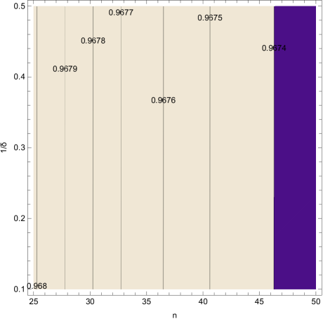
Figure 4: Contour plots of the tensor-to-scalar ratio $r$ (left) and the spectral index $n_{\mathcal{S}}$ (right) depending on the dimensionless parameters $1/\delta$ and $n$. Their values range from [$0.1$,$0.5$] and [25,50] for $1/\delta$ and $n$ respectively.

Lastly, we discuss the validity of the approximations made throughout our calculations. Firstly, the slow-roll condition for the scalar field (10), so by choosing ($\omega$, $y_{1}$, $\delta$, n)=(1, 0.0001, 3.33, 100) in our case we have, $\frac{1}{2}\omega\dot{\phi}^{2}\sim\mathcal{O}(10^{-5})$ while $V(\phi)\sim\mathcal{O}(10^{4})$ in reduced Planck units, so apparently it holds true. Also, $\dot{H}\sim\mathcal{O}(10^{-5})$ and $H^{2}\sim\mathcal{O}(10^{3})$, and therefore the condition (6) also holds true. Similarly, in the first gravitational equation of motion, the term $\sim\dot{\xi}H^{3}$ was omitted as it was deemed small compared to the value of the scalar potential. This assumption is proven to be true since at the horizon crossing, the order of magnitude of this term is much smaller than the corresponding one for the scalar potential, since $\dot{\xi}H^{3}\sim\mathcal{O}(10^{-31})$, while $V(\phi)\sim\mathcal{O}(10^{4})$ in reduced Planck units at the horizon crossing. Finally, we note that the initial ratio of the first two derivatives of the Gauss-Bonnet coupling scalar function is of order $\xi^{\prime}/\xi^{\prime\prime}\sim\mathcal{O}(10^{-8})$, yet again it is something expected since this ratio is connected with the ratio $\dot{H}/H^{2}$. In the next section we shall further discuss this issue.

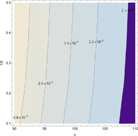
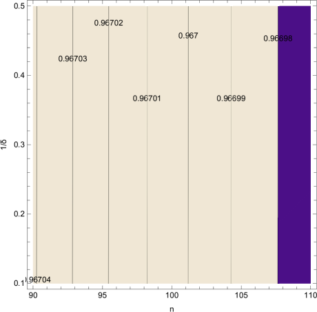
Figure 5: Contour plots of the tensor-to-scalar ratio r (left) and the spectral index $n_{\mathcal{S}}$ (right) depending on the dimensionless parameters $1/\delta$ and $n$. Their values range from [$0.1$,$0.5$] and [90,110] for $1/\delta$ and $n$ respectively.

As a last comment, it is worth mentioning certain similarities, and differences as well, between the two models. Setting $n=2$, $\delta=4$ and $y_{1}=2$, in principle, the models should coincide since the ratio $\xi^{\prime}/\xi^{\prime\prime}$ is exactly the same. Following this research line, the initial and the final values of the scalar field are also the same, something that is expected since it attributed to the previous ratio equivalence. However, since in the second model,the integration constant is zero, in contrast to the first, the scalar potential will be different. Therefore, the indices $\epsilon_{4}$ through $\epsilon_{6}$, the sound wave speed $c_{A}$ and the spectral index $n_{\mathcal{S}}$ as well, are different in each model since these parameters depend on the scalar potential. For the tensor-to-scalar ratio which also depends from the sound wave speed, the result is the same up some accuracy, implying that the dominant factor, which in fact experiences greater change, is the index $\epsilon_{4}$. Despite that, there is no limitation that forbids the two models in agreeing with each other but if that is the case, a different set of parameters is needed. Furthermore, the previous analysis has made it abundantly clear that in order to yield viable results, one can work in two separate ways. Either freeze the exponent $n$ and find an appropriate initial condition for the scalar potential, meaning designating properly the arbitrary integration constant, or neglect this particular constant by equating it with zero, and vary the exponent $n$. Having both the exponent and the integration constant taking values simultaneously is surely a possibility, that in principle could yield viable results, but this issue is a by far more complicated task.

III.3 Phenomenology Under the Assumption $\xi^{\prime}/\xi^{\prime\prime}\ll 1$

Let us consider again the condition $\frac{\dot{\phi}^{2}}{2}\ll V$, which can be rewritten as,

$$\frac{\frac{\dot{\phi}^{2}}{2}}{V}\ll 1\,,$$ (55)

and by using Eq. (16), we can write Eq. (55) as follows,

$$\frac{\kappa^{2}}{6}\frac{\xi^{\prime 2}}{\xi^{\prime\prime 2}}\ll 1\,.$$ (56)

It is rather tempting to investigate the phenomenology of the GW170817-compatible Einstein-Gauss-Bonnet model in the case that the following additional condition holds true,

$$\kappa\frac{\xi^{\prime}}{\xi^{\prime\prime}}\ll 1\,,$$ (57)

which is motivated from the condition $\frac{\xi^{\prime 2}\kappa^{2}}{6\xi^{\prime\prime 2}}\ll 1$ of Eq. (56). In this case, in view of the constraint (57) the term $\frac{\xi^{\prime}}{\xi^{\prime\prime}}$ can be disregarded in Eq. (17), so the latter becomes,

$$\centering\frac{V^{\prime}}{V}+\frac{4}{3}\xi^{\prime}V\kappa^{4}\simeq 0\,.\@add@centering$$ (58)

This means that the two terms $\sim\frac{V^{\prime}}{V}$ and $\sim\xi^{\prime}V$ are of the same order in Planck units. Also, it is obvious that in the case at hand, the differential equation (58) that yields the scalar potential, for a given function $\xi(\phi)$, or vice versa, is more easy to solve analytically. Another motivation for choosing the condition (57) is the fact that the first slow-roll index $\epsilon_{1}$ in Eq. (24) is proportional to the ratio $\left(\xi^{\prime}/\xi^{\prime\prime}\right)^{2}$ and the value of such index at the first horizon crossing is expected to be much lesser than unity, if the slow-roll conditions apply in the theory. Thus, it stands to reason why this ratio can be neglected.

In this section, we shall investigate the phenomenological implications of the condition (57) on the GW170817-compatible Einstein-Gauss-Bonnet theory. What will actually change in the whole procedure we developed in the previous section, is the relation that gives the scalar potential $V(\phi)$ given the scalar coupling function $\xi(\phi)$ and vice versa. The relations that yield the slow-roll indices as functions of the scalar field and the corresponding observational indices remain the same, so effectively we have a simpler theoretical framework. Let us demonstrate how the phenomenology of the GW170817-compatible Einstein-Gauss-Bonnet theory is modified in view of the assumption (58). In the following, we shall examine three simple models and explicitly confront the models whether they lead to viable results or inconsistencies.

Suppose first that the coupling function is given by a simple power-law scalar field dependence,

$$\centering\xi(\phi)=\lambda(\kappa\phi)^{m}\,,\@add@centering$$ (59)

were $\lambda$ is a dimensionless constant. This particular model also belongs to the same category as the previous ones, since there exists a simple connection between the derivatives of $\xi(\phi)$. Specifically,

$$\centering\xi^{\prime\prime}=\frac{(m-1)}{\phi}\xi^{\prime}\,,\@add@centering$$ (60)

so accordingly, the slow-roll indices $\epsilon_{1},\epsilon_{2}$, the $e$-foldings number relation and the initial-final value of the scalar field, are given by simple expressions. Following the same procedure as in the previous section, the scalar potential can be extracted from Eq. (58), which reads,

$$\centering V(\phi)=\frac{1}{\frac{4}{3}\kappa^{4}\xi(\phi)-c_{1}}\,,\@add@centering$$ (61)

where $c_{1}$ is an arbitrary integration constant with mass dimensions [m]^-4. This is a much simpler expression for the scalar potential compared to the models of the previous sections. Now we shall examine the viability of the power-law model where the arbitrary integration constant in non-zero and accordingly we shall examine the case when this particular constant is in fact equal to zero. The latter is a very interesting case since as it can be inferred from Eq. (61), the product of the scalar potential and the Gauss-Bonnet coupling scalar function is a well defined constant, and as a matter of fact, one with very restricted form, as it can be inferred by Eq. (58). Let us proceed with the first case where the the integration constant is nonzero. Then, similar to the previous two models, the slow-roll indices derived from Eqs. (24)-(29) have the following form,

$$\centering\epsilon_{1}\simeq\frac{\omega(\kappa\phi)^{2}}{2(m-1)^{2}}\,,\@add@centering$$ (62)

$$\centering\epsilon_{2}\simeq-\frac{\omega(\kappa\phi)^{2}-2m+2}{2(m-1)^{2}}\,,\@add@centering$$ (63)

$$\centering\epsilon_{3}=0\,,\@add@centering$$ (64)

$$\centering\epsilon_{5}\simeq\frac{2\kappa^{4}\lambda m(\kappa\phi)^{m}}{3c_{1}(m-1)+4\kappa^{4}\lambda(\kappa\phi)^{m}}\,,\@add@centering$$ (65)

$$\centering\epsilon_{6}\simeq\frac{\kappa^{4}\lambda m(\kappa\phi)^{m}\left(-\omega(\kappa\phi)^{2}+2(m-1)^{2}\right)}{(m-1)^{2}\left(3c_{1}(m-1)+4\kappa^{4}\lambda(\kappa\phi)^{m}\right)}\,.\@add@centering$$ (66)

For this model, the slow-roll indices have a particularly simple form, apart from $\epsilon_{4}$, which was yet again omitted due to its perplexed form. Continuing with our calculations, the initial and the final value of the scalar field are extracted from Eq. (35) and Eq. (62) respectively are,

$$\centering\phi_{f}=\frac{|m-1|}{\kappa}\sqrt{\frac{2}{\omega}}\,,\@add@centering$$ (67)

$$\centering\phi_{i}=\frac{|m-1|e^{-\frac{N}{m-1}}}{\kappa}\sqrt{\frac{2}{\omega}}\,.\@add@centering$$ (68)

Choosing appropriately the free parameters of the model, it can yield compatible results with the observations. Assuming for example that ($\omega$, $\lambda$, $m$, $c_{1}$) are equal to (1, 1, 12, 4.4512$\times 10^{-15}$) in reduced Planck units, viable results are produced, since the values $n_{\mathcal{S}}=0.965$ for the spectral index of primordial curvature perturbations and $r=0.00029265$ for the tensor-to-scalar ratio are both accepted values. In addition, the spectral index of tensor modes is equal to $n_{T}=-0.00003658$ which as expected has a very small value. Similarly, the values of the scalar field from Eq. (68) and Eq. (67) are $\phi_{i}=0.665317$ and $\phi_{f}=15.5563$ in Planck Units. In this case, the scalar field increases as time flows, in contrast to the models of the previous section.

Lastly, we note that all the approximations made in this power-law model, both the slow-roll approximations and the ratio $\xi^{\prime}/\xi^{\prime\prime}$ hold true. We note that at the start of inflation the slow-roll approximation seems valid, since $\dot{H}/H^{2}\sim\mathcal{O}(10^{-4})$ and the kinetic term of the scalar field as well is insignificant compared to the scalar potential as $\frac{1}{2}\omega\dot{\phi}^{2}\sim\mathcal{O}(10^{9})$ and $V(\phi)\sim\mathcal{O}(10^{14})$. Finally, the condition (57) must also be investigated if it holds true, so by choosing $(\omega,\lambda,m,c_{1})=(1,1,12,4.4512\times 10^{-15})$ we have, $V^{\prime}/V\sim\mathcal{O}(10^{3})$, $\xi^{\prime}V\sim\mathcal{O}(10^{3})$ while $\xi^{\prime}/\xi^{\prime\prime}\sim\mathcal{O}(10^{-3})$. Thus the term $\xi^{\prime}/\xi^{\prime\prime}$ is indeed insignificant compared to the other terms entering the differential equation (17).

Now let us proceed to some examples for which the viability with the observational data cannot be achieved. Let us now examine the case where,

$$\centering\xi(\phi)V(\phi)=\Lambda\,,\@add@centering$$ (69)

This assumption simplifies again Eq. (58) which now reads

$$\centering V^{\prime}(\phi)(1-\Lambda\frac{4}{3}\kappa^{4})=0\,,\@add@centering$$ (70)

This particular differential equation can be interpreted in two ways. Either the expression in the parenthesis is zero, meaning that $\Lambda=\frac{3}{4\kappa^{4}}$, which is equivalent to the previous case with $c_{1}=0$, or the derivative of the scalar potential is equal to zero. The latter case requires that the coupling function is also independent of $\phi$, so in this case we are lead to physical inconsistencies, since the expressions proportional to the ratio $\xi^{\prime}/\xi^{\prime\prime}$ cannot be defined. Thus, the only reasonable explanation is to assume the same power-law model and demand that the integration constant is exactly zero. Consequently,

$$\centering\xi(\phi)=\lambda(\kappa\phi)^{m}\,,\@add@centering$$ (71)

$$\centering V(\phi)=\frac{\Lambda}{\xi(\phi)}\,,\@add@centering$$ (72)

As a result, the equations for the slow-roll indices and the expressions for the values of the scalar field at the start and the end of inflation remain the same, where now $c_{1}=0$ in slow-roll indices $\epsilon_{5}$ and $\epsilon_{6}$, and so we can proceed directly with the evaluation of the observed quantities, by designating properly the free parameters. However we must keep in mind that now, the number of free parameters is reduced by one, since Eq. (70) demands that $\Lambda\frac{4}{3}\kappa^{4}=1$. Unfortunately, there exists no proper set of parameters which can lead to viability. It turns out that compatibility may be achieved, only if the arbitrary integration constant $c_{1}$ derived from Eq. (61) has a non-zero value.

Let us briefly discuss another model, in which is related to the string motivated Einstein-dilaton gravity, in which case the coupling scalar function now is defined as,

$$\centering\xi(\phi)=Ye^{\alpha(\kappa\phi)}\,.\@add@centering$$ (73)

In this case, we shall not derive the formula for the scalar potential but we shall work only with the first slow-roll index from Eq. (24). Subsequently, this particular index has the following form,

$$\centering\epsilon_{1}\simeq\frac{\omega}{2\alpha^{2}}\,,\@add@centering$$ (74)

It turns out that $\epsilon_{1}$ is $\phi$ independent, therefore, it is certain that this model leads to eternal inflation, if $\alpha\gg 1$, or to no inflation at all if $\alpha\ll 1$, like the canonical scalar theory case with exponential potential. However, if $\alpha\gg 1$, it may be that the first slow-roll index and the second one, as it can be shown, are constants, but the slow-roll indices $\epsilon_{4}$, $\epsilon_{5}$ and $\epsilon_{6}$ are $\phi$-dependent. Thus, it may be possible that one may assume that the inflationary era might end when one of these acquires values of the order $\sim\mathcal{O}(1)$. This is a possibility, but we shall not further pursuit this issue here.

Before ending, let us comment on an interesting issue related to the Swampland criteria Vafa:2005ui ; Ooguri:2006in ; Palti:2020qlc ; Brandenberger:2020oav ; Blumenhagen:2019vgj ; Wang:2019eym ; Benetti:2019smr ; Palti:2019pca ; Cai:2018ebs ; Mizuno:2019pcm ; Aragam:2019khr ; Brahma:2019mdd ; Mukhopadhyay:2019cai ; Marsh:2019lhu ; Brahma:2019kch ; Haque:2019prw ; Heckman:2019dsj ; Acharya:2018deu ; Cheong:2018udx ; Heckman:2018mxl ; Lin:2018rnx ; Park:2018fuj ; Olguin-Tejo:2018pfq ; Fukuda:2018haz ; Wang:2018kly ; Ooguri:2018wrx ; Matsui:2018xwa ; Obied:2018sgi ; Agrawal:2018own ; Murayama:2018lie ; Marsh:2018kub in the context of Einstein-Gauss-Bonnet theory. This was developed in Ref. Yi:2018dhl , and as it was shown, the Swampland criteria can hold true, if the scalar Gauss-Bonnet coupling is chosen as,

$$\xi(\phi)=\frac{C}{V(\phi)}\,,$$ (75)

however in our case, where we take the GW170817 constraints into account, the coupling function $\xi(\phi)$ of Eq. (75) does not satisfy the differential equation (17), unless the potential has a very specific form, which is the following,

$$V(\phi)=A\sec\left[\frac{\kappa\sqrt{\omega}\left(B\left(4\kappa^{4}C-3\right)+\phi\right)}{\sqrt{\frac{4}{3}\kappa^{4}C-1}}\right]\,,$$ (76)

where $A$ and $B$ are integration constants. As it can be shown, the above potential does not yield a viable phenomenology though. In addition, if we assume that the additional condition (57) holds true, then it can be shown that the coupling function $\xi(\phi)$ of Eq. (75) can satisfy the corresponding differential equation (58) only if $C=\frac{3}{4\kappa^{4}}$, however in this scenario too the model is not a viable inflationary model, as we showed earlier in this section (see Eq. (69)), since it leads to incompatible observational indices with the observational data of Planck. Nevertheless, in Ref. PhysicsLetters , we shall demonstrate that the Swampland criteria are naturally satisfied in the context of the GW170817 Einstein-Gauss-Bonnet theory, for general choices of the scalar coupling function $\xi(\phi)$ and of the potential $V(\phi)$.

IV Conclusions

In this work we introduced a new theoretical framework for studying Einstein-Gauss-Bonnet theories of gravity, which results to particularly elegant and functionally simple gravitational equations of motion, slow-roll indices and observational indices. Particularly, by requiring the Einstein-Gauss-Bonnet theory to be compatible with the GW170817 event, we ended up with a constraint on the functional forms that the scalar Gauss-Bonnet coupling function $\xi(\phi)$ and the scalar potential $V(\phi)$ must have. By also using the slow-roll assumption for the scalar field and the Hubble rate, we demonstrated that the gravitational equations of motion end up to have a very simple form, and that the scalar Gauss-Bonnet coupling function $\xi(\phi)$ and the scalar potential $V(\phi)$ must satisfy a differential equation. Accordingly we calculated the slow-roll indices for the GW170817-compatible Einstein-Gauss-Bonnet theory, and we calculated the observational indices of inflation too. With regard to the latter, we focused on the spectral indices of scalar and tensor perturbations and the tensor-to-scalar ratio. We applied the formalism we derived in several models of interest, and we confronted the models directly with the observational data coming from the latest Planck 2018 results. Particularly, the most interesting model has a scalar Gauss-Bonnet coupling function $\xi(\phi)$ related to the error function. As we showed, this model and a generalized model based on this, is compatible with the Planck 2018 data, for a wide range of the free parameters values. In addition, all the models we presented satisfy all the constraints imposed by the slow-roll and additional assumptions, made for the derivation of the gravitational equations of motion.

More interestingly, we investigated the phenomenological implications of the additional condition $\xi^{\prime}/\xi^{\prime\prime}\ll 1$, which is motivated by the slow-roll conditions that are assumed to hold true. As it turns, the resulting differential equation that constrains the functional form of the scalar Gauss-Bonnet coupling function $\xi(\phi)$ and of the scalar potential $V(\phi)$, becomes simpler in this case, and this opened a new window for obtaining interesting inflationary phenomenology. We presented three models of interest, in all of which we fixed the scalar Gauss-Bonnet coupling function $\xi(\phi)$ to be a power-law type, exponential and of the form $\xi(\phi)\sim 1/V(\phi)$. The power-law type of model was demonstrated to be compatible with the observational data, while the last two were found incompatible with the observational data. We also further discussed in brief the case $\xi(\phi)\sim 1/V(\phi)$ which is related to the Swampland in the context of Einstein-Gauss-Bonnet theories. As we showed, the functional form $\xi(\phi)\sim 1/V(\phi)$ is not compatible with the GW170817 results, unless the potential has a very specific form, which however leads to non-viable inflationary phenomenological results. However, as we show in another work PhysicsLetters , the Swampland criteria are compatible with the GW170817-compatible Einstein-Gauss-Bonnet theories for quite general functional forms of the scalar Gauss-Bonnet coupling function $\xi(\phi)$ and of the scalar potential $V(\phi)$.

In principle, more elaborate potentials can also produce quite interesting phenomenology in the context of the GW170817-compatible Einstein-Gauss-Bonnet theories, by simply fixing the scalar potential and seeking for the the scalar Gauss-Bonnet coupling function $\xi(\phi)$, or vice-versa. However, this paper was an introductory paper introducing the new formalism, and showing that it is possible to provide phenomenologically viable results for the inflationary era. We hope in a future work to provide further interesting models that yields also a phenomenologically viable inflationary era.

Another interesting question we would like to comment on before closing is whether Einstein-Gauss-Bonnet theories can in principle be reduced to Einstein’s General Relativity in some limit. It is possible to obtain Einstein gravity in the presence of a scalar field during some eras in a cosmological context, if the scalar coupling function $\xi(\phi)$ takes values in that era quite small or nearly constant, and only if the curvature during that era is very small. In the case of small values the scalar-Gauss-Bonnet term can be small, and if $\xi(\phi)$ is nearly constant, the Gauss-Bonnet term can be integrated from the action, thus it has no effect, and we are left with Einstein gravity in the presence of a scalar field with potential. Nevertheless, during inflation, where the curvature is quite large this is not possible. This smoothing to the general relativity case can occur only during the late-time era, as was shown in Ref. Nojiri:2005vv , see also references therein.

However, caution is needed when considering these higher order string motivated theories. In general, Einstein-Gauss-Bonnet gravity is one of the two theories that violate the General Relativity requirement that the metric tensor solely mediates gravity Nair:2019iur , the other theory is the four dimensional Chern-Simons gravity, that is, a gravitational theory with again the presence of a coupling between the scalar field and the four dimensional Chern-Pontryagin term, which is a topological invariant in four dimensions, but in the presence of the scalar field coupling to it, it yields non-trivial effects, like in the Einstein-Gauss-Bonnet case. Both the aforementioned theories are string theory motivated, and can be the low-energy limit of a more fundamental string theory, upon dimensional reduction of the latter.

These theories in general, and particularly the Einstein-Gauss-Bonnet theories, have brought along major differences in astrophysical context. Particularly, the major prediction is that black holes are scalarized (see for example Nair:2019iur ; Carson:2020cqb ), thus a fifth force emerges in these theories, in addition to the violation of the strong equivalence principle. Moreover, higher order effects in binaries are also predicted, like scalar dipole radiation, which in effect makes the rate of an inspiral of a binary system somewhat faster, thus making clear the distinction between general relativity and Einstein-Gauss-Bonnet theories Carson:2020cqb . Thus answering the question whether a smooth limit to Einstein gravity can be obtained, is not easy in general.

References

- (1) A. G. Riess et al. [Supernova Search Team], Astron. J. 116 (1998) 1009 [astro-ph/9805201].
- (2) B. P. Abbott et al. “Multi-messenger Observations of a Binary Neutron Star Merger,” Astrophys. J. 848 (2017) no.2, L12 doi:10.3847/2041-8213/aa91c9 [arXiv:1710.05833 [astro-ph.HE]].
- (3) J. M. Ezquiaga and M. Zumalacarregui, Phys. Rev. Lett. 119 (2017) no.25, 251304 doi:10.1103/PhysRevLett.119.251304 [arXiv:1710.05901 [astro-ph.CO]].
- (4) S. D. Odintsov and V. K. Oikonomou, Phys. Lett. B 797 (2019) 134874 doi:10.1016/j.physletb.2019.134874 [arXiv:1908.07555 [gr-qc]].
- (5) J. c. Hwang and H. Noh, Phys. Rev. D 71 (2005) 063536 doi:10.1103/PhysRevD.71.063536 [gr-qc/0412126].
- (6) S. Nojiri, S. D. Odintsov and M. Sami, Phys. Rev. D 74 (2006) 046004 doi:10.1103/PhysRevD.74.046004 [hep-th/0605039].
- (7) G. Cognola, E. Elizalde, S. Nojiri, S. Odintsov and S. Zerbini, Phys. Rev. D 75 (2007) 086002 doi:10.1103/PhysRevD.75.086002 [hep-th/0611198].
- (8) S. Nojiri, S. D. Odintsov and M. Sasaki, Phys. Rev. D 71 (2005) 123509 doi:10.1103/PhysRevD.71.123509 [hep-th/0504052].
- (9) S. Nojiri and S. D. Odintsov, Phys. Lett. B 631 (2005) 1 doi:10.1016/j.physletb.2005.10.010 [hep-th/0508049].
- (10) M. Satoh, S. Kanno and J. Soda, Phys. Rev. D 77 (2008) 023526 doi:10.1103/PhysRevD.77.023526 [arXiv:0706.3585 [astro-ph]].
- (11) K. Bamba, A. N. Makarenko, A. N. Myagky and S. D. Odintsov, JCAP 1504 (2015) 001 doi:10.1088/1475-7516/2015/04/001 [arXiv:1411.3852 [hep-th]].
- (12) Z. Yi, Y. Gong and M. Sabir, Phys. Rev. D 98 (2018) no.8, 083521 doi:10.1103/PhysRevD.98.083521 [arXiv:1804.09116 [gr-qc]].
- (13) Z. K. Guo and D. J. Schwarz, Phys. Rev. D 80 (2009) 063523 doi:10.1103/PhysRevD.80.063523 [arXiv:0907.0427 [hep-th]].
- (14) Z. K. Guo and D. J. Schwarz, Phys. Rev. D 81 (2010) 123520 doi:10.1103/PhysRevD.81.123520 [arXiv:1001.1897 [hep-th]].
- (15) P. X. Jiang, J. W. Hu and Z. K. Guo, Phys. Rev. D 88 (2013) 123508 doi:10.1103/PhysRevD.88.123508 [arXiv:1310.5579 [hep-th]].
- (16) P. Kanti, R. Gannouji and N. Dadhich, Phys. Rev. D 92 (2015) no.4, 041302 doi:10.1103/PhysRevD.92.041302 [arXiv:1503.01579 [hep-th]].
- (17) C. van de Bruck, K. Dimopoulos, C. Longden and C. Owen, arXiv:1707.06839 [astro-ph.CO].
- (18) P. Kanti, J. Rizos and K. Tamvakis, Phys. Rev. D 59 (1999) 083512 doi:10.1103/PhysRevD.59.083512 [gr-qc/9806085].
- (19) S. Kawai and J. Soda, Phys. Lett. B 460 (1999) 41 doi:10.1016/S0370-2693(99)00736-4 [gr-qc/9903017].
- (20) K. Nozari and N. Rashidi, Phys. Rev. D 95 (2017) no.12, 123518 doi:10.1103/PhysRevD.95.123518 [arXiv:1705.02617 [astro-ph.CO]].
- (21) S. Chakraborty, T. Paul and S. SenGupta, Phys. Rev. D 98 (2018) no.8, 083539 doi:10.1103/PhysRevD.98.083539 [arXiv:1804.03004 [gr-qc]].
- (22) S. D. Odintsov and V. K. Oikonomou, Phys. Rev. D 98 (2018) no.4, 044039 doi:10.1103/PhysRevD.98.044039 [arXiv:1808.05045 [gr-qc]].
- (23) S. Kawai, M. a. Sakagami and J. Soda, Phys. Lett. B 437, 284 (1998) doi:10.1016/S0370-2693(98)00925-3 [gr-qc/9802033].
- (24) Z. Yi and Y. Gong, Universe 5 (2019) no.9, 200 doi:10.3390/universe5090200 [arXiv:1811.01625 [gr-qc]].
- (25) C. van de Bruck, K. Dimopoulos and C. Longden, Phys. Rev. D 94 (2016) no.2, 023506 doi:10.1103/PhysRevD.94.023506 [arXiv:1605.06350 [astro-ph.CO]].
- (26) B. Kleihaus, J. Kunz and P. Kanti, arXiv:1910.02121 [gr-qc].
- (27) A. Bakopoulos, P. Kanti and N. Pappas, Phys. Rev. D 101 (2020) no.4, 044026 doi:10.1103/PhysRevD.101.044026 [arXiv:1910.14637 [hep-th]].
- (28) K. i. Maeda, N. Ohta and R. Wakebe, Eur. Phys. J. C 72 (2012) 1949 doi:10.1140/epjc/s10052-012-1949-6 [arXiv:1111.3251 [hep-th]].
- (29) A. Bakopoulos, P. Kanti and N. Pappas, arXiv:2003.02473 [hep-th].
- (30) W. Ai, [arXiv:2004.02858 [gr-qc]].
- (31) R. Easther and K. i. Maeda, Phys. Rev. D 54 (1996) 7252 doi:10.1103/PhysRevD.54.7252 [hep-th/9605173].
- (32) I. Antoniadis, J. Rizos and K. Tamvakis, Nucl. Phys. B 415 (1994) 497 doi:10.1016/0550-3213(94)90120-1 [hep-th/9305025].
- (33) I. Antoniadis, C. Bachas, J. R. Ellis and D. V. Nanopoulos, Phys. Lett. B 257 (1991), 278-284 doi:10.1016/0370-2693(91)91893-Z
- (34) P. Kanti, N. Mavromatos, J. Rizos, K. Tamvakis and E. Winstanley, Phys. Rev. D 54 (1996), 5049-5058 doi:10.1103/PhysRevD.54.5049 [arXiv:hep-th/9511071 [hep-th]].
- (35) P. Kanti, N. Mavromatos, J. Rizos, K. Tamvakis and E. Winstanley, Phys. Rev. D 57 (1998), 6255-6264 doi:10.1103/PhysRevD.57.6255 [arXiv:hep-th/9703192 [hep-th]].
- (36) S. Nojiri, S. D. Odintsov and V. K. Oikonomou, Phys. Rept. 692 (2017) 1 doi:10.1016/j.physrep.2017.06.001 [arXiv:1705.11098 [gr-qc]].
- (37) S. Nojiri and S. D. Odintsov, Phys. Rept. 505 (2011) 59 doi:10.1016/j.physrep.2011.04.001 [arXiv:1011.0544 [gr-qc]].
- (38) S. Nojiri and S. D. Odintsov, eConf C 0602061 (2006) 06 [Int. J. Geom. Meth. Mod. Phys. 4 (2007) 115] doi:10.1142/S0219887807001928 [hep-th/0601213].
- (39) S. Capozziello and M. De Laurentis, Phys. Rept. 509 (2011) 167 doi:10.1016/j.physrep.2011.09.003 [arXiv:1108.6266 [gr-qc]].
- (40) V. Faraoni and S. Capozziello, Fundam. Theor. Phys. 170 (2010). doi:10.1007/978-94-007-0165-6
- (41) A. de la Cruz-Dombriz and D. Saez-Gomez, Entropy 14 (2012) 1717 doi:10.3390/e14091717 [arXiv:1207.2663 [gr-qc]].
- (42) G. J. Olmo, Int. J. Mod. Phys. D 20 (2011) 413 doi:10.1142/S0218271811018925 [arXiv:1101.3864 [gr-qc]].
- (43) Y. Akrami et al. [Planck Collaboration], arXiv:1807.06211 [astro-ph.CO].
- (44) C. Vafa, hep-th/0509212.
- (45) H. Ooguri and C. Vafa, Nucl. Phys. B 766 (2007) 21 doi:10.1016/j.nuclphysb.2006.10.033 [hep-th/0605264].
- (46) E. Palti, C. Vafa and T. Weigand, arXiv:2003.10452 [hep-th].
- (47) R. Brandenberger, V. Kamali and R. O. Ramos, arXiv:2002.04925 [hep-th].
- (48) R. Blumenhagen, M. Brinkmann and A. Makridou, JHEP 2002 (2020) 064 [JHEP 2020 (2020) 064] doi:10.1007/JHEP02(2020)064 [arXiv:1910.10185 [hep-th]].
- (49) Z. Wang, R. Brandenberger and L. Heisenberg, arXiv:1907.08943 [hep-th].
- (50) M. Benetti, S. Capozziello and L. L. Graef, Phys. Rev. D 100 (2019) no.8, 084013 doi:10.1103/PhysRevD.100.084013 [arXiv:1905.05654 [gr-qc]].
- (51) E. Palti, Fortsch. Phys. 67 (2019) no.6, 1900037 doi:10.1002/prop.201900037 [arXiv:1903.06239 [hep-th]].
- (52) R. G. Cai, S. Khimphun, B. H. Lee, S. Sun, G. Tumurtushaa and Y. L. Zhang, Phys. Dark Univ. 26 (2019) 100387 doi:10.1016/j.dark.2019.100387 [arXiv:1812.11105 [hep-th]].
- (53) S. Mizuno, S. Mukohyama, S. Pi and Y. L. Zhang, JCAP 1909 (2019) no.09, 072 doi:10.1088/1475-7516/2019/09/072 [arXiv:1905.10950 [hep-th]].
- (54) V. Aragam, S. Paban and R. Rosati, arXiv:1905.07495 [hep-th].
- (55) S. Brahma and M. W. Hossain, Phys. Rev. D 100 (2019) no.8, 086017 doi:10.1103/PhysRevD.100.086017 [arXiv:1904.05810 [hep-th]].
- (56) U. Mukhopadhyay and D. Majumdar, Phys. Rev. D 100 (2019) no.2, 024006 doi:10.1103/PhysRevD.100.024006 [arXiv:1904.01455 [gr-qc]].
- (57) D. M. C. Marsh and J. E. D. Marsh, arXiv:1903.12643 [hep-th].
- (58) S. Brahma and M. W. Hossain, JHEP 1906 (2019) 070 doi:10.1007/JHEP06(2019)070 [arXiv:1902.11014 [hep-th]].
- (59) M. R. Haque and D. Maity, Phys. Rev. D 99 (2019) no.10, 103534 doi:10.1103/PhysRevD.99.103534 [arXiv:1902.09491 [hep-th]].
- (60) J. J. Heckman, C. Lawrie, L. Lin, J. Sakstein and G. Zoccarato, Fortsch. Phys. 67 (2019) no.11, 1900071 doi:10.1002/prop.201900071 [arXiv:1901.10489 [hep-th]].
- (61) B. S. Acharya, A. Maharana and F. Muia, JHEP 1903 (2019) 048 doi:10.1007/JHEP03(2019)048 [arXiv:1811.10633 [hep-th]].
- (62) D. Y. Cheong, S. M. Lee and S. C. Park, Phys. Lett. B 789 (2019) 336 doi:10.1016/j.physletb.2018.12.046 [arXiv:1811.03622 [hep-ph]].
- (63) J. J. Heckman, C. Lawrie, L. Lin and G. Zoccarato, Fortsch. Phys. 67 (2019) no.10, 1900057 doi:10.1002/prop.201900057 [arXiv:1811.01959 [hep-th]].
- (64) C. M. Lin, Phys. Rev. D 99 (2019) no.2, 023519 doi:10.1103/PhysRevD.99.023519 [arXiv:1810.11992 [astro-ph.CO]].
- (65) S. C. Park, JCAP 1901 (2019) 053 doi:10.1088/1475-7516/2019/01/053 [arXiv:1810.11279 [hep-ph]].
- (66) Y. Olguin-Trejo, S. L. Parameswaran, G. Tasinato and I. Zavala, JCAP 1901 (2019) 031 doi:10.1088/1475-7516/2019/01/031 [arXiv:1810.08634 [hep-th]].
- (67) H. Fukuda, R. Saito, S. Shirai and M. Yamazaki, Phys. Rev. D 99 (2019) no.8, 083520 doi:10.1103/PhysRevD.99.083520 [arXiv:1810.06532 [hep-th]].
- (68) S. J. Wang, Phys. Rev. D 99 (2019) no.2, 023529 doi:10.1103/PhysRevD.99.023529 [arXiv:1810.06445 [hep-th]].
- (69) H. Ooguri, E. Palti, G. Shiu and C. Vafa, Phys. Lett. B 788 (2019) 180 doi:10.1016/j.physletb.2018.11.018 [arXiv:1810.05506 [hep-th]].
- (70) H. Matsui, F. Takahashi and M. Yamada, Phys. Lett. B 789 (2019) 387 doi:10.1016/j.physletb.2018.12.055 [arXiv:1809.07286 [astro-ph.CO]].
- (71) G. Obied, H. Ooguri, L. Spodyneiko and C. Vafa, arXiv:1806.08362 [hep-th].
- (72) P. Agrawal, G. Obied, P. J. Steinhardt and C. Vafa, Phys. Lett. B 784 (2018) 271 doi:10.1016/j.physletb.2018.07.040 [arXiv:1806.09718 [hep-th]].
- (73) H. Murayama, M. Yamazaki and T. T. Yanagida, JHEP 1812 (2018) 032 doi:10.1007/JHEP12(2018)032 [arXiv:1809.00478 [hep-th]].
- (74) M. C. David Marsh, Phys. Lett. B 789 (2019) 639 doi:10.1016/j.physletb.2018.11.001 [arXiv:1809.00726 [hep-th]].
- (75) S. Odintsov and V. Oikonomou, Phys. Lett. B 805 (2020), 135437 doi:10.1016/j.physletb.2020.135437 [arXiv:2004.00479 [gr-qc]].
- (76) R. Nair, S. Perkins, H. O. Silva and N. Yunes, Phys. Rev. Lett. 123 (2019) no.19, 191101 doi:10.1103/PhysRevLett.123.191101 [arXiv:1905.00870 [gr-qc]].
- (77) Z. Carson and K. Yagi, [arXiv:2002.08559 [gr-qc]].