Aspects of spontaneous breaking of conformal invariance in the Fishnet CFT

Abstract:

I will discuss spontaneous conformal symmetry breaking in the strongly $\gamma$-deformed limit of the $\mathcal{N}=4$ supersymmetric Yang-Mills theory known as Fishnet Conformal Field Theory.

1 Intoduction and motivation

This talk   is based on the findings of  [1] written in collaboration with Vladimir Kazakov and Mikhail Shaposhnikov, and concerns the spontaneous breakdown of conformal symmetry in a specific limiting case of the $\gamma$-deformed $\mathcal{N}=4$ supersymmetric Yang-Mills (SYM) theory, the Fishnet CFT (FCFT).

The model was discovered a few years ago by Gurdogan and Kazakov [2] and since then it is being extensively studied [3, 4, 5, 6, 7, 8, 9, 10, 11, 12, 13, 14, 15, 16, 17, 18, 19, 20, 21, 22], although the majority of the considerations concern the phase where the conformal symmetry is not broken. The reasons the FCFT has attracted considerable attention are manyfold. Among others, in the planar $N_{c}\to\infty$ limit, although nonsupersymmetric, the theory is a genuine CFT, it appears to be integrable [2, 23, 3] and in addition it accommodates a rich set of flat directions corresponding to spontaneously broken quantum conformal symmetry [1].

Contrary to what happens if the symmetry is unbroken, on top of nontrivial (i.e. symmetry-breaking) flat vacua, the spectrum of the theory—apart from a massless dilaton—comprises massive particle states. Nevertheless, and in spite of the presence of mass scale(s), the vacuum energy is exactly zero (for instance see [24, 25, 26, 27]). This is due to the stringent constraints that conformal invariance imposes on a system. Specifically, it dictates that the potential be a homogeneous function of the fields. In turn, if there exist nontrivial configurations that extremize the potential, then automatically the vacuum energy of the theory vanishes. In the FCFT this happens naturally, i.e. without resorting to finetunings. In general, such solutions were believed to be present only at specific values of the corresponding coupling(s) for nonsupersymmetric theories.

Apart from a possible “academic” interest on the moduli space of the FCFT—especially in connection with the parent $\mathcal{N}=4$ SYM and its $\gamma$-deformation—the existence of natural flat directions which are not lifted by quantum corrections can be of relevance in particle physics phenomenology too. It is conceivable that some of the features of the FCFT concerning the natural breakdown of quantum scale/conformal symmetry may be universal and be also present in more realistic theories. This may in turn put the cosmological constant problem in a different context. Note that the latter theories may provide the appropriate language to address yet another fine-tuning puzzle of the Standard Model: the gauge hierarchy problem. It has been argued that the smallness of the Higgs mass as compared to the Planck scale may be the consequence of scale/conformal symmetry [62, 32] in combination with no particle thresholds between the electroweak and Planck scales [63, 27], and the presence of nonperturbative gravitational effects operative at very high energies [65, 66, 67, 68].

The paper is organized as follows. A (very) basic overview of the FCFT is given in Sec. 2. Classical and quantum aspects of the symmetry breaking vacua are discussed in Sec. 3. The conclusions are presented in Sec. 4.

2 A crash course on the basics of Fishnet CFT

The starting point of the discussion is the purely scalar sector of the $\gamma$-deformed $\mathcal{N}=4$ SYM Lagrangian (for example cf. [69, 2]) 

$$\mathscr{L}=N_{c}\,\text{tr}\left[\partial_{\mu}\hbox to0.0pt{\hskip 0.47916pt\leavevmode\hbox{\set@color$\overline{\hbox{}}$}\hss}{\leavevmode\hbox{\set@color$\phi$}}_{a}\partial_{\mu}\phi_{a}+g_{YM}^{2}\left(\frac{1}{4}\{\hbox to0.0pt{\hskip 0.47916pt\leavevmode\hbox{\set@color$\overline{\hbox{}}$}\hss}{\leavevmode\hbox{\set@color$\phi$}}_{a},\phi_{a}\}\{\hbox to0.0pt{\hskip 0.47916pt\leavevmode\hbox{\set@color$\overline{\hbox{}}$}\hss}{\leavevmode\hbox{\set@color$\phi$}}_{b},\phi_{b}\}-e^{-i\epsilon_{abc}\gamma_{c}}\hbox to0.0pt{\hskip 0.47916pt\leavevmode\hbox{\set@color$\overline{\hbox{}}$}\hss}{\leavevmode\hbox{\set@color$\phi$}}_{a}\hbox to0.0pt{\hskip 0.47916pt\leavevmode\hbox{\set@color$\overline{\hbox{}}$}\hss}{\leavevmode\hbox{\set@color$\phi$}}_{b}\phi_{a}\phi_{b}\right)\right]\ ,$$ (1)

where the $\phi_{a}$’s are 3 complex scalar (traceless) $N_{c}\times N_{c}$ matrices in the adjoint of $SU(N_{c})$, a bar denotes Hermitian conjugation, $g_{YM}$ is the Yang-Mills coupling, and the $\gamma_{a}$’s are the parameters of the deformation, also called “twists.” In the above, summation over all repeated spacetime $(\mu=0,\ldots,3)$ as well as internal $(a,b,c=1,2,3)$ indexes is tacitly assumed; as customary, the curly brackets stand for the anticommutator and $\epsilon_{abc}$ is the three-dimensional totally antisymmetric symbol. The $\gamma$-deformed theory is defined by (1), supplemented by the corresponding gauge and fermionic sectors, which are not explicitly written down since they play no role in the subsequent considerations.

To obtain the FCFT one takes the double-scaling (DS) limit of weak Yang-Mills coupling, while keeping $\gamma_{1,2}$ fixed and forcing $\gamma_{3}$ to be large and imaginary

$$g_{YM}\to 0\ ,~{}~{}~{}\gamma_{1,2}\to\text{fixed}\ ,~{}~{}~{}\gamma_{3}\to+i\times\infty\ ,$$ (2)

such that

$$\xi^{2}_{1,2}=g_{YM}^{2}\,N_{c}e^{-i\gamma_{1,2}}\to 0\ ,~{}~{}~{}\xi^{2}=g_{YM}^{2}\,N_{c}e^{-i\gamma_{3}}\neq 0\ .$$ (3)

One can show that the gauge fields, fermions and the scalar $\phi_{3}$ decouple [2]. Therefore, the theory (1) simplifies considerably and boils down to [2, 70]

$$\mathscr{L}=N_{c}\,\text{tr}\left(\partial_{\mu}\hbox to0.0pt{\hskip 2.0347pt\leavevmode\hbox{\set@color$\overline{\hbox{}}$}\hss}{\leavevmode\hbox{\set@color$X$}}\partial_{\mu}X+\partial_{\mu}\hbox to0.0pt{\hskip 1.27083pt\leavevmode\hbox{\set@color$\overline{\hbox{}}$}\hss}{\leavevmode\hbox{\set@color$Z$}}\partial_{\mu}Z+\tilde{\xi}^{2}\hbox to0.0pt{\hskip 2.0347pt\leavevmode\hbox{\set@color$\overline{\hbox{}}$}\hss}{\leavevmode\hbox{\set@color$X$}}\hbox to0.0pt{\hskip 1.27083pt\leavevmode\hbox{\set@color$\overline{\hbox{}}$}\hss}{\leavevmode\hbox{\set@color$Z$}}XZ\right)\ ,$$ (4)

where $\phi_{1}=X,\phi_{2}=Z$ and $\tilde{\xi}=4\pi\,\xi$. Notice that by taking that specific limit, the Hermitian counterpart of the interaction term does not survive, something that has far-reaching implications. Namely, the number of planar diagrams at each order in perturbation theory is severely restricted to the point that only a handful of them needs to be computed (the number of course depends on the quantity under consideration). Moreover, the multiloop diagrams of the theory arrange themselves into regular square lattices with quartic massless $\phi^{4}$-type vertices, so they resemble a “fishnet.”  Such graphs are integrable [71], see also [72]. Owing to that, the FCFT is integrable in the planar limit [2, 23, 3], which translates into nontrivial CFT data$=\{$Operator Product Expansion (OPE) coefficients, scaling dimensions $\Delta\}$ be in principle calculable [7]. As it will become clear in the next sections, the non-Hermiticity of the biscalar FCFT gives rise to a number of remarkable properties when its comes to conformal symmetry breaking too, especially when compared to other nonsupersymmetric CFTs.

It is important to note at this point that the theory as given by (4) is not complete, starting already from the one-loop order. Rather, it should be supplemented by the following double-trace terms [69]

$$\mathscr{L}_{d.t.}/(4\pi)^{2}=\alpha_{1}^{2}\left[\text{tr}(X^{2})\text{tr}(\hbox to0.0pt{\hskip 2.0347pt\leavevmode\hbox{\set@color$\overline{\hbox{}}$}\hss}{\leavevmode\hbox{\set@color$X$}}^{2})+\text{tr}(Z^{2})\text{tr}(\hbox to0.0pt{\hskip 1.27083pt\leavevmode\hbox{\set@color$\overline{\hbox{}}$}\hss}{\leavevmode\hbox{\set@color$Z$}}^{2})\right]-\alpha_{2}^{2}\left[\text{tr}(XZ)\text{tr}(\hbox to0.0pt{\hskip 2.0347pt\leavevmode\hbox{\set@color$\overline{\hbox{}}$}\hss}{\leavevmode\hbox{\set@color$X$}}\hbox to0.0pt{\hskip 1.27083pt\leavevmode\hbox{\set@color$\overline{\hbox{}}$}\hss}{\leavevmode\hbox{\set@color$Z$}})+\text{tr}(X\hbox to0.0pt{\hskip 1.27083pt\leavevmode\hbox{\set@color$\overline{\hbox{}}$}\hss}{\leavevmode\hbox{\set@color$Z$}})\text{tr}(\hbox to0.0pt{\hskip 2.0347pt\leavevmode\hbox{\set@color$\overline{\hbox{}}$}\hss}{\leavevmode\hbox{\set@color$X$}}Z)\right] \ ,$$ (6)

that are required in order to renormalize the correlators of the composite operators $\text{tr}(X^{2})$, $\text{tr}(\hbox to0.0pt{\hskip 2.0347pt\leavevmode\hbox{\set@color$\overline{\hbox{}}$}\hss}{\leavevmode\hbox{\set@color$X$}}^{2})$, $\text{tr}(\hbox to0.0pt{\hskip 2.0347pt\leavevmode\hbox{\set@color$\overline{\hbox{}}$}\hss}{\leavevmode\hbox{\set@color$X$}}Z)$, $\text{tr}(X\hbox to0.0pt{\hskip 1.27083pt\leavevmode\hbox{\set@color$\overline{\hbox{}}$}\hss}{\leavevmode\hbox{\set@color$Z$}})$. In the above, $\alpha_{1}$ and $\alpha_{2}$ are couplings whose running with the renormalization scale is responsible for the explicit breaking of conformal symmetry. It turns out, however, that the beta functions for the couplings have the following two complex fixed points parametrized by $\xi$ [73, 5]

$$\alpha_{1}^{2}=\alpha_{+}^{2}\ ,~{}~{}~{}\alpha_{2}=\xi^{2}~{}~{}~{}~{}~{}~{}\text{and}~{}~{}~{}~{}~{}~{}\alpha_{1}^{2}=\alpha_{-}^{2}\ ,~{}~{}~{}\alpha_{2}=\xi^{2}\ ,$$ (7)

with

$$\alpha_{\pm}^{2}=\pm\frac{i\xi^{2}}{2}-\frac{\xi^{4}}{2}\mp\frac{3i\xi^{6}}{4}+\mathcal{O}(\xi^{8})\ .$$ (8)

When the couplings take their critical values, the FCFT

$$\mathscr{L}_{\rm FCFT}=\mathscr{L}+\mathscr{L}_{d.t.}\ ,$$ (9)

behaves as a fully-fledged finite conformal theory for arbitrary values of $\xi$.

3 Classical vacua and their quantum fate

3.1 Classical considerations

The (matrix) equations of motion follow easily by varying the action

$$S=\int d^{4}x~{}\mathcal{L}_{\rm FCFT}\ ,$$ (10)

w.r.t. $X,\hbox to0.0pt{\hskip 2.0347pt\leavevmode\hbox{\set@color$\overline{\hbox{}}$}\hss}{\leavevmode\hbox{\set@color$X$}},Z,\hbox to0.0pt{\hskip 1.27083pt\leavevmode\hbox{\set@color$\overline{\hbox{}}$}\hss}{\leavevmode\hbox{\set@color$Z$}}$. For constant field configurations, these respectively read

$$\kappa\,\text{tr}(\hbox to0.0pt{\hskip 2.0347pt\leavevmode\hbox{\set@color$\overline{\hbox{}}$}\hss}{\leavevmode\hbox{\set@color$X$}}^{2})X+\text{tr}(\hbox to0.0pt{\hskip 2.0347pt\leavevmode\hbox{\set@color$\overline{\hbox{}}$}\hss}{\leavevmode\hbox{\set@color$X$}}Z)\hbox to0.0pt{\hskip 1.27083pt\leavevmode\hbox{\set@color$\overline{\hbox{}}$}\hss}{\leavevmode\hbox{\set@color$Z$}}+\text{tr}(\hbox to0.0pt{\hskip 2.0347pt\leavevmode\hbox{\set@color$\overline{\hbox{}}$}\hss}{\leavevmode\hbox{\set@color$X$}}\hbox to0.0pt{\hskip 1.27083pt\leavevmode\hbox{\set@color$\overline{\hbox{}}$}\hss}{\leavevmode\hbox{\set@color$Z$}})Z=N_{c}Z\hbox to0.0pt{\hskip 2.0347pt\leavevmode\hbox{\set@color$\overline{\hbox{}}$}\hss}{\leavevmode\hbox{\set@color$X$}}\hbox to0.0pt{\hskip 1.27083pt\leavevmode\hbox{\set@color$\overline{\hbox{}}$}\hss}{\leavevmode\hbox{\set@color$Z$}}\ ,$$ (11)

$$\kappa\,\text{tr}(X^{2})\hbox to0.0pt{\hskip 2.0347pt\leavevmode\hbox{\set@color$\overline{\hbox{}}$}\hss}{\leavevmode\hbox{\set@color$X$}}+\text{tr}(X\hbox to0.0pt{\hskip 1.27083pt\leavevmode\hbox{\set@color$\overline{\hbox{}}$}\hss}{\leavevmode\hbox{\set@color$Z$}})Z+\text{tr}(XZ)\hbox to0.0pt{\hskip 1.27083pt\leavevmode\hbox{\set@color$\overline{\hbox{}}$}\hss}{\leavevmode\hbox{\set@color$Z$}}=N_{c}\hbox to0.0pt{\hskip 1.27083pt\leavevmode\hbox{\set@color$\overline{\hbox{}}$}\hss}{\leavevmode\hbox{\set@color$Z$}}XZ\ ,$$

$$\kappa\,\text{tr}(\hbox to0.0pt{\hskip 1.27083pt\leavevmode\hbox{\set@color$\overline{\hbox{}}$}\hss}{\leavevmode\hbox{\set@color$Z$}}^{2})Z+\text{tr}(X\hbox to0.0pt{\hskip 1.27083pt\leavevmode\hbox{\set@color$\overline{\hbox{}}$}\hss}{\leavevmode\hbox{\set@color$Z$}})\hbox to0.0pt{\hskip 2.0347pt\leavevmode\hbox{\set@color$\overline{\hbox{}}$}\hss}{\leavevmode\hbox{\set@color$X$}}+\text{tr}(\hbox to0.0pt{\hskip 2.0347pt\leavevmode\hbox{\set@color$\overline{\hbox{}}$}\hss}{\leavevmode\hbox{\set@color$X$}}\hbox to0.0pt{\hskip 1.27083pt\leavevmode\hbox{\set@color$\overline{\hbox{}}$}\hss}{\leavevmode\hbox{\set@color$Z$}})X=N_{c}\hbox to0.0pt{\hskip 2.0347pt\leavevmode\hbox{\set@color$\overline{\hbox{}}$}\hss}{\leavevmode\hbox{\set@color$X$}}\hbox to0.0pt{\hskip 1.27083pt\leavevmode\hbox{\set@color$\overline{\hbox{}}$}\hss}{\leavevmode\hbox{\set@color$Z$}}X\ ,$$

$$\kappa\,\text{tr}(Z^{2})\hbox to0.0pt{\hskip 1.27083pt\leavevmode\hbox{\set@color$\overline{\hbox{}}$}\hss}{\leavevmode\hbox{\set@color$Z$}}+\text{tr}(\hbox to0.0pt{\hskip 2.0347pt\leavevmode\hbox{\set@color$\overline{\hbox{}}$}\hss}{\leavevmode\hbox{\set@color$X$}}Z)X+\text{tr}(XZ)\hbox to0.0pt{\hskip 2.0347pt\leavevmode\hbox{\set@color$\overline{\hbox{}}$}\hss}{\leavevmode\hbox{\set@color$X$}}=N_{c}XZ\hbox to0.0pt{\hskip 2.0347pt\leavevmode\hbox{\set@color$\overline{\hbox{}}$}\hss}{\leavevmode\hbox{\set@color$X$}}\ ,$$

where $\kappa=-2\alpha^{2}_{\pm}/\xi^{2}$. Notice that the equations for the fields and their Hermitian transposes are not related by complex conjugation. This follows from the particular form of the single-trace term and the fact that $\kappa$ is complex. This is nothing but the manifestation of the non-unitarity of the theory at the level of the equations of motion.

The question to be addressed is if there exist vacua  of the theory for which at least one of the field’s vev is nonvanishing, meaning that the symmetry is nonlinearly realized. To proceed, let me make the simplest possible ansatz, i.e. require that the vacuum expectation value (vev) of one of the fields is zero

$$\langle X\rangle_{\rm tree}=0\ ,$$ (12)

while the other has a diagonal vev,

$$\langle Z\rangle_{\rm tree}=v\,\text{diag}\left(z_{1},\ldots,z_{N_{c}}\right)\ ,$$ (13)

with $v$ a (complex) parameter carrying mass dimension; the elements $z_{k}$ are complex numbers that satisfy

$$\sum_{k=1}^{N_{c}}z_{k}=\sum_{k=1}^{N_{c}}\bar{z}_{k}=0\ ,$$ (14)

since the matrix fields are traceless. For obvious reasons, in what follows I will refer to (12) and (13) as “asymmetric vacua.”

One can immediately verify that the first two equations of motion are identically satisfied on the above ansatz, while the last two yield

$$\kappa\,\text{tr}\left(\langle\hbox to0.0pt{\hskip 1.27083pt\leavevmode\hbox{\set@color$\overline{\hbox{}}$}\hss}{\leavevmode\hbox{\set@color$Z$}}\rangle_{\rm tree}^{2}\right)\langle Z\rangle_{\rm tree}=0,~{}~{}\text{and}~{}~{}\kappa\,\text{tr}\left(\langle Z\rangle_{\rm tree}^{2}\right)\langle\hbox to0.0pt{\hskip 1.27083pt\leavevmode\hbox{\set@color$\overline{\hbox{}}$}\hss}{\leavevmode\hbox{\set@color$Z$}}\rangle_{\rm tree}=0\ ,$$ (15)

which translates into

$$\sum_{k=1}^{N_{c}}z_{k}^{2}=\sum_{k=1}^{N_{c}}\bar{z}_{k}^{2}=0\ ,$$ (16)

since both $\kappa$ and $\langle Z\rangle_{\rm tree}$ are non-zero.

It is impressive that the theory supports flat directions with vanishing energy for every value of the coupling. Put differently, there is actually no need for finetuning in order for the symmetry breaking vacua (13), (14), (16) to become accessible to the system. Although this is a rather unusual situation for a CFT without supersymmetry—flat directions were believed to appear only for particular values of the corresponding couplings [74, 34, 75]—it is not a mystery. The $\mathcal{N}=4$ SYM has a plethora of vacua that nonlinearly realize the conformal symmetry. The FCFT, in spite of being a heavily deformed descendant of this theory, has nevertheless inherited some of the aforementioned flat directions.

That’s not the end of the story though. Provided that $\langle X\rangle_{\rm tree}=0$ there are more symmetry breaking solutions to (11), also for all values of $\xi$. These are absent both in the $\mathcal{N}=4$ SYM, as well as its $\gamma$-deformation and appear only after the DS Fishnet limit (2), (3) is taken. Such solutions are nilpotent matrices for which $\langle Z\rangle_{\rm tree}\neq 0$, with $\langle Z\rangle_{\rm tree}^{2}=0$. Note that additional flat directions appear $\forall\xi$ if both fields acquire a vev, for instance $\langle X\rangle_{\rm tree}\propto\langle Z\rangle_{\rm tree}$, with $\langle Z\rangle_{\rm tree}$ given by (13), as well as for specific values of the coupling. It is surely worth investigating the implications of having such a rich moduli space, nevertheless in what follows I will only focus on the simplest, asymmetric vacua.

3.2 Quantum corrections

Although conformal symmetry can certainly be present at the classical level, it may be explicitly broken when quantum corrections are taken into account. This would be a rather problematic situation, since the classical flat directions are lifted and the vacuum energy does not vanish anymore. To put it in other words, the dilaton acquires mass.

To investigate the quantum fate of the classical symmetry-breaking vacua, one needs to compute the Coleman-Weinberg (CW) effective potential [76]. Here, I will confine myself to the one-loop level, since a possible uplifting of the flat vacua is visible already at this order.

The computation proceeds as follows. First, it is convenient to rescale the fields by $\sqrt{N}_{c}$ to make their kinetic terms canonical. To have the correct counting of $N_{c}$, the double trace terms should be factorized by the introduction of auxiliary Lagrange multiplier fields $A,B,\ldots$ [77]; the non-derivative part of the theory thus becomes

$$N_{c}V/\tilde{\xi}^{2} =\text{tr}\left(\hbox to0.0pt{\hskip 2.0347pt\leavevmode\hbox{\set@color$\overline{\hbox{}}$}\hss}{\leavevmode\hbox{\set@color$X$}}\hbox to0.0pt{\hskip 1.27083pt\leavevmode\hbox{\set@color$\overline{\hbox{}}$}\hss}{\leavevmode\hbox{\set@color$Z$}}XZ\right)-\hbox to0.0pt{\hskip 1.25pt\leavevmode\hbox{\set@color$\overline{\hbox{}}$}\hss}{\leavevmode\hbox{\set@color$A$}}\,\text{tr}(X^{2})-A\,\text{tr}(\hbox to0.0pt{\hskip 2.0347pt\leavevmode\hbox{\set@color$\overline{\hbox{}}$}\hss}{\leavevmode\hbox{\set@color$X$}}^{2})-\hbox to0.0pt{\hskip 1.5434pt\leavevmode\hbox{\set@color$\overline{\hbox{}}$}\hss}{\leavevmode\hbox{\set@color$B$}}\,\text{tr}(Z^{2})-B\,\text{tr}(\hbox to0.0pt{\hskip 1.27083pt\leavevmode\hbox{\set@color$\overline{\hbox{}}$}\hss}{\leavevmode\hbox{\set@color$Z$}}^{2})-\hbox to0.0pt{\hskip 1.43123pt\leavevmode\hbox{\set@color$\overline{\hbox{}}$}\hss}{\leavevmode\hbox{\set@color$C$}}\,\text{tr}(XZ)-C\,\text{tr}(\hbox to0.0pt{\hskip 2.0347pt\leavevmode\hbox{\set@color$\overline{\hbox{}}$}\hss}{\leavevmode\hbox{\set@color$X$}}\hbox to0.0pt{\hskip 1.27083pt\leavevmode\hbox{\set@color$\overline{\hbox{}}$}\hss}{\leavevmode\hbox{\set@color$Z$}})$$ (17)

$$-\hbox to0.0pt{\hskip 1.77846pt\leavevmode\hbox{\set@color$\overline{\hbox{}}$}\hss}{\leavevmode\hbox{\set@color$D$}}\,\text{tr}(X\hbox to0.0pt{\hskip 1.27083pt\leavevmode\hbox{\set@color$\overline{\hbox{}}$}\hss}{\leavevmode\hbox{\set@color$Z$}})-D\,\text{tr}(\hbox to0.0pt{\hskip 2.0347pt\leavevmode\hbox{\set@color$\overline{\hbox{}}$}\hss}{\leavevmode\hbox{\set@color$X$}}Z)+\frac{2N_{c}}{\kappa}\hbox to0.0pt{\hskip 1.25pt\leavevmode\hbox{\set@color$\overline{\hbox{}}$}\hss}{\leavevmode\hbox{\set@color$A$}}A+\frac{2N_{c}}{\kappa}\hbox to0.0pt{\hskip 1.5434pt\leavevmode\hbox{\set@color$\overline{\hbox{}}$}\hss}{\leavevmode\hbox{\set@color$B$}}B+N_{c}\hbox to0.0pt{\hskip 1.43123pt\leavevmode\hbox{\set@color$\overline{\hbox{}}$}\hss}{\leavevmode\hbox{\set@color$C$}}C+N_{c}\hbox to0.0pt{\hskip 1.77846pt\leavevmode\hbox{\set@color$\overline{\hbox{}}$}\hss}{\leavevmode\hbox{\set@color$D$}}D\ .$$

Then, one expands the fields around a vacuum configuration

$$X=\langle X\rangle+\delta X,~{}Z=\langle Z\rangle+\delta Z\ ,$$ (18)

where $\langle X\rangle$ and $\langle Z\rangle$ are arbitrary constant $SU(N_{c})$ matrices. The effective potential reads

$$V_{\rm eff}=V+V_{\rm 1-loop}\ ,$$ (19)

where the one-loop correction is schematically given by

$$V_{\rm 1-loop}\propto\text{tr}\left(M^{4}\log\frac{M^{2}}{\mu^{2}}\right)\ ,$$ (20)

with $M$ the “mass matrix;” $\mu$ is the ’t Hooft-Veltman renormalization point.

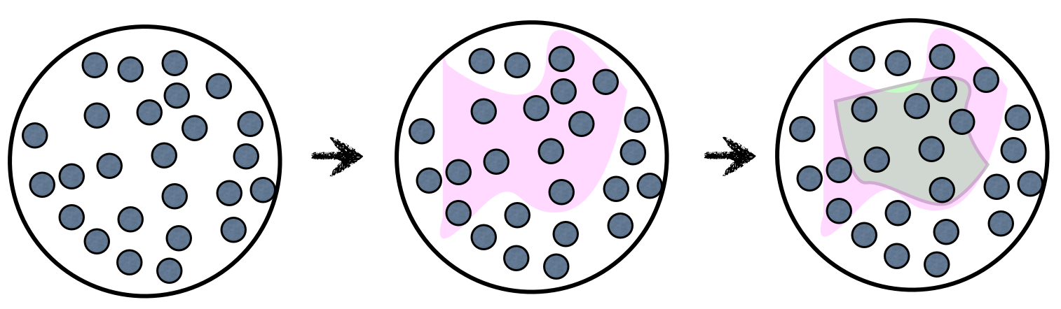
Figure 1: The parent $\mathcal{N}=4$ supersymmetric Yang-Mills theory possesses a plethora of nontrivial flat directions. Some of them are passed down to the FCFT (pink color). Most importantly, a nonzero set of them is not lifted by quantum corrections (green color). On top of these symmetry-breaking vacua, the vacuum energy of the theory is naturally zero.

The extrema of (19) are determined by requiring that the first derivatives of the potential w.r.t. all the fields vanish. A detailed computation [1] reveals that a subclass of the asymmetric classical vacua (13), (14), (16) is robust under quantum corrections. This corresponds to setting $A=B=C=D=0$, and imposing the following extra constraints on the matrix elements

$$\sum_{k=1}^{N_{c}}z_{k}^{2}\log z_{k}=\sum_{k=1}^{N_{c}}\bar{z}_{k}^{2}\log\bar{z}_{k}=0\ .$$ (21)

The vacuum energy of the quantum corrected theory in this Coulomb branch is naturally zero,

$$V_{\rm eff}=0\ ,$$ (22)

or in other words, the dilaton continues being massless at the one-loop level, without finetunings.

It was already pointed out that the FCFT has inherited many of the vacua of its parent $\mathcal{N}=4$ SYM. Although by no means guaranteed, out of them there is a nontrivial subclass which is singled out since they survive quantum corrections, see also Fig. 1.

Before moving on, it is worth pointing out yet another nontrivial feature of the FCFT: many higher loop diagrams that can in principle spoil the flatness of the effective potential, are absent in the planar limit. This is due to the constraints  (14), (16), (21) that force them to vanish on the top of the vacua under consideration. In addition, the non-Hermiticity/fixed chirality of the single-trace interaction acts as a self-protection mechanism in the sense that the “antichiral” vertices that would stem from the nonexistent $\text{tr}(\hbox to0.0pt{\hskip 1.27083pt\leavevmode\hbox{\set@color$\overline{\hbox{}}$}\hss}{\leavevmode\hbox{\set@color$Z$}}\hbox to0.0pt{\hskip 2.0347pt\leavevmode\hbox{\set@color$\overline{\hbox{}}$}\hss}{\leavevmode\hbox{\set@color$X$}}ZX)$ term are now absent. Consequently, another class of dangerous diagrams, such as those presented in Fig.  2(a), cannot be constructed at all. It remains to be understood whether the theory receives no multi-loop contributions at all.

Note, however, that the flatness of the effective potential may be spoiled due to the presence of diagrams like the one of Fig. 2(b), which appears at the $1/N_{c}^{2}$ order. In general, it would not be surprising that some properties of the FCFT do not survive beyond the planar limit (or for finite number of colors), even when the conformal symmetry is linearly realized. This is certainly something that requires separate investigations.

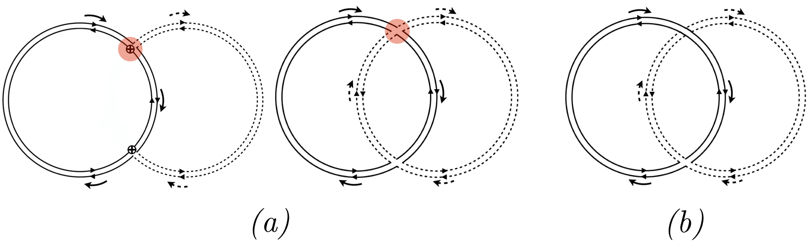
Figure 2: (a) Diagrams at order $\tilde{\xi}^{4}$ that would in principle contribute to the CW potential. A solid (dashed) line stands for the excitations of $X$ ($Z$), and “$\boldsymbol{\otimes}$” for the vev of $Z$. The absent antichiral vertices have been marked with red. (b) A non-planar diagram with one cubic and one quartic vertex that should not be taken into account in the evaluation of the effective potential.

3.3 Quantum vacua: an existence proof

It is instructive to actually present a simple example of a vacuum which satisfies the aforementioned constraints, so the flatness of potential is not ruined. Consider $\langle X\rangle=0$, while the expectation value of the other field $\langle Z\rangle$ is an $N_{c}\times N_{c}$ block-diagonal matrix comprising $N_{c}/4$ diagonal sub-blocks each with dimensions $4\times 4$, i.e.

$$\langle Z\rangle=v\leavevmode\hbox to125.59pt{\vbox to114.21pt{\text{[drawing]}}}\ . {z_{1}} {z_{2}} {z_{3}} {z_{4}} {\ddots} {z_{1}} {z_{2}} {z_{3}} {z_{4}} \left(\vbox{\hrule height=50.01611pt,depth=50.01611pt,width=0.0pt}\right. \left.\vbox{\hrule height=50.01611pt,depth=50.01611pt,width=0.0pt}\right) {z_{1}} {z_{2}} {z_{3}} {z_{4}} {\ddots} {z_{1}} {z_{2}} {z_{3}} {z_{4}} \left(\vbox{\hrule height=50.01611pt,depth=50.01611pt,width=0.0pt}\right. \left.\vbox{\hrule height=50.01611pt,depth=50.01611pt,width=0.0pt}\right)$$ (23)

With this ansatz, the set of the transcendental equations (14), (16), (21) admits the following complex numerical solution

$$z_{1}=-0.587849-0.808971\,i\ ,~{}~{}~{}z_{2}=0.260305+1.45187\,i\ ,$$ (24)

$$z_{3}=1.32754-0.642903\,i\ ,~{}~{}~{}~{}~{}~{}\,\,\,\,\,z_{4}=-1\ .$$

More (complicated) vacua can be constructed in a straightforward manner. For instance, one can seek for solutions to eqs. (14), (16), (21) by considering bigger sub-blocks of the same dimension, or even combinations of sub-blocks of different dimensionalities.

4 Conclusions

In the present talk I touched upon conformal symmetry breaking in the context of the FCFT. As it hopefully became clear, this is a rather special theory for a variety of reasons.

First, the theory can accommodate nontrivial vacua without the burden of finetuning the corresponding coupling(s). This is in one-to-one with the dynamical generation of scales, while the vacuum energy is zero, naturally.

Importantly, in the planar limit, the subclass of the classical asymmetric flat directions $\langle X\rangle=0,~{}\langle Z\rangle\neq 0$ given by (13) and subject to (14), (16) and (21), was shown to not be lifted by quantum effects, at least at the one-loop order. In other words, the FCFT exhibits nonlinear realization of exact quantum conformal symmetry.

Such unique features are the aftermath of: i) the model’s non-Hermiticity that translates into a fixed orientation of the interaction vertices;  ii) the fact that the considerations concern the large-$N_{c}$ limit; iii) the constraints (14), (16) and (21) on the flat directions.

Although the phenomenological relevance of the FCFT per se is not clear, the theory is an ideal playground for studying the dynamics underlying the spontaneous breaking of quantum conformal symmetry. For example, confronting it with the consistency conditions on the CFT data presented in [78], may shed light on general properties shared also by realistic effective field theories (see also footnote 2) exhibiting nonlinearly realized exact conformal invariance. This can be a step towards understanding to what extent CFTs are in the heart of the solutions to the Standard Model finetuning issues.

- [1] G. K. Karananas, V. Kazakov and M. Shaposhnikov, Spontaneous Conformal Symmetry Breaking in Fishnet CFT, 1908.04302.
- [2] O. Gurdogan and V. Kazakov, New Integrable 4D Quantum Field Theories from Strongly Deformed Planar 4 Supersymmetric Yang-Mills Theory, Phys. Rev. Lett. 117 (2016) 201602 [1512.06704].
- [3] N. Gromov, V. Kazakov, G. Korchemsky, S. Negro and G. Sizov, Integrability of Conformal Fishnet Theory, JHEP 01 (2018) 095 [1706.04167].
- [4] D. Chicherin, V. Kazakov, F. Loebbert, D. Müller and D.-l. Zhong, Yangian Symmetry for Fishnet Feynman Graphs, Phys. Rev. D96 (2017) 121901 [1708.00007].
- [5] D. Grabner, N. Gromov, V. Kazakov and G. Korchemsky, Strongly -Deformed Supersymmetric Yang-Mills Theory as an Integrable Conformal Field Theory, Phys. Rev. Lett. 120 (2018) 111601 [1711.04786].
- [6] V. Kazakov and E. Olivucci, Biscalar Integrable Conformal Field Theories in Any Dimension, Phys. Rev. Lett. 121 (2018) 131601 [1801.09844].
- [7] N. Gromov, V. Kazakov and G. Korchemsky, Exact Correlation Functions in Conformal Fishnet Theory, JHEP 08 (2019) 123 [1808.02688].
- [8] B. Basso and L. J. Dixon, Gluing Ladder Feynman Diagrams into Fishnets, Phys. Rev. Lett. 119 (2017) 071601 [1705.03545].
- [9] B. Basso and D.-l. Zhong, Continuum limit of fishnet graphs and AdS sigma model, JHEP 01 (2019) 002 [1806.04105].
- [10] S. Derkachov, V. Kazakov and E. Olivucci, Basso-Dixon Correlators in Two-Dimensional Fishnet CFT, JHEP 04 (2019) 032 [1811.10623].
- [11] G. P. Korchemsky, Exact scattering amplitudes in conformal fishnet theory, JHEP 08 (2019) 028 [1812.06997].
- [12] A. C. Ipsen, M. Staudacher and L. Zippelius, The one-loop spectral problem of strongly twisted = 4 Super Yang-Mills theory, JHEP 04 (2019) 044 [1812.08794].
- [13] B. Basso, J. Caetano and T. Fleury, Hexagons and Correlators in the Fishnet Theory, JHEP 11 (2019) 172 [1812.09794].
- [14] V. Kazakov, E. Olivucci and M. Preti, Generalized Fishnets and Exact Four-Point Correlators in Chiral CFT4, JHEP 06 (2019) 078 [1901.00011].
- [15] R. de Mello Koch, W. LiMing, H. J. R. Van Zyl and J. P. Rodrigues, Chaos in the Fishnet, Phys. Lett. B793 (2019) 169 [1902.06409].
- [16] N. Gromov and A. Sever, Derivation of the Holographic Dual of a Planar Conformal Field Theory in 4D, Phys. Rev. Lett. 123 (2019) 081602 [1903.10508].
- [17] N. Gromov and A. Sever, Quantum fishchain in AdS5, JHEP 10 (2019) 085 [1907.01001].
- [18] S. Dutta Chowdhury, P. Haldar and K. Sen, On the Regge limit of Fishnet correlators, JHEP 10 (2019) 249 [1908.01123].
- [19] N. Gromov and A. Sever, The holographic dual of strongly -deformed = 4 SYM theory: derivation, generalization, integrability and discrete reparametrization symmetry, JHEP 02 (2020) 035 [1908.10379].
- [20] T. Adamo and S. Jaitly, Twistor fishnets, J. Phys. A53 (2020) 055401 [1908.11220].
- [21] B. Basso, G. Ferrando, V. Kazakov and D.-l. Zhong, Thermodynamic Bethe Ansatz for Fishnet CFT, 1911.10213.
- [22] M. Alfimov, N. Gromov and V. Kazakov, SYM Quantum Spectral Curve in BFKL regime, 2020, 2003.03536.
- [23] J. Caetano, Ö. Gürdoğan and V. Kazakov, Chiral limit of = 4 SYM and ABJM and integrable Feynman graphs, JHEP 03 (2018) 077 [1612.05895].
- [24] D. J. Amit and E. Rabinovici, Breaking of Scale Invariance in Theory: Tricriticality and Critical End Points, Nucl. Phys. B257 (1985) 371.
- [25] M. B. Einhorn, G. Goldberg and E. Rabinovici, Quasirenormalizable Models, Nucl. Phys. B256 (1985) 499.
- [26] E. Rabinovici, B. Saering and W. A. Bardeen, Critical Surfaces and Flat Directions in a Finite Theory, Phys. Rev. D36 (1987) 562.
- [27] M. Shaposhnikov and D. Zenhausern, Quantum scale invariance, cosmological constant and hierarchy problem, Phys. Lett. B671 (2009) 162 [0809.3406].
- [28] F. Englert, C. Truffin and R. Gastmans, Conformal Invariance in Quantum Gravity, Nucl. Phys. B117 (1976) 407.
- [29] C. Wetterich, Cosmologies With Variable Newton’s ’Constant’, Nucl. Phys. B302 (1988) 645.
- [30] C. Wetterich, Cosmology and the Fate of Dilatation Symmetry, Nucl. Phys. B302 (1988) 668 [1711.03844].
- [31] C. Wetterich, The Cosmon model for an asymptotically vanishing time dependent cosmological ’constant’, Astron. Astrophys. 301 (1995) 321 [hep-th/9408025].
- [32] W. A. Bardeen, On naturalness in the standard model, in Ontake Summer Institute on Particle Physics Ontake Mountain, Japan, August 27-September 2, 1995.
- [33] K. A. Meissner and H. Nicolai, Conformal Symmetry and the Standard Model, Phys. Lett. B648 (2007) 312 [hep-th/0612165].
- [34] M. Shaposhnikov and D. Zenhausern, Scale invariance, unimodular gravity and dark energy, Phys. Lett. B671 (2009) 187 [0809.3395].
- [35] M. E. Shaposhnikov and F. V. Tkachov, Quantum scale-invariant models as effective field theories, 0905.4857.
- [36] D. Blas, M. Shaposhnikov and D. Zenhausern, Scale-invariant alternatives to general relativity, Phys. Rev. D84 (2011) 044001 [1104.1392].
- [37] J. Garcia-Bellido, J. Rubio, M. Shaposhnikov and D. Zenhausern, Higgs-Dilaton Cosmology: From the Early to the Late Universe, Phys. Rev. D84 (2011) 123504 [1107.2163].
- [38] F. Bezrukov, G. K. Karananas, J. Rubio and M. Shaposhnikov, Higgs-Dilaton Cosmology: an effective field theory approach, Phys. Rev. D87 (2013) 096001 [1212.4148].
- [39] R. Armillis, A. Monin and M. Shaposhnikov, Spontaneously Broken Conformal Symmetry: Dealing with the Trace Anomaly, JHEP 10 (2013) 030 [1302.5619].
- [40] G. Marques Tavares, M. Schmaltz and W. Skiba, Higgs mass naturalness and scale invariance in the UV, Phys. Rev. D89 (2014) 015009 [1308.0025].
- [41] F. Gretsch and A. Monin, Perturbative conformal symmetry and dilaton, Phys. Rev. D92 (2015) 045036 [1308.3863].
- [42] V. V. Khoze, Inflation and Dark Matter in the Higgs Portal of Classically Scale Invariant Standard Model, JHEP 11 (2013) 215 [1308.6338].
- [43] J. Rubio and M. Shaposhnikov, Higgs-Dilaton cosmology: Universality versus criticality, Phys. Rev. D90 (2014) 027307 [1406.5182].
- [44] R. H. Boels and W. Wormsbecher, Spontaneously broken conformal invariance in observables, 1507.08162.
- [45] A. Karam and K. Tamvakis, Dark matter and neutrino masses from a scale-invariant multi-Higgs portal, Phys. Rev. D92 (2015) 075010 [1508.03031].
- [46] G. K. Karananas and M. Shaposhnikov, Scale invariant alternatives to general relativity. II. Dilaton properties, Phys. Rev. D93 (2016) 084052 [1603.01274].
- [47] G. K. Karananas and J. Rubio, On the geometrical interpretation of scale-invariant models of inflation, Phys. Lett. B761 (2016) 223 [1606.08848].
- [48] A. Karam and K. Tamvakis, Dark Matter from a Classically Scale-Invariant , Phys. Rev. D94 (2016) 055004 [1607.01001].
- [49] P. G. Ferreira, C. T. Hill and G. G. Ross, Weyl Current, Scale-Invariant Inflation and Planck Scale Generation, Phys. Rev. D95 (2017) 043507 [1610.09243].
- [50] J. Rubio and C. Wetterich, Emergent scale symmetry: Connecting inflation and dark energy, Phys. Rev. D96 (2017) 063509 [1705.00552].
- [51] S. Casas, M. Pauly and J. Rubio, Higgs-dilaton cosmology: An inflation–dark-energy connection and forecasts for future galaxy surveys, Phys. Rev. D97 (2018) 043520 [1712.04956].
- [52] P. G. Ferreira, C. T. Hill and G. G. Ross, Inertial Spontaneous Symmetry Breaking and Quantum Scale Invariance, Phys. Rev. D98 (2018) 116012 [1801.07676].
- [53] D. Gorbunov and A. Tokareva, Scalaron the healer: removing the strong-coupling in the Higgs- and Higgs-dilaton inflations, Phys. Lett. B788 (2019) 37 [1807.02392].
- [54] S. Casas, G. K. Karananas, M. Pauly and J. Rubio, Scale-invariant alternatives to general relativity. III. The inflation-dark energy connection, Phys. Rev. D99 (2019) 063512 [1811.05984].
- [55] S. Mooij, M. Shaposhnikov and T. Voumard, Hidden and explicit quantum scale invariance, Phys. Rev. D99 (2019) 085013 [1812.07946].
- [56] M. Shaposhnikov and K. Shimada, Asymptotic Scale Invariance and its Consequences, Phys. Rev. D99 (2019) 103528 [1812.08706].
- [57] A. Karam, Phenomenological and Cosmological Implications of Classically Scale-Invariant Standard Model Extensions, Ph.D. thesis, Ioannina U., 2018.
- [58] P. G. Ferreira, C. T. Hill, J. Noller and G. G. Ross, Scale-independent inflation, Phys. Rev. D100 (2019) 123516 [1906.03415].
- [59] D. M. Ghilencea, Weyl R2 inflation with an emergent Planck scale, JHEP 10 (2019) 209 [1906.11572].
- [60] D. M. Ghilencea, Palatini quadratic gravity: spontaneous breaking of gauged scale symmetry and inflation, 2003.08516.
- [61] C. Wetterich, Quantum scale symmetry, 1901.04741.
- [62] C. Wetterich, Fine Tuning Problem and the Renormalization Group, Phys. Lett. 140B (1984) 215.
- [63] M. Shaposhnikov, Is there a new physics between electroweak and Planck scales?, in Astroparticle Physics: Current Issues, 2007 (APCI07), Budapest, Hungary, June 21-23, 2007, 0708.3550.
- [64] G. K. Karananas and M. Shaposhnikov, Gauge coupling unification without leptoquarks, Phys. Lett. B771 (2017) 332 [1703.02964].
- [65] M. Shaposhnikov and A. Shkerin, Conformal symmetry: towards the link between the Fermi and the Planck scales, Phys. Lett. B783 (2018) 253 [1803.08907].
- [66] M. Shaposhnikov and A. Shkerin, Gravity, Scale Invariance and the Hierarchy Problem, JHEP 10 (2018) 024 [1804.06376].
- [67] A. Shkerin, Dilaton-assisted generation of the Fermi scale from the Planck scale, Phys. Rev. D99 (2019) 115018 [1903.11317].
- [68] M. Shaposhnikov, A. Shkerin and S. Zell, Standard Model Meets Gravity: Electroweak Symmetry Breaking and Inflation, 2001.09088.
- [69] J. Fokken, C. Sieg and M. Wilhelm, Non-conformality of -deformed N = 4 SYM theory, J. Phys. A47 (2014) 455401 [1308.4420].
- [70] V. Kazakov, Quantum Spectral Curve of -twisted SYM theory and fishnet CFT, Rev. Math. Phys. 30 (2018) 293 [1802.02160].
- [71] A. B. Zamolodchikov, “Fishing-net” diagrams as a completely integrable system, Phys. Lett. 97B (1980) 63.
- [72] D. Chicherin, S. Derkachov and A. P. Isaev, Conformal group: R-matrix and star-triangle relation, JHEP 04 (2013) 020 [1206.4150].
- [73] C. Sieg and M. Wilhelm, On a CFT limit of planar -deformed SYM theory, Phys. Lett. B756 (2016) 118 [1602.05817].
- [74] S. Fubini, A New Approach to Conformal Invariant Field Theories, Nuovo Cim. A34 (1976) 521.
- [75] F. Coradeschi, P. Lodone, D. Pappadopulo, R. Rattazzi and L. Vitale, A naturally light dilaton, JHEP 11 (2013) 057 [1306.4601].
- [76] S. R. Coleman and E. J. Weinberg, Radiative Corrections as the Origin of Spontaneous Symmetry Breaking, Phys. Rev. D7 (1973) 1888.
- [77] S. R. Coleman, R. Jackiw and H. D. Politzer, Spontaneous Symmetry Breaking in the O(N) Model for Large N*, Phys. Rev. D10 (1974) 2491.
- [78] G. K. Karananas and M. Shaposhnikov, CFT data and spontaneously broken conformal invariance, Phys. Rev. D97 (2018) 045009 [1708.02220].