Thermal dilepton production in collisional hot QCD medium in the presence of chromo-turbulent fields

Abstract

The effects of collisional processes in the hot QCD medium to thermal dilepton production from $q\overline{q}$ annihilation in relativistic heavy-ion collisions have been investigated. The non-equilibrium corrections to the momentum distribution function have been estimated within the framework of ensemble-averaged diffusive Vlasov-Boltzmann equation, encoding the effects of collisional processes and turbulent chromo-fields in the medium. The contributions from the $2\rightarrow 2$ elastic scattering processes have been quantified for the thermal dilepton production rate. It is seen that the collisional corrections enhance the equilibrium dilepton spectra at high $p_{T}$ and suppress at lower $p_{T}$. A comparative study between collisional and anomalous contributions to the dilepton production rates has also been explored. The collisional contributions are seen to be marginal over that due to collisionless anomalous transport.

I Introduction

Heavy-ion collision experiments at Relativistic Heavy Ion Collider (RHIC), and at Large Hadron Collider (LHC), CERN enable the creation of the strongly coupled matter quark-gluon plasma (QGP) expt , which is assumed to have existed in the very early universe a few microseconds after Big-Bang Hatsuda . In these experiments, heavy nuclei are collided at ultra-relativistic energies to produce an expanding hot fireball. The created matter expands in space and time followed by hadronization with the decrease of temperature (with a cross-over from the deconfined quarks and gluons to hadrons for most of the heavy-ion collisions). The evolution of QGP is successfully studied within the framework of causal relativistic hydrodynamics  Heinz ; Muronga:2003ta ; Romatschke:2007mq ; Gale:2013da ; Romatschke:2017ejr . These studies, along with the experimental observations, suggest the existence of strongly coupled QGP with near-perfect fluid nature hirano . The momentum asymmetry of the QCD medium present during the entire medium expansion may induce instabilities to the chromo-field equations. These instabilities in the rapidly expanding medium can lead to the plasma turbulence in the heavy-ion collisions Dupree ; Asakawa:2006tc . These give rise to the anomalous transport in the medium. The impacts of anomalous transport coefficients due to the momentum asymmetry in the medium are well investigated in the electromagnetic plasmas Abe ; Okada and hot QCD plasmas Asakawa:2006tc ; Majumder:2007zh ; Asakawa:2006jn . There have been several studies on the collisional contributions to the transport parameters for the hot QCD medium Mitra:2016zdw ; Kurian:2019fty . The interplay of anomalous and collisional corrections can be studied by analyzing the signals emitted from various phases of fireball expansion.

Thermal dileptons and photons are one of the most efficient probes of QGP  Feinberg76 ; Shyryak78 ; McLerran:1984ay ; Kajantie:1986dh ; Rapp:2014hha . Since they interact electromagnetically, these thermal radiations can reach the detectors without being rescattered. These radiations are emitted throughout the expansion of the fireball with negligible final-state interactions and can carry information about the hotter phases of the matter as well as the initial state of QGP after collision  Alam:1996fd ; Alam:1999sc ; Peitzmann:2001mz . The dilepton invariant mass spectrum has contributions from various processes throughout the evolution of fireball. The high mass range ($M>3$ GeV) has contributions from the hadronic reactions such as photoproduction processes and jet-dilepton conversion arising from initial hadronic scattering. The decays of vector mesons have a considerable contribution in the low mass range $0.6<M<1.1$ GeV. For $M<0.2$ GeV, we encounter the contribution of pion decays from the hadronic phase. While thermal dileptons from QGP are prominent in the intermediate-mass range, $0.2<M<2.5$ GeV with major contribution coming from the $q\bar{q}$ annihilation process Rapp:1999ej ; Alam:1999sc ; Vujanovic:2013jpa .

The anisotropic and viscous effects on dilepton production have been investigated, such as dissipative effects due to shear viscosity Dusling:2008xj ; Bhatt:2011kx ; Bhalerao:2013aha ; Chandra:2015rdz ; Vujanovic:2017psb . The correction due to bulk viscosity on dilepton production was introduced Bhatt:2011kx and studied too Bhalerao:2013aha ; Chandra:2015rdz ; Vujanovic:2019yih . Recently some works have been done to understand the effect of vorticity and magnetic field in the thermal dilepton production  Bhatt:2018xsx ; Das:2019nzv ; Bandyopadhyay:2016fyd ; Ghosh:2018xhh . In Ref. Chandra:2016dwy , the effect of chromo-Weibel instability in the dilepton production rate has been investigated. It will be an interesting task to study the collisional contributions to thermal dilepton production along with the anomalous corrections. The first step towards this analysis is the proper modelling of the near-equilibrium momentum distribution functions for quarks and gluons while incorporating the effects of collisional aspects and anomalous transport in the medium. This sets the motivation for the present analysis.

The static dilepton production rate from $q\bar{q}$ annihilation in the presence of these corrections is obtained from the relativistic kinetic theory. The dilepton rate is calculated by incorporating the QCD medium interaction effects in the cross-section. The total dilepton yield depends on the temperature profile of the expanding QGP. This is obtained from hydrodynamic modelling by providing appropriate initial conditions and realistic equation of state (EoS). It is crucial to note that the role of EoS is important in analyzing the signals from QGP, such as thermal photons Bhatt:2010 and dileptons Bhatt:2011kx . Here, we employ an effective fugacity quasi-particle model (EQPM) Chandra:2011en ; Chandra:2007ca to incorporate the realistic EoS effects in the analysis. In the current analysis, the near-equilibrium distribution functions are obtained as the modification over these distributions induced by anomalous and collisional processes within an effective transport approach closely following Refs. Asakawa:2006jn ; Chandra:2008hi . The distribution functions thus obtained have been employed to study thermal dilepton spectra.

The paper is organized as follows. Section II is devoted to the estimation of non-equilibrium phase-space momentum distribution function while incorporating the effects of collisional processes, and anomalous transport in the QGP medium is described. In Section III, the thermal dilepton production rates are computed in the presence of collisional processes along with the turbulent fields. Section IV deals with dilepton yields for an expanding QGP in heavy-ion collisions. The results and followed discussions are presented in section V, and finally, we conclude the analysis with an outlook in section VI.

Notations and conventions: We are working in units with $k_{B}=1$, $c=1$, $\hbar=1$. The signature of Minkowski metric used is $\eta_{\mu\nu}=\textrm{diag}(+,-,-,-)$. The term $u^{\mu}$ denotes the fluid four-velocity and is normalized to unity $u^{\mu}u_{\mu}=1$. In the fluid rest frame, $u^{\mu}=(1,0,0,0)$. The quantity $\Delta u_{\mu\nu}=\frac{1}{2}(\nabla_{\mu}u_{\nu}+\nabla_{\nu}u_{\mu})-\frac{1}{3}\Delta_{\mu\nu}\nabla_{\gamma}u^{\gamma}$ defines the traceless symmetric velocity gradient, with $\Delta_{\mu\nu}\equiv\eta_{\mu\nu}-u_{\mu}u_{\nu}$ being the projection operator orthogonal to $u^{\mu}$ and $\nabla_{\mu}=\Delta_{\mu\nu}\partial^{\nu}$.

II Modified quark (antiquark) distribution function

Here, a momentum anisotropic hot QCD medium is considered, keeping the fact in mind that momentum anisotropy may sustain in the latter stage of the collisions. The momentum anisotropy may lead to chromo-Weibel instability whose physics is captured in terms of an effective diffusive Vlasov-Boltzmann term depicting the anomalous transport in the hot QCD medium Asakawa:2006tc . It has been argued that the anomalous viscosity dominates over the collisional viscosity in the regime of weak coupling Asakawa:2006jn . The linear transport equation in the presence of turbulent color fields with a collisional term where $2\rightarrow 2$ elastic contributions have been taken into account. The ansatz for the momentum anisotropic/near-equilibrium distribution functions for gluonic and quark/anti-quark degrees of freedom in hot QCD medium is of the form,

$$f_{g/q}({\vec{p}},{\vec{r}})=f_{0~{}g/q}\left[1+(1\pm f_{0~{}g/q})f_{1~{}g/q}({\vec{p}})\right],$$ (1)

where $f_{0}$ and $f_{1}$ denotes the equilibrium and linear order perturbation to the distribution function, respectively. Before obtaining the deviation of momentum distribution function away from equilibrium that encodes the effects of anomalous transport as well as collisional processes, adequate modelling of equilibrium distribution functions for the gluons and quarks has to be considered to incorporate the realistic EoS in the analysis. The EQPM employed in the current analysis interprets the thermal QCD medium EoS with the non-interacting quasigluons and quasiquarks/antiquarks with effective fugacities $z_{g/q}$ and have the following distribution functions Chandra:2011en ; Chandra:2007ca ,

$$f_{0~{}g/q}=\frac{z_{g/q}\exp{(-\beta E_{p})}}{1\mp z_{g/q}\exp{(-\beta E_{p})}},$$ (2)

where $E_{p}=\mid\vec{p}\mid\equiv p$ for gluons and $E_{p}=\sqrt{p^{2}+m^{2}}$ for quarks. The physical significance of the effective fugacity parameter can be understood from the non-trivial energy dispersion relation,

$$\omega_{p}=E_{p}+\delta\omega_{g/q}, \delta\omega_{g/q}=T^{2}\partial_{T}\ln(z_{g/q}),$$ (3)

where $\delta\omega_{g/q}$ denotes the modified part of the dispersion relation. The temperature dependence of effective fugacities can be obtained from the lattice EoS Chandra:2011en . The fugacity parameters are not associated with any conserved current in the medium and retain the same form for quarks and antiquarks Bhadury:2019xdf . The QCD thermodynamics has been studied within the EQPM description, and the results have been compared with that of the lattice data Chandra:2011en . It is observed that the EQPM results are in agreement with the lattice data beyond the transition temperature. In particular, the model accurately describes the trace anomaly of the medium. Further, an effective covariant kinetic theory has been developed within the EQPM to study the near-equilibrium dynamics of the QCD medium Mitra:2018akk . It is important to emphasize that a Virial expansion for the QCD medium has been obtained in terms of quasiparticle number densities to study the QCD interaction. The comparison of the EQPM with other approaches (effective mass model, models based on Polyakov loop, etc.) has been conducted in Ref. Chandra:2011en . The EQPM and the followed effective transport theory approach have been employed to study the transport properties Mitra:2017sjo ; Kurian:2018qwb and momentum anisotropy Kumar:2017bja ; Jamal:2018mog of the QCD medium.

We choose the following ansatz for the linear order perturbation $f_{1~{}g/q}({\vec{p}})$ to the isotropic gluon and quarks distribution functions

$$f_{1~{}g/q}({\vec{p}})=\frac{\bar{\Delta}_{1~{}g/q}({\vec{p}})}{\omega_{p}T^{2}}p^{\mu}p^{\nu}\Delta u_{\mu\nu}.$$ (4)

In the local rest frame of the fluid, we can write $\Delta u_{ij}=-[\frac{1}{2}(\nabla_{i}u_{j}+\nabla_{j}u_{i})-\frac{1}{3}\delta_{ij}\nabla\cdot u]$. Now, considering the boost invariant longitudinal Bjorken’s flow, with $u=\frac{z}{\tau}$ and $\Delta u_{ij}=-\frac{1}{3\tau}\text{diag}(-1,-1,2)$, the expression for $f_{1~{}g/q}({\vec{p}})$ becomes

$$f_{1~{}g/q}({\vec{p}})=-\frac{\bar{\Delta}_{1~{}g/q}({\vec{p}})}{\omega_{p}T^{2}\tau}\left(p_{z}^{2}-\frac{p^{2}}{3}\right),$$ (5)

where $\tau$ is the proper time. In the current analysis, we investigate two dominant sources of the non-equilibrium dynamics of the QGP medium, namely, momentum anisotropy of the QGP medium, and collisional processes in the medium. The strength of the turbulent fields depends on the magnitude of the momentum anisotropy in the medium and gives rise to anomalous transport in the medium. Both these non-equilibrium effects will contribute to shear viscosity as the relaxation rates due to both processes are additive (anomalous and collisional contributions to the viscosity as described in Ref. Asakawa:2006tc ). These non-equilibrium effects are embedded in the analysis through $f_{1~{}g/q}({\vec{p}})$. The momentum anisotropy may induce instabilities in the rapidly expanding medium, which can lead to plasma turbulence, and the turbulent fields give rise to anomalous transport in the medium. The non-equilibrium corrections to the momentum distribution function can be estimated within the framework of ensemble-averaged diffusive Vlasov-Boltzmann equation, encoding the effects of collisional processes and turbulent chromo-fields in the medium. The quantity $\bar{\Delta}_{1~{}g/q}({\vec{p}})$ captures the strength of non-equilibrium part of the distribution function. For the case with only anomalous transport (where collisional aspects are negligible) $\bar{\Delta}_{1~{}g/q}({\vec{p}})$ can be defined as follows Asakawa:2006tc ; Chandra:2016dwy ,

$$\bar{\Delta}_{1~{}g/q}({{\vec{p}}})=2(N_{c}^{2}-1)\dfrac{\omega_{g/q}T}{3g^{2}C_{2}\langle E^{2}+B^{2}\rangle_{g/q}\tau_{m}},$$ (6)

where unknown factors in the denominator is related to the jet quenching parameter $\hat{q}$. Here, $\langle E^{2}\rangle$ and $\langle B^{2}\rangle$ represent the color averaged chromo-electromagnetic fields and $\tau_{m}$ measures the time scale of instability in the medium. The current focus is to incorporate the collisional aspects along with the anomalous contributions to the momentum distribution functions. For the general case, $\bar{\Delta}_{1~{}g/q}({\vec{p}})$ takes the following form,

$$\bar{\Delta}_{1~{}g/q}({\vec{p}})=\frac{{A_{g/q}^{t}}|\vec{p}|}{T}.$$ (7)

Here, the quantity $A_{g/q}^{t}$ has contributions from both anomalous and collisional transports. The effect of collisional processes in the evolution of distribution function can be quantified with the collision kernel in the transport equation. From Eq. (5), the leading order correction to the quark distribution function can be considered as,

$$f_{1~{}q}=-\frac{{A_{q}^{t}}|\vec{p}|}{\omega_{p}(T,\vec{p})T^{3}\tau}\left(p_{z}^{2}-\frac{p^{2}}{3}\right),$$ (8)

where $\omega_{p}^{-1}$ takes the following form in the linear expansion,

$$\omega_{p}^{-1}(T,\vec{p})\approx\left[\frac{1}{|\vec{p}|}-\frac{\delta\omega_{q}}{|\vec{p}|^{2}}\right].$$ (9)

The authors of the Ref. Mitra:2017sjo have realized that the leading order (in temperature gradient of effective fugacity) correction to single particle energy is less than $10\%$ at $T=2.5T_{c}$ and observed considerable agreement in the results of transport coefficients from full numerical coding and from the linear expansion approximation. Note that we are not considering the subscript for quarks while defining the distribution function and dispersion relation as the current focus is on the dilepton production by $q\bar{q}$ annihilation. Combining Eqs. (8) and (9), we obtain the form of $f_{1~{}q}$ as

$$f_{1~{}q}=-\frac{{A_{q}^{t}}}{T^{3}\tau}\left[1-\frac{\delta\omega_{q}}{|\vec{p}|}\right]\left(p_{z}^{2}-\frac{p^{2}}{3}\right).$$ (10)

Similarly, one can estimate the non-equilibrium corrections to the gluon distribution function in terms of ${A_{g}^{t}}$.

The form of ${A_{g/q}^{t}}$

Following the same formalism as in Refs. Chandra:2016dwy ; Asakawa:2006jn , one can estimate the algebraic equation of ${A_{g/q}^{t}}$ by taking the appropriate moment of the transport equation. The ensemble average Vlasov-Boltzmann equation takes the form as follows,

$$v^{\mu}\dfrac{\partial}{\partial x^{\mu}}\bar{f}-\mathcal{F}_{A}\bar{f}+\langle C[f]\rangle=0,$$ (11)

where $\bar{f}$ is the ensemble-averaged thermal distribution of the particles. In our case, $\bar{f}\equiv f_{g/q}$ as defined in the Eq. (1). The diffusive Vlasov term characterizes the contribution from turbulent fields, and the force term takes the form as,

$$\mathcal{F}_{A}\bar{f}= \dfrac{g^{2}C_{f}}{3(N_{c}^{2}-1)\omega_{g,q}}\langle E^{2}+B^{2}\rangle_{g,q}\tau_{m}$$

$$\times\mathcal{L}^{2}f_{0~{}g/q}(1\pm f_{0~{}g/q})p_{i}p_{j}\Delta u_{ij},$$ (12)

with $C_{f}$ is the Casimir invariant of $SU(N_{c})$ gauge theory and the operator $\mathcal{L}^{2}$ can be defined as,

$$\mathcal{L}^{2}=\mid\vec{p}\times\partial_{\vec{p}}\mid^{2}-\mid\vec{p}\times\partial_{\vec{p}}\mid^{2}_{z}.$$ (13)

In the current analysis, $A^{t}$ has contributions from both anomalous and collisional transports. For the anomalous transport, the strength of the turbulent fields are related to the anomalous transport in the medium. In addition, we have switched on the collisional term in the Boltzmann equation which contribute to the collisional aspects of the medium. The collision kernel $\langle C[f]\rangle$ in the transport equation measures the leading order contributions from the collisional processes. The collision integral for the $2\rightarrow 2$ scattering process $\vec{p},\vec{k}\rightarrow\vec{p}^{{}^{\prime}},\vec{k}^{{}^{\prime}}$ is defined as Asakawa:2006jn ; Arnold:2000dr ,

$$C[f]= \dfrac{1}{4E_{p}}\int{\dfrac{d^{3}{\vec{k}}}{(2\pi)^{3}2E_{k}}}\int{\dfrac{d^{3}{\vec{p}}^{{}^{\prime}}}{(2\pi)^{3}2E_{p^{{}^{\prime}}}}}\int{\dfrac{d^{3}{\vec{k}}^{{}^{\prime}}}{(2\pi)^{3}2E_{k^{{}^{\prime}}}}}$$

$$\times|\mathcal{M}|^{2}(2\pi)^{4}\delta^{4}(P+K-P^{{}^{\prime}}-K^{{}^{\prime}})$$

$$\times\Bigg{[}f_{g/q}({\vec{p}})f_{g/q}({\vec{k}})\Big{(}1\pm f_{g/q}({\vec{p}}^{{}^{\prime}})\Big{)}\Big{(}1\pm f_{g/q}({\vec{k}}^{{}^{\prime}})\Big{)}$$

$$-f_{g/q}({\vec{p}^{{}^{\prime}}})f_{g/q}({\vec{k}})\Big{(}1\pm f_{g/q}({\vec{p}})\Big{)}\Big{(}1\pm f_{g/q}({\vec{k}})\Big{)}\Bigg{]},$$ (14)

where $|\mathcal{M}|^{2}$ is the scattering amplitude and $P,K,P^{{}^{\prime}}$ and $K^{{}^{\prime}}$ are the four-momenta of the particles before and after scattering. The linearized transport equation is a linear integral equation, and one can employ variational method by minimizing the linearized Vlasov-Boltzmann equation to determine $\bar{\Delta}_{1~{}g/q}({\vec{p}})$. Following this standard method as in Refs. Chandra:2016dwy ; Asakawa:2006jn leads to the following matrix equation for the column vector ${A^{t}=\{{A_{g}^{t}},{A_{q}^{t}}\}}$,

$$(\tilde{a}_{A}+\tilde{a}_{C}){A^{t}}=\tilde{r}.$$ (15)

The column vector $\tilde{r}$ takes the form,

$$\tilde{r}=\left\{\frac{32\left(N_{c}^{2}-1\right)I_{5}^{g}}{3\pi^{2}},\frac{32N_{c}N_{f}I_{5}^{q}}{3\pi^{2}}\right\},$$ (16)

where $N_{f}$ is the number of flavors, and the function $I_{n}$ takes the form,

$$I_{n}^{q}=-\rm{PolyLog}[n,-z_{q}], I_{n}^{g}=\rm{PolyLog}[n,z_{g}],$$ (17)

for quarks and gluons. The matrices $\tilde{a}_{A}$ and $\tilde{a}_{C}$ denote the anomalous transport and collisional (elastic scattering processes) contribution of the transport equation. The matrix $\tilde{a}_{A}$ takes the following form,

$$\tilde{a}_{A}=\left(\begin{array}[]{cc}\frac{32N_{c}I_{4}^{g}Q_{g}}{5\pi^{2}T^{3}}&0\\ 0&\frac{32N_{f}I_{4}^{q}Q_{q}}{5\pi^{2}T^{3}}\\ \end{array}\right),$$ (20)

where $Q_{g/q}$ is defined as,

$$Q_{g/q}=\frac{g^{2}\langle E^{2}+B^{2}\rangle_{g,q}}{2}\tau_{m}.$$ (21)

The matrix $\tilde{a}_{C}$ can be described as follows,

$$\tilde{a}_{C}=C_{c}\left(\begin{array}[]{cc}\frac{7N_{c}\left(2N_{c}+N_{f}\right)I_{2}^{g}}{24\pi^{2}z_{g}}+\frac{N_{c}\left(N_{c}^{2}-1\right)N_{f}\left(I_{4}^{g}+I_{4}^{q}\right)z_{g}}{2\pi^{3}\left(z_{g}+z_{q}\right)}&-\frac{N_{c}\left(N_{c}^{2}-1\right)N_{f}\left(I_{4}^{g}+I_{4}^{q}\right)z_{g}}{2\pi^{3}\left(z_{g}+z_{q}\right)}\\ -\frac{N_{c}\left(N_{c}^{2}-1\right)N_{f}\left(I_{4}^{g}+I_{4}^{q}\right)z_{g}}{2\pi^{3}\left(z_{g}+z_{q}\right)}&\frac{7N_{f}\left(2N_{c}+N_{f}\right)I_{2}^{q}}{24\pi^{2}z_{q}}+\frac{N_{c}\left(N_{c}^{2}-1\right)N_{f}\left(I_{4}^{g}+I_{4}^{q}\right)z_{g}}{2\pi^{3}\left(z_{g}+z_{q}\right)}\\ \end{array}\right).$$ (24)

The EQPM is based on the charge renormalization in medium Chandra:2011en , and one can define an effective coupling $\alpha_{eff}$ by investigating the Debye screening mass of the QCD medium Mitra:2017sjo . Note that in the leading-log order, we have $C_{c}\approx 2\pi^{2}(N_{c}^{2}-1)\alpha^{2}_{eff}\log(\alpha_{eff}^{-1})$, where $\alpha_{eff}$ takes the form,

$$\alpha_{eff}=\alpha_{s}(T)\Bigg{(}\dfrac{\frac{2N_{c}}{\pi^{2}}I_{2}^{g}+\frac{2N_{f}}{\pi^{2}}I^{q}_{2}}{\frac{N_{c}}{3}+\frac{N_{f}}{6}}\Bigg{)}.$$ (25)

The 2-loop expression for QCD running coupling constant $\alpha_{s}(T)$ at finite temperature can be defined as Srivastava:2015via ; Haque:2012my ; Laine:2005ai ,

$$\alpha_{s}(T)=\dfrac{6\pi}{(33-2N_{f})\ln{\frac{T}{\Lambda_{T}}}}\Bigg{(}1-\dfrac{3(153-19N_{f})}{(33-2N_{f})^{2}}\dfrac{\ln(2\ln{\frac{T}{\Lambda_{T}}})}{\ln{\frac{T}{\Lambda_{T}}}}\Bigg{)},$$ (26)

with QCD scale fixing parameter can be defined from the $\overline{MS}$ scheme such that $\Lambda_{T}=\frac{\exp(\gamma_{E}+1/22)}{4\pi}\Lambda_{MS}$, where $\gamma_{E}=0.5772156$ and the renormalization scale $\Lambda_{MS}=1.14~{}T_{c}$ Chandra:2007ca . The algebraic forms of ${A_{g}^{t}}$ and ${A_{q}^{t}}$ can be obtained by solving Eq. (15) using Eqs. (16), (20) and  (24) and have the following forms,

$${{A_{g}^{t}}}=\frac{1280\pi\left(N_{c}^{2}-1\right)\Big{(}N_{c}^{2}N_{f}I^{q}_{5}~{}\phi_{0}+I_{5}^{g}~{}\phi_{1}\Big{)}}{N_{c}\Big{(}-N_{c}(N_{c}^{2}-1)^{2}N_{f}\phi^{2}_{0}+\phi_{1}\phi_{2}\Big{)}},$$ (27)

and

$${{A_{q}^{t}}}=\frac{1280\pi\Big{(}(N_{c}^{2}-1)^{2}I^{g}_{5}~{}\phi_{0}+N_{c}I_{5}^{q}~{}\phi_{2}\Big{)}}{-N_{c}(N_{c}^{2}-1)^{2}N_{f}\phi^{2}_{0}+\phi_{1}\phi_{2}}.$$ (28)

The quantities $\phi_{0}$, $\phi_{1}$ and $\phi_{2}$ are defined as follows,

$$\phi_{0} = 60C_{c}\Big{(}I_{4}^{g}+I_{4}^{q}\Big{)}\frac{z_{g}}{z_{g}+z_{q}},$$

$$\phi_{1} = N_{c}(N_{c}^{2}-1)\phi_{0}+\frac{35\pi C_{c}I_{2}^{q}(2N_{c}+N_{f})}{z_{q}}+\frac{768\pi Q_{q}I_{4}^{q}}{T^{3}},$$

$$\phi_{2} = (N_{c}^{2}-1)N_{f}\phi_{0}+\frac{35\pi C_{c}I_{2}^{g}(2N_{c}+N_{f})}{z_{g}}+\frac{768\pi Q_{g}I_{4}^{g}}{T^{3}}.$$

It is important to emphasize that the expressions of ${A_{g}^{t}}$ and ${A_{q}^{t}}$ reduce to the results of Ref. Asakawa:2006jn ; Chandra:2008hi in the limit $z_{g,q}\rightarrow 1$ and in the absence of collisions, $\tilde{a}_{C}=0$.

Next, by employing these non-equilibrium distribution functions, we study the thermal dilepton production from hot QCD medium.

III Thermal dilepton production rate

Thermal dileptons produced in the QGP medium has major contributions from the $q\bar{q}$ annihilation process, $q\bar{q}\rightarrow\gamma^{*}\rightarrow l^{+}l^{-}$. The rate of dilepton production for this process within the EQPM model in terms of quark distribution function can be defined as,

$$\frac{dN}{d^{4}xd^{4}p} = \int\frac{d^{3}\vec{p}_{1}}{(2\pi)^{3}}\frac{d^{3}\vec{p}_{2}}{(2\pi)^{3}}\,\frac{M_{eff}^{2}g_{d}^{2}\sigma(M_{eff}^{2})}{2\omega_{1}\omega_{2}}$$ (29)

$$\times f(\vec{p}_{1})f(\vec{p}_{2})\delta^{4}(\tilde{p}-\tilde{p}_{1}-\tilde{p}_{2}).$$

Note that the subscript $q$ for the distribution function is dropped from this section as the focus is only on the $q\bar{q}$ annihilation process, $i.e.$, $f_{q}(\vec{p})\equiv f(\vec{p})$ and is described in Eq. (1). Here, the quantity $M_{eff}$ is the medium modified effective mass of the virtual photon in the interacting QCD medium with

$$M_{eff}^{2} =(\omega_{1}+\omega_{2})^{2}-(\vec{p}_{1}+\vec{p}_{2})^{2}$$ (30)

$$\approx M^{2}\left(1+\frac{4\delta\omega_{q}(E_{1}+E_{2})}{M^{2}}\right),$$

where $M^{2}$ represents its invariant mass in the limit of $z_{q/g}=1$. The quantity $\tilde{p}_{1,2}=(\omega_{1,2},\,\vec{p}_{1,2})$ is the 4-momenta of the quark and antiquark respectively and $\tilde{p}=(\omega_{0}=\omega_{1}+\omega_{2},\,\vec{p}=\vec{p}_{1}+\vec{p}_{2})$ is the 4-momentum of the dilepton pair. If the quark masses are neglected, we can write $\omega_{1,2}=\sqrt{{\vec{p}_{1,2}}^{2}+m^{2}}\approx|\vec{p}_{1,2}|$. The term $\sigma(M_{eff}^{2})$ is the thermal dilepton production cross section and $g_{d}$ is the degeneracy factor. The relative velocity of the quark-antiquark pair is given by $v_{rel}=\sqrt{\frac{M_{eff}^{2}(M_{eff}^{2}-4m^{2})}{4\omega_{1}^{2}\omega_{2}^{2}}}\simeq\frac{M_{eff}^{2}}{2\omega_{1}\omega_{2}}$. With $N_{f}=2$ and $N_{c}=3$, we have $M_{eff}^{2}g_{d}^{2}\sigma(M_{eff}^{2})=\frac{80\pi}{9}\alpha^{2}$. We are interested in the regime in which invariant masses are larger than the temperature, $M>>T>>m$. Hence we can approximate the Fermi-Dirac distribution by that of the classical Maxwell-Boltzmann distribution (high temperature limit) i.e., $f_{0}(\vec{p})\backsimeq z_{q}e^{-\omega/T}$. Under this approximation, the quark (antiquark) distribution function, described by Eq. (1) and Eq. (10), in the covariant form, becomes:

$$f(\vec{p})\backsimeq z_{q}e^{-\omega/T}\left[1+{\chi^{t}(\vec{p},T)}\tilde{p}^{\mu}\tilde{p}^{\nu}\Delta u_{\mu\nu}\right];$$ (31)

where quasiparticle four-momenta ($\tilde{p}^{\mu}$) are related to the bare momenta ($p^{\mu}$) as $\tilde{p}^{\mu}=p^{\mu}+\delta\omega_{g/q}\,u^{\mu}$ and the quantity ${\chi^{t}(\vec{p},T)}$ represents,

$${\chi^{t}(\vec{p},T)}=\frac{{A_{q}^{t}}}{T^{3}}\left[1-\frac{\delta\omega_{q}}{|\vec{p}|}\right].$$ (32)

Keeping the terms only upto quadratic order in momenta, the dilepton production rate takes the form as follows,

$$\frac{dN}{d^{4}xd^{4}p} = \int\frac{d^{3}\vec{p}_{1}}{(2\pi)^{3}}\frac{d^{3}\vec{p}_{2}}{(2\pi)^{3}}\frac{M_{eff}^{2}g_{d}^{2}\sigma(M_{eff}^{2})}{2\omega_{1}\omega_{2}}$$ (33)

$$\times\left[1+2\,{\chi^{t}(\vec{p},T)}\,\tilde{p}_{1}^{\mu}\tilde{p}_{1}^{\nu}\Delta u_{\mu\nu}\right]$$

$$\times f_{0}(\vec{p}_{1})f_{0}(\vec{p}_{2})\,\delta^{4}(\tilde{p}-\tilde{p}_{1}-\tilde{p}_{2})$$

$$= \frac{dN_{0}}{d^{4}xd^{4}p}+\frac{dN_{\chi}}{d^{4}xd^{4}p};$$

where the equilibrium contribution to dilepton production takes the form

$$\frac{dN_{0}}{d^{4}xd^{4}p} = \int\frac{d^{3}\vec{p}_{1}}{(2\pi)^{6}}\,\frac{M_{eff}^{2}g_{d}^{2}\sigma(M_{eff}^{2})}{2\omega_{1}\omega_{2}}z_{q}^{2}e^{-(\omega_{1}+\omega_{2})/T}$$ (34)

$$\times\delta(\omega_{0}-\omega_{1}-\omega_{2})$$

$$= \frac{z_{q}^{2}}{2}\frac{M_{eff}^{2}g_{d}^{2}\sigma(M_{eff}^{2})}{(2\pi)^{5}}e^{-\omega_{0}/T}.$$

Using Eq. (9), (32) in (33), we write the non-equilibrium contribution to the dilepton production rate as,

$$\frac{dN_{\chi}}{d^{4}xd^{4}p} = 2\int\frac{d^{3}\vec{p}_{1}}{(2\pi)^{6}}\,\frac{M_{eff}^{2}g_{d}^{2}\sigma(M_{eff}^{2})}{2\omega_{1}\omega_{2}}z_{q}^{2}e^{-(\omega_{1}+\omega_{2})/T}$$ (35)

$$\times\frac{A_{q}^{t}}{T^{3}}\left[1-\frac{\delta\omega_{q}}{|\vec{p}_{1}|}\right]\,\tilde{p}_{1}^{\mu}\tilde{p}_{1}^{\nu}\Delta u_{\mu\nu}$$

$$\times\delta(\omega_{0}-\omega_{1}-\omega_{2})$$

$$= I^{\mu\nu}(p)\Delta u_{\mu\nu};$$

where,

$$I^{\mu\nu}(p) = 2\int\frac{d^{3}\vec{p}_{1}}{(2\pi)^{6}}\,\frac{M_{eff}^{2}g_{d}^{2}\sigma(M_{eff}^{2})}{2\omega_{1}\omega_{2}}z_{q}^{2}e^{-(\omega_{1}+\omega_{2})/T}$$ (36)

$$\times\frac{A_{q}^{t}}{T^{3}}\left[1-\frac{\delta\omega_{q}}{|\vec{p}_{1}|}\right]\,\tilde{p}_{1}^{\mu}\tilde{p}_{1}^{\nu}\delta(\omega_{0}-\omega_{1}-\omega_{2}).$$

The general form of the second rank tensor can be constructed using the metric $\eta^{\mu\nu}$, $u^{\mu}$ and $\tilde{p}^{\mu}$ as,

$$I^{\mu\nu}(p)=a_{0}\eta^{\mu\nu}+a_{1}u^{\mu}u^{\nu}+a_{2}\tilde{p}^{\mu}\tilde{p}^{\nu}+a_{3}(u^{\mu}\tilde{p}^{\nu}+u^{\nu}\tilde{p}^{\mu}).$$

Since $u^{\mu}\Delta u_{\mu\nu}=0$ and $\eta^{\mu\nu}\Delta u_{\mu\nu}=0$, only the coefficient $a_{2}$ survives when Eq. (III) is contracted with $\Delta u_{\mu\nu}$. Moreover, we construct a projection operator $P_{\mu\nu}$ such that $a_{2}=P_{\mu\nu}I^{\mu\nu}$. The form of $P_{\mu\nu}$ can be obtained as

$$P_{\mu\nu} = \frac{1}{2|\vec{p}|^{4}}\Big{[}|\vec{p}|^{2}\eta_{\mu\nu}+(2\omega_{0}^{2}+M_{eff}^{2})u_{\mu}u_{\nu}+3\tilde{p}_{\mu}\tilde{p}_{\nu}$$ (38)

$$-6\omega_{0}u_{\mu}\tilde{p}_{\nu}\Big{]}.$$

Incorporating these steps, the non-equilibrium contribution to dilepton rate takes the form as follows,

$$\frac{dN_{\chi}}{d^{4}xd^{4}p}=a_{2}\tilde{p}^{\mu}\tilde{p}^{\nu}\Delta u_{\mu\nu}=\left\{P_{\alpha\beta}I^{\alpha\beta}\right\}\tilde{p}^{\mu}\tilde{p}^{\nu}\Delta u_{\mu\nu}.$$

Employing Eq. (36) and Eq. (38) we have,

$$P_{\alpha\beta}I^{\alpha\beta} = \frac{A_{q}^{t}}{|\vec{p}|^{4}T^{3}}\int\frac{d^{3}\vec{p}_{1}}{(2\pi)^{6}}\,\frac{M_{eff}^{2}g_{d}^{2}\sigma(M_{eff}^{2})}{2\omega_{1}\omega_{2}}z_{q}^{2}e^{-(\omega_{1}+\omega_{2})/T}$$ (40)

$$\times\left[(2\omega_{0}^{2}+M_{eff}^{2})\omega_{1}^{2}+3(\tilde{p}\cdot\tilde{p}_{1})^{2}-6\omega_{0}\omega_{1}(\tilde{p}\cdot\tilde{p}_{1})\right]$$

$$\times\left[1-\frac{\delta\omega_{q}}{|\vec{p}_{1}|}\right]\delta(\omega_{0}-\omega_{1}-\omega_{2})$$

$$= \frac{A_{q}^{t}}{T^{3}}\frac{1}{2|\vec{p}|^{5}}[\mathscr{M}+\mathscr{N}],$$

where $\mathscr{M}$ and $\mathscr{N}$ can be defined as,

$$\mathscr{M} = \int dp_{1}\frac{M_{eff}^{2}g_{d}^{2}\sigma(M_{eff}^{2})}{(2\pi)^{5}}z_{q}^{2}\,e^{-\omega_{0}/T}$$

$$\times\left[(3\omega_{0}^{2}-|\vec{p}|^{2})|\vec{p}_{1}|^{2}-3\omega_{0}M_{eff}^{2}|\vec{p}_{1}|+\frac{3}{4}M_{eff}^{4}\right]$$

$$= \frac{dN_{0}}{d^{4}xd^{4}p}\frac{4}{3}|\vec{p}|^{5},$$

and

$$\mathscr{N} = -\delta\omega_{q}\int dp_{1}\frac{M_{eff}^{2}g_{d}^{2}\sigma(M_{eff}^{2})}{(2\pi)^{5}}z_{q}^{2}\,e^{-\omega_{0}/T}$$

$$\times\left[(3\omega_{0}^{2}-|\vec{p}|^{2})|\vec{p}_{1}|-3\omega_{0}M_{eff}^{2}+\frac{3}{4}\frac{M_{eff}^{4}}{|\vec{p}_{1}|}\right]$$

$$= -\frac{dN_{0}}{d^{4}xd^{4}p}2\delta\omega_{q}\Bigg{[}(2\omega_{0}^{2}-5M_{eff}^{2})\frac{\omega_{0}|\vec{p}|}{2}$$

$$+\frac{3}{4}M_{eff}^{4}\ln\left(\frac{\omega_{0}+|\vec{p}|}{\omega_{0}-|\vec{p}|}\right)\Bigg{]}$$

respectively. Thus, we obtain the non-equilibrium contribution to the dilepton rate as,

$$\frac{dN_{\chi}}{d^{4}xd^{4}p} = \frac{dN_{0}}{d^{4}xd^{4}p}\frac{A_{q}^{t}}{T^{3}}\Bigg{\{}\frac{\delta\omega_{q}}{|\vec{p}|^{5}}\Big{[}(5M_{eff}^{2}-2\omega_{0}^{2})\frac{\omega_{0}|\vec{p}|}{2}$$

$$-\frac{3}{4}M_{eff}^{4}\ln\left(\frac{\omega_{0}+|\vec{p}|}{\omega_{0}-|\vec{p}|}\right)\Big{]}+\frac{2}{3}\Bigg{\}}\tilde{p}^{\mu}\tilde{p}^{\nu}\Delta u_{\mu\nu}.$$

The above calculations are done in the local rest frame of the medium. In a general frame with $4-$velocity $u^{\mu}$ these results become

$$\frac{dN_{0}}{d^{4}xd^{4}p} = \frac{z_{q}^{2}}{2}\frac{M_{eff}^{2}g_{d}^{2}\sigma(M_{eff}^{2})}{(2\pi)^{5}}e^{-u\cdot\tilde{p}/T},$$ (42)

$$\frac{dN_{\chi}}{d^{4}xd^{4}p} = \frac{dN_{0}}{d^{4}xd^{4}p}\tilde{p}^{\mu}\tilde{p}^{\nu}\Delta u_{\mu\nu}[\mathscr{P}+\mathscr{R}],$$ (43)

with

$$\mathscr{P}= \frac{2A_{q}^{t}}{3T^{3}},$$

$$\mathscr{R}= \frac{A_{q}^{t}}{T^{3}}\frac{\delta\omega_{q}}{[(u\cdot\tilde{p})^{2}-M_{eff}^{2}]^{2}}\Bigg{\{}\frac{(u\cdot\tilde{p})}{2}[5M_{eff}^{2}-2(u\cdot\tilde{p})^{2}]$$

$$-\frac{3}{4}\frac{M_{eff}^{4}}{\sqrt{(u\cdot\tilde{p})^{2}-M_{eff}^{2}}}\ln\left(\frac{u\cdot\tilde{p}+\sqrt{(u\cdot\tilde{p})^{2}-M_{eff}^{2}}}{u\cdot\tilde{p}-\sqrt{(u\cdot\tilde{p})^{2}-M_{eff}^{2}}}\right)\Bigg{\}}.$$

Next, we proceed to calculate the dilepton production rate in the presence of anomalous correction by switching off the collisional effects in the medium. To study the impact of anomalous transport separately, we consider the case of $\tilde{a}_{C}=0$ and obtain $A^{a}$ following the same formalism as described in section II. In the collision-less limit ( $i.e.$, $A^{t}=A^{a}$), the linear perturbation of the distribution function can be defined as,

$$f_{1}=\frac{{A_{q}^{a}}}{T^{3}}\tilde{p}^{\mu}\tilde{p}^{\nu}\Delta u_{\mu\nu},$$ (44)

where,

$${A_{q}^{a}}=\frac{20}{9}\frac{C_{f}N_{c}T^{3}}{(N_{c}^{2}-1)\hat{q}}\frac{I_{5}^{q}}{I_{4}^{q}},$$ (45)

with $C_{f}=\frac{N_{c}^{2}-1}{2N_{c}}$ for quarks and $\hat{q}$ as the jet quenching factor. In Ref. Majumder:2007zh , the authors have realized that the parameter $\hat{q}$ is proportional to the mean momentum square per unit length on the particle imparted by turbulent color fields. The strength of the turbulent fields, $\langle E^{2}+B^{2}\rangle_{k}$, can be related to the jet quenching parameter as,

$$\hat{q}=\dfrac{2g^{2}C_{g/f}}{3(N_{c}^{2}-1)}\langle E^{2}+B^{2}\rangle\tau_{m}.$$ (46)

Following a similar procedure, we can obtain the non-equilibrium contribution (without collisional effects) to the dilepton production rate as,

$$\frac{dN_{\chi}}{d^{4}xd^{4}p}=\frac{dN_{0}}{d^{4}xd^{4}p}\frac{2{A_{q}^{a}}}{3T^{3}}\tilde{p}^{\mu}\tilde{p}^{\nu}\Delta u_{\mu\nu}.$$ (47)

The total dilepton production rate for this case is obtained by adding the expressions Eq. (42) and Eq. (47),

$$\frac{dN}{d^{4}xd^{4}p}=\frac{dN_{0}}{d^{4}xd^{4}p}\left[1+\frac{2{A_{q}^{a}}}{3T^{3}}\tilde{p}^{\mu}\tilde{p}^{\nu}\Delta u_{\mu\nu}\right].$$ (48)

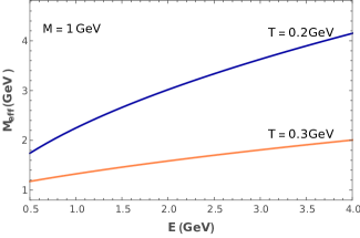
Figure 1: $M_{eff}$ dependence on energy for various temperatures.

Now, we write the thermal dilepton yields obtained in the limit $M_{eff}\rightarrow M$, i.e., when the modifications on $M$ due to the medium effects are neglected. We note that in this limit, the expression for $M_{eff}^{2}$ reduces to $M^{2}=(E_{1}+E_{2})^{2}-(\vec{p}_{1}+\vec{p}_{2})^{2}$, the invariant mass of virtual photon. Here, $p_{1,2}=(E_{1,2},\vec{p}_{1,2})$ represents the $4-$momenta of the quark and antiquark. Also, the $4-$momentum of dilepton reduces to $p^{\mu}=(p_{0}=E_{1}+E_{2},\vec{p}=\vec{p}_{1}+\vec{p}_{2})$. Now, within this limit, the rate of dilepton production for $q\bar{q}$ annihilation process given by Eq. (29) takes the form rvogt ,

$$\frac{dN}{d^{4}xd^{4}p} = \int\frac{d^{3}\vec{p}_{1}}{(2\pi)^{3}}\frac{d^{3}\vec{p}_{2}}{(2\pi)^{3}}\,\frac{M^{2}g_{d}^{2}\sigma(M^{2})}{2E_{1}E_{2}}$$ (49)

$$\times f(\vec{p}_{1})f(\vec{p}_{2})\delta^{4}(p-p_{1}-p_{2}).$$

The cross-section for this process in Born approximation is well known and with $N_{f}=2$, $N_{c}=3$ we have $M^{2}g_{d}^{2}\sigma(M^{2})=\frac{80\pi}{9}\alpha^{2}$  Alam:1996fd ; Domokos:1980ba .

Within this limit, the equilibrium contribution to thermal dilepton rate has the form Chandra:2015rdz

$$\frac{dN_{0}}{d^{4}xd^{4}p} = \int\frac{d^{3}\vec{p}_{1}}{(2\pi)^{6}}\,z_{q}^{2}e^{-(E_{1}+E_{2})/T}\frac{M^{2}g_{d}^{2}\sigma(M^{2})}{2E_{1}E_{2}}$$ (50)

$$\times\delta(p_{0}-E_{1}-E_{2})$$

$$= z_{q}^{2}\times\frac{1}{2}\frac{M^{2}g_{d}^{2}\sigma(M^{2})}{(2\pi)^{5}}e^{-(u\cdot p)/T}.$$

The non-equilibrium contributions to the dilepton production rate, with and without the collisional terms are obtained by taking the limit $M_{eff}\rightarrow M$ in the Eqs. (43) and (48) respectively.

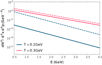
Figure 2: Equilibrium dilepton production rate plotted against $E$. The dashed lines represent the rates in the limit $M_{eff}\rightarrow M$.

Now, we analyze the strength of the medium interaction effects on thermal dilepton rates. As a first step to this analysis, we examine the temperature dependence of $M_{eff}$. Fig. 1 shows $M_{eff}$ plotted for various energies with $M=1$ GeV. It is evident that the impact of medium effects is more dominant at low temperatures. Also, we note that irrespective of the value of $M$, at high temperature, $M_{eff}$ approaches $M$, which is indicative of the fact that the interaction term vanishes with the increase of temperature. In Fig. 2, we analyze the strength of these interaction terms on thermal dilepton rate by plotting the equilibrium dilepton production rate obtained within the quasi-particle prescription (Eq. (50), denoted by solid lines) along with the one calculated in the limit $M_{eff}\rightarrow M$ (Eq. (42), represented by dashed lines). It is observed that the presence of medium interaction effects suppresses the dilepton rates at all energies. This suppression is notably high at low temperatures, which indicates the presence of strong medium effects at low temperatures. Here, we note that the medium interaction effects have a significant impact on the dilepton rates and hence these effects has to be incorporated in the following analysis.

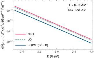
Figure 3: Comparison of dilepton rate calculated within EQPM along with the strict NLO results for dilepton production. LO and NLO rates are taken from Ref. Laine:2013vma .

Note that, in the present work, we focus on the $q\bar{q}$ annihilation process of dilepton production in the Born approximation. However, there are other dilepton rate calculations in the presence of higher-order corrections Song:2018dvf ; Laine:2013vma ; Laine:2015iia ; Aurenche:2002wq . In Fig. 3, we show a comparison of production rate of $\mu^{+}\mu^{-}$ pairs calculated within the EQPM (for $\delta f=0$) with the strict next-to-leading order (NLO) results of Ref Laine:2013vma . The leading order (LO) rate is also plotted for comparison. The rates are plotted as a function of the energy of the dilepton pair ($E$) for a fixed temperature, $T=0.3$ GeV, and invariant mass, $M=1.5$ GeV. For this analysis, we evaluate the dilepton rate given by Eq. (49) without considering the Maxwell-Boltzmann approximation. Also, we take $N_{c}=N_{f}=3$ for this comparison. From fig. 3, it can be seen that the presence of fugacity parameter suppresses the $\mu^{+}\mu^{-}$ rate when compared to LO results for all dilepton energies. This is in line with the result obtained in Ref. Chandra:2016dwy . It is also observed that while comparison with NLO results, the EQPM rate suffers more decrement compared to the previous case.

IV Thermal dilepton yield from expanding QGP

Dilepton yield from QGP in heavy-ion collisions can be studied by obtaining the temperature profile of the system. This can be done by modelling the expansion of QGP using relativistic hydrodynamics. We employ the longitudinal boost invariant flow model of Bjorken to study the expansion of the system. In this model, the coordinates are parametrized as $t=\tau\cosh\eta_{s}$ and $z=\tau\sinh\eta_{s}$, where, $\tau=\sqrt{t^{2}-z^{2}}$, is the proper time and $\eta_{s}=\frac{1}{2}\ln\left[\frac{t+z}{t-z}\right]$ is the space-time rapidity of the system and the fluid $4-$velocity is expressed as $u^{\mu}=(\cosh\eta_{s},0,0,\sinh\eta_{s})$ Bjorken . Now, four dimensional volume element is given by $d^{4}x=\pi R_{A}^{2}d\eta_{s}\tau d\tau$, where $R_{A}=1.2A_{a}^{1/3}$ is the radius of the nucleus used for collision (for $Au$, $A_{a}=197$). The $4-$momentum of the dilepton can be parametrized as $\tilde{p}^{\alpha}=(M_{T}\cosh y,p_{T}\cos\phi_{p},p_{T}\sin\phi_{p},M_{T}\sinh y)$, where $M_{T}^{2}=p_{T}^{2}+M_{eff}^{2}$. Now, the factors appearing in the rate expression under Bjorken expansion can be calculated as

$$u\cdot\tilde{p}= M_{T}\cosh(y-\eta_{s}),$$ (51)

$${\tilde{p}^{\mu}\tilde{p}^{\nu}\Delta u_{\mu\nu}=} {\frac{1}{\tau}\left[\frac{p_{T}^{2}}{3}-\frac{2M_{T}^{2}}{3}\sinh^{2}(y-\eta_{s})\right]}.$$ (52)

We note that, when the modification on $M$ due to the medium effects are neglected, i.e., in the limit $M_{eff}\rightarrow M$, the expression for $\tilde{p}^{\alpha}$ reduces to $p^{\alpha}=(m_{T}\cosh y,p_{T}\cos\phi_{p},p_{T}\sin\phi_{p},m_{T}\sinh y)$ with $m_{T}^{2}=p_{T}^{2}+M^{2}$. Also, within this limit, Eqs. (51) and (52) reduces to $u\cdot p$ and $p^{\mu}p^{\nu}\Delta u_{\mu\nu}$ respectively.

Next, we write the dilepton yields in terms of the invariant mass $M$, transverse momentum $p_{T}$ and rapidity $y$ of the dileptons produced,

$$\frac{dN}{dM^{2}d^{2}p_{T}dy} = \pi R_{A}^{2}\int_{\tau_{0}}^{\tau_{f}}d\tau\,\tau\int_{-\infty}^{\infty}d\eta_{s}\,\frac{1}{2}\frac{dN}{d^{4}xd^{4}p}$$ (53)

$$\times\left[1+\frac{2}{m_{T}}\cosh(y-\eta_{s})\delta\omega_{q}\right].$$

By using Eq. (33), we write the total dilepton yield as,

$$\frac{dN}{dM^{2}d^{2}p_{T}dy}=\frac{dN_{0}}{dM^{2}d^{2}p_{T}dy}+\frac{dN_{\chi}}{dM^{2}d^{2}p_{T}dy}.$$ (54)

The equilibrium contribution to the dilepton yield is obtained as,

$$\frac{dN_{0}}{dM^{2}d^{2}p_{T}dy} = \mathscr{C}\int_{\tau_{0}}^{\tau_{f}}d\tau\,z_{q}^{2}\tau\int_{-\infty}^{\infty}d\eta_{s}e^{-M_{T}/T\cosh(y-\eta_{s})}$$ (55)

$$\times\left[1+\frac{2}{m_{T}}\cosh(y-\eta_{s})\delta\omega_{q}\right],$$

where, $\mathscr{C}=\frac{\pi R_{A}^{2}}{2^{2}(2\pi)^{5}}\frac{80\pi}{9}\alpha^{2}$.

Now, the non-equilibrium contribution to the dilepton yield can be simplified as,

$$\frac{dN_{\chi}}{dM^{2}d^{2}p_{T}dy}= \mathscr{C}\int_{\tau_{0}}^{\tau_{f}}d\tau\,z_{q}^{2}\frac{A_{q}^{t}}{T^{3}}\int_{-\infty}^{\infty}d\eta_{s}e^{-M_{T}/T\cosh(y-\eta_{s})}\left[1+\frac{2}{m_{T}}\cosh(y-\eta_{s})\delta\omega_{q}\right]$$

$$\times{\left[\frac{p_{T}^{2}}{3}-\frac{2M_{T}^{2}}{3}\sinh^{2}(y-\eta_{s})\right]\left\{\frac{2}{3}-\mathscr{E}(T,\eta_{s})\,\right\}},$$ (56)

with

$$\mathscr{E}(T,\eta_{s})= \frac{\delta\omega_{q}}{[M_{T}^{2}\cosh^{2}(y-\eta_{s})-M_{eff}^{2}]^{2}}\Bigg{\{}\left[M_{T}^{2}\cosh^{2}(y-\eta_{s})-\frac{5}{2}M_{eff}^{2}\right]M_{T}\cosh(y-\eta_{s})$$

$$+\frac{3}{4}\frac{M_{eff}^{4}}{\sqrt{M_{T}^{2}\cosh^{2}(y-\eta_{s})-M_{eff}^{2}}}\ln{\left(\frac{M_{T}\cosh(y-\eta_{s})+\sqrt{M_{T}^{2}\cosh^{2}(y-\eta_{s})-M_{eff}^{2}}}{M_{T}\cosh(y-\eta_{s})-\sqrt{M_{T}^{2}\cosh^{2}(y-\eta_{s})-M_{eff}^{2}}}\right)}\Bigg{\}}.$$ (57)

The total dilepton yield in the presence of collisional terms can be calculated by numerically integrating the expressions Eq. (55) and Eq. (56) along with the temperature profile of the expanding plasma.

Further, for comparison, we calculate the dilepton yield without the collisional correction term. From Eq. (48), the non-equilibrium contribution to the dilepton yield for this case is obtained as,

$$\frac{dN_{\chi}}{dM^{2}d^{2}p_{T}dy} = \frac{2\mathscr{C}}{3}\int_{\tau_{0}}^{\tau_{f}}d\tau\,z_{q}^{2}\frac{{A_{q}^{a}}}{T^{3}}\int_{-\infty}^{\infty}d\eta_{s}\,e^{-M_{T}/T\cosh(y-\eta_{s})}$$ (58)

$$\times\Bigg{\{}\left[1+\frac{2}{m_{T}}\cosh(y-\eta_{s})\delta\omega_{q}\right]$$

$$\times{\left[\frac{p_{T}^{2}}{3}-\frac{2M_{T}^{2}}{3}\sinh^{2}(y-\eta_{s})\right]}\Bigg{\}},$$

where ${A_{q}^{a}}$ is defined in Eq. (45).

Next, we write the thermal dilepton yields calculated within the limit $M_{eff}\rightarrow M$,

$$\frac{dN}{dM^{2}d^{2}p_{T}dy}=\pi R_{A}^{2}\int_{\tau_{0}}^{\tau_{f}}d\tau\,\tau\int_{-\infty}^{\infty}d\eta_{s}\,\frac{1}{2}\frac{dN}{d^{4}xd^{4}p}.$$ (59)

The equilibrium contribution to dilepton yield for this case can be written as

$$\frac{dN_{0}}{dM^{2}d^{2}p_{T}dy} = \mathscr{C}\int_{\tau_{0}}^{\tau_{f}}d\tau\,z_{q}^{2}\tau\int_{-\infty}^{\infty}d\eta_{s}e^{-m_{T}/T\cosh(y-\eta_{s})}$$ (60)

$$= 2\mathscr{C}\int_{\tau_{0}}^{\tau_{f}}d\tau\,z_{q}^{2}\tau K_{0}(m_{T}/T),$$

where $K_{n}$ is the modified Bessel function of second kind. Now, the non-equilibrium contribution to dilepton yield in this limit can be obtained as

$$\frac{dN_{\chi}}{dM^{2}d^{2}p_{T}dy} = \mathscr{C}\int_{\tau_{0}}^{\tau_{f}}d\tau z_{q}^{2}\frac{A_{q}^{t}}{T^{3}}{\Bigg{\{}\mathscr{T}(T)}$$ (61)

$${-\int_{-\infty}^{\infty}d\eta_{s}\delta\omega_{q}\,\mathscr{E}(T,\eta_{s})\,\Bigg{\}}},$$

with

$${\mathscr{T}(T)=\frac{4}{9}\left[p_{T}^{2}K_{0}(m_{T}/T)-2Tm_{T}K_{1}(m_{T}/T)\right],}$$ (62)

$$\mathscr{E}(T,\eta_{s}) = \frac{e^{-m_{T}/T\cosh(y-\eta_{s})}}{[m_{T}^{2}\cosh^{2}(y-\eta_{s})-M^{2}]^{2}}{\left[\frac{p_{T}^{2}}{3}-\frac{2M_{T}^{2}}{3}\sinh^{2}(y-\eta_{s})\right]}\Bigg{\{}\left[m_{T}^{2}\cosh^{2}(y-\eta_{s})-\frac{5}{2}M^{2}\right]m_{T}\cosh(y-\eta_{s})$$ (63)

$$+\frac{3}{4}\frac{M^{4}}{\sqrt{m_{T}^{2}\cosh^{2}(y-\eta_{s})-M^{2}}}\ln{\left(\frac{m_{T}\cosh(y-\eta_{s})+\sqrt{m_{T}^{2}\cosh^{2}(y-\eta_{s})-M^{2}}}{m_{T}\cosh(y-\eta_{s})-\sqrt{m_{T}^{2}\cosh^{2}(y-\eta_{s})-M^{2}}}\right)}\Bigg{\}}.$$

The non-equilibrium contribution to the yield without collisional effects calculated within the limit $M_{eff}\rightarrow M$ is given by

$$\frac{dN_{\chi}}{dM^{2}d^{2}p_{T}dy} = \mathscr{C}\int_{\tau_{0}}^{\tau_{f}}d\tau z_{q}^{2}\frac{{A_{q}^{a}}}{T^{3}}\mathscr{T}(T),$$ (64)

where ${A_{q}^{a}}$ and $\mathscr{T}(T)$ are defined in Eqs. (45) and (62) respectively.

V Results and discussions

We obtain the temperature profile of the system by solving the hydrodynamical equations with initial conditions relevant to RHIC energies. The initial time and temperature are taken to be $\tau_{0}=0.5\,fm/c$ and $T_{0}=300\,MeV$ respectively. The energy density evolution equation governing the longitudinal expansion of the plasma is given by Bjorken $\frac{d\epsilon}{d\tau}+\frac{\epsilon+P}{\tau}=0$. We chose the recent lattice QCD EoS cheng in the current analysis. The above hydrodynamic equation is solved to obtain $T(\tau)$; and we note that the system reaches the critical temperature $T_{c}$ at a time $\tau_{f}=5.4\,fm/c$. Now, we calculate the dilepton yields by numerically integrating the rate expressions obtained in the previous section with the temperature profile $T(\tau)$. We carry out the integration from $\tau_{0}$ to $\tau_{f}$. The yields are presented for the midrapidity region of the dileptons, $i.e.$, for $y=0$.

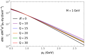
Figure 4: Thermal dilepton yields in the presence of collisional terms for different values of $Q\equiv\hat{q}/{T^{3}}$ and for invariant mass $M=1$ GeV. Equilibrium contribution to the dilepton yield ($\delta f=0$) is also plotted for comparison.

Fig. 4 shows the dilepton yields in presence of collisional terms as a function of transverse momentum $p_{T}$ for $M=1$ GeV. The yields are plotted for different values of the jet-quenching parameter, $\hat{q}/T^{3}\equiv Q$. It is observed that the presence of collisional terms increases the dilepton yield considerably, compared to the equilibrium case (represented by $\delta f=0$). Note that, with $Q=10$, there is an increase of $\sim 31.8\%$ at $p_{T}=1.5$ GeV and $\sim 145\%$ at $p_{T}=2.5$ GeV for $M=1$ GeV. It can be noted that the increment due to collisional terms decreases with the increase of $Q$. For $M=1$ GeV and at $p_{T}=2$ GeV, we observe $\sim 46\%$ enhancement in the yield with $Q=20$ and $\sim 30\%$ with $Q=30$. We observe that the effect of collisional terms is more prominent in the high $p_{T}$ regime, which indicates that these non-equilibrium effects are more dominant at high $p_{T}$. This is due to the fact that high $p_{T}$ particles are produced predominantly during the initial stages of QGP evolution. In the case of lower $p_{T}$, we observe a marginal decrease in the yields, which is indicative of the fact that these effects remain significant throughout the evolution of the plasma.

Now, we study the strength of these collisional effects to the equilibrium dilepton yield by constructing a ratio as given below,

$$R_{p_{T}}=\left[1+\frac{dN_{\chi}}{dM^{2}d^{2}p_{T}dy}/\frac{dN_{0}}{dM^{2}d^{2}p_{T}dy}\right].$$ (65)

Fig. 5 shows $R_{p_{T}}$ as a function of transverse momentum for various values of $Q$. We observe that the strength of collisional contributions are higher at large $p_{T}$ compared to lower $p_{T}$. As expected, we see a gradual increase in the collisional effects as we move towards high $p_{T}$. This trend remains the same for all values of $M$. It is observed that the strength of collisional corrections decreases with increase in $Q$. At low $p_{T}$, $R_{p_{T}}$ is less than unity, which indicates that the corrections suppress the particle spectra at lower $p_{T}$ and the maximum suppression can be seen for $Q=10$ and minimum for $Q=30$.

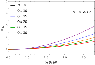
Figure 5: Strength of collisional terms to the equilibrium dilepton yield for various values of $Q$ with invariant mass $M=0.5$ GeV.

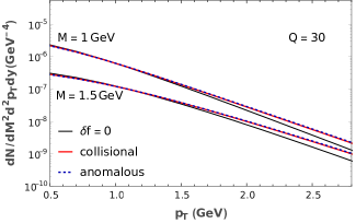
Figure 6: Thermal dilepton yields in the presence of collisional and anomalous corrections with $Q=30$, for different values of $M$.

Next, we compare the dilepton yields obtained for collisional and anomalous corrections in Fig. 6. In doing so, we plot the yields for $M=1,1.5$ GeV while fixing $Q=30$. Though the strength of non-equilibrium collisional effects on spectra is appreciable at high $p_{T}$, it is found to be lesser compared to that of the anomalous transport. We note that, over entire $p_{T}$, the effect due to anomalous transport is more compared to the collisional case. At $p_{T}=2.5$ GeV and with $M=1$ GeV, we observe $\sim 48.8\%$ increase in the yield in the presence of collisional effects, while for the same parameters the increment is $\sim 54.8\%$ for the anomalous case.

Fig. 7 shows the dilepton yields for collisional and anomalous corrections as a function of transverse momentum for $M=2$ GeV with different $Q$ values. Though, the effect of both the corrections is to increase the equilibrium dilepton yield at large $p_{T}$, the enhancement is found to be lesser when collisional terms are included. It is to be noted that difference between the two corrections is visibly observed for high $p_{T}$ and small $Q$. Our analysis indicates that the dilepton yield in the presence of collisional terms is lesser when compared to the collisionless anomalous transport case. This is in line with the argument of Ref. Asakawa:2006jn that the $2\rightarrow 2$ elastic collisions have only marginal contributions to transport coefficients as compared to that from the turbulent chromo fields described through effective Vlasov-Boltzmann equation.

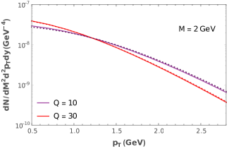
Figure 7: Thermal dilepton yields in the presence of collisional terms for different values of $Q\equiv\hat{q}/{T^{3}}$ and for invariant mass $M=2$ GeV. The dotted lines indicate yields from the anomalous transport only.

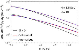
Figure 8: The effect of medium modified mass $M_{eff}$ on the thermal dilepton yields in the presence of collisional and anomalous corrections. The yields are plotted for $Q=10$ and $M=1.5$ GeV. The dashed lines indicate the yields obtained for the case $M_{eff}\rightarrow M$.

In Fig. 8, we plot the thermal dilepton yields in the presence of collisional and anomalous corrections observed for $M=1.5$ GeV and $Q=10$. Corresponding yields obtained in the $M_{eff}\rightarrow M$ limit are also plotted for comparison. As expected, we observe that the medium interaction effects suppress the spectra throughout the entire $p_{T}$ range compared to the $M_{eff}\rightarrow M$ limit. It can be seen that the difference between collisional and anomalous corrections at large $p_{T}$ is more visible when medium interaction effects are included. As the strength of momentum anisotropy varies with the evolution of medium, our results have a strong dependence on the temperature of the medium, time scale of instability in the medium and the choice of jet quenching parameter. It must be noted that the results presented here incorporate the effects of medium interactions on the cross-section, whereas in Ref. Chandra:2016dwy , these effects were not considered while calculating the dilepton spectra in the presence of anomalous transport.

In the present analysis, the collisional corrections to the thermal dilepton spectra are calculated using $(1+1)-$D Bjorken flow. It is to be noted that, in general, the Bjorken model tends to overestimate the particle production yields as the evolution time of the QGP is high compared to a three-dimensional flow. Also, we have not incorporated Debye screening corrections to thermal dilepton rates, since its effect is found to be minimal Chatterjee:1994dq in the current analysis. A quantitative study of collisional term correction to the spectra can be done by employing a $(2+1)-$D hydrodynamic flow and also including contributions from radiative processes/inelastic collisions. Moreover, apart from the dominant source considered, there are other higher-order processes that can also contribute to the thermal dilepton production Altherr:1992th ; Thoma:1997dk ; Burnier:2015rka ; Jackson:2019yao . It would be interesting to incorporate contributions from such channels along with the collisional corrections. This will be taken up for explorations in the near future.

VI Conclusion and outlook

In conclusion, we have estimated the thermal dilepton production rate while incorporating the collisional effects of the QGP medium along with the anomalous contributions. We have employed an effective Vlasov-Boltzmann equation to describe the dynamics of the medium in the presence of turbulent fields. The Vlasov term of the transport equation describes the evolution of distribution function with turbulent chromo-fields, whereas the collision kernel quantifies the effects of collisional processes in the rate of change of distribution function. We have analyzed the effect of these non-equilibrium corrections in thermal dilepton production from $q\overline{q}$ annihilation. The effects of the collisional processes in the presence of turbulent fields to the dilepton production rate are quantified in the case of $(1+1)-$D boost invariant expansion of the medium in the heavy-ion collision scenario.

The non-equilibrium effects are found to have a visible impact on the dilepton spectra. The effect of collisional corrections is to enhance the yield at high $p_{T}$, while it suppress the equilibrium dilepton spectra at lower $p_{T}$. Collisional effects in the dilepton production rate and yield are seen to have a strong dependence on the jet-quenching parameter ($Q\equiv\hat{q}/T^{3}$). Notably, the enhancement to the spectra is large for small $Q$ values. Further, we have analyzed the dependence of invariant mass $M$ to the collisional corrections to the dilepton production rate. In addition to this, the interplay of collisional processes and anomalous transport in the QGP medium is analysed through its strength on the dilepton production rates. The inclusion of collisional terms in the presence of chromo-turbulent fields suppressed the yield contribution from collisionless anomalous transport; and the difference is found to be more prominent in the high $p_{T}$ regime of the spectra. Moreover, we have analyzed the effects of medium interactions on the cross-section and studied its impact on thermal dilepton spectra in the presence of both collisional and anomalous corrections. The inclusion of medium effects has a significant impact on the yields, and it is found to suppress the dilepton spectra throughout the entire $p_{T}$ regime.

We intend to study the impact of collisional processes with both shear and bulk viscous effects on thermal dilepton spectra in heavy-ion collisions by employing a $(2+1)$-D hydrodynamical expansion of the system in the near future. Investigating the dilepton production rate in the magnetized QGP is another interesting direction to focus while utilizing the effective models for hot magnetized QCD medium Kurian:2017yxj . We leave these aspects for future works.

References

• (1) J. Adams et al. (STAR collaboration), Nucl. Phys. A 757, 102 (2005); K. Adcox et al. (PHENIX Collaboration), Nucl. Phys. A 757 184 (2005); B. Back et al. (PHOBOS Collaboration), Nucl. Phys. A 757, 28 (2005); A. Arsence et al. (BRAHMS Collaboration), Nucl. Phys. A 757, 1 (2005).
• (2) K. Yagi, T. Hatsuda and Y. Miake, Quark-Gluon Plasma: From Big Bang to Little Bang, Cambridge University Press, (2005).
• (3) P. F. Kolb and U. Heinz, “Hydrodynamic description of ultra-relativistic heavy-ion collisions,” in Quark-Gluon Plasma 3 (World Scientific, 2004) Chap. 10, pp. 634–714.
• (4) A. Muronga, Phys. Rev. C 69, 034903 (2004).
• (5) P. Romatschke and U. Romatschke, Phys. Rev. Lett.  99, 172301 (2007).
• (6) C. Gale, S. Jeon and B. Schenke, Int. J. Mod. Phys. A 28, 1340011 (2013).
• (7) P. Romatschke and U. Romatschke, doi:10.1017/9781108651998 arXiv:1712.05815 [nucl-th].
• (8) T. Hirano and M. Gyulassy, Nucl. Phys. A 769, 71 (2006).
• (9) T. H. Dupree, Phys. Fluids 9, 1773 (1966).
• (10) M. Asakawa, S. A. Bass and B. Muller, Phys. Rev. Lett.  96, 252301 (2006).
• (11) T. Abe and K. Niu, J. Phys. Soc. Jpn. 49 (1980), 717; T. Abe and K. Niu, J. Phys. Soc. Jpn. 49 (1980), 725.
• (12) T. Okada, T. Yabe, and K. Niu, J. Plasma Phys. 20 (1978), 405.
• (13) A. Majumder, B. Muller and X. N. Wang, Phys. Rev. Lett.  99, 192301 (2007).
• (14) M. Asakawa, S. A. Bass and B. Muller, Prog. Theor. Phys.  116, 725 (2007).
• (15) S. Mitra and V. Chandra, Phys. Rev. D 94, no. 3, 034025 (2016).
• (16) M. Kurian and V. Chandra, Phys. Rev. D 99, no. 11, 116018 (2019).
• (17) E. L. Fienberg, Nuovo Cim. A 34, 391 (1976)
• (18) E. V. Shuryak, Phys. Lett. 78, 150 (1978)
• (19) L. D. McLerran, T. Toimela, Phys. Rev.  D31 (1985) 545.
• (20) K. Kajantie, J. I. Kapusta, L. D. McLerran et al., Phys. Rev.  D34 (1986) 2746.
• (21) R. Rapp and H. van Hees, Phys. Lett. B 753 (2016) 586.
• (22) J. Alam, B. Sinha and S. Raha, Phys. Rept.  273 (1996) 243.
• (23) J. Alam, S. Sarkar, P. Roy, T. Hatsuda and B. Sinha, Annals Phys.  286, 159 (2001).
• (24) T. Peitzmann and M. H. Thoma, Phys. Rept.  364, 175 (2002).
• (25) R. Rapp and J. Wambach, Adv. Nucl. Phys.  25 (2000) 1.
• (26) G. Vujanovic, C. Young, B. Schenke, R. Rapp, S. Jeon and C. Gale, Phys. Rev. C 89, no. 3, 034904 (2014).
• (27) K. Dusling and S. Lin, Nucl. Phys. A 809 (2008) 246.
• (28) J. R. Bhatt, H. Mishra and V. Sreekanth, Nucl. Phys. A 875 (2012) 181.
• (29) R. S. Bhalerao, A. Jaiswal, S. Pal and V. Sreekanth, Phys. Rev. C 88 (2013) 044911
• (30) V. Chandra and V. Sreekanth, Phys. Rev. D 92, no. 9, 094027 (2015).
• (31) G. Vujanovic, G. S. Denicol, M. Luzum, S. Jeon and C. Gale, Phys. Rev. C 98, no. 1, 014902 (2018).
• (32) G. Vujanovic, J. F. Paquet, C. Shen, G. S. Denicol, S. Jeon, C. Gale and U. Heinz, arXiv:1903.05078 [nucl-th].
• (33) B. Singh, J. R. Bhatt and H. Mishra, Phys. Rev. D 100, no. 1, 014016 (2019).
• (34) A. Das, N. Haque, M. G. Mustafa and P. K. Roy, Phys. Rev. D 99, no. 9, 094022 (2019).
• (35) A. Bandyopadhyay, C. A. Islam and M. G. Mustafa, Phys. Rev. D 94, no. 11, 114034 (2016).
• (36) S. Ghosh and V. Chandra, Phys. Rev. D 98, no. 7, 076006 (2018).
• (37) V. Chandra and V. Sreekanth, Eur. Phys. J. C 77, no. 6, 427 (2017).
• (38) J. R. Bhatt, H. Mishra and V. Sreekanth, JHEP 1011 (2010) 106.
• (39) V. Chandra and V. Ravishankar, Phys. Rev. D 84, 074013 (2011).
• (40) V. Chandra, R. Kumar and V. Ravishankar, Phys. Rev. C 76, 054909 (2007), Erratum: [Phys. Rev. C 76, 069904 (2007)].
• (41) V. Chandra and V. Ravishankar, Eur. Phys. J. C 59, 705 (2009).
• (42) S. Bhadury, M. Kurian, V. Chandra and A. Jaiswal, arXiv:1902.05285 [hep-ph].
• (43) S. Mitra and V. Chandra, Phys. Rev. D 97, no. 3, 034032 (2018).
• (44) S. Mitra and V. Chandra, Phys. Rev. D 96, no. 9, 094003 (2017).
• (45) M. Kurian, S. Mitra, S. Ghosh and V. Chandra, Eur. Phys. J. C 79, no. 2, 134 (2019).
• (46) M. Y. Jamal, I. Nilima, V. Chandra and V. K. Agotiya, Phys. Rev. D 97, no. 9, 094033 (2018).
• (47) A. Kumar, M. Y. Jamal, V. Chandra and J. R. Bhatt, Phys. Rev. D 97, no. 3, 034007 (2018).
• (48) P. B. Arnold, G. D. Moore and L. G. Yaffe, JHEP 0011, 001 (2000).
• (49) P. K. Srivastava, L. Thakur and B. K. Patra, Phys. Rev. C 91, no. 4, 044903 (2015).
• (50) N. Haque, M. G. Mustafa and M. Strickland, Phys. Rev. D 87, no. 10, 105007 (2013).
• (51) M. Laine and Y. Schroder, JHEP 0503, 067 (2005).
• (52) R. Vogt, Ultrarelativistic Heavy-Ion Collisions, Elsevier, (2007).
• (53) G. Domokos and J. I. Goldman, Phys. Rev. D 23, 203 (1981).
• (54) T. Song, W. Cassing, P. Moreau and E. Bratkovskaya, Phys. Rev. C 98, no.4, 041901 (2018).
• (55) M. Laine, JHEP 11, 120 (2013).
• (56) M. Laine, PoS CPOD2014, 065 (2015).
• (57) P. Aurenche, F. Gelis, G. D. Moore and H. Zaraket, JHEP 12, 006 (2002).
• (58) J. D. Bjorken, Phys. Rev.  D 27 (1983) 140.
• (59) M. Cheng et. al, Phys. Rev. D 77, 014511 (2008).
• (60) L. Chatterjee and Cheuk-Yin Wong, Phys. Rev. C 51, 2125 (1995).
• (61) T. Altherr and P. V. Ruuskanen, Nucl. Phys. B 380 (1992) 377.
• (62) M. H. Thoma and C. T. Traxler, Phys. Rev. D 56, 198 (1997).
• (63) Y. Burnier and C. Gastaldi, Phys. Rev. C 93, no. 4, 044902 (2016).
• (64) G. Jackson and M. Laine, JHEP 11, 144 (2019).
• (65) M. Kurian and V. Chandra, Phys. Rev. D 96, no. 11, 114026 (2017).