Parameterization and applications of the low-$Q^{2}$ nucleon vector form factors

Abstract

We present the proton and neutron vector form factors in a convenient parametric form that is optimized for momentum transfers $\lesssim$ few GeV². The form factors are determined from a global fit to electron scattering data and precise charge radius measurements. A new treatment of radiative corrections is applied. This parametric representation of the form factors, uncertainties and correlations provides an efficient means to evaluate many derived observables. We consider two classes of illustrative examples: neutrino–nucleon scattering cross sections at GeV energies for neutrino oscillation experiments and nucleon structure corrections for atomic spectroscopy. The neutrino–nucleon charged current quasielastic (CCQE) cross section differs by 3%–5% compared to commonly used form factor models when the vector form factors are constrained by recent high-statistics electron–proton scattering data from the A1 Collaboration. Nucleon structure parameter determinations include: the magnetic and Zemach radii of the proton and neutron, $[r_{M}^{p},r_{M}^{n}]=[0.739(41)(23),0.776(53)(28)]$ fm and $[r_{Z}^{p},r_{Z}^{n}]=[1.0227(94)(51),-0.0445(14)(3)]$ fm; the Friar radius of nucleons, $[(r^{p}_{F})^{3},(r^{n}_{F})^{3}]=[2.246(58)(2),0.0093(6)(1)]$ ${\rm fm}^{3}$; the electric curvatures, $[\langle r^{4}\rangle^{p}_{E},\langle r^{4}\rangle^{n}_{E}]=[1.08(28)(5),-0.33(24)(3)]$ ${\rm fm}^{4}$; and bounds on the magnetic curvatures, $[\langle r^{4}\rangle^{p}_{M},\langle r^{4}\rangle^{n}_{M}]=[-2.0(1.7)(0.8),-2.3(2.1)(1.1)]$ ${\rm fm}^{4}$. The first and dominant uncertainty is propagated from the experimental data and radiative corrections, and the second error is due to the fitting procedure.

1 Introduction

A new generation of precision measurements, including accelerator-based neutrino experiments and muonic atom spectroscopy, demands a rigorous assessment of nucleon structure parameters and their uncertainties. The electromagnetic form factors of the proton and neutron are critical inputs to searches for new physical phenomena and to new precise measurements of the elementary particles. As one example, precise neutrino–nucleus interaction cross sections are required in order to access fundamental neutrino properties at long-baseline oscillation experiments [1, 2, 3]; the electroweak vector form factors of the nucleons are an important input to these cross sections, and are determined by an isospin rotation of the electromagnetic form factors. As another example, muonic atom spectroscopy [4, 5] has opened a new window on the determination of fundamental constants, and has revealed surprising discrepancies in comparisons of different approaches to nucleon structure [6]; it is critical to quantify uncertainties of nucleon structure inputs for the muonic atom program and also to incorporate constraints from these new measurements into other processes, such as the above-mentioned neutrino cross sections.

Recently, with Ye and Arrington [7], two of us provided a new global fit of the proton and neutron electromagnetic form factors, encompassing the entire momentum transfer ($Q^{2}$) range of available elastic electron scattering data. That analysis provides a comprehensive discussion of the available data, and the fit provides a general purpose tool for studying the form factors over a broad range of $Q^{2}$. However, the fit of Ref. [7] is not optimized for relatively low-$Q^{2}$ applications, such as neutrino scattering in the GeV energy regime. First, the inclusion of very high-$Q^{2}$ data necessitates the introduction of a large number of parameters, many of which are irrelevant to low-$Q^{2}$ applications. Second, the presentation of errors in Ref. [7] (an envelope around the curve as a function of $Q^{2}$) does not allow a systematic propagation of errors into derived observables. Finally, since the focus of Ref. [7] was in summarizing the implications of electron scattering data in isolation, it did not incorporate the low-$Q^{2}$ constraint on the proton electric form factor that emerges from muonic atom spectroscopy. While there is not a complete consensus regarding the resolution of the so-called proton radius puzzle [8, 9, 10, 11, 12], we believe it is important to be able to consistently incorporate these data and study their impact for applications such as neutrino scattering.

In this paper, we utilize the raw data selections and uncertainty evaluations for electron scattering cross sections from Ref. [7] to present a complete and compact parametric representation and covariance matrix for the form factors suitable for GeV and sub-GeV scale applications. Section 2 begins by describing the salient features of the data analysis and presenting the fit results. Section 3 considers several illustrative applications, beginning with a discussion of form factor radii and curvatures in Sec. 3.1. Section 3.2 evaluates neutrino–nucleon scattering cross sections. Section 3.3 presents central values and uncertainties for several nucleon structure parameters that are important for muonic atom spectroscopy. Section 4 provides a summary discussion. Appendix A discusses tensions between datasets. Appendix B provides details on the dispersive evaluation of two-photon exchange radiative corrections. Appendix C compares our numerical results for nucleon structure parameters to previous estimates.

2 Presentation of form factors

In this section, we begin by recalling definitions and conventions, discuss our data selection and fit procedure, and present the fit results.

2.1 Definitions

The Dirac and Pauli form factors, $F^{N}_{1}$ and $F^{N}_{2}$, respectively, are defined as matrix elements of the electromagnetic current:

$$\langle N(p^{\prime})|J_{\mu}^{\rm em}|N(p)\rangle=\bar{u}(p^{\prime})\left[\gamma_{\mu}\tilde{F}^{N}_{1}(Q^{2})+\frac{i\sigma_{\mu\nu}}{2M_{N}}\tilde{F}^{N}_{2}(Q^{2})q^{\nu}\right]u(p)\,,$$ (1)

where $q^{\mu}=p^{\prime\mu}-p^{\mu}$, $Q^{2}=-q^{2}=-(p^{\prime}-p)^{2}$, and $N$ stands for $p$ (proton) or $n$ (neutron). In the presence of radiative corrections, the on-shell form factors $\tilde{F}_{i}$ are IR divergent, and we define IR finite form factors $F_{i}(Q^{2})\equiv F_{i}(Q^{2},\mu=M_{p})$ in the $\overline{\rm MS}$ scheme at the renormalization scale $\mu=M_{p}$ [13]. We will present results in terms of the Sachs electric and magnetic form factors, which are related to the Dirac-Pauli basis by

$$G^{N}_{E}=F^{N}_{1}-\frac{Q^{2}}{4M_{N}^{2}}F^{N}_{2}\,,\quad G^{N}_{M}=F^{N}_{1}+F^{N}_{2}\,.$$ (2)

For some applications, it is convenient to work with the isoscalar and isovector linear combinations,

$$G_{E}^{S}=G_{E}^{p}+G_{E}^{n}\,,\quad G_{E}^{V}=G_{E}^{p}-G_{E}^{n}\,.$$ (3)

The form factors can be expressed as a convergent expansion in the variable $z(Q^{2})$ [14, 15, 16],

$$G_{E}^{N}(Q^{2})=\sum_{k=0}^{k_{\max}}a_{k}z(Q^{2})^{k}\,,\quad G_{M}^{N}(Q^{2})=G_{M}(0)\sum_{k=0}^{k_{\max}}b_{k}z(Q^{2})^{k}\,,\quad z(Q^{2})=\frac{\sqrt{t_{\mathrm{cut}}+Q^{2}}-\sqrt{t_{\mathrm{cut}}-t_{0}}}{\sqrt{t_{\mathrm{cut}}+Q^{2}}+\sqrt{t_{\mathrm{cut}}-t_{0}}}\,.$$ (4)

The dimensionless coefficients $a_{k}$, $b_{k}$ in this expansion encode hadronic structure. The parameter $t_{\mathrm{cut}}$ is the timelike kinematic threshold for particle production: $t_{\mathrm{cut}}=9m_{\pi}^{2}$ for isoscalar form factors and $t_{\mathrm{cut}}=4m_{\pi}^{2}$ for isovector form factors. The parameter $t_{0}$ represents the point in the $Q^{2}$ plane mapping to $z=0$; this free parameter defines the expansion scheme and is chosen for convenience. For example, the choice of $t_{0}$ that ensures the smallest range of $|z|$ corresponding to $0<Q^{2}<Q^{2}_{\rm max}$ is

$$t_{0}^{\mathrm{opt}}(t_{\mathrm{cut}},Q^{2}_{\max})=t_{\mathrm{cut}}(1-\sqrt{1+Q^{2}_{\max}/t_{\mathrm{cut}}})\,.$$ (5)

Perturbative QCD requires that the form factors fall off faster than $1/Q^{3}$ in the large $Q^{2}$ limit [17], which implies the four sum rules [16]

$$\sum_{k=n}^{\infty}k(k-1)\cdots(k-n+1)a_{k}=0\,,\qquad n=0,1,2,3\,.$$ (6)

It will also be useful to consider the small-$Q^{2}$ expansion of the form factors, written conventionally as

$$G^{N}_{E}(Q^{2}) = G^{N}_{E}(0)-\frac{\langle r^{2}\rangle^{N}_{E}}{3!}Q^{2}+\frac{\langle r^{4}\rangle^{N}_{E}}{5!}Q^{4}+\cdots\,,$$ (7)

$$G^{N}_{M}(Q^{2}) = G^{N}_{M}(0)\Bigg{(}1-\frac{\langle r^{2}\rangle^{N}_{M}}{3!}Q^{2}+\frac{\langle r^{4}\rangle^{N}_{M}}{5!}Q^{4}+\cdots\Bigg{)}\,.$$ (8)

We further define $r_{E}^{N}=\sqrt{\langle r^{2}\rangle^{N}_{E}}$ and $r_{M}^{N}=\sqrt{\langle r^{2}\rangle^{N}_{M}}$.

2.2 Data selection

For elastic $ep$- and $en$-scattering measurements, a complete tabulation of the data and error assignments that we use can be found in the supplemental material of Ref. [7]. We provide a short synopsis here. The $ep$-scattering data are divided into three datasets:

1. “Mainz”: the rebinned 2010 data from the A1 experiment [19] with modifications as detailed in Ref. [16], which comprise 657 data points in the kinematic range $Q^{2}<1\,\mathrm{GeV}^{2}$;

2. “World”: the compilation of unpolarized cross-section data not contained in the “Mainz” dataset [20, 21, 22, 23, 24, 25, 26, 27, 28, 29, 30, 31, 32, 33, 34, 35, 36, 37, 38, 39, 40, 41, 42, 43, 44, 45, 46, 47, 19];

3. “Pol”: $G_{E}^{p}/G_{M}^{p}$ ratios extracted from polarization data [48, 49, 50, 51, 52, 53, 54, 55, 56, 57, 58, 59, 60].

For $en$ scattering, we include all data available from Refs. [61, 62, 63, 64, 65, 66, 67, 68, 69, 70, 71, 72, 73, 74, 75] for $G_{E}^{n}$ and Refs. [76, 77, 78, 79, 80, 81, 82] for $G_{M}^{n}$. As explained in detail in Appendix A.2, we do not include PRad data to the fit since complete uncertainty correlations are not yet available [83].

In addition to electron scattering data, we include precision low-$Q^{2}$ constraints on the form factors. Charge conservation requires that $G_{E}^{p}(0)=1$ and $G_{E}^{n}(0)=0$. The magnetic moments of the proton and neutron determine [6] (see also Ref. [84]) $G_{M}^{p}(0)\equiv\mu_{p}/(e\hbar/2M_{p})=2.7928473508(85)$ and $G_{M}^{n}(0)\equiv\mu_{n}/(e\hbar/2M_{n})=-1.91304272(45)\times(M_{n}/M_{p})$. The proton electric charge radius can be inferred from the measurement of the 2$S$–2$P$ Lamb shift in muonic hydrogen [4]; we employ the updated value [5]

$$\left(r_{E}^{p}\right)_{\mu\mathrm{H}}=0.84087(39)\text{ fm}\,.$$ (9)

The neutron electric charge radius is determined from neutron scattering length measurements on heavy targets [85, 86], which yield

$$\langle r^{2}\rangle^{n}_{E}=-0.1161(22)\text{ fm}^{2}\,.$$ (10)

We do not include external constraints on $r_{M}^{p}$ or $r_{M}^{n}$. We have not included dispersive constraints [87, 88, 11, 12] on the form factors such as from $\pi\pi\to N\bar{N}$ data, since these constraints have either modest impact on the fits [14] or introduce further theoretical considerations. Our form factor results are presented with complete error budgets that may be compared to other determinations using dispersive analysis, lattice QCD or future electron scattering data.

Fit	$Q^{2}_{\max}$ [GeV2]	Mainz	World	Pol	$G_{E}^{n}$	$G_{M}^{n}$	$r_{E}^{p}$	$\langle r^{2}\rangle_{E}^{n}$	$\chi^{2}\quad$	$n_{\rm dof}$
$p$	1.0	657	0	0	0	0	1	0	475.35	650
$n$ ($G_{E}^{n}$)	1.0	0	0	0	29	0	0	1	14.81	26
$n$ ($G_{M}^{n}$)	1.0	0	0	0	0	15	0	0	8.03	11
iso $(1\,{\rm GeV}^{2})$	1.0	657	0	0	29	15	1	1	499.63	687
iso $(3\,{\rm GeV}^{2})$	3.0	657	480	58	37	23	1	1	1162.45	1241

Table 1: Number of data points from each dataset included in fits below the momentum transfer $Q^{2}_{\mathrm{max}}$. The total $\chi^{2}$ and number of degrees of freedom of each fit are also displayed.

We will consider two types of fits: first, a fit of separate proton and neutron data to their respective form factors; second, a fit of combined proton and neutron data to isospin-decomposed form factors. For our default proton fit (line 1 of Table 1), we employ the “Mainz” $ep$-scattering dataset in combination with the proton electric charge radius. For our default neutron fit (lines 2 and 3 of Table 1), we consider $en$-scattering data with $Q^{2}\leq 1\,{\rm GeV}^{2}$ in combination with the neutron electric charge radius. For our default isospin-decomposed fit (line 4 of Table 1), we consider all of the above proton and neutron data. Finally, we also consider an isospin-decomposed fit (line 5 of Table 1) that includes all of the above data, as well as neutron data with $1\,{\rm GeV}^{2}<Q^{2}\leq 3\,{\rm GeV}^{2}$, and “World” and “Pol” data with $0<Q^{2}\leq 3\,{\rm GeV}^{2}$. The total number of data points for each of these fits is summarized in Table 1. We also show the total $\chi^{2}$ and number of degrees of freedom for each fit.

2.3 Radiative corrections to $ep$ scattering

One goal of the current work is a more robust accounting for radiative corrections to unpolarized $ep$ cross sections in the fits. Besides the standard QED corrections on the electron line, there are three types of radiative corrections that must be applied to scattering data in order to extract the IR finite “Born” form factors defined after Eq. (1). They may be classified as “hadronic vertex”, “hadronic vacuum polarization” and “two-photon exchange” (TPE). The first, hadronic vertex, type of correction involves soft radiation and the shape of the event distribution as a function of the inelasticity $\Delta E=E_{e}^{\prime\,\rm elastic}-E_{e}^{\prime}$ (where $E_{e}^{\prime}$ is the scattered electron energy and $E_{e}^{\prime\,\rm elastic}$ is the elastic limit). This correction is calculable from QED in the soft limit $\Delta E\ll m_{\pi}$, but is numerically enhanced by large logarithms in that limit. In the Mainz data, the soft-photon tail was analyzed in detail but neglected higher-order corrections that are larger than stated systematic uncertainties [13]; however, the bulk of these corrections is absorbed by floating normalization parameters. In the World data, uncorrelated uncertainties were included in the dataset [7] to account for possible model dependence in the treatment of the radiative tail. In all cases, the error budgets from Ref. [7] are assumed to contain any residual error from the approximate treatment of this correction; we include here the small discrepancy between the $\overline{\rm MS}$ convention defined after Eq. (1), and the commonly used Maximon–Tjon convention [91] for the soft subtraction (see Appendix B of Ref. [13] for related discussion). The second, hadronic vacuum polarization, type of correction was omitted from the Mainz dataset [19], and treated nonuniformly in the World dataset. As with the hadronic vertex correction, the error budgets from Ref. [7] are assumed to contain any residual error from approximate treatment of this correction (see Sec. 1 of Ref. [16] for related discussion).

The third, TPE type of correction, remains a significant contributor to the error budget for $ep$ scattering. As with the hadronic vertex correction, the soft-photon part of the TPE correction is computable without uncertainty in QED, while the remaining hard-photon part is removed according to

$$d\sigma^{\rm Born} =\frac{d\sigma^{\rm expt}}{1+\delta_{\rm TPE}}\,.$$ (11)

Here $d\sigma^{\rm expt}$ is the experimental cross section after extracting leptonic QED corrections, and the above-mentioned hadronic vertex, vacuum polarization, and soft-photon TPE effects. The resultant $d\sigma^{\rm Born}$ is identified with the tree-level (Mott) cross section computed using Born form factors.

At arbitrary $Q^{2}$, we account for differences between the true TPE correction and the previous default model employed in Ref. [7], called there “SIFF Blunden” [92], by writing (for notational simplicity, we henceforth suppress the subscript “TPE” on $\delta$)

$$\begin{split}\delta&=\begin{cases}\delta^{\rm default}+x\,(\delta^{\rm dispersive}-\delta^{\rm default})&Q^{2}<1\,\mathrm{GeV}^{2}\\ \delta^{\rm default}+y\,\delta^{\rm AMT}&Q^{2}>1\,\mathrm{GeV}^{2}\end{cases}\,.\end{split}$$ (12)

For data below $Q^{2}=1\,{\rm GeV}^{2}$, we consider the dispersive analysis from Refs. [93, 94, 95, 96, 97, 98], which determines $\delta=\delta^{\rm dispersive}$; details are provided in Appendix B. We take the discrepancy between the default model and the dispersive analysis as an uncertainty and allow $x=1\pm 1$. Above $Q^{2}=1$ GeV², we consider the phenomenological correction from Ref. [90], $\delta=\delta^{\rm default}+y\delta^{\rm AMT}$, which is designed to improve agreement between polarization measurements and TPE-corrected unpolarized Rosenbluth measurements at high $Q^{2}$; the explicit form of $\delta^{\rm AMT}$ is provided in Appendix B. We take the discrepancy between the default model and this phenomenological ansatz as an uncertainty and conservatively allow $y=1\pm 2$. Since the ansatz involving $\delta^{\rm AMT}$ is purely phenomenological, we perform fits with $y=1\pm 2$ enforced as an uncorrelated error, as in Ref. [7], whereas $x=1\pm 1$ is enforced as a correlated error. We have verified that taking $x$ uncorrelated or $y$ correlated does not significantly alter the results. As a practical summary, our treatment of radiative corrections follows Ref. [7] above $Q^{2}=1\,{\rm GeV}^{2}$, with the additional parameter $x$ to describe TPE corrections below $Q^{2}=1\,{\rm GeV}^{2}$.

2.4 Fit parameters and procedure

form factor	$t_{\mathrm{cut}}$ [GeV2]	$t_{0}$ [GeV2]	$k_{\max}-4$	$|a_{k}|_{\max}$
$G_{E}^{p},G_{M}^{p}$	$4m_{\pi}^{2}$	$-0.21$	$4$	5
$G_{E}^{n},G_{M}^{n}$	$4m_{\pi}^{2}$	$-0.21$	$4$	5
$G_{E}^{S},G_{M}^{S}$	$9m_{\pi}^{2}$	$-0.28$	$4$	5
$G_{E}^{V},G_{M}^{V}$	$4m_{\pi}^{2}$	$-0.21$	$4$	5

Table 2: Parameter choices for the $z$ expansion of the form factors in this paper. Throughout the paper, we use the charged pion mass $m_{\pi}=0.13957$ GeV for the evaluation of $t_{\rm cut}$. The values for $t_{0}$ are obtained by rounding $t_{0}^{\mathrm{opt}}(1\,\mathrm{GeV}^{2};4m_{\pi}^{2})\approx-0.21$, and $t_{0}^{\mathrm{opt}}(1\,\mathrm{GeV}^{2};9m_{\pi}^{2})\approx-0.28$.

Having defined our datasets and treatment of radiative corrections, let us determine the relevant parameters for the $z$-expansion analysis. We use data with $Q^{2}\leq 1$ GeV² for our default fits, and choose $t_{0}$ as in Eq. (5) to minimize the maximum size of $|z|$ in this $Q^{2}$ range. We enforce sum rules on the coefficients, fix the normalization of form factors at zero momentum transfer, and choose the number of free parameters in the $z$ expansion, $n_{\rm max}=k_{\rm max}-4=4$, sufficiently large so that terms of order $|z|^{n_{\rm max}+1}$ are small compared to experimental precision. Our results do not change significantly when $k_{\rm max}$ is increased; we illustrate this in Sec. 3 by recomputing observables using $k_{\rm max}\to k_{\rm max}+1$. For all form factors, we have enforced Gaussian bounds, $|a_{k}|\leq 5$, $|b_{k}|\leq 5$ ($k=1,\dots,k_{\rm max}$) on the coefficients (i.e., a term $a_{k}^{2}/5^{2}$ is included in the $\chi^{2}$ function). Our results do not change significantly when this bound is increased by a factor of 2. In Table 2, we summarize the choices of $z$-expansion parameters used in our fits. For each choice of dataset in Table 1, the fit returns form factors expressed as central values, errors, and correlations for the indicated number of free parameters.

2.5 Fit results

For the proton fit (line 1 of Table 1), the form factor coefficients are

$$\begin{split}[a^{p}_{1},a^{p}_{2},a^{p}_{3},a^{p}_{4}]&=[-1.4860(97),-0.096(52),1.82(15),1.29(41)]\,,\\ [b^{p}_{1},b^{p}_{2},b^{p}_{3},b^{p}_{4}]&=[-1.464(11),0.063(60),1.74(21),-0.35(38)]\,.\end{split}$$ (13)

For the neutron fits (lines 2 and 3 of Table 1), the form factor coefficients are

$$\begin{split}[a^{n}_{1},a^{n}_{2},a^{n}_{3},a^{n}_{4}]&=[0.084(18),-0.279(63),-0.15(32),0.35(56)]\,,\\ [b^{n}_{1},b^{n}_{2},b^{n}_{3},b^{n}_{4}]&=[-1.415(39),0.22(17),1.39(39),0.0(1.5)]\,.\end{split}$$ (14)

For the isospin-decomposed fit (line 4 of Table 1), the isovector form factor coefficients are

$$\begin{split}[a^{V}_{1},a^{V}_{2},a^{V}_{3},a^{V}_{4}]&=[-1.576(15),0.177(77),2.05(24),0.88(57)]\,,\\ [b^{V}_{1},b^{V}_{2},b^{V}_{3},b^{V}_{4}]&=[-1.456(13),0.186(67),1.63(23),-0.73(46)]\,,\end{split}$$ (15)

and the isoscalar form factors are given by

$$\begin{split}[a^{S}_{1},a^{S}_{2},a^{S}_{3},a^{S}_{4}]&=[-1.809(17),0.91(12),1.92(27),-0.98(82)]\,,\\ [b^{S}_{1},b^{S}_{2},b^{S}_{3},b^{S}_{4}]&=[-1.938(57),0.78(25),3.71(88),-4.0(2.8)]\,.\end{split}$$ (16)

Whereas in Ref. [7] we considered the most inclusive dataset, here we have chosen the default proton dataset to contain the most recent precise measurements and to minimize internal data tensions. For definiteness we have included neutron data up to the same $Q^{2}_{\rm max}=1\,{\rm GeV}^{2}$. We remark that the Mainz dataset predicts $r_{E}^{p}=0.879(18)\,{\rm fm}$ when the $\mu$H charge radius constraint is removed [16]; this value is in only mild tension, $2.2\,\sigma$, with Eq. (9). The absence of more severe internal data tensions does not guarantee the absence of potentially underestimated systematics; for a fuller discussion we refer to Ref. [16].

Plots in Appendix A compare our $G_{E}^{p},G_{M}^{p}$, $G_{E}^{n},G_{M}^{n}$, and $G_{E}^{V},G_{M}^{V}$ form factors against those of our previous global fit in Ref. [7] and to the BBBA2005 parameterization of Ref. [99]. In Supplemental Material, we provide values for the coefficients and covariance matrices suitable for precise evaluation of charge radii and other physical quantities,as well as values for the coefficients from a fit with $k_{\mathrm{max}}=9$ which we use in applications to estimate the error from $z$-expansion truncation.

3 Illustrative applications

Having determined the form factor coefficients, errors and correlations, let us illustrate with some relevant physical examples. We begin in Sec. 3.1 by evaluating form factor radii and curvatures. Section 3.2 discusses neutrino scattering applications and Sec. 3.3 considers nucleon structure parameters for atomic spectroscopy.

3.1 Form factor radii and curvatures

Table 3: Electric and magnetic radii of proton and neutron using form factor parameters and bounds of Table 2 and datasets of Table 1. For $r_{M}$, the second number in each table results from changing the default $k_{\rm max}=8$ to $k_{\rm max}=9$.

Fit choice	$r_{E}^{p}$ $[\mathrm{fm}]$	$r^{p}_{M}$ $[\mathrm{fm}]$	$\langle r^{2}\rangle^{n}_{E}$ $[\mathrm{fm^{2}}]$	$r^{n}_{M}$ $[\mathrm{fm}]$
$p$	$0.84089(39)$	$0.739(41)$, $0.716(44)$	—	—
$n\,(G_{E}^{n})$	—	—	$-0.1161(22)$	—
$n\,(G_{M}^{n})$	—	—	—	$0.881(83)$, $0.878(79)$
iso (1 GeV2)	$0.84090(39)$	$0.749(36)$, $0.729(38)$	$-0.1160(22)$	$0.776(53)$, $0.748(57)$
iso (3 GeV2)	$0.84097(39)$	$0.799(23)$, $0.819(25)$	$-0.1160(22)$	$0.821(34)$, $0.855(38)$

Table 4: Same as Table 3, but for curvatures.

Fit	$\langle r^{4}\rangle^{p}_{E}$ $[\mathrm{fm^{4}}]$	$\langle r^{4}\rangle^{p}_{M}$ $[\mathrm{fm^{4}}]$	$\langle r^{4}\rangle^{n}_{E}$ $[\mathrm{fm^{4}}]$	$\langle r^{4}\rangle^{n}_{M}$ $[\mathrm{fm^{4}}]$
$p$	$1.08(28)$, $1.13(30)$	$-2.0(1.7)$, $-2.8(1.8)$	—	—
$n\,(G_{E}^{n})$	—	—	$-0.37(62)$, $-0.35(63)$	—
$n\,(G_{M}^{n})$	—	—	—	$1.6(3.3)$, $1.4(3.3)$
iso (1 GeV2)	$1.25(23)$, $1.21(23)$	$-1.6(1.5)$, $-2.4(1.5)$	$-0.33(24)$, $-0.30(25)$	$-2.3(2.1)$, $-3.4(2.2)$
iso (3 GeV2)	$0.83(18)$, $0.78(19)$	$-0.6(9)$, $0.6(1.2)$	$0.04(20)$, $0.08(21)$	$-1.1(1.3)$, $0.8(1.7)$

The nucleon radii, defined in Eqs. (7) and (8), are presented in Table 3, where each line represents the result of the fit using the corresponding dataset in Table 1. For each entry in the table, the first number represents the fit with default $k_{\rm max}=8$ (as in Table 2), and the second number represents the fit with $k_{\rm max}=9$.

As expected, the output proton and neutron electric radii are driven by the precise external constraints on these quantities and the $k_{\rm max}$ dependence is insignificant and not displayed. The determination of $r_{E}^{p}$ using low-$Q^{2}$ data released in 2019 by the PRad experiment is discussed in Appendix A.

The proton and neutron magnetic radii are consistent between fits, and represent the best values for these quantities obtained from electron scattering data plus external charge radius constraints. The proton magnetic radius from the default fit, $r_{M}^{p}=0.739(41)(23)\,{\rm fm}$, should be compared to (and does not essentially alter) our previous extraction from 2010 Mainz data, $r_{M}^{p}=0.776(34)(17)\,{\rm fm}$. The difference results from omitting the muonic hydrogen constraint of Eq. (9), omitting the floating TPE correction in Eq. (12), omitting sum rule constraints on the coefficients, and restricting to $Q^{2}_{\rm max}=0.5\,{\rm GeV}^{2}$. The neutron magnetic radius from our default fit, $r_{M}^{n}=0.776(53)(28)\,{\rm fm}$, represents a new extraction. Our value may be compared to the result $0.89(3)\,{\rm fm}$ from Ref. [101] that performed a $z$-expansion fit to $ep$ and $en$ scattering data and $\pi\pi\to N\bar{N}$ data, utilizing a dataset for $G_{M}^{p}$ from Ref. [90] that did not include 2010 Mainz data. The PDG recommended value $r_{M}^{n}=0.864(9)\,{\rm fm}$ [100] results from a naive average of this result and the result $r_{M}^{n}=0.862(9)\,{\rm fm}$ from Ref. [87] that performed a global fit of spacelike and timelike data to model spectral functions.

The form factor curvatures, $\langle r^{4}\rangle$ from Eqs. (7) and (8), are presented in Table 4. Only the proton electric curvature is determined to be nonzero with statistical significance. As for the radii, different fit variations are consistent within uncertainties. We provide previous estimates of curvature in Table 10 of Appendix C.

For both radii and curvatures, the iso (1 GeV²) fit yields a modest reduction in uncertainty compared to the separate proton and neutron fits, which can be traced to more data and a higher threshold $t_{\rm cut}$ (hence a smaller range of $|z|$ and a smaller number of relevant form factor coefficients) in the isoscalar channel. There is further reduction in the errors using the iso (3 GeV²) fit due to the inclusion of more data. As discussed in Appendix A, these additional data introduce a significant and unresolved tension with the Mainz dataset; we focus on the $p$, $n$ and iso ($1\,\mathrm{GeV}^{2}$) fits as our default results.

3.2 Neutrino–nucleon scattering

The elementary signal process for neutrino oscillation experiments is charged current quasielastic scattering,

$$\begin{split}\nu_{\ell}+n&\to\ell^{-}+p\,\\ \bar{\nu}_{\ell}+p&\to\ell^{+}+n\,.\end{split}$$ (17)

Neglecting power corrections to four-fermion theory of order $Q^{2}/M_{W}^{2}$ ($M_{W}$ is the $W^{\pm}$ boson mass), the cross section in the laboratory frame is

$$\frac{d\sigma}{dQ^{2}}(Q^{2},E_{\nu})=\frac{G_{F}^{2}|V_{ud}|^{2}}{8\pi}\frac{M^{2}}{E_{\nu}^{2}}\left[A(Q^{2})\frac{m_{\ell}^{2}+Q^{2}}{M^{2}}-B(Q^{2})\frac{s-u}{M^{2}}+C(Q^{2})\left(\frac{s-u}{M^{2}}\right)^{2}\right]\,,$$ (18)

where $G_{F}$ is the Fermi constant, $V_{ud}$ is a Cabibbo–Kobayashi–Maskawa (CKM) matrix element, $M=(M_{p}+M_{n})/2$ is the average nucleon mass, $m_{\ell}$ is the final-state lepton mass, $E_{\nu}$ is the incoming neutrino energy, and the difference in Mandelstam variables can be written as $s-u=4E_{\nu}M-Q^{2}-m_{\ell}^{2}$. The three structure-dependent functions $A,~{}B$, and $C$ are given by

$$\begin{split}A&=2\tau_{N}(F_{1}^{V}+F_{2}^{V})^{2}-(1+\tau_{N})\Big{[}(F_{1}^{V})^{2}+\tau_{N}(F_{2}^{V})^{2}-(F_{A})^{2}\Big{]}\\ &\quad-r_{\ell}^{2}\left[(F_{1}^{V}+F_{2}^{V})^{2}+\left(F_{A}+2F_{P}\right)^{2}-4(1+\tau_{N})F_{P}^{2}\right]\,,\\ B&=4\tau_{N}F_{A}(F_{1}^{V}+F_{2}^{V})\,,\\ C&=\frac{1}{4}\left[(F_{1}^{V})^{2}+\tau_{N}(F_{2}^{V})^{2}+(F_{A})^{2}\right]\,,\end{split}$$ (19)

where $\tau_{N}=Q^{2}/(4M^{2}),r_{\ell}=m_{\ell}/(2M)$, and the four form factors $F_{1}^{V},F_{2}^{V},F_{A},F_{P}$ are defined by

$$\langle p(p^{\prime})|\bar{u}\gamma^{\mu}P_{L}d|n(p)\rangle=\frac{1}{2}\bar{u}^{(p)}(p^{\prime})\!\left[\gamma^{\mu}F_{1}^{V}(Q^{2})+\frac{i\sigma^{\mu\nu}q_{\nu}}{2M}F_{2}^{V}(Q^{2})+\gamma^{\mu}\gamma_{5}F_{A}(Q^{2})+\frac{q^{\mu}}{M}\gamma_{5}F_{P}(Q^{2})\right]\!u^{(n)}(p)\,,$$ (20)

with $P_{L}=(1-\gamma_{5})/2$. Equation (18) represents the “Born” cross section for the quasielastic process, analogous to Eq. (11) for the case of $ep$ scattering. Soft radiation effects and two-boson exchange contributions have been subtracted and are to be treated separately. It is important to include such radiative corrections and to account for collinear and hard-photon emission in a practical experiment [104, 105, 106, 13]; however, our focus here is to determine the Born cross section for the quasielastic process.

The axial form factor $F_{A}$ is taken from Ref. [107]. In order to illustrate the utility of the new vector form factors, we will use the standard partially-conserved axial current (PCAC) ansatz for the pseudoscalar form factor $F_{P}$ (whose effects are suppressed by powers of the lepton mass),

$$F_{P}(Q^{2}) =\frac{2M^{2}}{m_{\pi}^{2}+Q^{2}}F_{A}(Q^{2})\,.$$ (21)

The isovector vector form factors $F_{1}^{V}$ and $F_{2}^{V}$ are determined either by taking the difference of proton and neutron form factors, or by directly implementing the isospin-decomposed fit. We have ignored second-class form factors in Eq. (20), and isospin-violating corrections to the relation of $F_{i}^{p,n}$ to $F_{i}^{V}$. These effects are suppressed by the fine structure constant $\alpha$ or by $(m_{d}-m_{u})/\Lambda_{\rm QCD}$, and are expected to be small compared to other uncertainties.

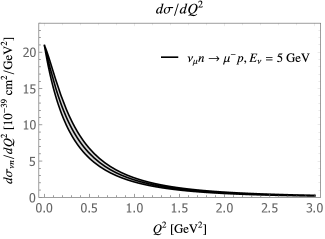
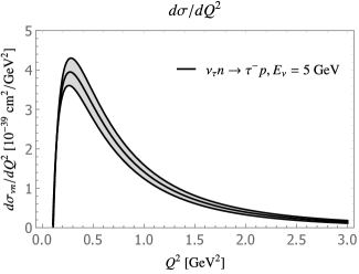
Figure 1: Neutrino–neutron quasielastic scattering cross section versus $Q^{2}$ for muon [left] and tau [right] flavors, using the iso (1 GeV²) fit.

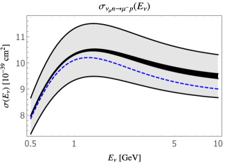
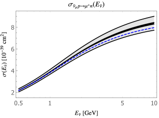
Figure 2: Muon neutrino–neutron [left] and antineutrino–proton [right] quasielastic cross section. Our result is given by the narrow dark band representing the iso (1 GeV²) fit with vector form factor uncertainty. Axial form factor uncertainty is represented by the wide light band and is to be added in quadrature. The blue dashed line represents the central value using the same axial form factor as the central curve, but BBBA2005 vector form factors.

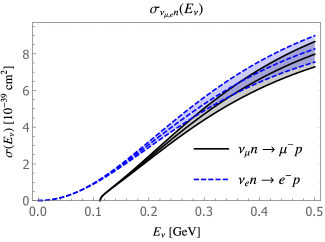
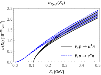
Figure 3: Electron and muon neutrino–neutron [left] and antineutrino–proton [right] quasielastic cross section at low energies. The shaded regions correspond to the light bands in Fig. 2. The region with solid boundary line represents the $\nu_{\mu}$ case and the region with dotted boundary line represents the $\nu_{e}$ case. The vector form factor uncertainty from our fit is not resolved in the plots.

To illustrate the relevant range of $Q^{2}$ for neutrino beams in the GeV energy regime, we display the $\nu_{\mu}n$ charged-current quasielastic (CCQE) cross section as a function of $Q^{2}$, fixing $E_{\nu}=5~{}\mathrm{GeV}$, in the left-hand side of Fig. 1. The cross section is dominated by $Q^{2}\lesssim 1$ GeV², and is relatively insensitive to the detailed form factor behavior at larger momentum transfers. For comparison, the right-hand side of Fig. 1 shows the $\nu_{\tau}n$ CCQE cross section; this rare process accesses somewhat larger $Q^{2}$. In both cases, there can be residual sensitivity to higher-order coefficients in the $z$ expansion that are poorly constrained by the chosen electron scattering dataset. This sensitivity can be determined in practice by recomputing observables using different values of $k_{\rm max}$.

Our CCQE cross sections for muon (anti)neutrino are displayed as a function of neutrino energy in Fig. 2, using our default isospin-decomposed (iso 1 GeV²) fit. The current large uncertainty of the axial form factor dominates the error budget. We remark that the deviation of central values between our fit and the commonly used BBBA2005 model [99] is sizable compared to the axial form factor uncertainty at $E_{\nu}\gtrsim 1\,{\rm GeV}$. The cross section depends strongly on lepton flavor at energies near or below the muon-production threshold, as shown in Fig. 3.

Table 5: CCQE cross section at $E_{\nu}=0.5$ GeV. Errors are from axial form factor $(A)$, vector form factors [$(V)$ for isospin-decomposed fits or $(p)$ and $(n)$ for separate proton and neutron fits], and $z$-expansion truncation ($t$).

Fit choice	$\sigma_{\nu_{\mu}n\xrightarrow{}\mu^{-}p}$ $[10^{-39}\,\mathrm{cm^{2}}]$	$\sigma_{\bar{\nu}_{\mu}p\xrightarrow{}\mu^{+}n}$ $[10^{-39}\,\mathrm{cm^{2}}]$
$p,n$	$7.971(689)_{A}(7)_{p}(16)_{n}(0.2)_{t}$	$2.196(146)_{A}(2)_{p}(5)_{n}(0.3)_{t}$
iso (1 GeV2)	$7.975(689)_{A}(17)_{V}(1)_{t}$	$2.197(146)_{A}(4)_{V}(0.5)_{t}$
iso (3 GeV2)	$7.958(689)_{A}(15)_{V}(7)_{t}$	$2.186(146)_{A}(4)_{V}(0.2)_{t}$
BBBA	$7.87(69)_{A}(8)_{V}$	$2.18(15)_{A}(8)_{V}$

Table 6: Same as for Table 7, but for $E_{\nu}=1$ GeV.

Fit choice	$\sigma_{\nu_{\mu}n\xrightarrow{}\mu^{-}p}$ $[10^{-39}\,\mathrm{cm^{2}}]$	$\sigma_{\bar{\nu}_{\mu}p\xrightarrow{}\mu^{+}n}$ $[10^{-39}\,\mathrm{cm^{2}}]$
$p,n$	$10.312(987)_{A}(11)_{p}(22)_{n}(5)_{t}$	$3.886(220)_{A}(5)_{p}(8)_{n}(3)_{t}$
iso (1 GeV2)	$10.319(988)_{A}(24)_{V}(6)_{t}$	$3.887(220)_{A}(9)_{V}(3)_{t}$
iso (3 GeV2)	$10.200(981)_{A}(20)_{V}(3)_{t}$	$3.851(225)_{A}(7)_{V}(1)_{t}$
BBBA	$10.10(98)_{A}(18)_{V}$	$3.82(23)_{A}(8)_{V}$
Ref. [107]	$10.1(9)$	$3.83(23)$

Table 7: Same as for Table 7, but for $E_{\nu}=3$ GeV.

Fit choice	$\sigma_{\nu_{\mu}n\xrightarrow{}\mu^{-}p}$ $[10^{-39}\,\mathrm{cm^{2}}]$	$\sigma_{\bar{\nu}_{\mu}p\xrightarrow{}\mu^{+}n}$ $[10^{-39}\,\mathrm{cm^{2}}]$
$p,n$	$10.035(935)_{A}(31)_{p}(66)_{n}(69)_{t}$	$6.686(461)_{A}(19)_{p}(34)_{n}(38)_{t}$
iso (1 GeV2)	$10.061(936)_{A}(71)_{V}(77)_{t}$	$6.699(460)_{A}(39)_{V}(43)_{t}$
iso (3 GeV2)	$9.710(918)_{A}(19)_{V}(3)_{t}$	$6.515(471)_{A}(13)_{V}(2)_{t}$
BBBA	$9.61(91)_{A}(24)_{V}$	$6.45(47)_{A}(15)_{V}$
Ref. [107]	$9.6(9)$	$6.47(47)$

Tables 7, 7 and 7 show the CCQE total cross sections for three benchmark points with $E_{\nu}=0.5,1$, and $3$ GeV. In addition to axial and vector form factor uncertainties, we include a $z$-expansion truncation uncertainty estimated from the shift in central value when the default fit with $k_{\rm max}=8$ is replaced by the fit with $k_{\rm max}=9$. We also compare our evaluation with Ref. [107], where the BBBA2005 parameterization was used for vector form factors.

3.3 Spectroscopy of electronic and muonic atoms

Modern spectroscopy experiments with ordinary and muonic hydrogen [108, 109, 110, 4, 5, 111, 112, 113] are sensitive to the internal structure of the proton. In particular, the small size of muonic atoms enhances sensitivity to structure-dependent effects and makes measurements with muons attractive in searches for new physics and precise studies of proton and nuclear dynamics. The leading structure-dependent effect, which is proportional to $\langle r^{2}\rangle_{E}$, shifts energy levels at order $m_{\ell}\alpha^{4}$ and enters via the exchange of one virtual photon between the lepton ($\ell=e$ or $\ell=\mu$) and the proton. This effect does not depend on the spin state of the energy level. The leading spin-dependent contribution of order $m_{\ell}\alpha^{5}$ arises from the two-photon exchange. It contributes to the hyperfine splitting of energy levels [5]. Modern measurements of the Lamb shift in muonic hydrogen [4, 5], of the hydrogen-deuterium isotope shift [114] and of the $1S$–$2S$ transition in hydrogen [115] are sensitive to spin-independent two-photon exchange contributions as well. For both ordinary and muonic hydrogen, the bulk of the two-photon exchange contributions is determined by certain structure parameters, “moments”, expressed as $Q^{2}$ integrals over products of elastic form factors. In this section, we compute the Friar and Zemach radii governing spin-independent and spin-dependent two-photon exchange, respectively. Some previous results are compiled in Appendix C.

3.3.1 Lamb shift

The leading structure-dependent contribution to the Lamb shift in hydrogen is proportional to the (cube of the) Friar radius $r_{F}$:

$$r_{F}^{3}=\frac{24}{\pi}\int_{0}^{\infty}\frac{dQ^{2}}{Q^{5}}\left[G_{E}^{2}(Q^{2})-1-2Q^{2}G_{E}^{\prime}(0)\right]\,,$$ (22)

where $G_{E}^{\prime}(0)=dG_{E}/dQ^{2}|_{Q^{2}=0}$. We evaluate $r_{F}^{3}$ exploiting the fit of proton and neutron data as well as isospin-decomposed fits and present our results in Table 8. The first error is from the extracted form factor covariance matrix, and the second is the shift in central value when the default fit with $k_{\rm max}=8$ is replaced by the fit with $k_{\rm max}=9$. We note that removing the $\mu$H constraint from our default proton fit shifts $(r^{p}_{F})^{3}=2.246(58)\,{\rm fm}^{3}\to 2.97(35)\,{\rm fm}^{3}$.

Table 8: Friar radii of proton and neutron. The first error is from the extracted form factor covariance matrix and the second error is from $z$-expansion truncation.

Fit choice	$\left(r_{F}^{p}\right)^{3}~{}[\mathrm{fm}^{3}]$	$\left(r_{F}^{n}\right)^{3}~{}[\mathrm{fm}^{3}]$
$p,n$	$2.246(58)(2)$	$0.0093(11)(1)$
iso (1 GeV2)	$2.278(49)(12)$	$0.0093(6)(1)$
iso (3 GeV2)	$2.176(38)(10)$	$0.0100(5)(0)$

3.3.2 Hyperfine splitting

The first measurements of the $1S$ hyperfine splitting in muonic hydrogen with ppm precision are being planned by the CREMA [111] and FAMU [112] Collaborations, and at J-PARC [113]. The leading nucleon-structure contribution to the hyperfine splitting of $S$ energy levels is given by the two-photon exchange diagram. The bulk of the correction is proportional to the Zemach radius $r_{Z}$ [116], which can be expressed as a convolution of nucleon electric and magnetic form factors,

$$r^{N}_{Z}=-\frac{4}{\pi}\int_{0}^{\infty}\frac{dQ}{Q^{2}}\bigg{[}\frac{G^{N}_{M}(Q^{2})G^{N}_{E}(Q^{2})-G^{N}_{M}(0)G^{N}_{E}(0)}{G^{N}_{M}(0)}\bigg{]}\,.$$ (23)

Table 9: Same as Table 8 but for Zemach radii.

Fit choice	$\quad r^{p}_{Z}~{}[\mathrm{fm}]$	$\quad r^{n}_{Z}~{}[\mathrm{fm}]$
$p,n$	$1.0227(94)(51)$	$-0.0443(26)(1)$
iso (1 GeV2)	$1.0246(84)(40)$	$-0.0445(14)(3)$
iso (3 GeV2)	$1.0450(58)(45)$	$-0.0462(12)(0)$

Similar to the Friar radii, we present Zemach radii evaluated using the fits from Sec. 2.5 in Table 9. These results provide a first rigorous error estimate. We note that removing the $\mu$H constraint from our default proton fit shifts $r^{p}_{Z}=1.0227(94)\,{\rm fm}\to 1.0426(132)\,{\rm fm}$.

4 Summary

We have presented a compact representation of the proton and neutron vector form factors in terms of $z$-expansion coefficients, including central values, errors and correlations. The results can be used to evaluate both central values and error bars for many derived quantities that are sensitive to GeV and sub-GeV momentum transfers.

In our default fits we employed the following data: (i) the high-statistics Mainz dataset for $ep$ cross sections; (ii) $en$ elastic scattering data at momentum transfers $Q^{2}\leq 1\,{\rm GeV}^{2}$; and (iii) precise external constraints on the proton and neutron electric charge radii. We considered two types of fits to these data. First, we performed separate proton and neutron fits, i.e., proton data fit to proton form factors and neutron data fit to neutron form factors. Second, we performed a fit of both proton and neutron data to isospin-decomposed form factors. For proton structure observables, there is only a slight reduction in uncertainty when the proton fit is replaced by the isospin-decomposed fit; for simplicity we use the proton fit as our final result: $r_{M}^{p}=0.739(41)(23)\,{\rm fm}$; $\langle r^{4}\rangle^{p}_{E}=1.08(28)(5)\,{\rm fm}^{4}$; $\langle r^{4}\rangle^{p}_{M}=-2.0(1.7)(8)\,{\rm fm}^{4}$; $(r_{F}^{p})^{3}=2.246(58)(2)\,{\rm fm}^{3}$; $r_{Z}^{p}=1.0227(94)(51)\,{\rm fm}$. For neutron structure observables, the abundance and precision of proton data relative to neutron data lead to a significant reduction in uncertainty when using the isospin-decomposed fit; we thus use the isospin-decomposed fit as our final result: $r_{M}^{n}=0.776(53)(28)\,{\rm fm}$; $\langle r^{4}\rangle^{n}_{E}=-0.33(24)(3)\,{\rm fm}^{4}$; $\langle r^{4}\rangle^{n}_{M}=-2.3(2.1)(1.1)\,{\rm fm}^{4}$; $(r_{F}^{n})^{3}=0.0093(6)(1)\,{\rm fm}^{3}$; $r_{Z}^{n}=-0.0445(14)(3)\,{\rm fm}$. For the neutrino CCQE cross sections, only the isovector combination of vector form factors appears, and we thus use the cross section determined from isospin-decomposed form factors as our default result for the Born cross sections: $\sigma_{\nu_{\mu}n\xrightarrow{}\mu^{-}p}|_{E_{\nu}=0.5\,{\rm GeV}}=7.975(689)(17)(1)$, $\sigma_{\nu_{\mu}n\xrightarrow{}\mu^{-}p}|_{E_{\nu}=1\,{\rm GeV}}=10.319(988)_{A}(24)(6)$ and $\sigma_{\nu_{\mu}n\xrightarrow{}\mu^{-}p}|_{E_{\nu}=3\,{\rm GeV}}=10.061(936)_{A}(71)(77)$. We present the uncertainty coming from vector form factors and the truncation uncertainty as the last two errors, respectively, in results of this paragraph.

Significant tensions exist between the default dataset and other $ep$ data. In Ref. [7], we quantified this tension as a function of $Q^{2}$. Without knowing the source of discrepancy it remains unclear how to rigorously address this tension in the fit, and how to propagate it to derived observables. In this paper, we bypass this issue by focusing on the internally consistent default dataset, but present results for comparison also from the global fit that includes World and Pol data as in Table 1. This combined iso (3 GeV²) fit is similar to our global fit from Ref. [7]; the detailed comparison is discussed in Appendix A. The iso (3 GeV²) fit includes more data than our default fit and it is thus not surprising that this fit predicts smaller uncertainties in derived observables. However, the fit does not address internal dataset tensions and the iso (3 GeV²) uncertainties are likely underestimates.

A primary goal of this work is to provide a consistent framework for applications such as neutrino event generators to propagate form factor constraints and uncertainties into cross section predictions. The framework is readily adapted to new data. Our new precise vector form factors have small uncertainty but deviate significantly from commonly used parameterizations; such deviations become sizable compared to the dominant axial form factor uncertainty for larger neutrino energies. It is important to address these discrepancies with future experimental and/or lattice QCD data. We remark that the axial form factor was extracted under a specific (BBBA2005) assumption for the vector form factors. This ansatz can be justified given the current large uncertainty of elementary target neutrino data. However, correlations between vector and axial form factors should be accounted for when future more precise data become available.

Acknowledgements R.J.H. and G.L. thank J. Arrington and Z. Ye for many discussions and collaboration on Refs. [16, 7] which inspired the present work. Similarly, R.J.H. thanks M. Betancourt, R. Gran and A. Meyer for discussion and collaboration on Ref. [107]. The research of K.B., R.J.H. and O.T. supported by the U.S. Department of Energy, Office of Science, Office of High Energy Physics, under Award No. DE-SC0019095. Fermilab is operated by Fermi Research Alliance, LLC under Contract No. DE-AC02-07CH11359 with the U.S. Department of Energy. G.L. acknowledges support by the Samsung Science & Technology Foundation under Project No. SSTF-BA1601-07, a Korea University Grant, and the support of the U.S. National Science Foundation through Grant No. PHY-1719877. G.L. is grateful to the Technion–Israel Institute of Technology, the Fermilab theory group, and the Mainz Institute for Theoretical Physics (MITP) for hospitality and partial support during completion of this work. O.T. acknowledges the Fermilab theory group and the theory group of Institute for Nuclear Physics at Johannes Gutenberg-Universität Mainz for warm hospitality and support. The work of O.T. is supported by the Visiting Scholars Award Program of the Universities Research Association.

Appendix A Consistency between datasets

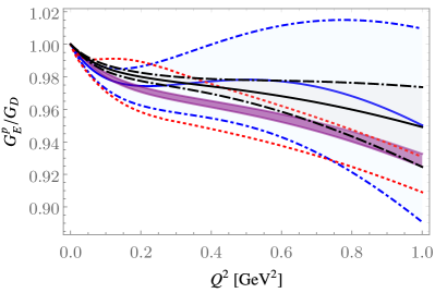
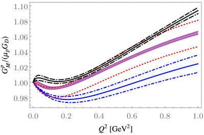
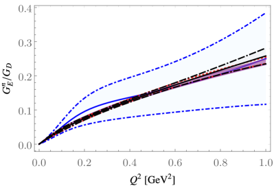
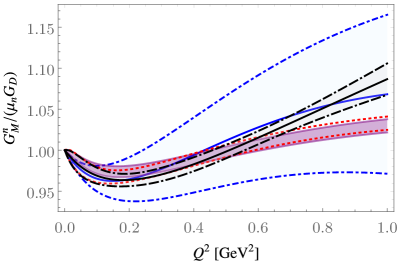
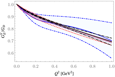
Figure 4: Plots of $1\sigma$ bands of $G_{E}^{p}$ and $G_{M}^{p}$ [top], $G_{E}^{n}$ and $G_{M}^{n}$ [middle], and $G_{E}^{V}$ and $G_{M}^{V}$ [bottom] from different fits. The black long dash-dotted curves are the results of the following: the $p$ fit of line 1 in Table 1 [top]; the $n$ fits of lines 2 and 3 in Table 1 [middle]; and the iso ($1\,\mathrm{GeV}^{2}$) fit of line 4 in Table 1 [bottom]. The purple bands are the results of the iso ($3\,\mathrm{GeV}^{2}$) fit of line 5 in Table 1. The red dotted curves correspond to the global fit of Ref. [7], and the blue dash-dotted curves are the BBBA2005 result of Ref. [99].

In this appendix, we discuss the tension between iso (1$~{}\mathrm{GeV^{2}}$) and iso (3$~{}\mathrm{GeV^{2}}$) fits and compare to our previous global fit [7] and to the BBBA2005 parameterization [99]. In particular, we illustrate the tension between extractions of $G_{M}^{p}$ at $Q^{2}\sim 1\,{\rm GeV}^{2}$ from the Mainz and other World cross-section data. This tension manifests in observables sensitive to moderate $Q^{2}\gtrsim{\rm few}\times 0.1\,{\rm GeV}^{2}$, such as CCQE cross sections with few GeV neutrino energies; cf. Fig. 2. We also show that including the PRad data does not significantly alter the fits when the $\mu$H constraint is imposed.

A.1 Mainz and World+Pol datasets

Figure 4 compares the form factors from our default $p$, $n$, and iso (1 GeV²) fits to our iso (3 GeV²) fit. We also compare to our previous global fit from Ref. [7]. That global fit corresponds with the iso (3 GeV²) fit after the following modifications: (i) inclusion of the $\mu$H constraint (9); (ii) improved treatment of TPE correction (12); (iii) omission of data above $Q^{2}=3\,{\rm GeV}^{2}$; (iv) choice of form factor expansion parameters $t_{0}$ and $k_{\rm max}$ optimized for $0<Q^{2}<1\,{\rm GeV}^{2}$. Note that the error band from Ref. [7] includes an ad hoc “data tension” error to account for the tension between Mainz and other World data. Since we have in mind applications to neutrino cross sections, we compare also to the commonly used BBBA2005 parameterization. The BBBA2005 parameterization resulted from a fit to data preceding the A1 experiment, and is in severe tension with our default fit for $G_{M}^{p}$.

A.2 PRad and Mainz datasets

The PRad Collaboration recently presented new measurements of elastic electron–proton scattering at JLAB [83]. At two beam energies $E=1.1\,\mathrm{GeV}$ and $2.2\,\mathrm{GeV}$, 33 and 38 measurements were taken in the range of $Q^{2}$ up to $0.016\,\mathrm{GeV}^{2}$ and $0.058\,\mathrm{GeV}^{2}$, respectively. PRad announced a result $r_{E}^{p}=0.831\pm 0.007_{\mathrm{stat}}\pm 0.012_{\mathrm{syst}}$ fm fitting to a rational functional form for $G_{E}^{p}$,

$$G_{E}^{p}(Q^{2})=\frac{1+p_{1}Q^{2}}{1+p_{2}Q^{2}}\,.$$ (24)

Notably, this is within $1\sigma$ of $\left(r_{E}^{p}\right)_{\mu\mathrm{H}}$ in Eq. (9) from muonic hydrogen spectroscopy.

The PRad Collaboration employed particular assumptions in fitting the cross sections, which are detailed in the supplementary material of Ref. [83]. To extract form factors, the measured scattering cross sections were fit to the following reduced cross section

$$\sigma^{\mathrm{red}}_{\mathrm{PRad}}=(nG_{E})^{2}+\frac{\tau}{\varepsilon}(G_{M}^{K})^{2}\,,$$ (25)

where $\tau=Q^{2}/(4M_{p}^{2})$, $\epsilon=[1+2(1+\tau)\tan^{2}(\theta/2)]^{-1}$, $n$ is a normalization parameter for a given beam energy, and $G_{M}^{K}$ is the Kelly parameterization for the proton magnetic form factor [117]. The PRad Collaboration showed that the cross sections vary by less than 0.2% when different models for the magnetic form factor are used.

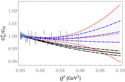
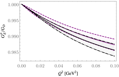
Figure 5: Comparison of $G_{E}^{p}$ from fits with and without PRad data. In both plots, the black, long dash-dotted curve is our default (proton) fit. On the left-hand side, blue points are the tabulated PRad form factors with statistical errors; the blue, dash-dotted curve is the PRad extraction; and the red, dotted curve is our extraction from PRad data. On the right-hand side, we compare our default fit to the fit when the $\mu$H constraint is replaced by PRad data (purple, dashed curve).

In Fig. 5, we compare $G_{E}^{p}$ from four fits:

1. (blue, dash-dotted curve in left plot) Fitting with the above rational functional form to the provided form factor tabulations with statistical-only errors, we have reproduced the PRad results for the proton charge radius and reduced $\chi^{2}$.

2. (red, dotted curve in left plot) Following a modified version of the PRad procedure, we also fit directly to the tabulated PRad cross sections with statistical and systematic uncertainties added in quadrature. Fixing the magnetic form factor to the dipole form $G_{M}^{p}(Q^{2})=\mu_{p}G_{D}(Q^{2})$, we employed the $z$ expansion (without sum rules) with $k_{\max}=3$ for $G_{E}^{p}$. For each beam energy, a separate normalization parameter multiplying the entire reduced cross section is used. We did not apply additional TPE corrections. The extracted radius value is $r_{E}^{p}=0.836(19)\,{\rm fm}$, with $\chi^{2}=23.88$ and $n_{\mathrm{dof}}=68$.

3. (black, long dash-dotted curve in both left and right plots) $G_{E}^{p}$ obtained from our default proton-only fit to Mainz data with $\left(r_{E}^{p}\right)_{\mu\mathrm{H}}$ constraint.

4. (purple, solid/dashed curve in right plot) $G_{E}^{p}$ obtained from the proton-only fit using the $z$ expansion with $k_{\mathrm{max}}=8$ to combined Mainz and PRad data (statistical and systematic uncertainties added in quadrature) without $\left(r_{E}^{p}\right)_{\mu\mathrm{H}}$ constraint. TPE corrections are applied to both datasets. The extracted radius value for this fit is $r_{E}^{p}=0.843(11)$ fm, with $\chi^{2}=503.24$ and $n_{\mathrm{dof}}=720$.

In the right plot of Fig. 5, we show that the combined fit without the $\mu$H constraint and our default fit with the $\mu$H constraint lie within the $1\sigma$ uncertainty bands of each other for the entire $Q^{2}$ range of the PRad data. It would be desirable to include the PRad data directly into our fits, alongside the data in Table 1; we refrain from doing so since the PRad uncertainties are systematics dominated and uncertainty correlations are not yet available [83]. We have shown, however, that these data will not significantly alter our fits once the precise external $\mu$H constraint is imposed. Taking the PRad errors at face value (i.e., neglecting correlations), we remark that the $z$-expansion fit to PRad data results in a significantly larger uncertainty for $r_{E}^{p}$ than is obtained using Eq. (24), comparable to the $\sim 0.020\,{\rm fm}$ uncertainty of our default proton fit, while the combined fit returns a radius uncertainty that is a factor of 2 smaller than either dataset in isolation.

Appendix B Two-photon exchange

In this appendix, we provide pertinent details of two-photon exchange corrections that were discussed in Section 2.3.

For momentum transfers $Q^{2}\lesssim 1\,\mathrm{GeV}^{2}$, dispersion relations have been used to constrain TPE corrections using available experimental data for inelastic cross sections. At relatively small momentum transfer and small scattering angles, the contribution from all inelastic intermediate states was evaluated [118] on top of the proton state [119] accounting for unpolarized proton inelastic structure functions in the resonance region. To calculate the TPE correction at large scattering angles, the data-driven dispersion relation framework was recently developed [93, 94, 95, 96, 97]. The imaginary part of TPE amplitudes is evaluated from on-shell information in the physical region of electron–proton scattering. The real part of TPE amplitudes requires information from the unphysical region as input. Novel methods of analytical continuation [94, 97] allow us to overcome this complication. Contributions from proton and $\pi N$ intermediate states are evaluated for $Q^{2}\lesssim 1\,\mathrm{GeV}^{2}$. At low momentum transfer and backward scattering angles, the relative contribution of inelastic intermediate states is found to be much smaller than the elastic contribution to TPE. At larger electron beam energies and momentum transfer, the intermediate states with higher invariant mass, e.g., $\pi\pi N$, become kinematically enhanced and prevent making a rigorous prediction in the absence of exclusive experimental data. At small momentum transfer $Q^{2}\lesssim 0.25\,\mathrm{GeV}^{2}$ and scattering angles, we account for all inelastic intermediate states [118]. At large angles and momentum transfer, proton and $\pi N$ states are included [94, 95, 97]. The intermediate region is described by interpolation between these two calculations as in Ref. [98]. We denote this dispersive result as $\delta^{\mathrm{dispersive}}$ and provide the corresponding correction for each point in the Mainz dataset in the Supplementary Material.

At larger momentum transfers, $Q^{2}\gtrsim 1\,\mathrm{GeV}^{2}$, the explicit form of the phenomenological TPE modification is as follows [90]:

$$\begin{split}\delta^{\mathrm{AMT}}(\varepsilon,~{}Q^{2})&=0.01(\varepsilon-1)\frac{\ln\frac{Q^{2}}{1\,\mathrm{GeV}^{2}}}{\ln 2.2}\,,\end{split}$$ (26)

which is negative (since $0\leq\varepsilon\leq 1$) and increases the inferred Born cross section. As discussed in the main text, this correction serves to improve agreement between polarization measurements and TPE-corrected unpolarized Rosenbluth measurements at high-$Q^{2}$.

Appendix C Comparison to literature

In this appendix, we provide some existent results for form factor curvatures, Friar radii and Zemach radii.

C.1 Curvature

The curvature of the proton form factor has been estimated by performing fits to data [120] and by performing calculations in heavy-baryon ChPT [121]. We tabulate these previous results in Table 10. Our extraction of electric curvature lies below previous extractions from data. The curvature of neutron form factors was evaluated in dispersively-improved chiral effective field theory (DI$\chi$EFT). Our results for the curvatures of both electric and magnetic neutron form factors are in a fair agreement with Ref. [122].

Table 10: Curvature of proton $(p)$ and neutron $(n)$ electromagnetic form factors.

Fit choice	$\langle r^{4}\rangle^{p}_{E}$ $[\mathrm{fm^{4}}]$	$\langle r^{4}\rangle^{p}_{M}$ $[\mathrm{fm^{4}}]$	$\langle r^{4}\rangle^{n}_{E}$ $[\mathrm{fm^{4}}]$	$\langle r^{4}\rangle^{n}_{M}$ $[\mathrm{fm^{4}}]$
This paper	$1.08(28)(5)$	$-2.0(1.7)(0.8)$	$-0.33(24)(3)$	$-2.3(2.1)(1.1)$
Heavy-baryon ChPT [121]	$0.60(29)$	$0.79(28)$	—	—
DI$\chi$EFT [122]	$1.47\cdots 1.60$	$1.68\cdots 1.78$	$-0.64\cdots-0.51$	$2.04$
Fit to data [123]	$1.53$	$0.91$	—	—
Based on A1 fits [120]	$2.31\cdots 2.64$	$-0.12\cdots 0.75$	—	—

C.2 Friar radius

We present some previous estimates of Friar radii in Table 11. There is a significant difference between results with and without the constraint on the proton charge radius [124, 125, 126, 127, 128, 129, 130, 131, 132, 133, 134, 88, 135, 136, 137].

Table 11: Friar radius of proton.

	$\left(r_{F}^{p}\right)^{3}~{}[\mathrm{fm}^{3}]$
This paper	$2.246(58)(2)$
Using A1 fits [128]	$2.85(8)$
Friar and Sick [136]	$2.71(13)$
Graczyk and Juszczak [137]	$2.889(8)$

C.3 Zemach radius

Previous results for the nucleon Zemach radii are $r^{p}_{Z}=1.045(4)~{}\mathrm{fm}$ in Ref. [128] for the proton and $r^{n}_{Z}=-0.0449(13)~{}\mathrm{fm}$ in Refs. [138, 139] for the neutron. These should be compared with our values: $r^{p}_{Z}=1.0227(94)(51)~{}\mathrm{fm}$ for the proton and $r^{n}_{Z}=-0.0445(14)(3)~{}\mathrm{fm}$ for the neutron. Further calculations and fits to scattering data are found in Refs. [125, 140, 141, 138, 142, 128, 137, 143]. Extractions from atomic spectroscopy are found in Refs. [5, 144, 145, 146, 147].

References

- Mosel [2016] U. Mosel, Ann. Rev. Nucl. Part. Sci. 66, 171 (2016), arXiv:1602.00696 [nucl-th].
- Katori and Martini [2018] T. Katori and M. Martini, J. Phys. G45, 013001 (2018), arXiv:1611.07770 [hep-ph].
- Alvarez-Ruso et al. [2018] L. Alvarez-Ruso et al., Prog. Part. Nucl. Phys. 100, 1 (2018), arXiv:1706.03621 [hep-ph].
- Pohl et al. [2010] R. Pohl et al., Nature 466, 213 (2010).
- Antognini et al. [2013] A. Antognini et al., Science 339, 417 (2013).
- Mohr et al. [2016] P. J. Mohr, D. B. Newell, and B. N. Taylor, Rev. Mod. Phys. 88, 035009 (2016), arXiv:1507.07956 [physics.atom-ph].
- Ye et al. [2018] Z. Ye, J. Arrington, R. J. Hill, and G. Lee, Phys. Lett. B777, 8 (2018), arXiv:1707.09063 [nucl-ex].
- Pohl et al. [2013] R. Pohl, R. Gilman, G. A. Miller, and K. Pachucki, Ann. Rev. Nucl. Part. Sci. 63, 175 (2013), arXiv:1301.0905 [physics.atom-ph].
- Carlson [2015] C. E. Carlson, Prog. Part. Nucl. Phys. 82, 59 (2015), arXiv:1502.05314 [hep-ph].
- Hill [2017a] R. J. Hill, Proceedings, 12th Conference on Quark Confinement and the Hadron Spectrum (Confinement XII): Thessaloniki, Greece, EPJ Web Conf. 137, 01023 (2017a), arXiv:1702.01189 [hep-ph].
- Alarcon et al. [2019] J. Alarcon, D. Higinbotham, C. Weiss, and Z. Ye, Phys. Rev. C 99, 044303 (2019), arXiv:1809.06373 [hep-ph].
- Hammer and Meissner [2020] H.-W. Hammer and U.-G. Meissner, Sci. Bull. 65, 257 (2020), arXiv:1912.03881 [hep-ph].
- Hill [2017b] R. J. Hill, Phys. Rev. D95, 013001 (2017b), arXiv:1605.02613 [hep-ph].
- Hill and Paz [2010] R. J. Hill and G. Paz, Phys. Rev. D82, 113005 (2010), arXiv:1008.4619 [hep-ph].
- Bhattacharya et al. [2011] B. Bhattacharya, R. J. Hill, and G. Paz, Phys. Rev. D84, 073006 (2011), arXiv:1108.0423 [hep-ph].
- Lee et al. [2015] G. Lee, J. R. Arrington, and R. J. Hill, Phys. Rev. D92, 013013 (2015), arXiv:1505.01489 [hep-ph].
- Lepage and Brodsky [1980] G. P. Lepage and S. J. Brodsky, Phys. Rev. D22, 2157 (1980).
- Friar [1979] J. L. Friar, Annals Phys. 122, 151 (1979).
- Bernauer et al. [2014] J. C. Bernauer et al. (A1), Phys. Rev. C90, 015206 (2014), arXiv:1307.6227 [nucl-ex].
- Dudelzak [1965] B. Dudelzak, Ph.D. thesis, University of Paris (1965).
- Janssens et al. [1966] T. Janssens, R. Hofstadter, E. B. Hughes, and M. R. Yearian, Phys. Rev. 142, 922 (1966).
- Bartel et al. [1966] W. Bartel et al., Phys. Rev. Lett. 17, 608 (1966).
- Albrecht et al. [1966] W. Albrecht et al., Phys. Rev. Lett. 17, 1192 (1966).
- Frèrejacque et al. [1966] D. Frèrejacque, D. Benaksas, and D. Drickey, Phys. Rev. 141, 1308 (1966).
- Albrecht et al. [1967] W. Albrecht et al., Phys. Rev. Lett. 18, 1014 (1967).
- Goitein et al. [1967] M. Goitein, J. R. Dunning, and R. Wilson, Phys. Rev. Lett. 18, 1018 (1967).
- Litt et al. [1970] J. Litt et al., Phys. Lett. B 31, 40 (1970).
- Goitein et al. [1970] M. Goitein et al., Phys. Rev. D 1, 2449 (1970).
- Berger et al. [1971] C. Berger et al., Phys. Lett. B 35, 87 (1971).
- Price et al. [1971] L. E. Price et al., Phys. Rev. D 4, 45 (1971).
- Ganichot et al. [1972] D. Ganichot, B. Grossetête, and D. Isabelle, Nucl. Phys. A 178, 545 (1972).
- Bartel et al. [1973] W. Bartel et al., Nucl. Phys. B 58, 429 (1973).
- Kirk et al. [1973] P. N. Kirk et al., Phys. Rev. D 8, 63 (1973).
- Borkowski et al. [1974] F. Borkowski et al., Nucl. Phys. A222, 269 (1974).
- Murphy et al. [1974] J. J. Murphy, Y. M. Shin, and D. M. Skopik, Phys. Rev. C 9, 2125 (1974).
- Borkowski et al. [1975] F. Borkowski et al., Nucl. Phys. B93, 461 (1975).
- Stein et al. [1975] S. Stein et al., Phys. Rev. D 12, 1884 (1975).
- Simon et al. [1980] G. G. Simon, C. Schmitt, F. Borkowski, and V. H. Walther, Nucl. Phys. A333, 381 (1980).
- Simon et al. [1981] G. G. Simon, C. Schmitt, and V. H. Walther, Nucl. Phys. A364, 285 (1981).
- Bosted et al. [1990] P. E. Bosted et al., Phys. Rev. C 42, 38 (1990).
- Rock et al. [1992] S. Rock et al., Phys. Rev. D 46, 24 (1992).
- Sill et al. [1993] A. F. Sill et al., Phys. Rev. D 48, 29 (1993).
- Walker et al. [1994] R. C. Walker et al., Phys. Rev. D 49, 5671 (1994).
- Andivahis et al. [1994] L. Andivahis et al., Phys. Rev. D 50, 5491 (1994).
- Dutta et al. [2003] D. Dutta et al., Phys. Rev. C 68, 064603 (2003).
- Christy et al. [2004] M. E. Christy et al. (E94110), Phys. Rev. C70, 015206 (2004), arXiv:nucl-ex/0401030 [nucl-ex].
- Qattan et al. [2005] I. A. Qattan et al., Phys. Rev. Lett. 94, 142301 (2005), arXiv:nucl-ex/0410010 [nucl-ex].
- Milbrath et al. [1998] B. D. Milbrath et al. (Bates FPP), Phys. Rev. Lett. 80, 452 (1998), [Erratum: Phys. Rev. Lett.82,2221(1999)], arXiv:nucl-ex/9712006 [nucl-ex].
- Pospischil et al. [2001] T. Pospischil et al. (A1), Eur. Phys. J. A12, 125 (2001).
- Gayou et al. [2001] O. Gayou et al., Phys. Rev. C64, 038202 (2001).
- Strauch et al. [2003] S. Strauch et al. (Jefferson Lab E93-049), Phys. Rev. Lett. 91, 052301 (2003), arXiv:nucl-ex/0211022 [nucl-ex].
- Punjabi et al. [2005] V. Punjabi et al., Phys. Rev. C71, 055202 (2005), [Erratum: Phys. Rev.C71,069902(2005)], arXiv:nucl-ex/0501018 [nucl-ex].
- MacLachlan et al. [2006] G. MacLachlan et al., Nucl. Phys. A764, 261 (2006).
- Jones et al. [2006] M. K. Jones et al. (Resonance Spin Structure), Phys. Rev. C74, 035201 (2006), arXiv:nucl-ex/0606015 [nucl-ex].
- Crawford et al. [2007] C. B. Crawford et al., Phys. Rev. Lett. 98, 052301 (2007), arXiv:nucl-ex/0609007 [nucl-ex].
- Ron et al. [2011] G. Ron et al. (Jefferson Lab Hall A), Phys. Rev. C84, 055204 (2011), arXiv:1103.5784 [nucl-ex].
- Zhan et al. [2011] X. Zhan et al., Phys. Lett. B705, 59 (2011), arXiv:1102.0318 [nucl-ex].
- Paolone et al. [2010] M. Paolone et al., Phys. Rev. Lett. 105, 072001 (2010), arXiv:1002.2188 [nucl-ex].
- Puckett et al. [2012] A. J. R. Puckett et al., Phys. Rev. C85, 045203 (2012), arXiv:1102.5737 [nucl-ex].
- Puckett et al. [2017] A. J. R. Puckett et al., Phys. Rev. C96, 055203 (2017), [erratum: Phys. Rev.C98,no.1,019907(2018)], arXiv:1707.08587 [nucl-ex].
- Meyerhoff et al. [1994] M. Meyerhoff et al., Phys. Lett. B327, 201 (1994).
- Eden et al. [1994] T. Eden et al., Phys. Rev. C50, R1749 (1994).
- Passchier et al. [1999] I. Passchier et al., Phys. Rev. Lett. 82, 4988 (1999), arXiv:nucl-ex/9907012 [nucl-ex].
- Herberg et al. [1999] C. Herberg et al., Eur. Phys. J. A5, 131 (1999).
- Rohe et al. [1999] D. Rohe et al., Phys. Rev. Lett. 83, 4257 (1999).
- Golak et al. [2001] J. Golak, G. Ziemer, H. Kamada, H. Witala, and W. Gloeckle, Phys. Rev. C63, 034006 (2001), arXiv:nucl-th/0008008 [nucl-th].
- Schiavilla and Sick [2001] R. Schiavilla and I. Sick, Phys. Rev. C64, 041002 (2001), arXiv:nucl-ex/0107004 [nucl-ex].
- Zhu et al. [2001] H. Zhu et al. (E93026), Phys. Rev. Lett. 87, 081801 (2001), arXiv:nucl-ex/0105001 [nucl-ex].
- Bermuth et al. [2003] J. Bermuth et al., Phys. Lett. B564, 199 (2003), arXiv:nucl-ex/0303015 [nucl-ex].
- Madey et al. [2003] R. Madey et al. (E93-038), Phys. Rev. Lett. 91, 122002 (2003), arXiv:nucl-ex/0308007 [nucl-ex].
- Warren et al. [2004] G. Warren et al. (Jefferson Lab E93-026), Phys. Rev. Lett. 92, 042301 (2004), arXiv:nucl-ex/0308021 [nucl-ex].
- Glazier et al. [2005] D. I. Glazier et al., Eur. Phys. J. A24, 101 (2005), arXiv:nucl-ex/0410026 [nucl-ex].
- Geis et al. [2008] E. Geis et al. (BLAST), Phys. Rev. Lett. 101, 042501 (2008), arXiv:0803.3827 [nucl-ex].
- Riordan et al. [2010] S. Riordan et al., Phys. Rev. Lett. 105, 262302 (2010), arXiv:1008.1738 [nucl-ex].
- Schlimme et al. [2013] B. S. Schlimme et al., Phys. Rev. Lett. 111, 132504 (2013), arXiv:1307.7361 [nucl-ex].
- Rock et al. [1982] S. Rock et al., New Horizons in Electromagnetic Physics, Charlottesville, Virginia, April 21-24, 1982, Phys. Rev. Lett. 49, 1139 (1982).
- Lung et al. [1993] A. Lung et al., Phys. Rev. Lett. 70, 718 (1993).
- Gao et al. [1994] H. Gao et al., Phys. Rev. C50, R546 (1994).
- Anklin et al. [1998] H. Anklin et al., Phys. Lett. B428, 248 (1998).
- Kubon et al. [2002] G. Kubon et al., Phys. Lett. B524, 26 (2002), arXiv:nucl-ex/0107016 [nucl-ex].
- Anderson et al. [2007] B. Anderson et al. (Jefferson Lab E95-001), Phys. Rev. C75, 034003 (2007), arXiv:nucl-ex/0605006 [nucl-ex].
- Lachniet et al. [2009] J. Lachniet et al. (CLAS), Phys. Rev. Lett. 102, 192001 (2009), arXiv:0811.1716 [nucl-ex].
- Xiong et al. [2019] W. Xiong et al., Nature 575, 147 (2019).
- Schneider et al. [2017] G. Schneider et al., Science 358, 1081 (2017).
- Kopecky et al. [1995] S. Kopecky, P. Riehs, J. A. Harvey, and N. W. Hill, Phys. Rev. Lett. 74, 2427 (1995).
- Kopecky et al. [1997] S. Kopecky, M. Krenn, P. Riehs, S. Steiner, J. A. Harvey, N. W. Hill, and M. Pernicka, Phys. Rev. C56, 2229 (1997).
- Belushkin et al. [2007] M. A. Belushkin, H. W. Hammer, and U. G. Meissner, Phys. Rev. C75, 035202 (2007), arXiv:hep-ph/0608337 [hep-ph].
- Lorenz et al. [2015] I. Lorenz, U.-G. Meissner, H.-W. Hammer, and Y. B. Dong, Phys. Rev. D 91, 014023 (2015), arXiv:1411.1704 [hep-ph].
- Arrington and Sick [2007] J. Arrington and I. Sick, Phys. Rev. C76, 035201 (2007), arXiv:nucl-th/0612079 [nucl-th].
- Arrington et al. [2007] J. Arrington, W. Melnitchouk, and J. A. Tjon, Phys. Rev. C76, 035205 (2007), arXiv:0707.1861 [nucl-ex].
- Maximon and Tjon [2000] L. C. Maximon and J. A. Tjon, Phys. Rev. C62, 054320 (2000), arXiv:nucl-th/0002058 [nucl-th].
- Blunden et al. [2005] P. G. Blunden, W. Melnitchouk, and J. A. Tjon, Phys. Rev. C72, 034612 (2005), arXiv:nucl-th/0506039 [nucl-th].
- Borisyuk and Kobushkin [2008] D. Borisyuk and A. Kobushkin, Phys. Rev. C78, 025208 (2008), arXiv:0804.4128 [nucl-th].
- Tomalak and Vanderhaeghen [2015] O. Tomalak and M. Vanderhaeghen, Eur. Phys. J. A51, 24 (2015), arXiv:1408.5330 [hep-ph].
- Tomalak et al. [2017a] O. Tomalak, B. Pasquini, and M. Vanderhaeghen, Phys. Rev. D95, 096001 (2017a), arXiv:1612.07726 [hep-ph].
- Blunden and Melnitchouk [2017] P. G. Blunden and W. Melnitchouk, Phys. Rev. C95, 065209 (2017), arXiv:1703.06181 [nucl-th].
- Tomalak et al. [2017b] O. Tomalak, B. Pasquini, and M. Vanderhaeghen, Phys. Rev. D96, 096001 (2017b), arXiv:1708.03303 [hep-ph].
- Tomalak [2018] O. Tomalak, Proceedings, 11th International Workshop on the Physics of Excited Nucleons (NSTAR 2017): Columbia, SC, USA, August 20-23, 2017, Few Body Syst. 59, 87 (2018), arXiv:1806.01627 [hep-ph].
- Bradford et al. [2006] R. Bradford, A. Bodek, H. S. Budd, and J. Arrington, NuInt05, proceedings of the 4th International Workshop on Neutrino-Nucleus Interactions in the Few-GeV Region, Okayama, Japan, 26-29 September 2005, Nucl. Phys. Proc. Suppl. 159, 127 (2006), arXiv:hep-ex/0602017 [hep-ex].
- Tanabashi et al. [2018] M. Tanabashi et al. (Particle Data Group), Phys. Rev. D98, 030001 (2018).
- Epstein et al. [2014] Z. Epstein, G. Paz, and J. Roy, Phys. Rev. D90, 074027 (2014), arXiv:1407.5683 [hep-ph].
- Llewellyn Smith [1972] C. H. Llewellyn Smith, Gauge Theories and Neutrino Physics, Jacob, 1978:0175, Phys. Rept. 3, 261 (1972).
- Kuzmin et al. [2008] K. S. Kuzmin, V. V. Lyubushkin, and V. A. Naumov, Eur. Phys. J. C54, 517 (2008), arXiv:0712.4384 [hep-ph].
- De Rujula et al. [1979] A. De Rujula, R. Petronzio, and A. Savoy-Navarro, Nucl. Phys. B 154, 394 (1979).
- Day and McFarland [2012] M. Day and K. S. McFarland, Phys. Rev. D86, 053003 (2012), arXiv:1206.6745 [hep-ph].
- Graczyk [2014] K. M. Graczyk, Phys. Lett. B732, 315 (2014), arXiv:1308.5581 [hep-ph].
- Meyer et al. [2016] A. S. Meyer, M. Betancourt, R. Gran, and R. J. Hill, Phys. Rev. D93, 113015 (2016), arXiv:1603.03048 [hep-ph].
- Beyer et al. [2017] A. Beyer et al., Science 358, 79 (2017).
- Fleurbaey et al. [2018] H. Fleurbaey, S. Galtier, S. Thomas, M. Bonnaud, L. Julien, F. Biraben, F. Nez, M. Abgrall, and J. Guena, Phys. Rev. Lett. 120, 183001 (2018), arXiv:1801.08816 [physics.atom-ph].
- Bezginov et al. [2019] N. Bezginov, T. Valdez, M. Horbatsch, A. Marsman, A. C. Vutha, and E. A. Hessels, Science 365, 1007 (2019).
- Pohl [2016] R. Pohl (CREMA), J. Phys. Soc. Jap. 85, 091003 (2016).
- Adamczak et al. [2016] A. Adamczak et al. (FAMU), JINST 11, P05007 (2016), arXiv:1604.01572 [physics.ins-det].
- Ma et al. [2016] Y. Ma et al., Proceedings, 21st International Symposium on Spin Physics (SPIN 2014): Beijing, China, October 20-24, 2014, Int. J. Mod. Phys. Conf. Ser. 40, 1660046 (2016).
- Parthey et al. [2010] C. G. Parthey, A. Matveev, J. Alnis, R. Pohl, T. Udem, U. D. Jentschura, N. Kolachevsky, and T. W. Hänsch, Phys. Rev. Lett. 104, 233001 (2010).
- Parthey et al. [2011] C. G. Parthey et al., Phys. Rev. Lett. 107, 203001 (2011), arXiv:1107.3101 [physics.atom-ph].
- Zemach [1956] A. C. Zemach, Phys. Rev. 104, 1771 (1956).
- Kelly [2004] J. J. Kelly, Phys. Rev. C70, 068202 (2004).
- Tomalak and Vanderhaeghen [2016] O. Tomalak and M. Vanderhaeghen, Phys. Rev. D93, 013023 (2016), arXiv:1508.03759 [hep-ph].
- Blunden et al. [2003] P. G. Blunden, W. Melnitchouk, and J. A. Tjon, Phys. Rev. Lett. 91, 142304 (2003), arXiv:nucl-th/0306076 [nucl-th].
- [120] J. Bernauer, “Coefficients for fits with polynomials of order 9,10,11,12,” based on private communication.
- Horbatsch et al. [2017] M. Horbatsch, E. A. Hessels, and A. Pineda, Phys. Rev. C95, 035203 (2017), arXiv:1610.09760 [nucl-th].
- Alarcón and Weiss [2018] J. M. Alarcón and C. Weiss, Phys. Lett. B784, 373 (2018), arXiv:1803.09748 [hep-ph].
- Barcus et al. [2020] S. K. Barcus, D. W. Higinbotham, and R. E. McClellan, Phys. Rev. C 102, 015205 (2020), arXiv:1902.08185 [physics.data-an].
- Friar and Payne [1997] J. L. Friar and G. L. Payne, Phys. Rev. C56, 619 (1997), arXiv:nucl-th/9704032 [nucl-th].
- Pachucki [1996] K. Pachucki, Phys. Rev. A53, 2092 (1996).
- Pachucki [1999] K. Pachucki, Phys. Rev. A60, 3593 (1999), arXiv:physics/9906002 [physics.atom-ph].
- Pineda [2005] A. Pineda, Phys. Rev. C71, 065205 (2005), arXiv:hep-ph/0412142 [hep-ph].
- Distler et al. [2011] M. O. Distler, J. C. Bernauer, and T. Walcher, Phys. Lett. B696, 343 (2011), arXiv:1011.1861 [nucl-th].
- De Rujula [2010] A. De Rujula, Phys. Lett. B693, 555 (2010), arXiv:1008.3861 [hep-ph].
- Cloet and Miller [2011] I. C. Cloet and G. A. Miller, Phys. Rev. C83, 012201 (2011), arXiv:1008.4345 [hep-ph].
- Wu and Kao [2011] B. Y. Wu and C. W. Kao, (2011), arXiv:1108.2968 [hep-ph].
- Indelicato [2013] P. Indelicato, Phys. Rev. A87, 022501 (2013), arXiv:1210.5828 [physics.atom-ph].
- Borie [2012] E. Borie, Annals Phys. 327, 733 (2012), arXiv:1103.1772 [physics.atom-ph].
- Peset and Pineda [2014] C. Peset and A. Pineda, Nucl. Phys. B887, 69 (2014), arXiv:1406.4524 [hep-ph].
- Karshenboim et al. [2015] S. G. Karshenboim, E. Yu. Korzinin, V. A. Shelyuto, and V. G. Ivanov, Phys. Rev. D91, 073003 (2015), arXiv:1501.06539 [hep-ph].
- Friar and Sick [2005] J. L. Friar and I. Sick, Phys. Rev. A72, 040502 (2005), arXiv:nucl-th/0508025 [nucl-th].
- Graczyk and Juszczak [2015] K. M. Graczyk and C. Juszczak, Phys. Rev. C91, 045205 (2015).
- Friar and Payne [2005a] J. L. Friar and G. L. Payne, Phys. Rev. C72, 014002 (2005a), arXiv:nucl-th/0504015 [nucl-th].
- Tomalak [2019] O. Tomalak, Phys. Rev. D99, 056018 (2019), arXiv:1812.03884 [nucl-th].
- Friar and Sick [2004] J. L. Friar and I. Sick, Phys. Lett. B579, 285 (2004), arXiv:nucl-th/0310043 [nucl-th].
- Friar and Payne [2005b] J. L. Friar and G. L. Payne, Phys. Lett. B618, 68 (2005b), arXiv:nucl-th/0502004 [nucl-th].
- Carlson et al. [2008] C. E. Carlson, V. Nazaryan, and K. Griffioen, Phys. Rev. A78, 022517 (2008), arXiv:0805.2603 [physics.atom-ph].
- Tomalak [2017] O. Tomalak, Eur. Phys. J. C77, 858 (2017), arXiv:1708.02509 [hep-ph].
- Dupays et al. [2003] A. Dupays, A. Beswick, B. Lepetit, C. Rizzo, and D. Bakalov, Phys. Rev. A68, 052503 (2003), arXiv:quant-ph/0308136 [quant-ph].
- Volotka et al. [2005] A. V. Volotka, V. M. Shabaev, G. Plunien, and G. Soff, Eur. Phys. J. D33, 23 (2005), arXiv:physics/0405118 [physics].
- Hagelstein [2017] F. Hagelstein, Exciting Nucleons in Compton Scattering and Hydrogen-Like Atoms, Ph.D. thesis, Mainz U., Inst. Kernphys. (2017), arXiv:1710.00874 [nucl-th].
- Dorokhov et al. [2018] A. E. Dorokhov, N. I. Kochelev, A. P. Martynenko, F. A. Martynenko, and A. E. Radzhabov, Phys. Lett. B776, 105 (2018), arXiv:1707.04138 [hep-ph].