SLE scaling limits for a Laplacian growth model

Abstract

We consider a model of planar random aggregation from the ALE$(0,\eta)$ family where particles are attached preferentially in areas of low harmonic measure. We find that the model undergoes a phase transition in negative $\eta$, where for sufficiently large values the attachment distribution of each particle becomes atomic in the small particle limit, with each particle attaching to one of the two points at the base of the previous particle. This complements the result of Sola, Turner and Viklund for large positive $\eta$, where the attachment distribution condenses to a single atom at the tip of the previous particle.

As a result of this condensation of the attachment distributions we deduce that in the limit as the particle size tends to zero the ALE cluster converges to a Schramm–Loewner evolution with parameter $\kappa=4$ (SLE₄).

We also conjecture that using other particle shapes from a certain family, we have a similar SLE scaling result, and can obtain SLE_κ for any $\kappa\geq 4$.

1 Introduction

1.1 Conformal aggregation

There has been a great deal of research into models of random aggregation, where particles are added at each time step to the existing cluster at random locations. These models are perhaps most easily defined on the lattice $\mathbb{Z}^{d}$, where each particle is one vertex, for example diffusion-limited aggregation (DLA) [18] or the Eden model [4]. However, the underlying anisotropy of $\mathbb{Z}^{d}$ may be retained by the cluster on large scales, making these models a poor approximation of reality under some conditions [5] [2].

In two dimensions we may change to a setting without this problem; models of conformal growth existing in the complex plane $\mathbb{C}$ rather than $\mathbb{Z}^{2}$. In this paper we will study the aggregate Loewner evolution (ALE($\alpha,\eta$)) model introduced in [17], which is a generalisation of the Hastings–Levitov model (HL($\alpha$)) [6].

In a conformal aggregation model, we add particles to our cluster by composing conformal maps from a fixed reference domain to smaller domains. Our initial cluster will be the closed unit disc $K_{0}=\overline{\mathbb{D}}=\{z\in\mathbb{C}:|z|\leq 1\}$. We attach a particle to $K_{0}$ by applying a map from its complement in the Riemann sphere $\mathbb{C}_{\infty}$, $\Delta:=\mathbb{C}_{\infty}\setminus\overline{\mathbb{D}}$, to a smaller domain, and then the new cluster will be the complement of the image of $\Delta$. We will use particles of the form $(1,1+d]$ for $d>0$.

Definition 1.

For any $d>0$, by the Riemann mapping theorem there exists a unique bijective conformal map

$$f^{d}\colon\Delta\to\Delta\setminus(1,1+d]$$

such that $f^{d}(z)=e^{\mathbf{c}}z+O(1)$ near $\infty$, for some $\mathbf{c}=\mathbf{c}(d)\in\mathbb{R}$.

One advantage of the slit particles we use in this paper over more general particle shapes is that we have an explicit expression for $f^{d}(z)$ [11]. We call $\mathbf{c}>0$ the (logarithmic) capacity of the particle. As the name suggests, we can view $\mathbf{c}$ as measuring the “size” of a set in a certain sense. As we consider the “small-particle limit” we will parameterise the model by the particle capacity $\mathbf{c}$ (equivalently by $d$).

Definition 2.

The preimage of the particle $(1,1+d]$ under $f$ is $\{e^{i\theta}:-\beta\leq\theta\leq\beta\}$, where $0<\beta(\mathbf{c})<\pi$ is uniquely determined by $f(e^{i\beta})=1$.

We can explicitly relate the quantities $\mathbf{c}$, $\beta$ and $d$ using two equations found in [11] and [17]: $4e^{\mathbf{c}}=(d+2)^{2}/(d+1)$ and $e^{i\beta}=2e^{-\mathbf{c}}-1+2ie^{-\mathbf{c}}\sqrt{e^{\mathbf{c}}-1}$. Asymptotically, as $\mathbf{c}\to 0$, these give us $\beta(\mathbf{c})\sim d(\mathbf{c})\sim 2\mathbf{c}^{1/2}$.

We have maps which can attach one particle, so now we want to be able to build a cluster with multiple particles by composing maps which attach particles in different positions. For $\theta\in\mathbb{R}$ and $\mathbf{c}>0$, define the rotated map

$$f^{\theta,\mathbf{c}}\colon\Delta\to\Delta\setminus e^{i\theta}(1,1+d(\mathbf{c})],$$

$$f^{\theta,\mathbf{c}}(z)=e^{i\theta}f^{d(\mathbf{c})}(e^{-i\theta}z),$$

and note that it has the same behaviour $f^{\theta,\mathbf{c}}(z)=e^{\mathbf{c}}z+O(1)$ near $\infty$ as does $f^{d(\mathbf{c})}$.

Now we want to attach multiple particles.

Definition 3.

Given a sequence of angles $(\theta_{n})_{n\in\mathbb{N}}$ and of capacities $(c_{n})_{n\in\mathbb{N}}$, if we write $f_{j}=f^{\theta_{j},c_{j}}$ then we can define

$$\Phi_{n}=f_{1}\circ f_{2}\circ\dotsb\circ f_{n},$$ (1)

and define the $n$th cluster $K_{n}$ as the complement of $\Phi_{n}(\Delta)$, so

$$\Phi_{n}\colon\Delta\to\mathbb{C}_{\infty}\setminus K_{n}.$$

Note that the total capacity is $\mathbf{c}(K_{n})=\sum_{k=1}^{n}c_{k}$, i.e. $\Phi_{n}(z)=e^{\sum_{k=1}^{n}c_{k}}z+O(1)$ near $\infty$.

We can now use this setup to construct various models of random growth, by choosing the angles $(\theta_{n})_{n\in\mathbb{N}}$ and capacities $(c_{n})_{n\in\mathbb{N}}$ according to a stochastic process.

1.2 Aggregate Loewner evolution

The aggregate Loewner evolution model introduced in [17] is a conformal aggregation model as in Section 1.1, where for the $(n+1)$th particle the distribution of its attachment angle $\theta_{n+1}$ and its capacity $c_{n+1}=\mathbf{c}(P_{n+1})$ are functions of the density of harmonic measure on the boundary of $K_{n}$. The conditional distribution of $\theta_{n+1}$ and the way we obtain $c_{n+1}$ are respectively controlled by the two parameters $\eta$ and $\alpha$.

Definition 4.

Inductively, we choose $\theta_{n+1}$ for $n\geq 0$ conditionally on $\theta_{1},\dotsc,\theta_{n}$ according to the probability density function

$$h_{n+1}(\theta)=\frac{1}{Z_{n}}\left|\Phi_{n}^{\prime}\left(e^{\sigma+i\theta}\right)\right|^{-\eta},\,\theta\in(-\pi,\pi],$$ (2)

where $Z_{n}=\int_{\mathbb{T}}|\Phi_{n}^{\prime}(e^{\sigma+i\theta})|^{-\eta}\,\mathrm{d}\theta$ is a normalising factor. We have introduced a $\sigma=\sigma(\mathbf{c})>0$ as the poles and zeroes of $\Phi_{n}^{\prime}$ on the boundary mean the measure $h_{n+1}$ is not necessarily well-defined if $\sigma=0$, but we take $\sigma\to 0$ as $\mathbf{c}\to 0$.

Since $\sigma$ controls the level of boundary detail captured by $h_{n+1}$, and in the $\eta<-2$ regime $h_{n+1}$ is concentrated about the least prominent points on the boundary, in this paper $\sigma$ will decay extremely quickly.

On the other hand, in [14] it is shown that if $\sigma$ does not decay faster than $\mathbf{c}^{1/2}$ as $\mathbf{c}\to 0$, including if $\sigma$ is kept fixed, the resulting scaling limit is a disc.

By this definition the first attachment point $\theta_{1}$ is chosen uniformly on $\mathbb{T}$. For convenience we work with $\theta_{1}=0$, and the random case can be recovered by applying a random rotation to the final cluster.

After choosing $\theta_{n+1}$, we choose the capacity of the $(n+1)$th particle to be

$$c_{n+1}=\mathbf{c}|\Phi_{n}^{\prime}(e^{\sigma+i\theta_{n+1}})|^{-\alpha}$$ (3)

where $\mathbf{c}$ is a capacity parameter and $c_{1}=\mathbf{c}$, and we will later consider the limit shape of the cluster as $\mathbf{c}\to 0$.

Figure 1: The final particle (the rightmost, in orange) of the cluster $K_{n}$ is highly distorted by the application of the first $n-1$ maps $f_{n-1},f_{n-2},\dotsc,f_{1}$. The distortion is much greater near the base of the particle: we have had to fill in a guess (the red dashed line) for the behaviour of the particle deep into the cluster, as the distortion is so large there that we are unable to find the exact location of enough points to draw a sensible diagram. In fact, the red dashed section corresponds to only 1/500 000th the length of the original, undistorted slit.

1.3 Our results

Figure 2: One cluster of the ALE$(0,-\infty)$ process, with 3000 particles each of capacity $\mathbf{c}=0.0001$.

In this paper, we study the ALE model defined in Section 1.2 with $\alpha=0$ and large negative values of the parameter $\eta$, which controls the influence of harmonic measure on our attachment locations.

The case $\alpha=2$ often gives a model in which each particle is approximately the same size. In this paper we take $\alpha=0$, where the model can be easier to analyse as the capacities are deterministic. In this case, the distortion of particles can lead to physically unrealistic outcomes, as in [10] where the distorted size of the final particle in the cluster does not disappear in the limit. For the model we are considering here, Figure 1 shows that the distortion affects the shape as well as the size of the particles.

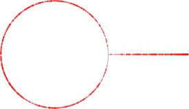
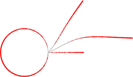
Figure 3: Left: the one-slit cluster of our process with 1,000 points in red sampled according to harmonic measure on the boundary. Right: the three-slit cluster of the process with 3,000 points sampled according to harmonic measure. Note in the second image that there are almost no points landing near the base of the most recent (longest) particle.

For $\eta>0$ the density $h_{n+1}$ in (2) is an exaggeration of harmonic measure, and in [17] the authors find that for $\eta>1$ the attachment distribution is concentrated around the point of highest harmonic measure, converging to a single atom as $\mathbf{c}\to 0$. For a slit particle the point of highest harmonic measure is the tip (see Figure 3), so this corresponds to the growth of a straight line.

In this paper, we find the equivalent phase transition in negative $\eta$: for $\eta<-2$ the attachment distribution is concentrated around the points of lowest harmonic measure. For a slit particle the two points of lowest harmonic measure are either side of the base (see Figure 3 again), and so $\theta_{2}\approx\theta_{1}\pm\beta$ with the probability of each tending to $1/2$ as $\mathbf{c}\to 0$. We go on to find that for all $n$ the distribution of $\theta_{n+1}$ is concentrated around $\theta_{n}\pm\beta$, and so the angle sequence approximates a random walk of step length $\beta\sim 2\mathbf{c}^{1/2}$.

This gives us the following statement about the driving function generating the cluster (see Section 1.4):

Proposition 5.

Fix some $T>0$. For $\eta<-2$ and if $\sigma(\mathbf{c})\leq\mathbf{c}^{2^{2^{1/\mathbf{c}}}}$ for all $\mathbf{c}<1$ let $(\theta_{n}^{\mathbf{c}})_{n\geq 1}$ be the sequence of angles we obtain from the $\mathrm{ALE}(0,\eta)$ process with capacity parameter $\mathbf{c}$. Let $\tau_{D}=\inf\{n\geq 2:\min_{\pm}|\theta_{n}-(\theta_{n-1}\pm\beta_{\mathbf{c}})|>D\}$, where $D=\mathbf{c}^{9/2}\sigma^{1/2}$. As $\mathbf{c}\to 0$,

$$\mathbb{P}\left[\tau_{D}\leq\left\lfloor T/\mathbf{c}\right\rfloor\right]=O(\mathbf{c}^{3}).$$

Let $\xi_{t}^{\mathbf{c}}=\theta_{\left\lfloor t/\mathbf{c}\right\rfloor+1}^{\mathbf{c}}$ for all $0\leq t\leq T$. Then

$$(\xi_{t}^{\mathbf{c}})_{t\in[0,T]}\to(2B_{t})_{t\in[0,T]}\text{ in distribution as }\mathbf{c}\to 0,$$

as a random variable in the Skorokhod space $D[0,T]$.

We explain in Section 1.4 that by using Loewner’s equation we can immediately turn a result about convergence of such a driving function into a result about convergence of clusters in an appropriate space $\mathcal{K}$. The main theorem of the paper therefore follows immediately from the proposition:

Theorem 6.

For $\eta,\sigma$ as in Proposition 5, let the corresponding $\mathrm{ALE}(0,\eta)$ cluster with $N=\left\lfloor T/\mathbf{c}\right\rfloor$ particles each of capacity $\mathbf{c}$ be $K_{N}^{\mathbf{c}}$. Then as $\mathbf{c}\to 0$, $K_{N}^{\mathbf{c}}$ converges in distribution as a random variable in $\mathcal{K}$ to a radial $\mathrm{SLE}_{4}$ curve of capacity $T$.

We can see in Figure 2 a cluster corresponding to a random walk, which despite being visibly composed of slits resembles an SLE₄ curve.

Remark.

We can give $\eta$ a physical interpretation if we think of growth in which access to environmental resources (proportional to harmonic measure) affects the growth rate in a non-linear manner. For negative $\eta$ we could also interpret ALE$(\alpha,\eta)$ as modelling a cluster in an environment which inhibits growth, so growth is concentrated in areas with the least exposure to the environment.

The most physically-relevant models are those with $\alpha=2$, where each particle in the cluster has approximately the same size. The case we consider, $\alpha=0$, is somewhat unphysical as the later particles have a macroscopic size (in our case the final particle has a shape approximating the whole path of the SLE₄). In our case the “visible” portion of each particle which is not hidden between other particles is microscopic, although the “visible” part of the later particles is still significantly longer than the first particles.

In any case, the remarkable thing about the $\eta<-2$, $\alpha=0$ case is that it is drawn from a family of models which naturally extend DLA-type growth, and we obtain an SLE₄ scaling-limit for a whole range of parameters. To this author’s knowledge no other conformal growth model in the plane has been rigorously proved to converge to a random limit such as the SLE.

Remark.

The convergence of attachment distributions to atomic measures for $\eta<-2$ complements the phase transition result of [17] in which it is shown that the limiting attachment measures are atomic for $\eta>1$. For $-2<\eta<1$ the distribution $h_{2}$ of the second particle is supported on all of $\mathbb{T}$ even in the limit $\mathbf{c}\to 0$, showing that we do indeed have three qualitative phases: for extreme values of $\eta$ the attachment measures are degenerate, but this is not the case for $-2<\eta<1$.

In Section 6 we conjecture that similar scaling results to Proposition 5 and Theorem 6 can be obtained with particles other than the slit. Using suitable particles which have a single point of contact with the circle, we believe that the limiting cluster is always an SLE_κ for some $\kappa\in[4,\infty]$ (where by SLE_∞ we mean a uniformly growing disc).

1.4 Loewner’s equation and the Schramm–Loewner evolution

We obtain a Schramm–Loewner evolution (SLE) cluster as the scaling limit of our model, so we will give a brief overview here of what SLE is and a few useful facts from Loewner theory which we use to establish our scaling limit. For a more detailed treatment, see [1], [8] and [3].

Firstly, we look at Loewner’s equation, which encodes our growing cluster by a “driving function” taking values on the circle.

Definition 7.

Let $\xi:[0,T]\to\mathbb{R}$ be a càdlàg function. Then there is a unique solution to Loewner’s equation

$$\varphi_{0}(z)=z,\quad\frac{\partial}{\partial t}\varphi_{t}(z)=\varphi_{t}^{\prime}(z)z\frac{z+e^{i\xi_{t}}}{z-e^{i\xi_{t}}},\quad z\in\Delta,$$ (4)

corresponding to a growing cluster via $\varphi_{t}(\Delta)=\mathbb{C}_{\infty}\setminus K_{t}$.

For a sequence of angles $(\theta_{n})_{n\geq 1}$ and a capacity $\mathbf{c}$, a growth model constructed as in Section 1.1 corresponds to the cluster obtained by solving Loewner’s equation with the driving function

$$\xi_{t}=\theta_{\left\lfloor t/\mathbf{c}\right\rfloor+1}.$$

Definition 8.

If $(B_{t})_{t\in[0,T]}$ is a standard Brownian motion, then the Schramm–Loewner evolution with parameter $\kappa>0$ (SLE_κ) is the random cluster obtained by solving Loewner’s equation with the driving function given by $\xi_{t}=\sqrt{\kappa}B_{t}$.

Remark.

One very useful property of Loewner’s equation for this paper is that the map $D[0,T]\to\mathcal{K}$ given by $\xi\mapsto K_{T}$ is continuous [7], where $D[0,T]$ is the usual Skorokhod space and $\mathcal{K}$ is the set of compact subsets of $\mathbb{C}$ containing $0$, equipped with the Carathéodory topology described in [3].

This property of Loewner’s equation means we can deduce convergence of an ALE(0,$\eta$) cluster to an SLE₄ for $\eta<-2$ by showing that the cluster corresponds to a driving function converging to $2B$ for a standard Brownian motion $B$ as $\mathbf{c}\to 0$.

Schramm–Loewner evolutions describe the scaling limits of many discrete models, such as the loop-erased random walk, which converges to an SLE₂ curve [9], or critical percolation, the boundaries of which has been related to SLE₆ [16]. SLEs have also been used to construct the quantum Loewner evolution (QLE) [13] family of clusters, which have been proposed as the scaling limits of the dielectric breakdown model on a number of random surfaces.

1.5 Structure of paper

Our proof of Proposition 5 will involve showing that the distribution of $\theta_{n+1}$ conditional on the previous angles $(\theta_{1},\dotsc,\theta_{n})$ converges to $\frac{1}{2}(\delta_{\theta_{n}+\beta}+\delta_{\theta_{n}-\beta})$, and so the whole path $\xi^{\mathbf{c}}$ converges to the same limit as a simple random walk with step length $\beta\sim 2\mathbf{c}^{1/2}$.

We can use a heuristic approach to see why we might expect this to be the case. If we formally take $\eta=-\infty$ and $\sigma=0$, so the $n$th attachment point $\theta_{n+1}$ is chosen uniformly from the finite set $\{\theta:\liminf_{\sigma\to 0}\inf_{w\in\mathbb{T}}|\Phi_{n}^{\prime}(e^{\sigma}e^{i\theta})|/|\Phi_{n}^{\prime}(e^{\sigma}w)|>0\}$ (i.e. among the “strongest poles” of $\Phi_{n}^{\prime}$), and let $\tau=\inf\{n:|\theta_{n}-\theta_{n-1}|\not=\beta\}$, then we can calculate that for $N=\left\lfloor T/\mathbf{c}\right\rfloor$ in the limit $\mathbf{c}\to 0$ we have $\mathbb{P}[\tau\leq N]\to 0$ as $\mathbf{c}\to 0$. In other words, at each step the distribution $h_{n+1}$ is equal to $\frac{1}{2}(\delta_{\theta_{n}-\beta}+\delta_{\theta_{n}+\beta})$.

Our approach for finite $\eta<-2$ will therefore be to find a small upper bound on $h_{n+1}(\theta)$ for $\theta$ away from the poles of $\Phi_{n}^{\prime}$ to deduce that $h_{n+1}$ is an approximation to a sum of atoms at the poles. Then we show separately that the contribution to $Z_{n}=\int_{\mathbb{T}}h_{n+1}(\theta)\,\mathrm{d}\theta$ from poles other than $e^{i(\theta_{n}\pm\beta)}$ is small.

In the actual model with $-\infty<\eta<-2$, we can only show that $h_{n+1}$ approximates $\frac{1}{2}(\delta_{\theta_{n}-\beta}+\delta_{\theta_{n}+\beta})$ as $\mathbf{c}\to 0$. However, weak convergence of these measures is not enough to prove Proposition 5, so we will need to introduce some extra notation to describe the possible behaviour of the process $(\theta_{n})_{n\geq 1}$, and make precise the way in which its steps converge to the SSRW steps as above.

Definition 9.

For a small $D=D(\mathbf{c})$ (which we will specify later), define the stopping time

$$\tau_{D}:=\inf\{n\geq 2:\min(|\theta_{n}-(\theta_{n-1}+\beta)|,|\theta_{n}-(\theta_{n-1}-\beta)|)>D\}.$$

Remark.

Given that $n<\tau_{D}$, we have a lot of information about the angle sequence $(\theta_{1},\dotsc,\theta_{n})$, and so can say quite a lot about the conditional distribution of $\theta_{n+1}$. In particular, we can say that the probability that $n+1=\tau_{D}$ is very low, and that the distribution of $\theta_{n+1}-\theta_{n}$ is (approximately) symmetric. The results of all the following sections will be used to establish these two facts.

Theorem 10.

Suppose that $\nu>2$. There exists a constant $A>0$ depending only on $\nu$ and $T$ such that when $\sigma\leq\mathbf{c}^{2^{2^{1/\mathbf{c}}}}$, then for $D=\mathbf{c}^{9/2}\sigma^{1/2}$, whenever $n<N\wedge\tau_{D}$ and $\mathbf{c}$ is sufficiently small,

$$\int_{F_{n}}h_{n+1}(\theta)\,\mathrm{d}\theta\leq A\mathbf{c}^{4}$$ (5)

with probability $1$, where $F_{n}=\{\theta\in\mathbb{T}:|\theta-(\theta_{n}+\beta)|\geq D\text{ and }|\theta-(\theta_{n}-\beta)|\geq D\}$, and with probability $1$

$$\left|\int_{\theta_{n}+\beta-D}^{\theta_{n}+\beta+D}h_{n+1}(\theta)\,\mathrm{d}\theta-\int_{\theta_{n}-\beta-D}^{\theta_{n}-\beta+D}h_{n+1}(\theta)\,\mathrm{d}\theta\right|\leq A\mathbf{c}^{11/4}.$$ (6)

In Section 2 we prove a number of technical results about the positions of the images and preimages of points $w\in\Delta$ under the maps $f_{j}$, $\Phi_{n}=f_{1}\circ\dotsb\circ f_{n}$, and $\Phi_{j,n}=\Phi_{j}^{-1}\circ\Phi_{n}$ when $w$ is close to the poles of $\Phi_{n}^{\prime}$. When dealing with points away from these poles, we make extensive use of results from [17]. Our estimates for the positions of these images will be useful when we find upper bounds on the derivative $|\Phi_{n}^{\prime}(w)|=|f_{n}^{\prime}(w)|\times|f_{n-1}^{\prime}(\Phi_{n-1,n}(w))|\times\dotsm\times|f_{1}^{\prime}(\Phi_{1,n}(w))|$, using lower bounds on the distance between $\Phi_{j,n}(w)$ and the poles of $f_{j}^{\prime}$.

In Section 3.1 we integrate the pre-normalised density $|\Phi_{n}^{\prime}(e^{\sigma+i\theta})|^{\nu}$ over the regions around $\theta_{n}\pm\beta$, and so obtain a lower bound on

$$Z_{n}=\int_{\mathbb{T}}|\Phi_{n}^{\prime}(e^{\sigma+i\theta})|^{\nu}\,\mathrm{d}\theta.$$

In Section 3.2 and Section 4 we find upper bounds on $|\Phi_{n}^{\prime}(e^{\sigma+i\theta})|$ for $\theta\in F_{n}$, and so using the lower bound on $Z_{n}$ we can establish the bound (5).

In Section 3.3 we establish the technical results needed to prove (6).

Remark.

In our proof of Theorem 10, the convergence of $h_{n+1}$ to $\frac{1}{2}(\delta_{\theta_{n}+\beta}+\delta_{\theta_{n}-\beta})$ does not rely on the convergence of $h_{1},\dotsc,h_{n}$ to these symmetric discrete measures, only that $n<\tau_{D}$. If we were to use the fact that the angle sequence up until time $n$ is very close to a simple symmetric random walk, then some properties (such as the fact that the longest interval on which a SSRW is monotone has length of order $O(\log n)$) would allow us to optimise our choice of $\sigma$ further than we have. However, for the convergence of our cluster to an SLE₄ curve, we do require a $\sigma$ which decays at least as quickly as $\mathbf{c}^{1/\mathbf{c}}$, which is already much faster than the fixed power of $\mathbf{c}$ used in [17] and elsewhere, so we have not attempted to optimise our choice of $\sigma\leq\mathbf{c}^{2^{2^{1/\mathbf{c}}}}$.

If $\sigma$ decays more slowly than $\mathbf{c}^{1/\mathbf{c}}$, but more quickly than $\mathbf{c}^{1/2}$, then heuristic arguments suggest that there is a period in which the driving function is a random walk, and then a period where the growth is measurable with respect to the random walk (i.e. a period of random growth and then a period of deterministic growth). We do not believe the resulting cluster converges to any known object as $\mathbf{c}\to 0$.

In Section 6 we define a family of particles for which we believe analogous versions of our main scaling result Theorem 6 holds. We conjecture that suitably constructed ALE($0,\eta$) models with $\eta<-2$ will converge to either an SLE_κ with $\kappa\geq 4$, or to a uniformly growing disc. We also believe that every $\kappa\geq 4$ is attained by this family.

1.6 Table of notation

As we introduce a lot of notation in this paper, we will give a list here so that it is possible to look up any notation appearing in any section without searching for where it was introduced.

Subsets of the complex plane

$\mathbb{C}_{\infty}$

The Riemann sphere, $\mathbb{C}\cup\{\infty\}$

$\mathbb{D}$

The open unit disc $\{z\in\mathbb{C}:|z|<1\}$.

$\overline{\mathbb{D}}$

The closed unit disc $\{z\in\mathbb{C}:|z|\leq 1\}$.

$\Delta$

The exterior disc $\mathbb{C}_{\infty}\setminus\overline{\mathbb{D}}$.

$\mathbb{T}$

The unit circle $\partial\Delta=\{z\in\mathbb{C}:|z|=1\}=\{e^{i\theta}:\theta\in\mathbb{R}\}$. We will often abuse notation and identify $\mathbb{T}$ with $\mathbb{R}/2\pi\mathbb{Z}$.

$\partial U$

The boundary of a set $U\subseteq\mathbb{C}_{\infty}$, defined as $\partial U=\overline{U}\setminus U^{\circ}$.

Conformal maps

$f$

The conformal map $f_{\mathbf{c}}\colon\Delta\to\Delta\setminus(1,1+d(\mathbf{c})]$ which we say attaches a particle to the unit circle at the point 1.

$f_{j}$

Given a sequence of angles $(\theta_{j})_{j\geq 1}$, $f_{j}$ attaches a particle to the unit circle at the point $e^{i\theta_{j}}$, so $f_{j}(z):=e^{i\theta_{j}}f(e^{-i\theta_{j}}z)$.

$\beta$

The distance from $1$ of the points which are sent to the base of the particle by $f$. Defined uniquely as the $\beta=\beta(\mathbf{c})\in(0,\pi)$ such that $f_{\mathbf{c}}(e^{\pm i\beta})=1$, and obeys $\beta\sim 2\mathbf{c}^{1/2}$ as $\mathbf{c}\to 0$.

$d$

The length of the particle attached by $f$, defined by $f_{\mathbf{c}}(1)=1+d(\mathbf{c})$. Obeys $d\sim\beta\sim 2\mathbf{c}^{1/2}$ as $\mathbf{c}\to 0$.

$\Phi_{n}$

The conformal map which attaches the entire cluster of $n$ particles to the unit circle at the point $1$. Constructed as $f_{1}\circ f_{2}\circ\dotsb\circ f_{n}$.

$\Phi_{j,n}$

The conformal map which attaches only the most recent $n-j$ particles to the unit circle. Given by $\Phi_{j,n}=\Phi_{j}^{-1}\circ\Phi_{n}$.

Model parameters

$\eta$

The parameter controlling the relationship between our attachment distributions and the harmonic measure on the boundary of the cluster. Throughout this paper we take $\eta<-2$.

$\nu$

We write $\nu=-\eta$. Note that $\nu>2$ throughout.

$T$

The total capacity of our cluster, fixed throughout.

$\mathbf{c}$

The capacity of each individual particle attached to the cluster. We consider in this paper the limit $\mathbf{c}\to 0$, so all the following parameters are functions of $\mathbf{c}$.

$\sigma$

A regularisation parameter, used so that we do not evaluate our conformal maps $\Phi_{n}^{\prime}$ at their poles on $\mathbb{T}$, instead evaluating everything on $e^{\sigma}\mathbb{T}$. We take $\sigma$ to be a function of $\mathbf{c}$, decaying very rapidly as $\mathbf{c}\to 0$: $\sigma\leq\mathbf{c}^{2^{2^{1/\mathbf{c}}}}$

$L$

The maximum distance of $z$ from $e^{i(\theta_{n}\pm\beta)}$ at which we rely on the estimates for $|\Phi_{j,n}(z)-e^{i\theta_{j+1}}|$ we obtain in the proof of Theorem 17. We take $L$ to be a function of $\mathbf{c}$ which does not decay as rapidly as $\sigma$: $L=\mathbf{c}^{2^{N+1}}$.

$D$

A bound on $\min_{\pm}|\theta_{n+1}-(\theta_{n}\pm\beta)|$ which holds with high probability. If this distance exceeds $D$, we stop the process. We can take $D=\mathbf{c}^{9/2}\sigma^{1/2}$.

Points in $\mathbb{T}$

$\theta^{\top}_{j}$

The point in $\mathbb{T}$ which $\theta_{j}$ was “supposed to” attach nearby to, i.e. the unique choice of $\theta_{j-1}\pm\beta$ which $\theta_{j}$ is within $D$ of (if $\theta_{j}$ is not within $D$ of either, we will have stopped the process at time $\tau_{D}\leq j$).

$\theta^{\bot}_{j}$

The choice of $\theta_{j-1}\pm\beta$ which isn’t $\theta_{j}^{\top}$.

$\widehat{z}^{n}_{j}$

The point on $\mathbb{T}$ corresponding to the base of the $j$th particle in the cluster $K_{n}$, for $1\leq j\leq n-1$. Given by $\widehat{z}^{n}_{j}:=\Phi_{j,n}^{-1}(e^{i\theta^{\bot}_{j+1}})$. See Figure 5 for an illustration. We refer to the points on $\mathbb{T}$ close to $\widehat{z}_{j}^{n}$ for some $j$ as singular points for $h_{n+1}$, and points away from all $\widehat{z}_{j}^{n}$ as regular points.

Probabilistic objects

$h_{n+1}$

The density of the distribution on $\mathbb{T}$ of $\theta_{n+1}$, conditional on $\theta_{1},\dotsc,\theta_{n}$. Given by $h_{n+1}(\theta)\propto|\Phi_{n}^{\prime}(e^{\sigma+i\theta})|^{\nu}$.

$Z_{n}$

The normalising factor for $h_{n+1}$. Given by $Z_{n}:=\int_{\mathbb{T}}|\Phi_{n}^{\prime}(e^{\sigma+i\theta})|^{\nu}\,\mathrm{d}\theta$.

$\mathbb{P}$

The law of $(\theta_{n})_{n\in\mathbb{N}}$. Implicitly depends on $\mathbf{c}$ and $\sigma$.

$\tau_{D}$

The first time at which some $\theta_{n+1}$ is further than $D$ from both of $\theta_{n}\pm\beta$. We stop the process when this happens, but show in Section 3 and Section 4 that with high probability $\tau_{D}>N:=\left\lfloor T/\mathbf{c}\right\rfloor$.

Approximations and bounds
We will use the following notation when we have two functions depending on a parameter $x$ which is converging to some $x_{0}\in\mathbb{R}\cup\{\pm\infty\}$, and we want to say the two functions are similar in some way, or that one bounds the other.

$f(x)\sim g(x)$

The ratio $\frac{f(x)}{g(x)}\to 1$ as $x\to x_{0}$.

$f(x)=O(g(x))$

The ratio $\left|\frac{f(x)}{g(x)}\right|$ is bounded above as $x\to x_{0}$, so there exists a constant $C>0$ such that $|f(x)|\leq C|g(x)|$ in a neighbourhood of $x_{0}$. The constant $C$ should not depend on any other parameter or variable. If the value of $C$ does depend on a parameter $\rho$, we will write $f(x)=O_{\rho}(g(x))$. Throughout this paper we hold $T$ and $\nu=-\eta$ fixed, so we may occasionally omit these as subscripts when the constant depends on them.

$f(x)=o(g(x))$

The ratio $\left|\frac{f(x)}{g(x)}\right|\to 0$ as $x\to x_{0}$.

When $f$ and $g$ are non-negative (particularly when they are probabilities or densities), we may use the following alternative notations.

$f(x)\lesssim g(x)$

The same as $f(x)=O(g(x))$, i.e. there exists a constant $C>0$ such that $f(x)\leq Cg(x)$ in a neighbourhood of $x_{0}$.

$f(x)\ll g(x)$

The same as $f(x)=o(g(x))$, i.e. $f(x)/g(x)\to 0$ as $x\to x_{0}$.

$f(x)\asymp g(x)$

Both $f(x)=O(g(x))$ and $g(x)=O(f(x))$, i.e. there exists constants $C_{1},C_{2}>0$ such that
$C_{1}g(x)\leq f(x)\leq C_{2}g(x)$ in a neighbourhood of $x_{0}$.

Finally, we may write $f(x)\approx g(x)$, but this will only be used informally to mean that $f$ and $g$ behave similarly in some sense.

2 Spatial distortion of points

There are several steps we need to establish our upper bound on $\int h_{n+1}(\theta)\,\mathrm{d}\theta$ in (5), including precise estimates for $|\Phi_{n}^{\prime}|$ near its poles. We can decompose the derivative

$$\Phi_{n}^{\prime}(w)=\prod_{j=0}^{n-1}f_{n-j}^{\prime}(\Phi_{n-j,n}(w))$$ (7)

where

$$\Phi_{k,n}:=\Phi_{k}^{-1}\circ\Phi_{n}=f_{k+1}\circ f_{k+2}\circ\dotsc\circ f_{n}.$$ (8)

Then we have precise estimates on $|f^{\prime}|$ near to its poles $e^{\pm i\beta}$, and upper bounds away from these poles, and so we write

$$|\Phi_{n}^{\prime}(w)|=\prod_{j=0}^{n-1}\left|f^{\prime}\left(e^{-i\theta_{n-j}}\Phi_{n-j,n}(w)\right)\right|.$$ (9)

We will show that if $w$ is close to one of $e^{i(\theta_{n}\pm\beta)}$, then for each $j$, the point $e^{-i\theta_{n-j}}\Phi_{n-j,n}(w)$ is close to a pole of $|f^{\prime}|$, and we will derive specific estimates on the distance in terms of the distance $|w-e^{i(\theta_{n}\pm\beta)}|$. Conversely, we will show that the only way for every image $e^{-i\theta_{n-j}}\Phi_{n-j,n}(w)$ to be close to a pole is for $w$ to be close to $e^{i(\theta_{n}\pm\beta)}$, and so the measure $\mathrm{d}h_{n+1}$ is concentrated around $\theta_{n}+\beta$ and $\theta_{n}-\beta$.

Firstly, we will establish an estimate for $|f^{\prime}|$ close to its poles $e^{\pm i\beta}$, and a universal upper bound away from these two points.

Lemma 11.

There are universal constants $A_{1},A_{2}>0$ such that for all $\mathbf{c}<1$, for $w\in\Delta$, if $|w-e^{i\beta}|\leq\frac{3}{4}\beta$, then

$$A_{1}\frac{\beta^{1/2}}{|w-e^{i\beta}|^{1/2}}\leq|f_{\mathbf{c}}^{\prime}(w)|\leq A_{2}\frac{\beta^{1/2}}{|w-e^{i\beta}|^{1/2}},$$ (10)

and similarly if $|w-e^{-i\beta}|\leq\frac{3}{4}\beta$.

Moreover, there is a third constant $A_{3}$ such that if $\min\{|w-e^{i\beta}|,|w-e^{-i\beta}|\}>\frac{3}{4}\beta$, then

$$|f_{\mathbf{c}}^{\prime}(w)|\leq A_{3}.$$

Proof.

See Lemma 5 of [17]. ∎

This lemma tells us that the derivative $|\Phi_{n}^{\prime}(w)|$ will be large only when many of the points $e^{-i\theta_{n-j}}\Phi_{n-j,n}(w)$ in (9) are close to one of the poles $e^{\pm i\beta}$. We will next introduce some technical estimates which will allow us to determine for which points $w$ this is true.

Remark.

If we imagine an idealised path in which $|\theta_{i+1}-\theta_{i}|=\beta$ for all $i$, then $f_{n}(e^{i(\theta_{n}\pm\beta)})=e^{i\theta_{n-1}}$, and $f_{n-1}(e^{i\theta_{n-1}})=e^{i\theta_{n-2}}$, and so on. Hence $\Phi_{n-j,n}(e^{i(\theta_{n}\pm\beta)})=e^{i\theta_{n-j+1}}=e^{i(\theta_{n-j}+s_{n-j}\beta)}$, where $s_{n-j}\in\{\pm 1\}$. So if a point $w$ is close to one of $e^{i(\theta_{n}\pm\beta)}$ then, as $f$ is continuous when extended to $\overline{\Delta}$, each of the points in (9) is close to $e^{is_{n-j}\beta}$, but continuity alone does not allow us to make precise what we mean by “$w$ is close to $e^{i(\theta_{n}\pm\beta)}$”, so to estimate the size of $|\Phi_{n}^{\prime}(w)|$, we need a precise estimate for $|f(w)-f(e^{i\beta})|$ in terms of $|w-e^{i\beta}|$.

Lemma 12.

For $w\in\Delta$, for all $\mathbf{c}<1$, if $|w-e^{i\beta}|\leq\beta/2$, then

$$|f_{\mathbf{c}}(w)-1|= 2(e^{\mathbf{c}}-1)^{1/4}|w-e^{i\beta}|^{1/2}$$ (11)

$$\times\left(1+O\left[\frac{|w-e^{i\beta}|}{\mathbf{c}^{1/2}}\vee\mathbf{c}^{1/4}|w-e^{i\beta}|^{1/2}\right]\right).$$

Proof.

We will work with the half-plane slit map $\widetilde{f}_{\mathbf{c}}\colon\mathbb{H}\to\mathbb{H}\setminus(0,i\sqrt{1-e^{-\mathbf{c}}}\,]$ by conjugating $f$ with the Möbius map $m_{\mathbb{H}}\colon\Delta\to\mathbb{H}$ given by

$$m_{\mathbb{H}}(w)=i\frac{w-1}{w+1},$$ (12)

and its inverse

$$m_{\Delta}(z):=m_{\mathbb{H}}^{-1}(z)=\frac{1-iz}{1+iz}.$$ (13)

The benefit of this is that $\widetilde{f}_{\mathbf{c}}$ has a simple explicit form:

$$\widetilde{f}_{\mathbf{c}}(\zeta)=e^{-\mathbf{c}/2}\sqrt{\zeta^{2}-(e^{\mathbf{c}}-1)}$$ (14)

where the branch of the square root is given by $\arg\colon\mathbb{C}\setminus[0,\infty)\to(0,2\pi)$, so we write

$$f_{\mathbf{c}}=m_{\Delta}\circ\widetilde{f}_{\mathbf{c}}\circ m_{\mathbb{H}}$$

and will derive a separate estimate for each of the three maps.

As $w$ is close to $e^{i\beta}=2e^{-\mathbf{c}}-1+2ie^{-\mathbf{c}}\sqrt{e^{\mathbf{c}}-1}$, we will expand each map about the images (given by a simple calculation) $m_{\mathbb{H}}(e^{i\beta})=-\sqrt{e^{\mathbf{c}}-1}$, $\widetilde{f}_{\mathbf{c}}(-\sqrt{e^{\mathbf{c}}-1})=0$, and $m_{\Delta}(0)=1$. Our calculations will show that $m_{\Delta}$ and $m_{\mathbb{H}}$ behave like scaling by a constant close to the relevant points, and that the behaviour of $f_{\mathbf{c}}$ seen in (11) is due to the behaviour of $\widetilde{f}_{\mathbf{c}}$ close to $\pm\sqrt{e^{\mathbf{c}}-1}$.

First, when $w=e^{i\beta}+\delta$,

$$|m_{\mathbb{H}}(w)-m_{\mathbb{H}}(e^{i\beta})| =\left|\frac{2\delta}{(e^{i\beta}+1+\delta)(e^{i\beta}+1)}\right|$$

$$=\frac{1}{2}e^{\mathbf{c}}|\delta|(1+O(|\delta|))$$ (15)

since a simple calculation shows that $|e^{i\beta}+1|^{2}=4e^{-\mathbf{c}}$.

Next, we will evaluate $\widetilde{f}_{\mathbf{c}}$ at a point close to one of the two preimages of $0$, $\pm\sqrt{e^{\mathbf{c}}-1}$:

$$\left|\widetilde{f}_{\mathbf{c}}(\pm\sqrt{e^{\mathbf{c}}-1}+\lambda)\right| =e^{-\mathbf{c}/2}\left|\sqrt{\pm 2\sqrt{e^{\mathbf{c}}-1}\lambda+\lambda^{2}}\right|$$

$$=\sqrt{2}e^{-\mathbf{c}/2}(e^{\mathbf{c}}-1)^{1/4}|\lambda|^{1/2}\left(1+O\left(\frac{|\lambda|}{\mathbf{c}^{1/2}}\right)\right).$$ (16)

Finally, for a small $z\in\mathbb{H}$,

$$|m_{\Delta}(z)-1|=\left|\frac{1-iz}{1+iz}-1\right|=\left|\frac{-2iz}{1+iz}\right|=2|z|(1+O(|z|)).$$ (17)

Then for $w$ close to $e^{i\beta}$, applying (15), (16) and (17) in turn, we obtain

$$|f(w)-1|=\ 2(e^{\mathbf{c}}-1)^{1/4}|w-e^{i\beta}|^{1/2}$$

$$\times \left(1+O\left(\frac{|w-e^{i\beta}|}{\mathbf{c}^{1/2}}\right)\right)\left(1+O\left(\mathbf{c}^{1/4}|w-e^{i\beta}|^{1/2}\right)\right).$$

Then for $\mathbf{c}^{3/2}\leq|w-e^{i\beta}|\leq\beta/2$, we have the estimate (11) with error term of order $\mathbf{c}^{-1/2}|w-e^{i\beta}|$, and for $|w-e^{i\beta}|\leq\mathbf{c}^{3/2}$ the error term has order $\mathbf{c}^{1/4}|w-e^{i\beta}|^{1/2}$. ∎

Remark.

Unlike most results in this section, we will not use the following lemma in Section 3, but it will be very useful in Section 4.2. We include it here and omit the proof as it is very similar to Lemma 12.

Lemma 13.

For all $\mathbf{c}<1$, if $z\in\Delta\setminus(1,1+d(\mathbf{c})]$ has $|z-1|\leq\mathbf{c}$, then

$$\min_{\pm}|f^{-1}(z)-e^{\pm i\beta}|=\frac{|z-1|^{2}}{4(e^{\mathbf{c}}-1)^{1/2}}\left(1+O\left(|z-1|\right)\right).$$

Now we have all the technical results we need in order to prove our lower bound on $|\Phi_{n}^{\prime}(w)|$ when $w$ is close to one of the two “most recent basepoints” $e^{i(\theta_{n}\pm\beta)}$. We will derive the bound itself in Section 3.1, and here we will show that each of the points $\Phi_{n-j,n}(w)$ in (9) is close to $e^{i\theta_{n-j+1}}$.

Proposition 14.

Let $L=L(\mathbf{c},N)=\mathbf{c}^{2^{N+1}}$, and let $n<N\wedge\tau_{D}$. If $\delta:=\min|w-e^{i(\theta_{n}\pm\beta)}|\leq 2L$, and $|w|\geq e^{\sigma}$, then for all $1\leq j\leq n$,

$$\left|\Phi_{n-j,n}(w)-e^{i\theta^{\top}_{n-j+1}}\right|=\left[2(e^{\mathbf{c}}-1)^{\frac{1}{4}}\right]^{2(1-2^{-j})}\delta^{2^{-j}}(1+O(\mathbf{c}^{4})).$$ (18)

Before we begin the proof we will introduce some notation in order to make the argument easier to follow.

Definition 15.

By definition of $\tau_{D}$, for each $n<\tau_{D}$ one of the two angles $\theta_{n-1}\pm\beta$ is within distance $D$ of $\theta_{n}$. We will call the closer of the two angles $\theta^{\top}_{n}$, and the other angle $\theta^{\bot}_{n}$.

Proof of Proposition 14.

We will proceed by induction on $j$. For $j=1$, the estimate (18) follows directly from Lemma 12. For a given $1\leq j\leq n-1$, assume that

$$|\Phi_{n-j,n}(w)-e^{i\theta^{\top}_{n-j+1}}|=\left[2(e^{\mathbf{c}}-1)^{\frac{1}{4}}\right]^{2(1-2^{-j})}\delta^{2^{-j}}(1+O(\mathbf{c}^{4})),$$

(as $|\theta_{n}-\theta^{\top}_{n}|<D\ll\mathbf{c}^{4}$, this certainly holds for $j=1$) and then by the triangle inequality, since $|e^{i\theta_{n-j}}-e^{i\theta^{\top}_{n-j}}|\leq|\theta_{n-j}-\theta^{\top}_{n-j}|<D$, we have

$$|\Phi_{n-j-1,n}(w)-e^{i\theta_{n-j}}|-D\leq| \Phi_{n-j-1,n}(w)-e^{i\theta^{\top}_{n-j}}|\leq|\Phi_{n-j-1,n}(w)-e^{i\theta_{n-j}}|+D.$$

Now by Lemma 12,

$$| \Phi_{n-j-1,n}(w)-e^{i\theta_{n-j}}|=|f_{n-j}(\Phi_{n-j,n}(w))-f_{n-j}(e^{i\theta^{\top}_{n-j+1}})|$$

$$=|f(e^{-i\theta^{\top}_{n-j+1}}\Phi_{n-j,n}(w))-1|$$

$$=2(e^{\mathbf{c}}-1)^{\frac{1}{4}}|e^{-i\theta^{\top}_{n-j+1}}\Phi_{n-j,n}(w)-1|^{1/2}(1+O(\mathbf{c}^{1/4}|e^{-i\theta^{\top}_{n-j+1}}\Phi_{n-j,n}(w)-1|^{1/2}))$$

$$=\left[2(e^{\mathbf{c}}-1)^{\frac{1}{4}}\right]^{1+(1-2^{-j})}\delta^{2^{-(j+1)}}(1+O(\mathbf{c}^{4}))(1+O(\mathbf{c}^{3/8}\delta^{2^{-(j+1)}}))$$

$$=\left[2(e^{\mathbf{c}}-1)^{\frac{1}{4}}\right]^{2(1-2^{-(j+1)})}\delta^{2^{-(j+1)}}(1+O(\mathbf{c}^{4}))$$

and the second error term is absorbed since $\delta^{2^{-(j+1)}}\leq(2L)^{2^{-(j+1)}}\leq\mathbf{c}^{4}$.

Now as $\delta=|w-e^{i(\theta_{n}\pm\beta)}|\geq|w|-1\geq\sigma$, and $D\sim\mathbf{c}^{9/2}\sigma^{1/2}$ (see Section 1.6), we have

$$|\Phi_{n-j-1,n}(w)-e^{i\theta^{\top}_{n-j}}| =|\Phi_{n-j-1,n}(w)-e^{i\theta_{n-j}}|\left(1+O\left(\frac{D}{\mathbf{c}^{\frac{1}{2}(1-2^{-(j+1)})}\delta^{2^{-(j+1)}}}\right)\right)$$

$$=|\Phi_{n-j-1,n}(w)-e^{i\theta_{n-j}}|\left(1+O\left(\mathbf{c}^{4}\sigma^{1/4}\right)\right),$$

and hence our result holds for all $1\leq j\leq n$ by induction. ∎

3 The newest basepoints

3.1 A lower bound on the normalising factor

We defined in (2) the density function $h_{n+1}(\theta)$ and the $n$th normalising factor

$$Z_{n}=\int_{\mathbb{T}}|\Phi_{n}^{\prime}(e^{\sigma+i\theta})|^{-\eta}\,\mathrm{d}\theta.$$ (19)

If we are going to find upper bounds on $h_{n+1}$ by bounding $|\Phi_{n}^{\prime}|$, then we will need to have some lower bound on the normalising factor $Z_{n}$. In this section, we will obtain a lower bound on $Z_{n}$, and it will give us our upper bound on $h_{n+1}$ in Section 4.2. First, we will need a good estimate for $|\Phi_{n}^{\prime}|$ around the main poles $e^{i(\theta_{n}\pm\beta)}$.

Lemma 16.

Let $n<\left\lfloor T/\mathbf{c}\right\rfloor\wedge\tau_{D}$. There are constants $A_{1},A_{2}>0$ such that for any $\mathbf{c}<1$, whenever $|\varphi|<L$,

$$A_{1}^{n}\frac{\mathbf{c}^{\frac{1}{2}(1-2^{-n})}}{(\sigma^{2}+\varphi^{2})^{\frac{1}{2}(1-2^{-n})}}\leq\left|\Phi_{n}^{\prime}\left(e^{\sigma+i(\theta_{n}\pm\beta+\varphi)}\right)\right|\leq A_{2}^{n}\frac{\mathbf{c}^{\frac{1}{2}(1-2^{-n})}}{(\sigma^{2}+\varphi^{2})^{\frac{1}{2}(1-2^{-n})}}$$

provided that $\sigma=\sigma(\mathbf{c})\leq L$.

Proof.

For $|\varphi|<L$, without loss of generality take $\theta=\theta_{n}+\beta+\varphi$. Since $\Phi_{n}=f_{1}\circ\dotsb\circ f_{n}$, by the chain rule,

$$|\Phi_{n}^{\prime}(e^{\sigma+i\theta})|=\prod_{j=0}^{n-1}\left|f^{\prime}\left(e^{-i\theta_{n-j}}\Phi_{n-j,n}(e^{\sigma+i\theta})\right)\right|,$$

where $\Phi_{k,n}=\Phi_{k}^{-1}\circ\Phi_{n}=f_{k+1}\circ f_{k+2}\circ\dotsb\circ f_{n}$.

By Proposition 14, if $\delta:=|e^{\sigma+i\theta}-e^{i(\theta_{n}+\beta)}|<2L$, then for all $1\leq j\leq n-1$, $|\Phi_{n-j,n}(e^{\sigma+i\theta})-e^{i\theta^{\top}_{n-j+1}}|=[2(e^{\mathbf{c}}-1)^{\frac{1}{4}}]^{2(1-2^{-j})}\delta^{2^{-j}}(1+O(\mathbf{c}^{4}))$, and so by Lemma 11 (the above estimate shows that $e^{-i\theta_{n-j}}\Phi_{n-j,n}(e^{\sigma+i\theta})$ is close enough to one of $e^{\pm i\beta}$ to apply this lemma),

$$\left|f^{\prime}\left(e^{-\theta_{n-j}}\Phi_{n-j,n}(e^{\sigma+i\theta})\right)\right| \asymp\beta^{1/2}|\Phi_{n-j,n}(e^{\sigma+i\theta})-e^{i\theta^{\top}_{n-j+1}}|^{-1/2}$$

$$=\beta^{1/2}[2(e^{\mathbf{c}}-1)^{\frac{1}{4}}]^{-(1-2^{-j})}\delta^{-2^{-j-1}}(1+O(\mathbf{c}^{4}))$$

$$\asymp\mathbf{c}^{2^{-(j+2)}}\delta^{-2^{-(j+1)}}.$$

For $j=0$, as $\Phi_{n,n}$ is the identity map,

$$|f^{\prime}(e^{-i\theta_{n}}\Phi_{n,n}(e^{\sigma+i\theta}))|=|f^{\prime}(e^{\sigma+i(\theta-\theta_{n})})| \asymp A_{1}\beta^{1/2}\delta^{-1/2}$$

$$\asymp A\mathbf{c}^{1/4}\delta^{-1/2}.$$

Now if we combine the bounds for each term in the above product for $|\Phi_{n}^{\prime}(e^{\sigma+i\theta})|$, we have

$$|\Phi_{n}^{\prime}(e^{\sigma+i\theta})| \geq\prod_{j=0}^{n-1}\left(A_{1}\mathbf{c}^{2^{-(j+2)}}\delta^{-2^{-(j+1)}}\right)$$

$$=A_{1}^{n}\mathbf{c}^{\frac{1}{2}(1-2^{-n})}\delta^{-(1-2^{-n})}.$$

and a similar upper bound. Finally, $\delta$ is given by

$$\delta =|e^{\sigma+i\theta}-e^{i(\theta_{n}+\beta)}|$$

$$=|e^{\sigma+i\varphi}-1|$$

$$\asymp(\sigma^{2}+\varphi^{2})^{1/2},$$

and so, modifying the constants as necessary, we have our result. ∎

We can now obtain our lower bound on the normalising factor.

Proposition 17.

If $\nu>2$, then there exists a constant $A$ depending only on $\nu$ such that for any fixed $T>0$, for sufficiently small $\mathbf{c}$ and for $n<\left\lfloor T/\mathbf{c}\right\rfloor\wedge\tau_{D}$,

$$Z_{n}\geq A^{n}\mathbf{c}^{\frac{\nu}{2}(1-2^{-n})}\sigma^{-[\nu(1-2^{-n})-1]}$$ (20)

provided that $\sigma=\sigma(\mathbf{c})\leq L$.

Proof.

The normalising factor $Z_{n}$ is given by the integral $\int_{\mathbb{T}}|\Phi_{n}^{\prime}(e^{\sigma+i\theta})|^{\nu}\,\mathrm{d}\theta$, and Lemma 16 gives us a lower bound on the integrand for $\theta$ close to $\theta_{n}+\beta$:

$$|\Phi_{n}^{\prime}(e^{\sigma+i(\theta_{n}+\beta+\varphi)})|^{\nu}\geq A^{n}\mathbf{c}^{\frac{\nu}{2}(1-2^{-n})}(\sigma^{2}+\varphi^{2})^{-\frac{\nu}{2}(1-2^{-n})}$$

when $|\varphi|<L$.

We will now integrate our lower bound over the interval $(\theta_{n}+\beta-L,\theta_{n}+\beta+L)$. First, note that

$$\int_{-L}^{L}(\sigma^{2}+\varphi^{2})^{-\frac{\nu}{2}(1-2^{-n})}\,\mathrm{d}\varphi =\int_{-L/\sigma}^{L/\sigma}(\sigma^{2}+\sigma^{2}x^{2})^{-\frac{\nu}{2}(1-2^{-n})}\,\sigma\mathrm{d}x$$

$$=\sigma^{1-\nu(1-2^{-n})}\int_{-L/\sigma}^{L/\sigma}\frac{\mathrm{d}x}{(1+x^{2})^{\frac{\nu}{2}(1-2^{-n})}}$$

$$\geq A^{\prime}\sigma^{1-\nu(1-2^{-n})}$$

for a constant $A^{\prime}$, since the integral term on the right hand side is increasing as $\mathbf{c}\to 0$ because $\sigma\ll L$. Note that this all remains true for any $\eta<0$, and the fact that $\eta<-2$ will only be necessary in Section 3.2.

Finally, we can put together our bounds (and modify our constant $A$) to get

$$\int_{\theta_{n}+\beta-L}^{\theta_{n}+\beta+L}|\Phi_{n}^{\prime}(e^{\sigma+i\theta})|^{\nu}\,\mathrm{d}\theta \geq A^{n}\mathbf{c}^{\frac{\nu}{2}(1-2^{-n})}\int_{-L}^{L}(\sigma^{2}+\varphi^{2})^{-\frac{\nu}{2}(1-2^{-n})}\,\mathrm{d}\varphi$$

$$\geq A^{n}\mathbf{c}^{\frac{\nu}{2}(1-2^{-n})}\sigma^{1-\nu(1-2^{-n})}$$

as required. ∎

3.2 Concentration about each basepoint

Most of our upper bounds on $|\Phi_{n}^{\prime}|$ will be established in Section 4, but we will find one here as it uses the estimates from the previous section. Using the terminology we introduce in Section 4 and illustrate in Figure 4, in this section we look at singular points which are within $L$ of one of the “main” poles $e^{i(\theta_{n}\pm\beta)}$ so the estimate of Lemma 16 is valid, but are not within $D$ of these poles.

Proposition 18.

Let $n<\left\lfloor T/\mathbf{c}\right\rfloor\wedge\tau_{D}$. For $\sigma(\mathbf{c})\leq\mathbf{c}^{2^{2^{1/\mathbf{c}}}}$, then with $L=\mathbf{c}^{2^{N+1}}$ and $D=\mathbf{c}^{9/2}\sigma^{1/2}\ll L$,

$$\frac{1}{Z_{n}}\int_{[-L,L]\setminus[-D,D]}|\Phi_{n}^{\prime}(e^{\sigma+i(\theta_{n}\pm\beta+\varphi)})|^{\nu}\,\mathrm{d}\varphi=o(\mathbf{c}^{\gamma})$$

as $\mathbf{c}\to 0$, for any constant $\gamma>0$.

Proof.

Using the symmetry of our upper bound in Lemma 16, it will be enough to find the upper bound $\int_{D}^{L}|\Phi_{n}^{\prime}(e^{\sigma+i(\theta_{n}+\beta+\varphi)})|^{\nu}\,\mathrm{d}\varphi\ll\mathbf{c}^{\gamma}Z_{n}$. We have, modifying the constant $A_{2}$ where necessary,

$$\int_{D}^{L}|\Phi_{n}^{\prime}(e^{\sigma+i(\theta_{n}+\beta+\varphi)})|^{\nu}\,\mathrm{d}\varphi \leq A_{2}^{n}\mathbf{c}^{\frac{\nu}{2}(1-2^{-n})}\int_{D}^{L}(\sigma^{2}+\varphi^{2})^{-\frac{\nu}{2}(1-2^{-n})}\,\mathrm{d}\varphi$$

$$=A_{2}^{n}\frac{\mathbf{c}^{\frac{\nu}{2}(1-2^{-n})}}{\sigma^{\nu(1-2^{-n})-1}}\int_{D/\sigma}^{L/\sigma}(1+x^{2})^{-\frac{\nu}{2}(1-2^{-n})}\,\mathrm{d}x$$

$$\leq A_{2}^{n}\frac{\mathbf{c}^{\frac{\nu}{2}(1-2^{-n})}}{\sigma^{\nu(1-2^{-n})-1}}\int_{D/\sigma}^{L/\sigma}x^{-\nu(1-2^{-n})}\,\mathrm{d}x$$

$$\leq A_{2}^{n}\frac{\mathbf{c}^{\frac{\nu}{2}(1-2^{-n})}}{D^{\nu(1-2^{-n})-1}},$$

and so, using our lower bound on $Z_{n}$,

$$\frac{\int_{D}^{L}|\Phi_{n}^{\prime}(e^{\sigma+i(\theta_{n}+\beta+\varphi)})|^{\nu}\,\mathrm{d}\varphi}{Z_{n}} \leq(A_{2}/A)^{n}\left(\frac{\sigma}{D}\right)^{\nu(1-2^{-n})-1}$$

$$=(A_{2}/A)^{n}\left(\mathbf{c}^{-9/2}\sigma^{1/2}\right)^{\nu(1-2^{-n})-1}$$

which, since $\nu(1-2^{-n})-1\geq\frac{1}{2}\nu-1>0$, decays faster than any power of $\mathbf{c}$ as $\mathbf{c}\to 0$. ∎

Note that the above proof is the only place in which we use that $\eta<-2$. If $-2\leq\eta<0$, then $h_{2}$ achieves its maximum around the two bases of the first particle, but does not have strong concentration around these points. For $-2<\eta<0$ $h_{2}$ is still supported on all of $\mathbb{T}$ as $\mathbf{c}\to 0$, so there is no concentration. If $\eta=-2$, $h_{2}$ is supported only nearby to $\theta_{1}\pm\beta$, but the event $D<|\theta_{2}-(\theta_{1}\pm\beta)|\ll\beta$ retains a high probability as $\mathbf{c}\to 0$. On this event, $\theta_{2}$ is not close enough to $\theta_{1}\pm\beta$ for our inductive arguments in Proposition 14 and Lemma 16 to apply. We can no longer guarantee that the poles of the second particle are stronger than the older pole at the base of the first particle, and so lose the SSRW-like behaviour of $(\theta_{n})_{n\geq 1}$. It then becomes extremely difficult to say how the process behaves, but the scaling limit as $\mathbf{c}\to 0$ is unlikely to be described by the Schramm–Loewner evolution.

3.3 Symmetry of the two most recent basepoints

There are two parts to the statement in Theorem 10 about convergence of $h_{n+1}$ to the discrete measure $\frac{1}{2}(\delta_{\theta_{n}-\beta}+\delta_{\theta_{n}+\beta})$: the previous two sections and Section 4 establish that $h_{n+1}$ is concentrated very tightly around $\theta_{n}\pm\beta$, and we will show here that the weight given to each of these two points is approximately equal.

Remark.

Unlike the results from the previous two sections, the following proposition is not inductive, i.e. as long as $n<\left\lfloor T/\mathbf{c}\right\rfloor\wedge\tau_{D}$, the density $h_{n+1}$ is approximately symmetric, even if the choices of the previous angles were not made symmetrically. Even in the extreme case where $(\theta_{n})_{n\in\mathbb{N}}$ is close to an arithmetic progression: $\theta_{2}\approx\theta_{1}+\beta$, $\theta_{3}\approx\theta_{2}+\beta,\dotsc,\theta_{n}\approx\theta_{n-1}+\beta$, we still have an almost symmetric $h_{n+1}$.

Proposition 19.

Let $n<\left\lfloor T/\mathbf{c}\right\rfloor\wedge\tau_{D}$. Then

$$\sup_{|\varphi|<D}\left|\log\left(\frac{\left|\Phi_{n}^{\prime}\left(e^{\sigma+i(\theta_{n}+\beta+\varphi)}\right)\right|}{\left|\Phi_{n}^{\prime}\left(e^{\sigma+i(\theta_{n}-\beta-\varphi)}\right)\right|}\right)\right|\leq A\mathbf{c}^{11/4}$$

for some constant $A$ depending only on $T$.

Proof.

Let $z_{\pm}=\exp\left(\sigma+i\left[\theta_{n}\pm(\beta+\varphi)\right]\right)$ for $|\varphi|<D$, and write $\lambda_{\pm}=z_{\pm}-e^{i(\theta_{n}\pm\beta)}$. We can then write

$$\log\left(\frac{|\Phi_{n}^{\prime}(z_{+})|}{|\Phi_{n}^{\prime}(z_{-})|}\right)=\sum_{j=0}^{n-1}\log\left(\frac{|f_{n-j}^{\prime}(\Phi_{n-j,n}(z_{+}))|}{|f_{n-j}^{\prime}(\Phi_{n-j,n}(z_{-}))|}\right)$$ (21)

and so we can estimate each term in (21) separately.

The $j=0$ term is exactly 0, by the symmetry of $|f_{n}^{\prime}|$ about $\theta_{n}$.

For $1\leq j\leq n-1$, we will use Lemma 4 of [17], which states that $f^{\prime}(z)=\frac{f(z)}{z}\frac{z-1}{(z-e^{i\beta})^{1/2}(z-e^{-i\beta})^{1/2}}$, to compare the two derivatives in the $j$th term of (21). Write $z_{\pm}^{j}=\Phi_{n-j,n}(z_{\pm})$, then the $j$th term in (21) is

$$|f_{n-j}^{\prime}(z_{\pm}^{j})|=\frac{|z_{\pm}^{j+1}|}{|z_{\pm}^{j}|}\frac{|z_{\pm}^{j}-e^{i\theta_{n-j}}|}{|z_{\pm}^{j}-e^{i\theta^{\bot}_{n-j+1}}|^{1/2}|z_{\pm}^{j}-e^{i\theta^{\top}_{n-j+1}}|^{1/2}}$$ (22)

There will be some telescoping in the product which allows us to find

$$\prod_{j=1}^{n-1}\frac{|z_{\pm}^{j+1}|}{|z_{\pm}^{j}|}=\frac{|z_{\pm}^{n}|}{|z_{\pm}^{1}|}.$$

Then recall that in Section 2 we derived estimates for the distance of $z_{\pm}^{n}$ from $e^{i\theta^{\top}_{n-j+1}}$ in terms of $|\lambda_{\pm}|$. So by Proposition 14, as $e^{i\theta^{\top}_{1}}=1$,

$$|z_{\pm}^{n}-1|=\left[2(e^{\mathbf{c}}-1)^{\frac{1}{4}}\right]^{2(1-2^{-n})}|\lambda_{\pm}|^{2^{-n}}(1+O(\mathbf{c}^{4}))=O(\mathbf{c}^{17/4})$$

since $|\lambda_{\pm}|^{2^{-n}}\lesssim D^{2^{-n}}\ll L^{2^{-n}}\leq\mathbf{c}^{4}$. Therefore $|z_{\pm}^{n}|=1+O(\mathbf{c}^{17/4})$, and similarly $|z_{\pm}^{1}|=1+O(\mathbf{c}^{17/4})$.

Having dealt with the first fraction in all derivatives (22) at once, we will tackle the remaining terms individually for each $1\leq j\leq n-1$.

First note that by definition of $\theta^{\top}_{n-j+1}$, $|e^{i\theta^{\top}_{n-j+1}}-e^{i\theta_{n-j}}|=|e^{i\beta}-1|$. Hence, using Proposition 14 again,

$$|z_{\pm}^{j}-e^{i\theta_{n-j}}| =|e^{i\theta^{\top}_{n-j+1}}-e^{i\theta_{n-j}}|\left[1+O\left(\frac{|z_{\pm}^{j}-e^{i\theta^{\top}_{n-j+1}}|}{|e^{i\theta^{\top}_{n-j+1}}-e^{i\theta_{n-j}}|}\right)\right]$$

$$=|e^{i\beta}-1|\left[1+O\left(\mathbf{c}^{-2^{-(j+1)}}|\lambda_{\pm}|^{2^{-j}}\right)\right]$$

$$=|e^{i\beta}-1|\left[1+O\left(\mathbf{c}^{15/4}\right)\right]$$

since $|\lambda_{\pm}|^{2^{-j}}\ll L^{2^{-(n-1)}}\leq\mathbf{c}^{4}$.

Similarly,

$$|z_{\pm}^{j}-e^{i\theta^{\bot}_{n-j+1}}| =|e^{2i\beta}-1|(1+O(\mathbf{c}^{15/4})),$$

and finally, directly from Proposition 14,

$$|z_{\pm}^{j}-e^{i\theta^{\top}_{n-j+1}}|=\left[2(e^{\mathbf{c}}-1)^{\frac{1}{4}}\right]^{2(1-2^{-j})}|\lambda_{\pm}|^{2^{-j}}(1+O(\mathbf{c}^{4})).$$

Note that for the three estimates we just found, the only part which depends on the choice of $\pm$ is the error term (as $|\lambda_{+}|=|\lambda_{-}|$). Hence the part of the ratio of $|f_{n-j}^{\prime}(z_{+}^{j})|$ to $|f_{n-j}^{\prime}(z_{-}^{j})|$ which comes from the second fraction in (22) is just $1+O(\mathbf{c}^{15/4})$.

We can therefore find a constant $A$ (which does not depend on $n$ or $\varphi$) such that for each $1\leq j\leq n-1$, $\left|\log\left(\frac{|f_{n-j}^{\prime}(z_{+}^{j})|}{|f_{n-j}^{\prime}(z_{-}^{j})|}\right)\right|\leq A\mathbf{c}^{15/4}$. As there are $O_{T}(\mathbf{c}^{-1})$ such terms in the product (21), we have

$$\left|\log\left(\frac{|\Phi_{n}^{\prime}(z_{+})|}{|\Phi_{n}^{\prime}(z_{-})|}\right)\right|=O_{T}(\mathbf{c}^{11/4})$$

as claimed. ∎

Now we can deduce that $h_{n+1}$ gives (asymptotically) the same measure to the sets $(\theta_{n}+\beta-D,\theta_{n}+\beta+D)$ and $(\theta_{n}-\beta-D,\theta_{n}-\beta+D)$.

Remark.

Recall that earlier we used the heuristic argument that if $\eta=-\infty$ (so we choose from points with the highest-order pole), then we attach the $(n+1)$th particle to one of $\theta_{n}\pm\beta$, with equal probability. With finite $\eta<-2$, the derivative $|\Phi_{n}^{\prime}|$ in fact differs slightly at each of $e^{\sigma+i(\theta_{n}+\beta)}$ and $e^{\sigma+i(\theta_{n}-\beta)}$, and so choosing to attach a particle at $e^{i\theta}$ for $\theta$ maximising $|\Phi_{n}^{\prime}(e^{\sigma+i\theta})|$ leads to a deterministic process after the second step rather than our SLE₄ limit.

However, when we have a finite $\eta<-2$, integrating over the range $(-D,D)$ around each $\theta_{n}\pm\beta$ means that only the asymptotic behaviour of $|\Phi_{n}^{\prime}|$ needs to be the same to guarantee symmetry between the two points $\theta_{n}\pm\beta$.

Corollary 20.

For $n<\left\lfloor T/\mathbf{c}\right\rfloor\wedge\tau_{D}$,

$$\left|\int_{-D}^{D}h_{n+1}(\theta_{n}+\beta+\varphi)\,\mathrm{d}\varphi-\int_{-D}^{D}h_{n+1}(\theta_{n}-\beta-\varphi)\,\mathrm{d}\varphi\right|=O_{T}(\mathbf{c}^{11/4}).$$ (23)

Proof.

From Proposition 19, we have

$$\int_{-D}^{D} h_{n+1}(\theta_{n}+\beta+\varphi)\,\mathrm{d}\varphi-\int_{-D}^{D}h_{n+1}(\theta_{n}-\beta-\varphi)\,\mathrm{d}\varphi$$

$$=\frac{1}{Z_{n}}\int_{-D}^{D}\left(|\Phi_{n}^{\prime}(e^{\sigma+i(\theta_{n}+\beta+\varphi)})|^{\nu}-|\Phi_{n}^{\prime}(e^{\sigma+i(\theta_{n}-\beta-\varphi)})|^{\nu}\right)\mathrm{d}\varphi$$

$$=\frac{1}{Z_{n}}\int_{-D}^{D}\left(|\Phi_{n}^{\prime}(e^{\sigma+i(\theta_{n}+\beta+\varphi)})|^{\nu}-e^{O_{T}(\mathbf{c}^{11/4})}|\Phi_{n}^{\prime}(e^{\sigma+i(\theta_{n}+\beta+\varphi)})|^{\nu}\right)\mathrm{d}\varphi$$

$$=O_{T}\left(\mathbf{c}^{11/4}\frac{\int_{-D}^{D}|\Phi_{n}^{\prime}(e^{\sigma+i(\theta_{n}+\beta+\varphi)})|^{\nu}\,\mathrm{d}\varphi}{Z_{n}}\right)$$

which is just $O_{T}(\mathbf{c}^{11/4})$ by definition of $Z_{n}$. ∎

4 Analysis of the density away from the main basepoints

In this section, we will classify the points $\theta\in\mathbb{T}$ with $|\theta-(\theta_{n}\pm\beta)|\geq D$ (i.e. the set $F_{n}$ from Theorem 10) into regular points $R_{n}$ where $h_{n+1}(\theta)\ll 1$, and singular points $S_{n}$ where $h_{n+1}(\theta)\gtrsim 1$. We make this classification based on how close the image $\Phi_{n}(e^{\sigma+i\theta})$ is to the common basepoint of the cluster, which is the image of all the poles of $\Phi_{n}^{\prime}$, as we can see in Figure 4.

In Section 4.1 we make this classification explicit and establish a bound on $h_{n+1}$ for the regular points. In Section 4.2 we analyse the singular points more carefully and establish an upper bound on $\int_{S_{n}}h_{n+1}(\theta)\,\mathrm{d}\theta$ using similar techniques as in Section 3.1.

Figure 4: We can see on the left the three types of points in $e^{\sigma}\mathbb{T}$ for the three-slit cluster: we have the singular points in red and yellow and the regular points in grey dots. The right hand side of the diagram shows that a point on $e^{\sigma}\mathbb{T}$ is classified as regular if its image under $\Phi_{n}$ is far from the common basepoint (Proposition 21 in Section 4.1 shows that this implies $h_{n+1}\ll 1$), and the singular points are further classified into the two main (red) arcs containing $e^{i(\theta_{n}\pm\beta)}$, and the other (yellow) singular points. We have $h_{n+1}\gtrsim 1$ for all singular points, but we obtained a lower bound on the integral of $|\Phi_{n}^{\prime}|$ over the red regions in Section 3.1, and we will find an upper bound on the integral of this derivative over the yellow regions in Section 4.2. Note that the choice of $\sigma$ we have used for this diagram is around $\mathbf{c}^{2}$ rather than the much smaller $\mathbf{c}^{2^{1/\mathbf{c}}}$, which is necessary to make the envelope $\Phi_{3}(e^{\sigma}\mathbb{T})$ clear, but does mean that some “regular” points are closer to the common basepoints than the red “singular” points. With a sufficiently small $\sigma$ this isn’t the case.

4.1 Regular points

In this section, we will establish a criterion for $\theta\in\mathbb{T}$ to be in our set of regular points for which $h_{n+1}(\theta)\ll 1$, based on the position of $\Phi_{n}(e^{\sigma+i\theta})$, as shown in Figure 4.

We will first derive an upper bound on $|\Phi_{n}^{\prime}(w)|$ in terms of $|\Phi_{n}(w)-1|$, so we can classify $w\in\Delta$ as a regular point using the distance of its image $\Phi_{n}(w)$ from $1$.

Proposition 21.

Let $n<N(\mathbf{c})\wedge\tau_{D}$. For $\theta\in\mathbb{R}$, let $w=\exp(\sigma+i\theta)$.

For any function $a:\mathbb{R}_{+}\to\mathbb{R}_{+}$ with $D^{2^{-N}}/\beta\leq a(\mathbf{c})\leq\mathbf{c}^{3/2}$ for all $0<\mathbf{c}<1$, if

$$|\Phi_{n}(w)-1|\geq\beta a(\mathbf{c})$$ (24)

then, for sufficiently small $\mathbf{c}$,

$$|\Phi_{n}^{\prime}(w)|\leq A^{n}\beta^{n/2}\left(\frac{a(\mathbf{c})}{8}\right)^{-\frac{1}{2}(2^{n}-1)}$$ (25)

where $A$ is a universal constant independent of $a$.

Proof.

We will use the estimate (11) from Lemma 12. For convenience, let $z=\Phi_{n}(w)$, and we will estimate $|\Phi_{n}^{\prime}(w)|=|(\Phi_{n}^{-1})^{\prime}(z)|^{-1}$ by using (9) and estimating each term separately, using Lemma 12 to obtain estimates on $\Phi_{n-j,n}(w)=\Phi_{n-j}^{-1}(z)$ by induction on $j$.

First we claim that for $A(\mathbf{c})\leq\mathbf{c}^{1/2}$, and $\zeta\in\Delta\setminus(1,1+d(\mathbf{c})]$, if we have $|\zeta-1|\geq\beta A(\mathbf{c})$, then

$$\min_{\pm}(|f^{-1}(\zeta)-e^{\pm i\beta}|)\geq\frac{1}{4}\beta A(\mathbf{c})^{2}$$ (26)

for all $\mathbf{c}<c_{0}$, where $c_{0}>0$ is a universal constant which doesn’t depend on $A$.

To see this, suppose that $|f^{-1}(\zeta)-e^{i\beta}|<\frac{1}{4}\beta A(\mathbf{c})^{2}$. Then by Lemma 12, setting $\varepsilon=2^{1/4}-1>0$, for sufficiently small $\mathbf{c}$,

$$|\zeta-1| =|f(f^{-1}(\zeta))-f(e^{i\beta})|$$

$$=2(e^{\mathbf{c}}-1)^{1/4}|f^{-1}(\zeta)-e^{i\beta}|^{1/2}(1+O\left(A(\mathbf{c})^{2}\vee\mathbf{c}^{1/2}A(\mathbf{c})\right))$$

$$<2(\beta/2)^{1/2}(1+\varepsilon)\frac{1}{2}\beta^{1/2}A(\mathbf{c})(1+\varepsilon)$$

$$=\beta A(\mathbf{c}),$$

so we have shown the contrapositive for our claim.

The derivative $|\Phi_{n}^{\prime}(w)|$ is decomposed in (9) into the product of $n$ terms $\left|f^{\prime}(e^{-i\theta_{k}}\Phi_{k,n}(w))\right|$, and so we can find an upper bound on $|\Phi_{n}^{\prime}(w)|$ by obtaining lower bounds on each $|\Phi_{k,n}(w)-e^{i(\theta_{k}\pm\beta)}|=|\Phi_{k}^{-1}(z)-e^{i(\theta_{k}\pm\beta)}|$ for $0\leq k\leq n-1$ and applying Lemma 11.

We claim that, for each $0\leq k\leq n-1$,

$$|\Phi_{k}^{-1}(z)-e^{i\theta_{k+1}}|\geq\beta\times 8\left(\frac{a(\mathbf{c})}{8}\right)^{2^{k}}$$ (27)

and we will show this using induction. For $k=0$, (27) is exactly the assumption (24) of this proposition. For $k\geq 1$, we assume as the induction step that

$$|\Phi_{k-1}^{-1}(z)-e^{i\theta_{k}}|\geq\beta\times 8\left(\frac{a(\mathbf{c})}{8}\right)^{2^{k-1}}$$

and aim to obtain (27) by applying (26).

Taking $A(\mathbf{c})=8\left(\frac{a(\mathbf{c})}{8}\right)^{2^{k-1}}$ in (26) gives us

$$|\Phi_{k}^{-1}(z)-e^{i\theta^{\top}_{k+1}}|\geq\beta\times 16\left(\frac{a(\mathbf{c})}{8}\right)^{2^{k}},$$

and so since $8\beta\left(\frac{a(\mathbf{c})}{8}\right)^{2^{k}}\geq 2D$ when $k\leq N\wedge\tau_{D}$ (for $\mathbf{c}$ sufficiently small),

$$|\Phi_{k}^{-1}(z)-e^{i\theta_{k+1}}| \geq|\Phi_{k}^{-1}(z)-e^{i\theta^{\top}_{k+1}}|-|e^{i\theta_{k+1}}-e^{i\theta^{\top}_{k+1}}|$$

$$\geq 16\beta\left(\frac{a(\mathbf{c})}{8}\right)^{2^{k}}-2D$$

$$\geq 8\beta\left(\frac{a(\mathbf{c})}{8}\right)^{2^{k}},$$

verifying (27).

Then (27) tells us, using (26), that for each $0\leq k\leq n-1$,

$$|\Phi_{k}^{-1}(z)-e^{i(\theta_{k}\pm\beta)}|\geq\beta\times 16\left(\frac{a(\mathbf{c})}{8}\right)^{2^{k}},$$ (28)

and so, by Lemma 11, for $\mathbf{c}$ sufficiently small,

$$|\Phi_{n}^{\prime}(w)| =\prod_{k=0}^{n-1}|f_{k+1}^{\prime}(\Phi_{k}^{-1}(z))|$$

$$\leq A^{n}\beta^{n/2}\prod_{k=1}^{n-1}\left(\beta^{1/2}\left[\beta\times 16\left(\frac{a(\mathbf{c})}{8}\right)^{2^{k}}\right]^{-1/2}\right)$$

$$=(A/4)^{n}\beta^{n/2}\left(\frac{a(\mathbf{c})}{8}\right)^{-\frac{1}{2}(2^{n}-1)}$$

for a universal constant $A$. ∎

In the next section we will use these results with $a(\mathbf{c})$ equal to $\frac{L}{4\beta}$. We can easily check now that if we use this choice of $a$ in Proposition 21 then, comparing (25) with (20), if $\sigma$ decays as fast as $\mathbf{c}^{2^{2^{N}}}$ then $|\Phi_{n}^{\prime}(z)|^{\nu}$ is far smaller than $\mathbf{c}Z_{n}$, for $z$ away from the preimages of $e^{i\theta_{1}}$, and so if we classify our regular points as those $\theta$ for which $|\Phi_{n}(e^{\sigma+i\theta})-1|\geq L/4$ then we do have $\sup\limits_{\theta\in R_{n}}h_{n+1}(\theta)\ll 1$.

4.2 Old singular points

In Section 3, we established a lower bound on the $n$th normalising factor $Z_{n}$. So to show that the probability is low that the $(n+1)$th particle is attached at a point in $E\subseteq\mathbb{T}$, we need to find an upper bound on $\int_{E}|\Phi_{n}^{\prime}(e^{\sigma+i\theta})|^{\nu}\,\mathrm{d}\theta$.

We did this over certain regions in Section 4.1 by finding a bound $|\Phi_{n}^{\prime}(e^{\sigma+i\theta})|^{\nu}\ll\mathbf{c}Z_{n}$. In this section we will consider singular points where we can have $|\Phi_{n}^{\prime}(e^{\sigma+i\theta})|^{\nu}\gg Z_{n}$. However, if we look at Figure 4 we can see that not all singular points are close to the preimages $\theta_{n}\pm\beta$ of the base of the most recent particle; there are singular points at the preimages of the base of each particle. We will therefore need to estimate the integrand $|\Phi_{n}^{\prime}|^{\nu}$ more carefully, and show that when integrated over the singular points around these old bases and normalised by $Z_{n}$, the resulting probability is small.

The first thing we need to do is to describe precisely which points we are integrating over. We have previously classified our points into regular points $R_{n}$ and singular points $S_{n}$ by looking at the distance $|\Phi_{n}(w)-1|$. Points are singular when $|\Phi_{n}(w)-1|<\beta a(\mathbf{c})$ (for an $a(\mathbf{c})$ we will specify later), and we will find a way of differentiating between the “new” singular points around the preimages of the $n$th particle’s base and the “older” singular points around the preimages of the other particles’ bases. To make this clear, we will first give names to all of these preimages.

Figure 5: The construction of a cluster with three particles by composing the three maps $f_{3}$, $f_{2}$ and $f_{1}$. The top left diagram has labelled the four poles $\widehat{z}^{3}_{\pm}$, $\widehat{z}_{2}^{3}$ and $\widehat{z}_{1}^{3}$ of $\Phi_{3}^{\prime}$ with text, and the markers $+$, $\times$ and $\circ$ have been used to track the images of $e^{\sigma}\widehat{z}$ for each pole $\widehat{z}$. By following the preimages of each point in the upper-right diagram through each map $f_{1}$, $f_{2}$ and $f_{3}$, we can see how we defined the “lesser” poles $\widehat{z}_{2}^{3}$ and $\widehat{z}_{1}^{3}$: for example, in the lower-right diagram $e^{i\theta^{\bot}_{2}}$ is a pole of $f_{1}^{\prime}$, its preimage under $f_{2}$ is $\widehat{z}_{1}^{2}$, and the preimage of $\widehat{z}_{1}^{2}$ under $f_{3}$ is $\widehat{z}_{1}^{3}$. Note that the three indicated intervals may overlap slightly, or have gaps between them, but these defects are too small to be seen in this diagram, and these $\widehat{z}$ points are well-defined in both the “$\eta=-\infty$” case where the intervals coincide perfectly, and the case of finite $\eta<-2$.

Firstly, we have the two “most attractive” points: the preimages of the base of the most recent ($n$th) slit. We will call these two points $\widehat{z}^{n}_{\pm}=e^{i(\theta_{n}\pm\beta)}$. Now the other points correspond to the bases of the $n-1$ other slits in the cluster, and we will denote them by $\widehat{z}^{n}_{j}$ for $1\leq j\leq n-1$. The base of the first slit is the image under $f_{1}$ of the choice of $e^{i(\theta_{2}\pm\beta)}$ which is not close to $e^{i\theta_{2}}$. We defined this in Definition 15 to be $e^{i\theta^{\bot}_{2}}$, and so the point sent to the base of the first slit by $\Phi_{n}$ is the preimage under $f_{2}\circ\dotsb\circ f_{n}=\Phi_{1,n}$ of $e^{i\theta^{\bot}_{2}}$, so set $\widehat{z}^{n}_{1}=\Phi_{1,n}^{-1}(e^{i\theta^{\bot}_{2}})$.

In general, when the $j$th slit is attached to the cluster by $f_{j}$, there are two points which are mapped to the base of the slit: $e^{i\theta^{\top}_{j+1}}$ (where the later slits are also attached), and $e^{i\theta^{\bot}_{j+1}}$, which has nothing else attached to it. Therefore, the point sent to the base of the $j$th slit by $\Phi_{n}$ is the preimage of $e^{i\theta^{\bot}_{j+1}}$ under $f_{j+1}\circ\dotsb\circ f_{n}$. We can see this illustrated in Figure 5.

Definition 22.

The base of the $j$th slit for $1\leq j\leq n-1$ is the image of

$$\widehat{z}^{n}_{j}:=\Phi_{j,n}^{-1}\left(e^{i\theta^{\bot}_{j+1}}\right)$$ (29)

under $\Phi_{n}$.

Note that for all $n<N\wedge\tau_{D}$ and $1\leq j\leq n-1$,

$$f_{n}(\widehat{z}^{n}_{j})=\widehat{z}^{n-1}_{j},$$ (30)

where we adopt the convention that $\widehat{z}^{n-1}_{n-1}=e^{i\theta^{\bot}_{n}}$.

Remark.

We will bound $|\Phi_{n}^{\prime}(w)|$ above when $w$ is close to $\widehat{z}_{j}^{n}$, so first we will have to show that these points $\widehat{z}_{j}^{n}$ for $1\leq j\leq n-1$ are not close to the points $e^{i(\theta_{n}\pm\beta)}$ where we have already shown $|\Phi_{n}^{\prime}|$ is large.

Lemma 23.

For $n<N\wedge\tau_{D}$ and $1\leq j\leq n-1$,

$$|e^{i(\theta_{n}\pm\beta)}-\widehat{z}_{j}^{n}|\geq\mathbf{c}^{2^{n-j}},$$

when $\mathbf{c}$ is sufficiently small.

Proof.

Assume for contradiction that $|e^{i(\theta_{n}+\beta)}-\widehat{z}_{j}^{n}|<\mathbf{c}^{2^{n-j}}$. By Lemma 12,

$$|e^{i\theta_{n}}-\widehat{z}_{j}^{n-1}| =|f_{n}(e^{i(\theta_{n}+\beta)})-f_{n}(\widehat{z}_{j}^{n})|$$

$$=2(e^{\mathbf{c}}-1)^{1/4}\mathbf{c}^{2^{n-j-1}}\left(1+O\left(\mathbf{c}^{1/4}\mathbf{c}^{2^{n-j-1}}\right)\right)$$

$$<\frac{1}{2}\mathbf{c}^{2^{n-j-1}}$$

for $\mathbf{c}$ smaller than some universal $c_{0}$ (with $(c_{0}-1)^{1/4}<1/4$, and small enough to make the error term irrelevant), and so

$$|e^{i\theta^{\top}_{n}}-\widehat{z}_{j}^{n-1}|\leq|e^{i\theta^{\top}_{n}}-e^{i\theta_{n}}|+|e^{i\theta_{n}}-\widehat{z}_{j}^{n-1}|<\mathbf{c}^{2^{n-j-1}},$$ (31)

since $|e^{i\theta^{\top}_{n}}-e^{i\theta_{n}}|\lesssim D\ll\mathbf{c}^{2^{n-j-1}}$. Then, as $\theta^{\top}_{n}=\theta_{n-1}\pm\beta$ for some choice of $\pm$, we can apply this argument repeatedly until we arrive at $|e^{i\theta^{\top}_{j+1}}-\widehat{z}_{j}^{j}|<\mathbf{c}^{2^{j-j}}=\mathbf{c}$. But as we noted after (30), $\widehat{z}_{j}^{j}=e^{i\theta^{\bot}_{j+1}}$, and $|e^{i\theta^{\top}_{j+1}}-e^{i\theta^{\bot}_{j+1}}|\sim 4\mathbf{c}^{1/2}\gg\mathbf{c}$, and so we have our contradiction. ∎

Remark.

In fact the lower bound in Lemma 23 is fairly generous; it would take only a small amount of extra work in the proof above to get a tighter bound of $\mathbf{c}^{2^{n-j-1}}$, and we could improve this even further as we used the weak bound $(e^{\mathbf{c}}-1)^{1/4}<\frac{1}{4}$ in the initial calculation. However, all we need from Lemma 23 is a bound which decays more slowly than $L=\mathbf{c}^{2^{N+1}}$, and so we have chosen the bound which leads to the simplest possible proof.

Remark.

The following corollary (which we will not prove) is not used in the proof of our main results, but does answer a question we may worry about: if we know that $w$ is within $L$ of some $\widehat{z}_{j}^{n}$, then is that $j$ uniquely determined?

Corollary 24.

For $n<N\wedge\tau_{D}$, if $1\leq j<k\leq n-1$, then

$$|\widehat{z}_{j}^{n}-\widehat{z}_{k}^{n}|\geq\mathbf{c}^{2^{n-j}}$$

for sufficiently small $\mathbf{c}$.

Remark.

The next result will be useful in telling us for which points $\theta\in\mathbb{T}$ we can bound $|\Phi_{n}^{\prime}(e^{\sigma+i\theta})|$ above using Proposition 21, and will later help us locate those points for which Proposition 21 does not provide an upper bound.

Lemma 25.

Suppose that $n<N\wedge\tau_{D}$, and let $w\in\Delta$. For all $\mathbf{c}$ sufficiently small, if $|\Phi_{n}(w)-1|\leq\frac{L}{4}$, then either $\min\limits_{\pm}|w-e^{i(\theta_{n}\pm\beta)}|\leq L$, or there exists some $1\leq j\leq n-1$ such that

$$|\Phi_{j,n}(w)-e^{i\theta^{\bot}_{j+1}}|\leq\frac{\beta}{4}\left(\frac{L}{\beta}\right)^{2^{j}}.$$

Proof.

Suppose that there is no such $j$. We will show that $\min_{\pm}|w-e^{i(\theta_{n}\pm\beta)}|\leq L$. We now claim that $|\Phi_{j,n}(w)-e^{i\theta^{\top}_{j+1}}|\leq\frac{\beta}{4}\left(\frac{L}{\beta}\right)^{2^{j}}$ for all $0\leq j\leq n-1$ (where $\Phi_{0,n}=\Phi_{n}$ and $\theta^{\top}_{1}=\theta_{1}=0$). For $j=0$ the claim is the true by assumption, and if the claim is true for $0\leq j<n-1$, then by Lemma 13, as $|\Phi_{j,n}-e^{i\theta_{j+1}}|\leq\frac{\beta}{4}\left(\frac{L}{\beta}\right)^{2^{j}}+|e^{i\theta^{\top}_{j+1}}-e^{i\theta_{j+1}}|\leq\frac{\beta}{2}\left(\frac{L}{\beta}\right)^{2^{j}}$, for sufficiently small $\mathbf{c}$,

$$\min(|\Phi_{j+1,n}(w)-e^{i\theta^{\top}_{j+2}}|,|\Phi_{j+1,n}(w)-e^{i\theta^{\bot}_{j+2}}|) \leq\frac{\frac{1}{4}\beta^{2}\left(\frac{L}{\beta}\right)^{2^{j+1}}}{4(e^{\mathbf{c}}-1)^{1/2}}\left(1+\frac{1}{2}\right)$$

$$=\frac{3\beta/2}{4(e^{\mathbf{c}}-1)^{1/2}}\times\frac{\beta}{4}\left(\frac{L}{\beta}\right)^{2^{j}}$$

$$\leq\frac{\beta}{4}\left(\frac{L}{\beta}\right)^{2^{j}}$$

since $\beta\sim 2(e^{\mathbf{c}}-1)^{1/2}$ for small $\mathbf{c}$. But we supposed initially that $|\Phi_{j+1,n}(w)-e^{i\theta^{\bot}_{j+2}}|>\frac{\beta}{4}\left(\frac{L}{\beta}\right)^{2^{j+1}}$, and so the above shows that $|\Phi_{j+1,n}(w)-e^{i\theta^{\top}_{j+2}}|\leq\frac{\beta}{4}\left(\frac{L}{\beta}\right)^{2^{j+1}}$, and by induction our claim holds. Finally, one more application of Lemma 13 after the $j=n-1$ case of our claim, $|\Phi_{n-1,n}(w)-e^{i\theta_{n}}|\leq\frac{\beta}{2}\left(\frac{L}{\beta}\right)^{2^{n-1}}$, tells us that $\min\limits_{\pm}|w-e^{i(\theta_{n}\pm\beta)}|\leq\frac{3\beta/2}{16(e^{\mathbf{c}}-1)^{1/2}}\beta\left(\frac{L}{\beta}\right)^{2^{n}}\ll L$, as required. ∎

Remark.

We intend to use this lemma to find a precise expression for our set $S_{n}$ of singular points and then we can make a precise estimate on the size of $|\Phi_{n}^{\prime}(e^{\sigma+i\theta})|$ for $\theta\in S_{n}$ as we did in Lemma 16. For a singular point $w$, Lemma 25 tells us that for some $j$, $\Phi_{j,n}(w)$ is close to $e^{i\theta^{\bot}_{j+1}}$, and we now need to turn that into an estimate for the distance between $w$ and $\Phi_{j,n}^{-1}(e^{i\theta^{\bot}_{j+1}})=\widehat{z}_{j}^{n}$.

Corollary 26.

Suppose that $n<N\wedge\tau_{D}$, and let $w\in\Delta$. For all $\mathbf{c}$ sufficiently small, if $|\Phi_{n}(w)-1|\leq\frac{L}{4}$ then either $\min_{\pm}|w-e^{i(\theta_{n}\pm\beta)}|\leq L$ or there exists some $1\leq j\leq n-1$ such that

$$|w-\widehat{z}_{j}^{n}|\leq A^{n-j}\frac{\beta}{4}\left(\frac{L}{\beta}\right)^{2^{j}},$$

where $A$ is some universal constant.

Proof.

To deduce this from Lemma 25, we need only show that there is some constant $A$ such that $|\Phi_{j,n}(w)-e^{i\theta^{\bot}_{j+1}}|\leq\frac{\beta}{4}\left(\frac{L}{\beta}\right)^{2^{j}}\implies|w-\widehat{z}_{j}^{n}|\leq A^{n-j}\frac{\beta}{4}\left(\frac{L}{\beta}\right)^{2^{j}}$. Fix some $1\leq j\leq n-1$. We will show that for $j\leq k\leq n-1$, $|\Phi_{k+1,n}(w)-\widehat{z}_{j}^{k+1}|\leq A|\Phi_{k,n}(w)-\widehat{z}_{j}^{k}|$.

Fix a path $\gamma:(0,1]\to\Delta$ with $\lim_{\varepsilon\downarrow 0}\gamma(\varepsilon)=\widehat{z}_{j}^{k}$, $\gamma(1)=\Phi_{k,n}(w)$, and $|\gamma(t)-\widehat{z}_{j}^{k}|\leq|\Phi_{k,n}(w)-\widehat{z}_{j}^{k}|$ for all $t\in(0,1]$. We can also choose $\gamma$ in such a way that it has arc length $\ell:=\int_{\gamma}|\mathrm{d}z|\leq 2|\Phi_{k,n}(w)-\widehat{z}_{j}^{k}|$. By the fundamental theorem of calculus,

$$|\Phi_{k+1,n}(w)-\widehat{z}_{j}^{k+1}| =|f_{k+1}^{-1}(\Phi_{k,n}(w))-f_{k+1}^{-1}(\widehat{z}_{j}^{k})|$$

$$=\left|\int_{\gamma}(f_{k+1}^{-1})^{\prime}(\zeta)\,\mathrm{d}\zeta\right|$$

$$\leq\ell\times\sup_{\zeta\in\gamma(0,1]}|(f_{k+1}^{-1})^{\prime}(\zeta)|$$

$$=\frac{\ell}{\inf_{\omega\in f_{k+1}^{-1}(\gamma(0,1])}|f_{k+1}^{\prime}(\omega)|}.$$

Now there must be some constant $M\geq 1$ such that $|\omega-e^{i\theta_{k+1}}|\geq\beta/M$ for all $\omega\in f_{k+1}^{-1}(\gamma(0,1])$. Otherwise, if $|\omega-e^{i\theta_{k+1}}|<\beta/M$, then it is easy to check using the explicit form of $f_{\mathbf{c}}$ from [11] that $|f_{k+1}(\omega)-e^{i\theta_{k+1}}(1+d)|=O(\beta/M^{2})$, and so

$$|\widehat{z}_{j}^{k}-e^{i\theta_{k+1}}(1+d)|\leq|f_{k+1}(\omega)-e^{i\theta_{k+1}}(1+d)|+|f_{k+1}(\omega)-\widehat{z}_{j}^{k}|\leq\frac{1}{2}d$$

for sufficiently large $M$, contradicting $|\widehat{z}_{j}^{k}|=1$. Hence by Lemma 11, there is a constant $A$ such that

$$\inf\limits_{\omega\in f_{k+1}^{-1}(\gamma(0,1])}|f_{k+1}^{\prime}(\omega)|\geq 2A^{-1}.$$

We therefore obtain

$$|\Phi_{k+1,n}(w)-\widehat{z}_{j}^{k+1}|\leq A|\Phi_{k,n}(w)-\widehat{z}_{j}^{k}|$$ (32)

for all $j\leq k\leq n-1$, and so

$$|w-\widehat{z}_{j}^{n}|=|\Phi_{n,n}(w)-\widehat{z}_{j}^{n}|\leq A^{n-j}|\Phi_{j,n}(w)-\widehat{z}_{j}^{j}|\leq A^{n-j}\frac{\beta}{4}\left(\frac{L}{\beta}\right)^{2^{j}},$$

as required. ∎

If we let $L_{j}^{n}$ be the upper bound in Corollary 26, then we now have a necessary condition for points to be singular, based only on their location: if $e^{\sigma+i\theta}\in\Delta$ is not within $L_{j}^{n}$ of $\widehat{z}_{j}^{n}$ for some $j$, then $\theta$ is regular. The set of singular points $S_{n}$ is therefore contained in the union of only $n+1$ intervals centred around $e^{\theta_{n}\pm\beta}$ and each $\widehat{z}_{j}^{n}$.

We can now find a precise estimate for $|\Phi_{n}^{\prime}|$ on $S_{n}$ as we did in Lemma 16. The proof will also be similar to that of Lemma 16.

Lemma 27.

Let $n<N\wedge\tau_{D}$, and $1\leq j\leq n-1$. If $\mathbf{c}$ is sufficiently small, then for all $w\in\Delta$ with $|w|=e^{\sigma}$ and $|w-\widehat{z}_{j}^{n}|\leq A^{n-j}\frac{\beta}{4}\left(\frac{L}{\beta}\right)^{2^{j}}$, for $A$ as in Corollary 26, we have

$$|\Phi_{n}^{\prime}(w)|\leq B^{n}\mathbf{c}^{\frac{n-j}{4}+1}\mathbf{c}^{\frac{1}{2}(1-2^{-j})}\frac{1}{\mathbf{c}^{2^{n-j}}}|w-\widehat{z}_{j}^{n}|^{-(1-2^{-j})}$$

where $B$ is a universal constant.

Proof.

We will complete the proof by finding bounds on $|\Phi_{j,n}(w)-e^{i\theta^{\bot}_{j+1}}|$; an upper bound to show $|\Phi_{j,n}^{\prime}(w)|$ is small, and a lower bound to show $|\Phi_{j}^{\prime}(\Phi_{j,n}(w))|$ is small. The rest of the proof will be similar to the way we deduced Lemma 16 from Proposition 14.

First, we will estimate the positions of $\Phi_{n-1,n}(w),\Phi_{n-2,n}(w),\dotsc,\Phi_{j,n}(w)$. As in the proof of Corollary 26, for $j+1\leq k\leq n$,

$$|\Phi_{k-1,n}(w)-\widehat{z}_{j}^{k-1}| =|f_{k}(\Phi_{k,n}(w))-f_{k}(\widehat{z}_{j}^{k})|$$

$$\leq 2|\Phi_{k,n}(w)-\widehat{z}_{j}^{k}|\times\sup_{|\zeta-\widehat{z}_{j}^{k}|\leq|\Phi_{k,n}(w)-\widehat{z}_{j}^{k}|}|f_{k}^{\prime}(\zeta)|,$$ (33)

so we need only bound $|f_{k}^{\prime}(\zeta)|$ for $\zeta$ close to $\widehat{z}_{j}^{k}$. We will also need inductively that $|\Phi_{k,n}(w)-\widehat{z}_{j}^{k}|$ is small in order to say that $\zeta$ is close to $\widehat{z}_{j}^{k}$.

Claim.

For $j+1\leq k\leq n$, $|\Phi_{k,n}(w)-\widehat{z}_{j}^{k}|\leq A^{n-j}\mathbf{c}^{3\times 2^{n}}$ for sufficiently small $\mathbf{c}$.

The claim is true for $k=n$, as $|w-\widehat{z}_{j}^{n}|\leq A^{n-j}\mathbf{c}^{1/2}\left(\frac{1}{2}\mathbf{c}^{2^{n+1}-1/2}\right)^{2^{j}}\leq A^{n-j}\mathbf{c}^{2^{n+j+1}-2^{j-1}}\leq A^{n-j}\mathbf{c}^{2^{n+2}-2^{n}}$. Then, if the claim holds for all $l\geq k$, we have

$$|\Phi_{l,n}(w)-\widehat{z}_{j}^{l}| \leq A^{n-j}\mathbf{c}^{3\times 2^{n}}\leq\frac{1}{2}\mathbf{c}^{2^{l-j}}$$

for all sufficiently small $\mathbf{c}$, and so, by Lemma 23 and the triangle inequality, for all $\zeta$ such that $|\zeta-\widehat{z}_{j}^{l}|\leq|\Phi_{l,n}(w)-\widehat{z}_{j}^{l}|$, we have $\min_{\pm}|\zeta-e^{i(\theta_{l}\pm\beta)}|\geq\frac{1}{2}\mathbf{c}^{2^{l-j}}$. Hence by Lemma 11,

$$|f_{k}^{\prime}(\zeta)|\leq A_{2}\frac{\mathbf{c}^{1/2}}{\mathbf{c}^{2^{l-j-1}}}$$

Therefore, by (33),

$$|\Phi_{k-1,n}(w)-\widehat{z}_{j}^{k-1}| \leq 2^{n-k+1}|\Phi_{n,n}(w)-\widehat{z}_{j}^{n}|\times\prod_{l=k}^{n}\left(A_{2}\mathbf{c}^{\frac{1}{2}-2^{l-j-1}}\right)$$

$$\leq(2A_{2})^{n-k+1}A^{n-j}\frac{\beta}{4}\left(\frac{L}{\beta}\right)^{2^{j}}\mathbf{c}^{\frac{n-k+1}{4}}\mathbf{c}^{-\sum_{l=k-j-1}^{n-j-1}2^{l}}$$

$$\leq\left[(2A_{2})^{n-k+1}\mathbf{c}^{\frac{n-k+1}{4}}\right]A^{n-j}\left(\mathbf{c}^{2^{n+1}-\frac{1}{2}}\right)^{2^{j}}\mathbf{c}^{-(2^{n-j}-2^{k-j-1})}$$

$$\leq A^{n-j}\mathbf{c}^{2^{n+j+1}-2^{j-1}-2^{n-j}+2^{k-j-1}}$$

$$\leq A^{n-j}\mathbf{c}^{2^{n+2}-2^{n-1}-2^{n-1}}$$

$$=A^{n-j}\mathbf{c}^{3\times 2^{n}},$$

and so our claim holds by induction.

We can also see, from the same computation, that

$$|\Phi_{j,n}(w)-e^{i\theta^{\bot}_{j+1}}|=|\Phi_{j,n}(w)-\widehat{z}_{j}^{j}|\leq\mathbf{c}^{3\times 2^{n}}.$$ (34)

Then for each $j+1\leq k\leq n$, as $\mathbf{c}^{3\times 2^{n}}\leq\frac{1}{2}\mathbf{c}^{2^{k-j}}$, we have by the triangle inequality and Lemma 23 that $|\Phi_{k,n}(w)-e^{i(\theta_{k}\pm\beta)}|\geq\frac{1}{2}\mathbf{c}^{2^{k-j}}$, and so by Lemma 11,

$$|\Phi_{j,n}^{\prime}(w)| =\prod_{k=j+1}^{n}|f_{k}^{\prime}(\Phi_{k,n}(w))|$$

$$\leq\prod_{k=j+1}^{n}A_{2}\frac{\beta^{1/2}}{(\frac{1}{2}\mathbf{c}^{2^{k-j}})^{1/2}}$$

$$\leq(2A_{2})^{n-j}\mathbf{c}^{\frac{n-j}{4}-\sum_{k=0}^{n-j-1}2^{k}}$$

$$=(2A_{2})^{n-j}\mathbf{c}^{\frac{n-j}{4}-2^{n-j}+1}$$ (35)

for sufficiently small $\mathbf{c}$.

We will next establish an upper bound on $|\Phi_{j}^{\prime}(\Phi_{j,n}(w))|$. By the arguments used to prove Corollary 26, we have a lower bound on $|\Phi_{j,n}(w)-e^{i\theta^{\bot}_{j+1}}|$ as well as the upper bound we just established:

$$|\Phi_{j,n}(w)-e^{i\theta^{\bot}_{j+1}}|\geq A^{-(n-j)}|w-\widehat{z}_{j}^{n}|,$$ (36)

where $A$ is a constant. The upper bound in (34) is less than $\mathbf{c}^{2^{n+1}}$, and so we can apply (the proof of) Lemma 16 to say

$$|\Phi_{j}^{\prime}(\Phi_{j,n}(w))|\leq\frac{(A^{\prime})^{j}}{A^{\frac{n-j}{2}}}\frac{\mathbf{c}^{\frac{1}{2}(1-2^{-j})}}{|w-\widehat{z}_{j}^{n}|^{1-2^{-j}}},$$ (37)

and so we can combine (35) and (37) to obtain

$$|\Phi_{n}^{\prime}(w)| =|\Phi_{j,n}^{\prime}(w)|\times|\Phi_{j}^{\prime}(\Phi_{j,n}(w))|$$

$$\leq\left(\frac{2A_{2}}{\sqrt{A}}\right)^{n-j}(A^{\prime})^{j}\mathbf{c}^{\frac{n-j}{4}-2^{n-j}+1}\mathbf{c}^{\frac{1}{2}(1-2^{-j})}|w-\widehat{z}_{j}^{n}|^{-(1-2^{-j})}$$

$$\leq(A^{\prime\prime})^{n}\mathbf{c}^{\frac{n-j}{4}+1}\mathbf{c}^{\frac{1}{2}(1-2^{-j})}\frac{1}{\mathbf{c}^{2^{n-j}}}|w-\widehat{z}_{j}^{n}|^{-(1-2^{-j})}$$

where $A^{\prime\prime}=\max(\frac{2A_{2}}{\sqrt{A}},A^{\prime})$ is a constant. ∎

Corollary 28.

Let $n<N\wedge\tau_{D}$, and $1\leq j\leq n-1$. Then for $L_{j}^{n}=A^{n-j}\frac{\beta}{4}\left(\frac{L}{\beta}\right)^{2^{j}}$, we have

$$\int_{-L_{j}^{n}}^{L_{j}^{n}}|\Phi_{n}^{\prime}(\widehat{z}_{j}^{n}e^{\sigma+i\varphi})|^{\nu}\,\mathrm{d}\varphi\leq B_{\nu}^{n}\frac{\mathbf{c}^{\nu(\frac{n-j}{4}+1)}}{\mathbf{c}^{\nu 2^{n-j}}}\mathbf{c}^{\frac{\nu}{2}(1-2^{-j})}\sigma^{-\left[\nu(1-2^{-j})-1\right]}$$ (38)

where $B_{\nu}$ is a constant depending only on $\nu$.

Proof.

As $|\widehat{z}_{j}^{n}e^{\sigma+i\varphi}-\widehat{z}_{j}^{n}|\asymp(\sigma^{2}+\varphi^{2})^{1/2}$, the bound follows immediately from Lemma 27 (in the same way as we obtained Proposition 17 from Lemma 16). ∎

5 Proof of main results

With the results of the previous sections, we are finally ready to prove our main scaling limit result, that the cluster $K_{N}^{\mathbf{c}}$ converges in distribution, as $\mathbf{c}\to 0$, to an SLE₄ cluster. To help picture the sets $S_{n,j}$ and $R_{n}$, it may be useful to refer to Figure 4.

Proof of Theorem 10.

We want to show that $h_{n+1}(F_{n})=\int_{F_{n}}h_{n+1}(\theta)\,\mathrm{d}\theta$ is small, and so we will decompose $F_{n}$ into several sets.

Let $R_{n}=\{\theta\in\mathbb{T}:|\Phi_{n}(e^{\sigma+i\theta})-1|>\frac{L}{4}\}$, $S_{n}=F_{n}\setminus R_{n}$. We will further decompose $S_{n}$: first define

$$T_{n}=\{\theta\in S_{n}:D<\min_{\pm}|e^{\sigma+i\theta}-e^{i(\theta_{n}\pm\beta)}|\leq L\},$$

and for $1\leq j\leq n-1$ define

$$S_{n,j}=\{\theta\in S_{n}:|e^{\sigma+i\theta}-\widehat{z}_{j}^{n}|\leq L_{j}^{n}\},$$

where $L_{j}^{n}$ is the bound appearing in Corollary 26, then Corollary 26 tells us that $S_{n}=T_{n}\cup\left(\bigcup_{j=1}^{n-1}S_{n,j}\right)$. We can then split the integral as

$$h_{n+1}(F_{n})\leq h_{n+1}(R_{n})+h_{n+1}(T_{n})+\sum_{j=1}^{n-1}h_{n+1}(S_{n,j}).$$ (39)

We showed in Section 3.2 that $h_{n+1}(T_{n})=o(\mathbf{c}^{\gamma})$ for any fixed $\gamma>0$, and so we only need to bound $h_{n+1}(R_{n})$ and each $h_{n+1}(S_{n,j})$. Bounding $h_{n+1}(R_{n})$ is simple using Proposition 21, as for any $\theta\in R_{n}$, we have

$$|\Phi_{n}^{\prime}(e^{\sigma+i\theta})|\leq A^{n}\beta^{n/2}\left(\frac{L}{32\beta}\right)^{-\frac{1}{2}(2^{n}-1)}\ll\mathbf{c}^{4}Z_{n},$$

and so $h_{n+1}(R_{n})=o(\mathbf{c}^{4})$. Finally, we will bound $h_{n+1}(S_{n,j})$. Using the bounds from Proposition 17 and Corollary 28, we have

$$h_{n+1}(S_{n,j}) \asymp\frac{1}{Z_{n}}\int_{-L_{j}^{n}}^{L_{j}^{n}}|\Phi_{n}^{\prime}(\widehat{z}_{j}^{n}e^{\sigma+i\varphi})|^{\nu}\,\mathrm{d}\varphi$$

$$\leq\frac{B_{\nu}^{n}\frac{\mathbf{c}^{\nu(\frac{n-j}{4}+1)}}{\mathbf{c}^{\nu 2^{n-j}}}\mathbf{c}^{\frac{\nu}{2}(1-2^{-j})}\sigma^{-\left[\nu(1-2^{-j})-1\right]}}{A^{n}\mathbf{c}^{\frac{\nu}{2}(1-2^{-n})}\sigma^{-[\nu(1-2^{-n})-1]}}$$

$$=\left(\frac{B_{\nu}}{A}\right)^{\mspace{-5.0mu}n}\underbrace{\mathbf{c}^{\nu(\frac{n-j}{4}+1)}\mathbf{c}^{-\frac{\nu}{2}(2^{-j}-2^{-n})}}_{o(\mathbf{c}^{5})}\mathbf{c}^{-\nu 2^{n-j}}\sigma^{\nu(2^{-j}-2^{-n})}$$

$$\ll\mathbf{c}^{5}\left(\frac{B_{\nu}}{A}\right)^{\mspace{-5.0mu}n}\mathbf{c}^{-\nu 2^{n-j}}\sigma^{\nu 2^{-n}},$$

then as $\sigma\leq\mathbf{c}^{2^{2^{1/\mathbf{c}}}}$, we have $\mathbf{c}^{-\nu 2^{n-j}}\sigma^{\nu 2^{-n}}\leq\mathbf{c}^{\nu\left(2^{2^{1/\mathbf{c}}-n}-2^{n-j}\right)}\leq\mathbf{c}^{\nu\left(2^{2^{1/\mathbf{c}}-N}-2^{N}\right)}$ which decays faster than exponentially in $N$. Therefore $h_{n+1}(S_{n,j})=o_{T}(\mathbf{c}^{5})$, and so $\sum_{j=1}^{n-1}h_{n+1}(S_{n,j})=o_{T}(\mathbf{c}^{4})$, establishing (5). The second bound, (6), comes immediately from Corollary 20. ∎

Remark.

We have now seen that $(\theta^{\mathbf{c}}_{n})_{n\leq\left\lfloor T/\mathbf{c}\right\rfloor}$ is very close to a simple symmetric random walk with step length $\beta\sim 2\mathbf{c}^{1/2}$, and so we expect $(\xi^{\mathbf{c}}_{t})_{t\in[0,T]}=(\theta_{\left\lfloor t/\mathbf{c}\right\rfloor})_{t\in[0,T]}$ will converge in distribution to $(2B_{t})_{t\in[0,T]}$, where $B$ is a standard Brownian motion. We now state a result by McLeish [12] which gives conditions for near-martingales to converge to a diffusive limit.

Corollary 29 (Corollary 3.8 of [12]).

Let $(X_{n,i})_{n,i\in\mathbb{N}}$ be an array of random variables, $J=[0,T]$ for $T>0$ or $[0,\infty)$, and $(k_{n})_{n\in\mathbb{N}}$ a sequence of right-continuous functions $J\to\mathbb{N}\cup\{0\}$. Write $W_{n}(t)=\sum_{i=1}^{k_{n}(t)}X_{n,i}$ for $t\in J$, and assume the following three limits hold in probability as $n\to\infty$:

$$\sum_{j=1}^{k_{n}(t)}\mathbb{E}\left[X_{n,j}^{2}1[|X_{n,j}|>\varepsilon]|X_{n,1},\dotsc,X_{n,j-1}\right] \to 0\text{ for all }\varepsilon>0,$$ (40)

$$\sum_{j=1}^{k_{n}(t)}\mathbb{E}\left[X_{n,j}^{2}|X_{n,1},\dotsc,X_{n,j-1}\right] \to t,$$ (41)

$$\sum_{j=1}^{k_{n}(t)}\left|\mathbb{E}\left[X_{n,j}|X_{n,1},\dotsc,X_{n,j-1}\right]\right| \to 0,$$ (42)

for all $t\in J$. Then $W_{n}\to B$ weakly in $D(J)$ as $n\to\infty$, where $B$ is a standard Brownian motion.

Proof of Proposition 5.

The bound $\mathbb{P}[\tau_{D}\leq\left\lfloor T/\mathbf{c}\right\rfloor]=O_{T}(\mathbf{c}^{3})$ is obtained immediately from Theorem 10, by observing for $1\leq j\leq\left\lfloor T/\mathbf{c}\right\rfloor$ that

$$\mathbb{P}[\tau_{D}\leq j]\leq A\mathbf{c}^{4}+\mathbb{P}[\tau_{D}\leq j-1].$$

For the convergence of the driving function, we will apply Corollary 29, replacing $n\to\infty$ by $\mathbf{c}\to 0$ (this can be justified by showing the limit holds for any sequence of capacities $\mathbf{c}_{n}$ tending to zero as $n\to\infty$) and $k_{n}(t)$ by $\left\lfloor t/\mathbf{c}\right\rfloor$. Then $X_{\mathbf{c},j}=\theta_{j}-\theta_{j-1}$. Note that we will have $4t$ rather than $t$ as the limit in (41), corresponding to a limit of $2B$ instead of $B$.

The expectation of the $j$th term in (40) is

$$\mathbb{E}\int_{-\pi}^{\pi}\varphi^{2}h_{j}(\theta_{j-1}+\varphi)1[|\varphi|>\varepsilon]\,\mathrm{d}\varphi \leq\pi^{2}\mathbb{E}(\mathbb{P}(|\theta_{j}-\theta_{j-1}|>\varepsilon\,|\,\theta_{1},\dotsc,\theta_{j-1}))$$

$$\leq\pi^{2}\mathbb{P}(\tau_{D}\leq j)$$

when $\mathbf{c}$ is sufficiently small so $\beta+D<\varepsilon$. Using our bound on $\mathbb{P}[\tau_{D}\leq\left\lfloor T/\mathbf{c}\right\rfloor]$, we see (40) tends to zero in $L^{1}$ and hence also in probability.

Next, since $h_{j}$ approximates $\frac{1}{2}(\delta_{\theta_{j-1}-\beta}+\delta_{\theta_{j-1}+\beta})$, the $j$th term in (41) is

$$\int_{-\pi}^{\pi}\varphi^{2}h_{j}(\theta_{j-1}+\varphi)\,\mathrm{d}\varphi =\int_{\beta-D}^{\beta+D}\varphi^{2}h_{j}(\theta_{j-1}+\varphi)\,\mathrm{d}\varphi+\int_{-\beta-D}^{-\beta+D}\varphi^{2}h_{j}(\theta_{j-1}+\varphi)\,\mathrm{d}\varphi+E_{j}$$

$$=(\beta+O(D))^{2}\int_{\mathbb{T}\setminus F_{j-1}}h_{j}(\theta)\,\mathrm{d}\theta+E_{j}$$

$$=\beta^{2}+O(\beta D)+E_{j}^{\prime}$$

where $E_{j}^{\prime}$ is the sum of two terms:

$$\int_{F_{j-1}}\theta^{2}h_{j}(\theta)\,\mathrm{d}\theta \leq\pi^{2}1[\tau_{D}\leq\left\lfloor t/\mathbf{c}\right\rfloor]+\pi^{2}A\mathbf{c}^{4}$$

and

$$(\beta^{2}+O(\beta D))\int_{F_{j-1}}h_{j}(\theta)\,\mathrm{d}\theta \leq 2\beta^{2}1[\tau_{D}\leq\left\lfloor t/\mathbf{c}\right\rfloor]+4A\mathbf{c}^{5}$$

(both bounds come from Theorem 10). Hence (41) is

$$\sum_{j=1}^{\left\lfloor t/\mathbf{c}\right\rfloor}\int_{-\pi}^{\pi}\varphi^{2}h_{j}(\theta_{j-1}+\varphi)\,\mathrm{d}\varphi =\left\lfloor t/\mathbf{c}\right\rfloor\beta^{2}+O\left(\frac{\beta D}{\mathbf{c}}\right)+\sum_{j=1}^{\left\lfloor t/\mathbf{c}\right\rfloor}E_{j}^{\prime}.$$

Then

$$\mathbb{E}\left[\sum_{j=1}^{\left\lfloor t/\mathbf{c}\right\rfloor}|E_{j}^{\prime}|\right] \leq\left\lfloor\frac{t}{\mathbf{c}}\right\rfloor\left((\pi^{2}+2\beta^{2})\mathbb{P}[\tau_{D}\leq\left\lfloor t/\mathbf{c}\right\rfloor]+\pi^{2}A\mathbf{c}^{4}+4A\mathbf{c}^{5}\right)$$

$$=O_{T}(\mathbf{c}^{2}),$$

so (41) converges in $L^{1}$ to $\lim_{\mathbf{c}\to 0}(\left\lfloor t/\mathbf{c}\right\rfloor\beta^{2})=4t$ for any $t\in[0,T]$ as $\mathbf{c}\to 0$.

Finally, for the symmetry condition we can combine (5) and (6) to bound the $j$th term in (42):

$$\left|\int_{-\pi}^{\pi}\varphi h_{j}(\theta_{j-1}+\varphi)\,\mathrm{d}\varphi\right| \leq\left|\int_{\beta-D}^{\beta+D}\varphi(h_{j}(\theta_{j-1}+\varphi)-h_{j}(\theta_{j-1}-\varphi))\,\mathrm{d}\varphi\right|+\pi h_{j}(F_{j-1})$$

$$\leq\pi 1[\tau_{D}\leq\left\lfloor t/\mathbf{c}\right\rfloor]+(\beta+O(D))A\mathbf{c}^{11/4}+A\mathbf{c}^{4},$$

so as with (40), taking expectations it is simple to show that (42) tends to zero in $L^{1}$ and hence in probability as $\mathbf{c}\to 0$. ∎

6 Alternative particle shapes

We believe that the results obtained above when using particles of the form $(1,1+d]$ can be extended to a more general family of particles. In this case, depending on the form of the particles chosen, we believe an SLE_κ cluster can be obtained as the limit of an ALE$(0,\eta)$ for $\eta<-2$ for any $\kappa\in[4,\infty]$ (where SLE_∞ is the growing disc $t\mapsto e^{t}\overline{\mathbb{D}}$).

We will present below a few definitions and statements to make this conjecture precise, and some sketch arguments to support our claims.

Definition 30.

Let $\mathcal{P}$ be a family of subsets of $\Delta$, with $P\in\mathcal{P}$ if and only if:

1. $P\cup\overline{\mathbb{D}}$ is closed and bounded,

2. for all $z\in P$, we have $z^{*}\in P$,

3. $\overline{P}\cap\overline{\mathbb{D}}=\{1\}$, and

4. $P$ is convex.

Note that for every $P\in\mathcal{P}$, there is a unique map $f^{P}:\Delta\to\Delta\setminus P$ of the form $f^{P}(z)=e^{\mathbf{c}}z+O(1)$ near $\infty$ for some $\mathbf{c}=\mathbf{c}(P)>0$. As with the case $P=(1,1+d]$ there is also a unique $0<\beta(P)<\pi$ such that $f^{P}(e^{\pm i\beta(P)})=1$.

Condition (iii) is necessary to obtain an SLE scaling result. If the particle has a non-trivial base, then the basepoints no longer sit in increasingly deep “fjords” of low harmonic measure, so the most recent basepoints are no longer signficiantly more attractive than the older basepoints.

Condition (iv) ensures the basepoints of each particle are the areas of lowest harmonic measure. For example the particle $P_{\theta,\ell}=(1,1+e^{i\theta}\ell]\cup(1,1+e^{-i\theta}\ell]$ satisfies (i), (ii) and (iii), but $(f^{P})^{\prime}$ has an additional singularity at $1$ as well as at $e^{\pm i\beta}$ if $0<\theta<\pi$. For certain values of $\theta$ the singularity at $1$ is in fact stronger than those at $e^{\pm i\beta}$.

Aside from particles of the form $(1,1+d]$, examples of particles in this family are discs $D_{r}$ of radius $r>0$ and centre $1+r$, and line segments tangent to $\mathbb{T}$, of the form $T_{\ell}=[1-i\ell,1+i\ell]$ for $\ell>0$.

Definition 31.

Given a family $(P_{\mathbf{c}})_{\mathbf{c}>0}$ of particles from $\mathcal{P}$, indexed by capacity so that $\mathbf{c}(P_{\mathbf{c}})=\mathbf{c}$, we will call the family $\kappa$-stable for $\kappa\in[0,\infty]$ if $\beta(P_{\mathbf{c}})^{2}/\mathbf{c}\to\kappa$ as $\mathbf{c}\to 0$.

We can compute the maps $f^{D_{r}}$ and $f^{T_{\ell}}$ by elementary methods, and so establish that both families are stable and compute their respective $\kappa$s. We write both maps here so that the reader can satisfy themselves that they have the same important properties as the map $f^{(1,1+d]}$.

For $r>0$ we have $\beta_{r}=\frac{\pi r}{1+r}$ and define $m_{r}:\Delta\to\mathbb{H}$ by

$$m_{r}(z)=e^{i\beta_{r}}\frac{z-e^{-i\beta_{r}}}{z-e^{i\beta_{r}}},$$ (43)

and $\phi_{r}:\mathbb{H}\to\Delta\setminus D_{r}$ by

$$\psi_{r}(w)=\frac{\log w+i\beta}{\log w-i\beta},$$ (44)

where the logarithm is defined by $0<\arg w<\pi$. Then we have $f^{D_{r}}\colon\Delta\to\Delta\setminus D_{r}$ given by $f^{D_{r}}=\psi_{r}\circ m_{r}$. It is then relatively easy to compute that the capacity of $D_{r}$, $\mathbf{c}(D_{r})\sim\frac{1}{6}\pi^{2}r^{2}$ and so (suitably reparameterised), $(f^{D_{r}})_{r>0}$ is $6$-stable.

The map for $T_{\ell}$ is somewhat more complicated. Following the Schwarz–Christoffel computations in [15] (adapted for a symmetric tangent), the calculations give rise to two quantities as $\ell\to 0$: $e_{\ell}\sim\ell$ (closely related to $\beta_{T_{\ell}}$) and $y_{\ell}=2-\frac{1}{6\pi}e_{\ell}^{3}+o(e_{\ell}^{3})$ (related to the capacity). Using these, we can define maps $m_{\ell}:\Delta\to\mathbb{H}$, $\psi_{\ell}:\mathbb{H}\to\mathbb{H}\setminus(\text{two arcs})$, and $\varphi_{\ell}:\mathbb{H}\setminus(\text{two arcs})\to\Delta\setminus T_{\ell}$, given by

$$m_{\ell}(z) =iy_{\ell}\frac{z-1}{z+1},$$ (45)

$$\psi_{\ell}(w) =\frac{1}{2\pi}\log\left(\frac{w-e_{\ell}}{w+e_{\ell}}\right)-\frac{1-e_{\ell}/\pi}{w},$$ (46)

$$\varphi(\zeta) =\frac{2\zeta+i}{2\zeta-i}.$$ (47)

Then $f^{T_{\ell}}=\varphi\circ\psi_{\ell}\circ m_{\ell}$. Some calculations then give $\beta_{\ell}^{2}/\mathbf{c}(T_{\ell})\sim\frac{12\pi}{\ell}$ as $\ell\to 0$, so (again reparameterised by capacity), $(T_{\ell})_{\ell>0}$ is $\infty$-stable.

Figure 6: Clusters composed of tangent particles $T_{\ell}$ (top) and disc particles $D_{r}$ (bottom), generated with an angle sequence $\theta_{k}=\beta X_{k}$, for a simple symmetric random walk $X_{k}$, coloured according to the order of attachment (the earliest particles in blue and the latest in red). Note that these are not simulations of an ALE process, but illustrations of what we conjecture their behaviour to be. For the tangent and disc particles (and even for the slit), the $\sigma$ necessary for convergence to an SLE is far too small to make simulating ALE practical in the regime this paper considers. The clusters on the right have 8,000 particles each and a total capacity around 0.2. The bottom-right cluster is close to an SLE₆, and the top-right cluster approximates an SLE_κ with $\kappa$ around 377.

Our main conjecture is that we have a version of Proposition 5 for every family of $\kappa$-stable particles, and so the resulting cluster converges in distribution to an SLE_κ.

To grow most of the particles in $\mathcal{P}$ it is necessary to use Loewner’s equation (4) with a driving measure on $\mathbb{T}$ rather than a driving function. We will not go into detail of this here, but refer the reader to [8]. For a given particle $P$ with capacity $\mathbf{c}$, we denote the driving probability measure (evolving in time) by $(\mu_{t}^{P})_{0\leq t\leq\mathbf{c}}$.

Conjecture 32.

Fix $T>0$ and let $\eta<-2$. Suppose $(P_{\mathbf{c}})_{\mathbf{c}>0}$ is a $\kappa$-stable family of particles from $\mathcal{P}$ for $\kappa\in[4,\infty]$. Let $(\theta_{n}^{\mathbf{c}})_{n\geq 1}$ be the sequence of angles we obtain from the $\mathrm{ALE}(0,\eta)$ process using particle $P_{\mathbf{c}}$ and let $\sigma\leq c_{0}(P_{\mathbf{c}})$, some function which decays quickly as $\mathbf{c}\to 0$.

Let $\tau_{D}=\inf\{n\geq 2:\min_{\pm}|\theta_{n}-(\theta_{n-1}\pm\beta_{\mathbf{c}})>D\}$, where $D$ is a suitable function of $\sigma$ and $\mathbf{c}$.

As $\mathbf{c}\to 0$,

$$\mathbb{P}[\tau_{D}\leq\left\lfloor T/\mathbf{c}\right\rfloor]=O(\mathbf{c}^{\gamma})$$

for some $\gamma>1$.

The driving measure for the whole cluster is $\mathrm{d}\xi_{t}^{\mathbf{c}}(\varphi)=\mathrm{d}\mu^{P_{\mathbf{c}}}_{t-\mathbf{c}\left\lfloor t/\mathbf{c}\right\rfloor}(\theta_{\left\lfloor t/\mathbf{c}\right\rfloor+1}+\varphi)$ for $0\leq t\leq T$. Then if $\kappa<\infty$,

$$(\xi_{t}^{\mathbf{c}})_{t\in[0,T]}\to(\delta_{\sqrt{\kappa}B_{t}})_{t\in[0,T]}\text{ in distribution as }\mathbf{c}\to 0,$$

as a random variable in the space of finite measures on $S=\mathbb{T}\times[0,T]$ (equipped with the Wasserstein metric), and if $\kappa=\infty$ then $(\xi_{t}^{\mathbf{c}})_{t\in[0,T]}$ converges in the same sense to Lebesgue measure $\frac{1}{2\pi}\,\mathrm{d}\varphi\,\mathrm{d}t$ on $S$.

Conjecture 33 (Generalisation of Theorem 6, simple corollary of Conjecture 32).

For $\eta,\sigma,\kappa$ and $(P_{\mathbf{c}})_{\mathbf{c}>0}$ as in Conjecture 32, let the $\mathrm{ALE}(0,\eta)$ cluster with $N=\left\lfloor T/\mathbf{c}\right\rfloor$ particles of capacity $\mathbf{c}$ be $K_{N}^{\mathbf{c}}$. As $\mathbf{c}\to 0$, if $\kappa<\infty$ then $K_{N}^{\mathbf{c}}$ converges in distribution as a random variable in $\mathcal{K}$ to a radial SLE_κ cluster of capacity $T$. If $\kappa=\infty$ then $K_{N}^{\mathbf{c}}$ converges in $\mathcal{K}$ to the disc $e^{T}\overline{\mathbb{D}}$.

We believe the proof of Conjecture 32 is fairly straightforward for particles where the map $f^{P_{\mathbf{c}}}$ is known explicitly, such as $T_{\ell}$ and $D_{r}$. As the support of $\mu_{t}^{P_{\mathbf{c}}}$ is $o(1)$ as $\mathbf{c}\to 0$, proving convergence of the driving measure is reduced to proving the angle sequence approximates a symmetric random walk. This follows quite simply if we can prove similar bounds to those in Theorem 10, which we believe is simply a matter of carefully verifying the type of explicit calculations we were able to do for $f^{(1,1+d]}$.

A proof for general $\kappa$-stable families will require more generalised estimates of the maps and their derivatives for particles in the class $\mathcal{P}$, which we have not currently developed.

Remark.

One question which naturally arises is the significance of the $\kappa=4$ appearing in Theorem 6 for the slit particle. In fact we strongly believe that this is the minimal attainable $\kappa$ for our ALE$(0,\eta<-2)$ models. Geometrically, slits $(1,1+d]$ are the only particles with “zero width”, and $\kappa=4$ marks a phase transition for SLE, since SLE₄ is a simple curve, and SLE_κ for $\kappa>4$ is never a simple curve.

Proposition 34.

For $0\leq\kappa<4$ there is no family of $\kappa$-stable particles in $\mathcal{P}$.

Proof idea.

First note that the family of slit particles $(Q_{\mathbf{c}})_{\mathbf{c}>0}=((1,1+d(\mathbf{c})])_{\mathbf{c}>0}$ is $4$-stable. For any particle $P\in\mathcal{P}$, we can express $(f^{P})^{-1}$ as the solution to the “reverse” Loewner equation with a symmetric driving measure, and then $e^{i\beta_{P}}=\lim_{\varepsilon\downarrow 0}(f^{P})^{-1}(e^{i\varepsilon})$. An explicit calculation shows that if $P$ has capacity $\mathbf{c}$ then $\beta_{P}\geq\beta_{Q_{\mathbf{c}}}$. ∎

Remark.

We are confident that an SLE_κ can be realised as the limit of an ALE($0,\eta$) model for every $\kappa\in[4,\infty]$. For example, isoceles triangular particles joined to the circle at the apex, with vertex angle $\theta$, can interpolate between the slit particle $(1,1+d]$ (the $\theta\to 0$ limit) and the tangent $T_{\ell}$ the $\theta\to\pi$ limit). We can therefore interpolate between $\kappa=4$ and $\kappa=\infty$, realising every value in $(4,\infty)$ as $\theta$ varies in $(0,\pi)$.

References

- [1] L. Carleson and N. Makarov. Aggregation in the plane and Loewner’s equation. Communications in Mathematical Physics 216 (2001) 583–607. MR1815718 10.1007/s002200000340
- [2] O. Couronné, N. Enriquez and L. Gerin. Construction of a short path in high-dimensional first passage percolation. Electron. Commun. Probab. 16 (2011) 22–28. MR2753301 10.1214/ECP.v16-1595
- [3] P. L. Duren. Univalent functions. Springer-Verlag, New York, 1983. MR0708494
- [4] M. Eden. A two-dimensional growth process. In Proc. 4th Berkeley Sympos. Math. Statist. and Prob. 4 223–239. J. Neyman (Ed). Univ. California Press, Berkeley, CA, 1961. MR0136460
- [5] D. S. Grebenkov and D. Beliaev. How anisotropy beats fractality in two-dimensional on-lattice diffusion-limited-aggregation growth. Phys. Rev. E 96 (2017) 042159. MR3819427 10.1103/PhysRevE.96.042159
- [6] M. B. Hastings and L. S. Levitov. Laplacian growth as one-dimensional turbulence. Physica D: Nonlinear Phenomena 116 (1998) 244–252. 10.1016/S0167-2789(97)00244-3
- [7] F. Johansson and A. Sola. Rescaled Lévy–Loewner hulls and random growth. Bulletin des Sciences Mathématiques 133 (2009) 238–256. MR2512828 10.1016/j.bulsci.2008.12.006
- [8] G. F. Lawler. Conformally Invariant Processes in the Plane. Mathematical Surveys and Monographs 114. American Mathematical Society, Providence, RI, 2008. MR2129588 10.1090/surv/114
- [9] G. F. Lawler, O. Schramm and W. Werner. Conformal invariance of planar loop-erased random walks and uniform spanning trees. In Selected Works of Oded Schramm 931–987. I. Benjamini and O. Häggström (Eds). Springer, New York, 2011. MR2883395 10.1007/978-1-4419-9675-6_30
- [10] G. Liddle and A. Turner. Scaling limits and fluctuations for random growth under capacity rescaling. Annales de l’Institut Henri Poincaré, Probabilités et Statistiques 57 (2021) 980–1015. MR4260492 10.1214/20-AIHP1104
- [11] D. E. Marshall and S. Rohde. The Loewner differential equation and slit mappings. Journal of the American Mathematical Society 18 (2005) 763–778. MR2163382 10.1090/S0894-0347-05-00492-3
- [12] D. L. McLeish. Dependent central limit theorems and invariance principles. Ann. Probab. 2 (1974) 620–628. MR0358933 10.1214/aop/1176996608
- [13] J. Miller and S. Sheffield. Quantum Loewner evolution. Duke Mathematical Journal 165 (2016) 3241–3378. MR3572845 10.1215/00127094-3627096
- [14] J. Norris, V. Silvestri and A. Turner. Scaling limits for planar aggregation with subcritical fluctuations. Preprint, 2019+. Available at arXiv:1902.01376.
- [15] D. Prokhorov and A. Vasil’ev. Singular and tangent slit solutions to the Löwner equation. In Analysis and Mathematical Physics 455–463. B. Gustafsson and A. Vasil’ev (Eds). Birkhäuser, Basel, 2009. MR2724626 10.1007/978-3-7643-9906-1_23
- [16] S. Smirnov. Critical percolation in the plane: conformal invariance, Cardy’s formula, scaling limits. Comptes Rendus de l’Académie des Sciences - Series I - Mathematics 333 (2001) 239–244. MR1851632 10.1016/S0764-4442(01)01991-7
- [17] A. Sola, A. Turner and F. Viklund. One-dimensional scaling limits in a planar Laplacian random growth model. Communications in Mathematical Physics 371 (2019) 285–329. MR4015346 10.1007/s00220-019-03460-1
- [18] T. A. Witten Jr. and L. M. Sander. Diffusion-limited aggregation, a kinetic critical phenomenon. Phys. Rev. Lett. 47 (1981) 1400–1403. 10.1103/PhysRevLett.47.1400