Evidence for proton acceleration up to TeV energies based on VERITAS and Fermi-LAT observations of the Cas A SNR

Abstract

We present a study of $\gamma$-ray emission from the core-collapse supernova remnant Cas A in the energy range from $0.1\mathrm{\ GeV}$ to $10\mathrm{\ TeV}$. We used 65 hours of VERITAS data to cover 200 GeV - 10 TeV, and 10.8 years of Fermi-LAT data to cover 0.1-500 GeV. The spectral analysis of Fermi-LAT data shows a significant spectral curvature around $1.3\pm 0.4_{stat}\mathrm{\ GeV}$ that is consistent with the expected spectrum from pion decay. Above this energy, the joint spectrum from Fermi-LAT and VERITAS deviates significantly from a simple power-law, and is best described by a power-law with spectral index of $2.17\pm 0.02_{stat}$ with a cut-off energy of $2.3\pm 0.5_{stat}\mathrm{\ TeV}$. These results, along with radio, X-ray and $\gamma$-ray data, are interpreted in the context of leptonic and hadronic models. Assuming a one-zone model, we exclude a purely leptonic scenario and conclude that proton acceleration up to at least 6 TeV is required to explain the observed $\gamma$-ray spectrum. From modeling of the entire multi-wavelength spectrum, a minimum magnetic field inside the remnant of $B_{\mathrm{min}}\approx 150\,\mathrm{\mu G}$ is deduced.

1 INTRODUCTION

Supernova remnants (SNRs) are considered to be the most promising sites for the acceleration of Galactic cosmic rays up to PeV ($10^{15}\mathrm{\ eV}$) energies, since they can provide sufficient energy to maintain the cosmic-ray energy flux in our Galaxy (Baade & Zwicky, 1934; Ginzburg & Syrovatskiĭ, 1966). Additional support for this idea is given by the fact that diffusive shock acceleration (DSA) mechanism (Krymskii, 1977; Axford et al., 1977; Bell, 1978a, b; Blandford & Ostriker, 1978), believed to occur at SNR shocks, predicts a particle spectrum in rough agreement with the observed cosmic ray spectrum corrected for propagation effects. As cosmic rays are charged particles due to which their path is deflected by the Galactic magnetic field, direct measurements cannot determine their point of origin; however, $\gamma$-rays, a neutral by-product of the interaction of cosmic rays with the medium around the source region, travel directly from their source of origin to a detector on Earth and thus provide a powerful tool to probe the origin of Galactic cosmic rays (Degrange & Fontaine, 2015).

Cassiopeia A (Cas A) is the remnant of a core-collapse Type IIb supernova explosion (Krause et al., 2008) that occurred in our Galaxy approximately $350$ years ago (Fesen et al., 2006). The progenitor of Cas A is believed to have been a red supergiant, which lost most of its hydrogen envelope through strong stellar winds before the supernova occurred (Chevalier & Oishi, 2003). Based on the proper motion of optical filaments, the distance to this SNR is estimated to be $3.4_{-0.1}^{+0.3}\mathrm{\ kpc}$ (Reed et al., 1995), which leads to a physical size of the remnant of $\sim 5\mathrm{\ pc}$ in diameter. Of the few historic Galactic SNRs, it has been observed extensively over a broad spectral range from radio through X-ray, and up to $\gamma$-ray wavelengths.

The bright radio emission forming a circle of radius $\approx 1.7\arcmin$ marked the location of ejecta interacting with the reverse shock in Cas A (Bell et al., 1975; Baars et al., 1977; Braun et al., 1987; Kassim et al., 1995). Moreover, a fainter radio emission extended up to a radius of $\approx 2.5\arcmin$ is also observed (DeLaney et al., 2014). This radio emission has been interpreted as synchrotron radiation emitted by electrons moving in a magnetic field. Synchrotron emission from Cas A is also detected in the near-infrared (IR) at $2.2\mathrm{\ \mu m}$ (K-band) (Gerardy & Fesen, 2001; Rho et al., 2003; Jones et al., 2003). The dominant feature at near-IR wavelengths is diffuse emission that forms a complete ring and correlates well with the radio emission. Broadband spectral measurements from radio up to IR show a significant curvature, suggesting that the shock dynamics might have been modified by the back reaction of accelerated cosmic rays (Rho et al., 2003).

The Chandra X-ray Observatory has detected non-thermal X-ray emission in the shape of narrow rim at the forward shock at an energy of $4-6\mathrm{\ keV}$. This rim marked the boundary of the X-ray remnant; implying a size of $2.5\arcmin\pm 0.2\arcmin$ in radius (Gotthelf et al., 2001). The X-ray emission is interpreted as synchrotron radiation emitted by electrons accelerated to a maximum energy of $\sim 40-60\mathrm{\ TeV}$ at the forward shock (Gotthelf et al., 2001; Vink & Laming, 2003). Along with the firm detection of non-thermal X-ray emission in the forward shock region, strong evidence was also found for non-thermal X-ray emission from the reverse shock region, primarily the western part (Uchiyama & Aharonian, 2008; Helder & Vink, 2008). Recently, X-ray observations from NuSTAR resolved the remnant above $15\mathrm{\ keV}$, finding that the emission is produced by knots located in the interior of the remnant (Grefenstette et al., 2015). Ten years of INTEGRAL data published by Wang & Li (2016) also showed non-thermal X-ray continuum emission, which can be fitted by a smooth power-law with no cut-off up to $220\mathrm{\ keV}$. Besides the non-thermal X-ray emission, there is also a strong thermal X-ray component, dominated mainly by line emission from the plasma of the shocked metal-rich ejecta (Holt et al., 1994; Hwang et al., 2004). Diffuse thermal emission has been studied by Lee et al. (2014) using Chandra X-ray observations. They determine that the thermal emission arises from the shocked circumstellar gas and is consistent with the model of an SNR interacting with a red supergiant wind.

While non-thermal X-ray observations constrain the properties of the relativistic electron population, $\gamma$-ray observations can play an important role in determining the efficiency of proton acceleration at the shocks. High-energy protons produce $\gamma$-rays through the decay of neutral pions generated in collisions with ambient target material. However, $\gamma$-rays can also be produced by energetic electrons, through inverse-Compton (IC) scattering or non-thermal bremsstrahlung (NTB), which creates an ambiguity regarding the nature of the particle population producing the $\gamma$-ray emission. Precise measurements of the $\gamma$-ray emission spectrum, coupled with broadband spectral modeling, may allow us to resolve this ambiguity. Observations of two SNRs, IC443 and W44, by the Large Area Telescope (LAT) on board the Fermi Gamma-ray Space Telescope, have reported the characteristic pion-decay signature of accelerated hadrons in the $\gamma$-ray spectrum (Ackermann et al., 2013).

The first detection of Cas A as a $\gamma$-ray emitter in the MeV-GeV range was reported by Fermi-LAT using one year of data (Abdo et al., 2010). Subsequently, with the data taken from 3.6 years of Fermi-LAT observations, a detailed spectral analysis in the $0.1-100\mathrm{\ GeV}$ range was performed, showing a statistically significant break in the spectrum at $1.72_{-0.89}^{+1.35}\mathrm{\ GeV}$ (Yuan et al., 2013; Saha et al., 2014). Similar results were found from a recent analysis of $\sim 8$ years of Fermi-LAT data by Ahnen et al. (2017). At TeV energies, the first detection of Cas A was made by the HEGRA stereoscopic Cherenkov telescope system (Aharonian et al., 2001). The differential photon spectrum measured between $1\mathrm{\ TeV}$ and $10\mathrm{\ TeV}$ is consistent with a power-law (PL) with an index of $2.5\pm 0.4_{stat}\pm 0.1_{sys}$ and the derived integral flux above $1\mathrm{\ TeV}$ is $(5.8\pm 1.2_{stat}\pm 1.2_{sys})\times 10^{-13}\mathrm{\ cm^{-2}\>s^{-1}}$. These results were later confirmed by MAGIC (Albert et al., 2007) and VERITAS (Acciari et al., 2010). Recently, a PL spectral index of $\Gamma=2.8\pm 0.1_{stat}\pm 0.2_{sys}$ was measured with an updated VERITAS data analysis (Kumar et al., 2015) above $200\mathrm{\ GeV}$. This index is softer than the index of $2.2\pm 0.1_{stat}\pm 0.1_{sys}$ measured by Yuan et al. (2013) above $2\mathrm{\ GeV}$, which indicates a spectral index change in the $\gamma$-ray spectrum around few hundred GeV. In 2017, the MAGIC collaboration showed that the PL distribution with a exponential cut-off is preferable over a single PL distribution with 4.6 standard deviation. They reported a spectral cut-off energy of $3.5_{-1.0}^{+1.6}\mathrm{\ TeV}$ (Ahnen et al., 2017).Based on this result, Ahnen et al. (2017) suggest that Cas A could not be a PeVatron at its present age. A caveat to this statement can be found in the work of Zhang & Liu (2019) who note that a two-zone model for Cas A with specific assumptions may allow a proton cut off around 3 PeV.

Cas A is assumed to be a point-like source for $\gamma$-ray instruments. This is because the size of remnant as measured in X-ray and radio ($\approx 150\arcsec$ in radius) is comparable to the point spread function (PSF) of the $\gamma$-ray instruments. The location of the peak of the $\gamma$-ray emission has been reported by various space-based and ground-based instruments. At $\mathrm{\ GeV}$ energies, Yuan et al. (2013) reported the best-fit source position as right ascension (RA) $=(23^{\mathrm{h}}23^{\mathrm{m}}24.7^{\mathrm{s}})\pm(0^{\mathrm{h}}0^{\mathrm{m}}36.0^{\mathrm{s}})_{stat}\pm(0^{\mathrm{h}}0^{\mathrm{m}}18.0^{\mathrm{s}})_{sys}$ and declination (Dec) $=(+58\arcdeg 49\arcmin 32.8\arcsec)\pm(0\arcdeg 0\arcmin 36.0\arcsec)_{stat}\pm(0\arcdeg 0\arcmin 18.0\arcsec)_{sys}$. In the $\mathrm{\ TeV}$ range, VERITAS gives the centroid location as RA $=(23^{\mathrm{h}}23^{\mathrm{m}}18.0^{\mathrm{s}})\pm(0^{\mathrm{h}}0^{\mathrm{m}}36.0^{\mathrm{s}})_{stat}\pm(0^{\mathrm{h}}1^{\mathrm{m}}12.0^{\mathrm{s}})_{sys}$ and Dec $=(+58\arcdeg 49\arcmin 9.0\arcsec)\pm(0\arcdeg 0\arcmin 36.0\arcsec)_{stat}\pm(0\arcdeg 1\arcmin 12.0\arcsec)_{sys}$ (Acciari et al., 2010). The positions determined by Fermi-LAT and VERITAS are consistent with each other, within statistical and systematic uncertainties, as well as with the center of the remnant.

In this work, we describe observations of Cas A with two instruments: VERITAS and Fermi-LAT. The main focus is on presenting the results of observations of Cas A with VERITAS data taken between 2007 and 2013, which amount to more than 60 hours. This represents almost three times the previously published exposure by VERITAS, and significantly reduces the statistical errors on the flux, spectral index and centroid location. We perform extensive modelling using multiwavelength data available for Cas A, and discuss different emission models for leptonic and hadronic scenarios.

2 VERITAS: Observations and analysis results

VERITAS (the Very Energetic Radiation Imaging Telescope Array System) is a ground-based $\gamma$-ray observatory which consists of an array of four telescopes, located in southern Arizona at an elevation of $1268\mathrm{\ m}$ above sea level (Weekes et al., 2002; Holder et al., 2006). Each telescope has a 12m-diameter optical reflector, providing a total reflecting area of $\sim 110\mathrm{\ m^{2}}$. The focal plane of each telescope is equipped with a camera consisting of $499$ photomultiplier tubes (PMTs) in a hexagonal close-packed array. The field of view of each PMT on the sky is $0.15^{\circ}$ in diameter, giving a total field of view of $3.5^{\circ}$ for each telescope. From 2007 to 2013, covering the period of data taking for Cas A, the array underwent two major upgrades. The first occurred during the summer of 2009, when one telescope was relocated (Perkins et al., 2009). For the second upgrade, in summer 2012, all of the PMTs were replaced with new devices with a higher quantum efficiency (Otte et al., 2011; Kieda et al., 2013). This improved the array sensitivity and lowered the energy threshold for observations. Currently, a source with a flux level of $1\%$ of steady flux from the Crab Nebula can be detected in 25 hours. The angular resolution of the array at $1\mathrm{\ TeV}$ is $\sim$ $0.1^{\circ}$, and the sensitive energy detection range spans from $85\mathrm{\ GeV}$ to $30\mathrm{\ TeV}$ (Park et al., 2015).

VERITAS observations of Cas A are summarized in Table 1. Dataset I was taken between September $2007$ and November $2007$ with the original array configuration and, after data quality selection cuts, consists of $21$ hours of observations. Only $1.3$ hours of data (Dataset II) were taken between relocating one telescope and upgrading the camera, in December 2011. The total amount of good-quality data taken after the camera upgrade (Datasets III $\&$ IV) is $43$ hours. All data were taken in wobble mode (Fomin et al., 1994), in which a source is offset by $0.5^{\circ}$ (in this case) from the center of the field of view of the camera. This allows other regions, which do not contain the source, at the same radial distance from the camera center, to be used for estimating the background level. Data taken between September $2012$ and December $2013$ were divided in two parts; observations taken at small zenith angle (Dataset III) and large zenith angle (Dataset IV), with an average zenith angle of $31^{\circ}$ and $55^{\circ}$, respectively. Observations at large angles to the zenith result in a higher energy threshold, but with a larger effective collection area, boosting measurement of the highest-energy part of the source spectrum (Sommers & Elbert, 1987). In order to analyze this data, a standard VERITAS analysis procedure has been employed (for details see; Acciari et al. (2008); Cogan (2008); Maier & Holder (2017)).

Table 1: Details of VERITAS observations of Cas A.

Dataset	Date	Number of	Mean Zenith	Exposure Time	Previously
		Telescopes	Angle (degree)	(Hours)	Published
I	09/07 - 11/07	4	34	21	Yes
II	12/11 - 12/11	4	38	1.3	No
III	09/12 - 12/13	4	31	20	No
IV	09/12 - 12/13	4	55	23	No

The background was removed from the sample of $\gamma$-ray events using pre-determined cuts, which were optimized to give the best sensitivity for point-like sources with $3\%$ of the Crab Nebula flux. These cuts resulted in an energy threshold of $\sim 200\mathrm{\ GeV}$ for the Dataset presented here. Even after applying the cuts, there still existed some background, which was measured using the reflected region model (Berge et al., 2007). The significance of the source detection was calculated using Equation $17$ from Li & Ma (1983).

2.1 Source localization and extension

The best-fit centroid position of the emission from Cas A in the energy range from 200 GeV to 8 TeV was measured by performing a maximum likelihood two-dimensional morphology fit using the Sherpa package (Freeman et al., 2001). For this analysis, two sky maps were used: (1) a count map of $\gamma$-ray like events containing both signal and background (ON map), and, (2) a count map of $\gamma$-ray like background events (OFF map) estimated using the reflected region model (Berge et al., 2007). In order to achieve the best angular resolution, only those events which were reconstructed using at least three telescope images, were selected. In addition, only small zenith angle data taken between 2012 and 2013 were used (Dataset III in Table 1).The statistical improvement achieved by adding large zenith angle and older data (Datasets I, II and IV) is offset by the additional systematic errors, which are significantly worse than for Dataset III ($\sim 70\arcsec$ in comparison to $\sim 25\arcsec$), and which exceed the statistical errors.

In the first step, the VERITAS PSF was determined using a reference source 1ES 1959+650. This is a blazar at a redshift of $z=0.048$, which acts as a point-like source for VERITAS. Moreover, this source has similar declination and spectral shape compared to Cas A. Only data on 1ES 1959+650 taken under conditions similar to the Cas A observations (same zenith angle, same array configuration) were selected. Under the assumption of point source, the signal events can be modelled by the VERITAS PSF, which is described by a two-dimensional King function, $k(r)=N_{0}(1+(r/r_{0})^{2})^{-\beta}$, where $N_{0}$ is a normalization factor, $r$ is the angular distance from the centroid position, $r_{0}$ is the core radius, and $\beta$ is an index. By constraining the fitting range within $\pm 0.3^{\circ}$ region around the source of interest, the background events can be modelled with a two-dimensional constant function. In the first step of fitting, the background level was estimated by fitting a constant two-dimensional model to the OFF map. In the second step, the constant 2D function plus a 2D King function was used to model the ON map. During the fit in the second step, the parameters for the background model were frozen to the values calculated from the first step, while the centroid, $r_{0}$, and $\beta$ of the king function were allowed to vary. The best-fit source position of 1ES 1959+650 is measured as RA $=(19^{\mathrm{h}}59^{\mathrm{m}}58.4^{\mathrm{s}})\pm(0^{\mathrm{h}}0^{\mathrm{m}}1.8^{\mathrm{s}})_{stat}\pm(0^{\mathrm{h}}0^{\mathrm{m}}3^{\mathrm{s}})_{sys}$ and Dec $=(+65\arcdeg 9\arcmin 35.6\arcsec)\pm(0\arcdeg 0\arcmin 10.7\arcsec)_{stat}\pm(0\arcdeg 0\arcmin 25\arcsec)_{sys}$, which is compatible with TeV catalogue position at RA $=(19^{\mathrm{h}}59^{\mathrm{m}}59.8^{\mathrm{s}})$ and Dec $=(+65\arcdeg 8\arcmin 55\arcsec)$. The $r_{0}$ and $\beta$ which define the PSF were calculated at a value of $0.094\pm 0.014_{stat}$ degrees and $1.95\pm 0.28_{stat}$ respectively.

Similar analysis procedure was followed as above to get the source position for Cas A, under the assumption that it is an unresolved source for the VERITAS. However, the $\beta$ parameter was fixed to the a value calculated from the analysis on 1ES 1959+650. We find the best-fit source position, in equatorial coordinates at RA $=(23^{\mathrm{h}}23^{\mathrm{m}}24.4^{\mathrm{s}})\pm(0^{\mathrm{h}}0^{\mathrm{m}}3.2^{\mathrm{s}})_{stat}\pm(0^{\mathrm{h}}0^{\mathrm{m}}3^{\mathrm{s}})_{sys}$ and Dec $=(+58\arcdeg 48\arcmin 59.1\arcsec)\pm(0\arcdeg 0\arcmin 23.0\arcsec)_{stat}\pm(0\arcdeg 0\arcmin 25\arcsec)_{sys}$. This best-fit source position for Cas A is shown as black cross on Figure 1 which shows the skymap of excess $\gamma$-ray counts from the region of Cas A, smoothed with a circular window of radius $0.09^{\circ}$. This map was produced using 20 hours of VERITAS observations from $2012$ (with the upgraded camera and at small zenith angles). Based on fitting results, the TeV $\gamma$-ray source in the region of Cas A is named VER J2323+588. The $r_{0}$ is found to be $0.084\pm 0.008_{stat}$ degrees. This is compatible with the $r_{0}$ value for reference source 1ES 1959+650 within $2\sigma$ statistical errors. This indicates that the position of centroid and the point-like source nature of VER J2323+588 are consistent with the origin of the emission being from the Cas A SNR. The magenta and green contours taken from NuStar $15-20\mathrm{\ keV}$ X-ray emission (Grefenstette et al., 2015) and the VLA $6\mathrm{\ cm}$ (Courtesy of DeLaney) radio image respectively are also overlaid on this excess map, which shows that the centroid of gamma-ray emission lies within the radio and X-ray extent of SNR Cas A.

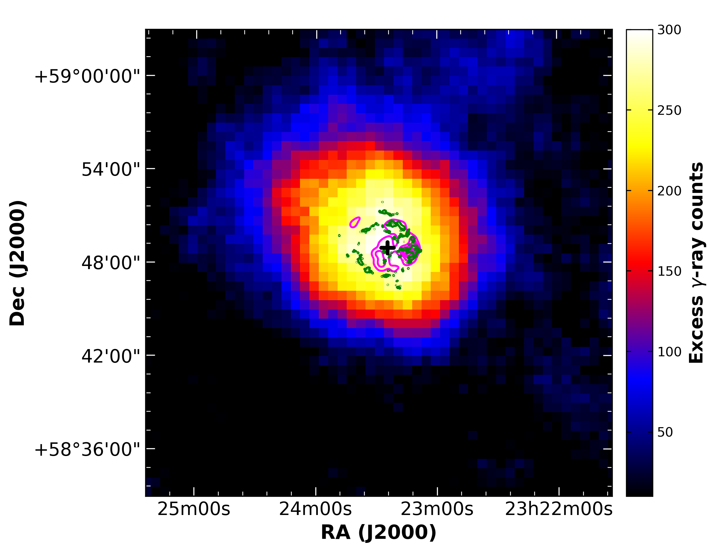
Figure 1: The skymap of excess $\gamma$-ray events (with energy higher than 200 GeV) around the region of Cas A, smoothed with a circular window of radius $0.09^{\circ}$. Magenta and green contours overlaid on this excess map are taken from NuStar $15-20\mathrm{\ keV}$ X-ray emission (Grefenstette et al., 2015) and the VLA $6\mathrm{\ cm}$ radio emission respectively. The black cross indicates the measured centroid position of the $\!\!\mathrm{\ TeV}$ $\gamma$-ray source.

2.2 Spectral analysis

To derive the energy spectrum, the entire Dataset (I, II, III and IV) was used. A total of $1535$ $\gamma$-ray like events ($N_{on}$) were counted from a region of radius $0.09^{\circ}$ around Cas A. Since this region also contain background events, background is obtained by counting the total number of events from $6$ identical source-free regions in the same field of view using reflected region model (Berge et al., 2007). This gives $N_{off}=6241$. By taking into account the ratio of area of on and off regions ($\alpha=0.167$), excess number of $\gamma$-ray events were calculated at a value of $N_{excess}=495\pm 41$. The significance of this detection, calculated using Equation 17 of Li & Ma (1983), was $13.1\sigma$. The excess $\gamma$-ray events are then binned into $9$ equal logarithmically spaced energy bins to obtain the differential energy spectrum (see Table 2). Above the threshold energy of $200\mathrm{\ GeV}$, the spectrum is well-described by a PL distribution (See Figure 2):

$$\frac{dN}{dE}=(1.45\pm 0.11_{stat})\times 10^{-12}({E}/{\rm{TeV}})^{-2.75\pm 0.10_{stat}}\rm{~{}cm^{-2}~{}s^{-1}~{}TeV^{-1}}\,.$$ (1)

A PL fit to the data points gives a $\chi^{2}$ of 2.2 for 5 degrees of freedom, resulting in a fit probability of 81%. This result is in agreement with the previously published HEGRA (Aharonian et al., 2001), VERITAS (Acciari et al., 2010) and MAGIC (Albert et al., 2007) spectral measurements, when both statistical and systematic errors are taken into account. Compared to previously published VERITAS spectral results (Acciari et al., 2010), the present work leads to a reduction of statistical errors on the spectral index and flux normalization by $\sim 60\%$ and $\sim 40\%$ respectively. The differential flux points measured by VERITAS (see Table 2) are also compatible with the recent MAGIC results (Ahnen et al., 2017).

Table 2: Differential spectral flux points with statistical errors from VERITAS data in the energy range $0.2-12.6\mathrm{\ TeV}$. Upper limits of differential flux are obtained at $95\%$ confidence level for those points where significance is less than $2\sigma$.

Energy	Energy min	Energy max	$\mathrm{E^{2}dN(E)/dE}$	Significance
($\mathrm{TeV})$	($\mathrm{TeV}$)	($\mathrm{TeV}$)	($\mathrm{10^{-12}\,erg^{1}\,s^{-1}\,cm^{-2}}$)	($\sigma$)
0.25	0.20	0.32	15.20 (upper limit)	0.1
0.40	0.32	0.50	$4.28_{-0.76}^{+0.79}$	6.1
0.63	0.50	0.79	$3.64_{-0.51}^{+0.53}$	8.1
1.00	0.79	1.26	$2.17_{-0.39}^{+0.40}$	6.3
1.58	1.26	2.00	$1.83_{-0.35}^{+0.37}$	5.9
2.51	2.00	3.16	$1.40_{-0.31}^{+0.34}$	5.3
3.98	3.16	5.01	$0.63_{-0.26}^{+0.29}$	2.7
6.31	5.01	7.94	$0.50_{-0.21}^{+0.25}$	2.8
10.00	7.94	12.59	0.37 (upper limit)	1.0

3 Fermi-LAT: Observations and analysis results

The LAT instrument on board the Fermi satellite is a pair-conversion $\gamma$-ray detector that detects photons in the energy range between 20$\mathrm{\ MeV}$ and $>$ 500$\mathrm{\ GeV}$. The LAT has a field of view of $\sim$2.4$\mathrm{\ sr}$, effective area of $\sim 8200\mathrm{\ cm^{2}}$ on-axis above $1\mathrm{\ GeV}$ (Pass 8 events) and an angular resolution of $\sim 0.8^{\circ}$ at $1\mathrm{\ GeV}$. Full details about the LAT instrument can be found in Atwood et al. (2009).

We analyzed 10.8 years of Pass 8 R3 LAT data (see Atwood et al. (2013) for more details), from 2008 August 4 to 2019 May 31. We used the Fermipy Python package (version 0.17.4, Wood et al. (2017)) that automates the analysis of Pass 8 data in conjuction with the publicly available software fermitools, version 1.0.1. We selected events from a $20^{\circ}\times 20^{\circ}$ region centered on the position of Cas A in the energy range from $100\mathrm{\ MeV}$ to $500\mathrm{\ GeV}$. In order to minimize the contamination from cosmic rays mis-classified as $\gamma$-rays, we selected events belonging to the UltraCleanVeto Class ($evclass=1024$). Data were filtered further by selecting only PSF2 and PSF3 ($evtype=16$ and $32$) event types that give the best angular resolution. For details about the event classes and event types see the Fermi web pages. Once this data selection was made, we applied another cut to select the good time intervals by using (DATA_QUAL) $>0$ && (LAT_CONFIG $==1$). In order to avoid the contamination from photons produced by cosmic ray interactions in the upper atmosphere, we applied a zenith angle cut of $\theta<90^{\circ}$. The remaining photons were binned using the gtbin tool into a spatial bin size of $0.1^{\circ}\times 0.1^{\circ}$ and into 22 equal logarithmically-spaced energy bins.

We applied the likelihood technique to find the parameters of the source of interest, where likelihood is defined as the probability of data given the model. A joint likelihood function was defined in this work by taking the product of the likelihood function of PSF2 and PSF3 type events. The maximization of this likelihood function provided the parameters of the input model. The input model file used in the binned likelihood analysis was created by including all of the background sources within $20^{\circ}$ from the center of the region of interest (ROI) from the 4FGL catalogue (The Fermi-LAT collaboration, 2019). In addition to this, two background diffuse models; Galactic (gll_iem_v07.fits) and extragalactic (iso_P8R3_ULTRACLEANVETO_V2_PSF2_v1.txt, iso_P8R3_ULTRACLEANVETO_V2_PSF3_v1.txt) were also included in the input model, and the normalization was set free for these two models. During the maximum-likelihood fitting of data with gtlike, the normalization and spectral parameters of sources within $3^{\circ}$ from the center of the ROI were set free. The parameters for other sources, located outside of the $3^{\circ}$ radius, were fixed and set at their catalogue values. The instrument response function (IRF) used in our analysis was P8R3_ULTRACLEANVETO_V2.

3.1 Source localization and extension

For source localization in the high-energy band, we selected P8R3 SOURCE class with front plus back type $\gamma$-ray events in the energy range from $10\mathrm{\ GeV}\leq E_{\gamma}\leq 500\mathrm{\ GeV}$. Such a selection provides a good instrument PSF ($\sim 0.1^{\circ}$) and less contamination from the Galactic diffuse emission which dominates below $1\mathrm{\ GeV}$. The best-fit source position in Galactic coordinates was obtained by the Source Localization routine in the Fermipy package. This routine uses a two step method to find the best-fit source position. In the first step, a likelihood map of size $1^{\circ}\times 1^{\circ}$ around the known position of Cas A is generated, and a fit is performed to find the position of the peak likelihood in the map. This position is further refined in the second step by freeing the location parameters of Cas A and redoing the likelihood fitting in a smaller region that encloses the $99\%$ positional uncertainty contour from the first step. The result of this localization analysis gave the best-fit position at RA $=23^{\mathrm{h}}23^{\mathrm{m}}26.5^{\mathrm{s}}$ and Dec $=+58\arcdeg 48\arcmin 59.8\arcsec$, with a $1\sigma$ statistical uncertainty of $0.2\arcmin$. This new position is offset from the previous position given in Yuan et al. (2013) by $0.5\arcmin$, but is compatible with this result because the systematic error in the position due to the alignment of the telescope system and inaccurate description of the PSF of the instrument is estimated to be $0.3\arcmin$. We also performed an extension analysis of the source using the source extension routine in the Fermipy package. We tested the extension of the source by comparing the likelihood of the extended source hypothesis to the point source hypothesis. For the extended source hypothesis, we tested two source morphology models; a 2D symmetric Gaussian model and a radial disk model. Both models yield no significant detection of the extension. With a confidence level of $95\%$, we calculate the upper limit of the source extension to be $2.2\arcmin$ and $2.5\arcmin$ with the 2D Gaussian model and the radial disk model, respectively. These values for the upper limit on the extension are consistent with the size of the SNR ($2.55\arcmin\pm 0.2\arcmin$ Gotthelf et al. (2001)).

3.2 Spectral analysis

The spectral analysis was performed over the full Fermi-LAT energy range of $0.1-500\mathrm{\ GeV}$ using gtlike. Following Yuan et al. (2013), the spectral shape of the emission from Cas A was assumed to be smoothly broken power-law (SBPL; $dN/dE=N_{0}(E/E_{0})^{-\gamma_{1}}(1+(E/E_{b})^{\frac{\gamma_{2}-\gamma_{1}}{\beta}})^{-\beta}$, where $N_{0}$ is the normalization factor, $E_{0}$ is the scale parameter fixed at a value of $1\mathrm{\ GeV}$, $E_{b}$ represents the break energy in the spectrum, $\gamma_{1}$ and $\gamma_{2}$ are the photon indexes before and after the break, and $\beta$ represents the smoothness of the break and is fixed to $0.1$). The parameters for the SBPL model are shown in Table 3 and the differential flux points are shown in Table 4.

Table 3: Fermi-LAT results: smoothly broken power-law model parameters with statistical error.

$N_{0}$	$E_{0}$	$\gamma_{1}$	$\gamma_{2}$	$E_{b}$	$\beta$
($\rm cm^{-2}~{}s^{-1}~{}MeV^{-1}$)	(GeV)			(GeV)
$(6.4\pm 0.7)\times 10^{-12}$	1.0 (fixed)	$1.3\pm 0.2$	$2.1\pm 0.1$	$1.3\pm 0.4$	0.1 (fixed)

For calculating the SED, the energy range from $0.1$ to $500\mathrm{\ GeV}$ was divided into $22$ logarithmically spaced bins. We used the sed method in the Fermipy package, where SED is computed by performing fitting of flux of Cas A in each energy bin independently, using a fixed spectral index of 2, intermediate between the two indices obtained for the smoothly broken power-law fit and consistent with the index obtained from the global fit to a simple power-law. We determined that the resulting SED flux points (given in Table 4) are insensitive to this choice of index by fitting with indices 1.3 and 2.1 instead and finding the points to differ by less than their error bars.

In the fitting process, the normalization of the Galactic diffuse model was also allowed to vary. Table 4 shows the differential flux points in all bins. As mentioned in Yuan et al. (2013), the uncertainty of the modeling of Galactic diffuse emission is the major contribution for the systematic error on the spectral measurements. Therefore, we consider the impact of this component to overall spectrum measurement. To estimate this error, we calculated the discrepancy between the number of counts predicted from the best-fit model and the data at 17 random locations close to the position of Cas A, but away from all known sources (similar to the procedure adopted in Abdo et al. (2009)). The differences between the best-fit model and data were found to be $\sim 5\%$. In order to estimate the systematic error, therefore, we changed the normalization of the Galactic diffuse model artificially by $\pm 5\%$ from the best-fit values. Figure 2 shows the Cas A SED from Fermi-LAT data with systematic and statistical errors. For comparison, SED points from Ahnen et al. (2017), measured by the MAGIC collaboration, are also plotted on Figure 2. All of the SED points from this work are consistent with the published Ahnen et al. (2017) points within 1-2 $\sigma$ considering both statistical and systematic errors .

Table 4: SED points from Fermi-LAT data in the energy range $0.1-500\mathrm{\ GeV}$ (only statistical errors).

Energy	Energy min	Energy max	$\mathrm{E^{2}dN(E)/dE}$	Significance
($\mathrm{GeV})$	($\mathrm{GeV}$)	($\mathrm{GeV}$)	($\mathrm{10^{-12}\,erg^{1}\,s^{-1}\,cm^{-2}}$)	($\sigma$)
0.12	0.10	0.15	$4.60_{-1.35}^{+1.36}$	3.4
0.18	0.15	0.22	$3.10_{-1.08}^{+1.09}$	2.9
0.26	0.22	0.32	$2.11_{-0.96}^{+0.97}$	2.2
0.39	0.32	0.47	$6.09_{-0.88}^{+0.90}$	7.2
0.57	0.47	0.69	$6.74_{-0.78}^{+0.80}$	9.4
0.84	0.69	1.02	$8.81_{-0.75}^{+0.77}$	13.9
1.24	1.02	1.50	$11.60_{-0.79}^{+0.81}$	19.7
1.82	1.50	2.21	$10.60_{-0.78}^{+0.82}$	19.4
2.69	2.21	3.26	$10.90_{-0.85}^{+0.90}$	20.8
3.96	3.26	4.80	$13.40_{-1.05}^{+1.13}$	24.0
5.83	4.80	7.07	$12.00_{-1.21}^{+1.31}$	19.4
8.58	7.07	10.41	$8.31_{-1.18}^{+1.30}$	14.6
12.64	10.41	15.34	$9.75_{-1.50}^{+1.71}$	15.0
18.61	15.34	22.59	$13.40_{-2.08}^{+2.37}$	16.3
27.41	22.59	33.27	$6.62_{-1.73}^{+2.05}$	9.2
40.37	33.27	49.00	$6.30_{-2.01}^{+2.43}$	7.7
59.46	49.00	72.16	$9.04_{-2.88}^{+3.49}$	8.3
87.57	72.16	106.27	$10.30_{-3.74}^{+4.62}$	7.4
128.97	106.27	156.52	$2.61_{-1.98}^{+3.34}$	2.6
189.95	156.52	230.52	$7.93_{-4.84}^{+6.78}$	3.6
279.75	230.52	339.50	$19.60_{-9.74}^{+12.80}$	6.0
412.01	339.50	500.00	$10.80_{-8.11}^{+13.60}$	3.3

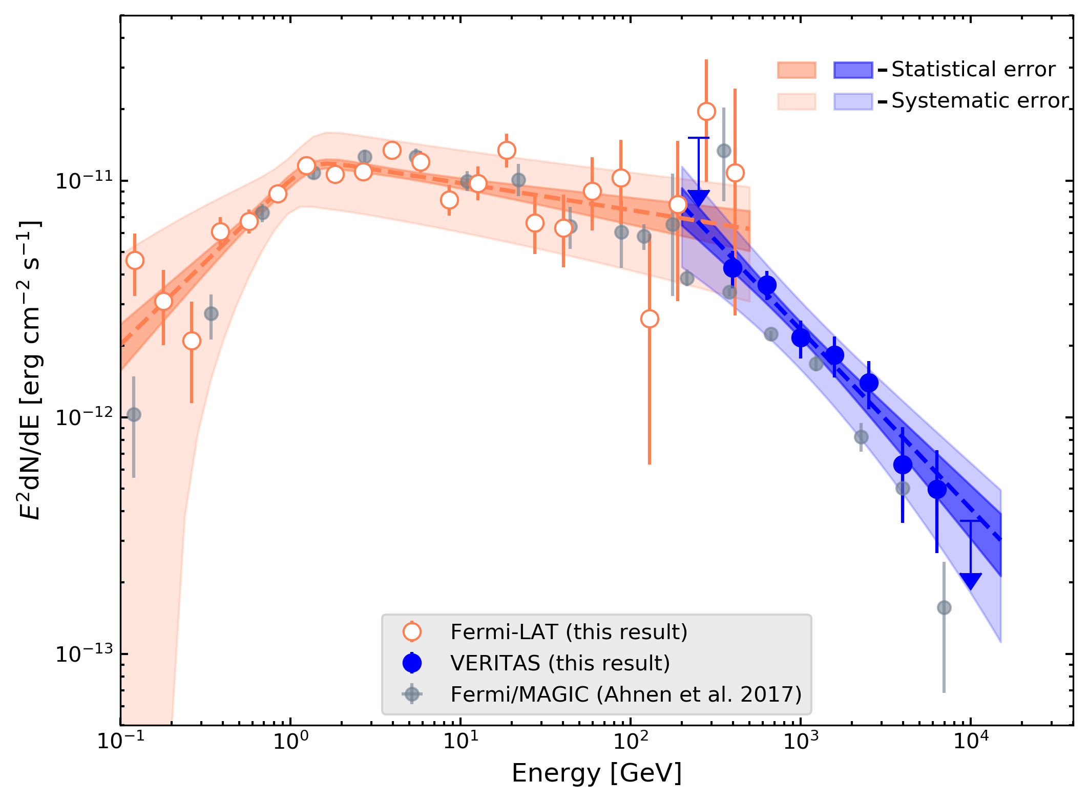
Figure 2: Broadband SED of Cas A using Fermi-LAT and VERITAS points. For comparison, Fermi-LAT/MAGIC SED points measured in Ahnen et al. (2017) are also plotted in grey. Orange (blue) shaded region represents the $1\sigma$ statistical error band on the spectral fit of Fermi-LAT (VERITAS). Similarly, the light-orange (light-blue) shaded region represents $1\sigma$ systematic errors (only; not including statistical errors) for Fermi-LAT (VERITAS). Fermi-LAT points (open orange circles) are fitted with SBPL from $0.1-500\mathrm{\ GeV}$ and VERITAS points (filled blue circles) are fitted with simple power-law from $200-15000\mathrm{\ GeV}$.

4 Combined Fermi-LAT and VERITAS results

4.1 Centroid positions

Figure 3 shows the hard X-ray emission from Cas A measured using NuSTAR telescope in the energy range $15-20\mathrm{\ keV}$ (Grefenstette et al., 2015) with the centroid positions of the $\!\!\mathrm{\ GeV}$ and the $\!\!\mathrm{\ TeV}$ emission. The best-fit positions obtained with the Fermi-LAT and VERITAS are compatible with each other and lie close to the center of the remnant. Because the PSF of Fermi-LAT and VERITAS is comparable to the size of remnant, it is difficult to compare the emission locations for hard X-rays, GeV and TeV $\gamma$-rays. Therefore, a morphological comparison between hard X-ray emission and $\gamma$-ray emission does not help us to interpret the emission mechanism for GeV and TeV $\gamma$-rays at this point.

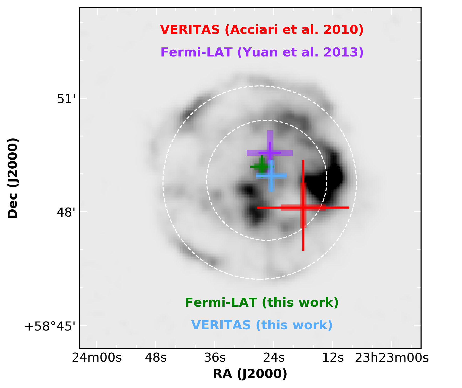
Figure 3: Comparison of $\mathrm{\ GeV}$ and $\mathrm{\ TeV}$ centroid positions. The background image shows the NuSTAR $15-20\mathrm{\ keV}$ hard X-ray emission from Cas A (Grefenstette et al., 2015). The two dashed circles denote the positions of forward and reverse shocks (Gotthelf et al., 2001). Updated VERITAS (for $\gamma$-ray above $200\mathrm{\ GeV}$ energy) and Fermi-LAT (for $\gamma$-ray above $10\mathrm{\ GeV}$ energy) centroid positions are denoted by green and blue crosses. The thick crosses represent $1\sigma$ statistical errors and thin crosses represent $1\sigma$ systematic errors. Also shown here are the best-fit positions from the previous VERITAS (Acciari et al., 2010) and Fermi-LAT observations (Yuan et al., 2013) in red and purple crosses, respectively.

4.2 Broadband spectral fit

Up to this point, we have calculated the flux points from Fermi-LAT and VERITAS data independently using different analysis packages. Here, we take those flux points, assuming that they are independent, and combine them to perform a broadband spectral fit. We performed the broadband fit above the break energy of the Fermi-LAT spectrum to check the spectral behaviour at the highest end of the energy range. The spectral points from the Fermi-LAT (above the spectral break only, i.e. $>1.3\mathrm{\ GeV}$) and VERITAS are fitted jointly using three different models: a single PL, an exponential cut-off power-law (ECPL) and a SBPL. See Table 5 for the formula of each spectral model. The PL fit yields a $\chi^{2}$-fit probability of $3.1\times 10^{-7}$, whereas the ECPL and SBPL yield $\chi^{2}$-fit probabilities of 0.06 and 0.13, respectively. The ECPL and SBPL models are therefore favored over the PL model at the $6.0\sigma$ level when only statistical errors are considered. Adding a systematic error of $0.1_{sys}$ (Yuan et al., 2013) in the Fermi spectral index and $0.2_{sys}$ (Madhavan, 2013) on the VERITAS spectral index, reduces the significance of the ECPL and SBPL over PL to $\sim 4.0\sigma$ level. Since both ECPL and SBPL show similar significance, and ECPL has fewer parameters than SBPL, we take ECPL as the best-fit model for our Dataset. Figure 4 shows the best-fit ECPL model on the joint Fermi-LAT and VERITAS spectral points. The energy of the cut-off is measured to be $2.3\pm 0.5_{stat}\mathrm{\ TeV}$. This value is consistent with the cutoff of $3.5_{-1.0}^{+1.6}\mathrm{\ TeV}$ measured by MAGIC (Ahnen et al., 2017).

Table 5: Comparison of different spectral models for the fit to the Fermi-LAT and VERITAS data above $1.3\mathrm{\ GeV}$.

Spectral Model	Formula	Parameter values	$\chi^{2}$ / ndf
PL	$N_{0}(E/E_{0})^{-\gamma}$	$\gamma=2.30\pm 0.01$	68/20
ECPL	$N_{0}(E/E_{0})^{-\gamma}\exp(-E/E_{c})$	$\gamma=2.17\pm 0.02$	30/19
		$E_{c}\>(\!\!\mathrm{\ TeV})=2.31\pm 0.51$
SBPL	$N_{0}(E/E_{0})^{-\gamma_{1}}(1+(E/E_{b})^{\frac{\gamma_{2}-\gamma_{1}}{\beta}})^{-\beta}$	$\gamma_{1}=2.11\pm 0.04$	25/18
		$\gamma_{2}=2.77\pm 0.10$
		$E_{b}\>(\!\!\mathrm{\ TeV})=0.25\pm 0.09$

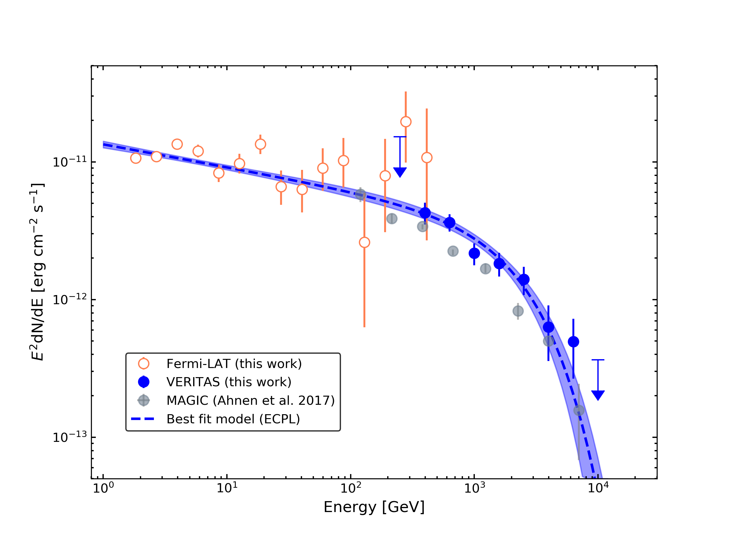
Figure 4: Fermi-LAT and VERITAS measured spectral points of Cas A. Assuming only statistical errors, the best-fit ECPL model is shown with a dotted blue line. The blue shaded region represents the $1\sigma$ statistical error band on the best-fit ECPL spectral model.

5 Theoretical modeling

5.1 Model assumptions

We build a global model to investigate the multi-wavelength spectrum from radio up to the TeV energy range. For simplicity, we assume a one-zone model fixed by two parameters: the ambient hydrogen number density, $n_{\mathrm{H}}$, and the post-shock magnetic-field strength, $B$. Both quantities are assumed constant, i.e. independent of time and location. The differential electron (proton) number densities, $N_{e(p)}$, are assumed to follow ECPL

$$N(p)=N_{0}\,p^{-s}\exp\left(-\frac{p}{p_{cut}}\right)\,.$$ (2)

Here $p$, $p_{cut}$, and $s$ denote the electron (proton) momentum, the cut-off momentum and the PL index of the spectrum, respectively, all of which are free parameters of our model. The normalization, $N_{0}$, in principle reflects the injection efficiency of each particle species. We calculate the synchrotron emission from the non-thermal electron spectrum (Blumenthal & Gould, 1970), taking into account the modifications caused by the turbulent component of the magnetic field (Pohl et al., 2015). NTB and IC radiation, which can significantly contribute to the $\gamma$-ray spectrum of SNR, are also obtained from the non-thermal electron distribution. For the IC interactions (Blumenthal & Gould, 1970), we consider two target photon fields: the cosmic microwave background and the infrared emission from the shock-heated ejecta with temperature $\sim 100\,\mathrm{K}$ and energy density $2\,\mathrm{eV\,cm}^{-3}$ (Mezger et al., 1986). The NTB contribution from relativistic electrons follows the calculations of Blumenthal & Gould (1970). Additionally, thermal bremsstrahlung from plasma electrons is included assuming local thermodynamic equilibrium (Hnatyk & Petruk, 1999). The $\gamma$-ray yield from protons via neutral-pion decay is computed using the procedure of Huang et al. (2007). Including the hydrogen number density and the magnetic field strength, we have in total nine independent parameters in our global model. The parameters are shown in Table 6. The hydrogen number density, $n_{\mathrm{H}}$, corresponds to the upstream value and magnetic-field strength, $B$, to the downstream region. In the following, we consider two scenarios: a hadron-dominated model and a lepto-hadronic case, which we refer to as Model I and II, respectively.

Table 6: Parameters for theoretical models.

	Varying parameters					Same for both models
Model	$B$	$N_{0,e}$	$N_{0,p}$	$p_{cut,e}$	$p_{cut,p}$	$s_{e}$	$s_{p}$	$T_{e}$	$n_{\mathrm{H}}$
	($\mathrm{\mu G}$)	$(\mathrm{(m_{e}c)^{s_{e}-1}})$	$(\mathrm{(m_{p}c)^{s_{p}-1}})$	($\mathrm{m_{e}c}$)	($\mathrm{m_{p}c}$)			($10^{7}$K)	($\mathrm{cm^{-3}}$)
I	450	$4.2\times 10^{13}$	$3.2\times 10^{23}$	$9.0\times 10^{6}$	$2.1\times 10^{4}$	2.5	2.17	1.8	1.0
II	150	$2.9\times 10^{14}$	$3.8\times 10^{23}$	$1.6\times 10^{7}$	$6.0\times 10^{3}$	2.5	2.17	1.8	1.0

5.2 Hadronic model

We start with a purely hadronic model of the $\gamma$-ray emission from Cas A. Using Equation 2 we find the best-fit for the joint Fermi-LAT and VERITAS data points, shown in Figure 5. The corresponding best-fit parameters, with $\frac{\chi^{2}}{d.o.f.}=1.38$, are $s_{p}=2.17$ and $p_{cut}=2.1\times 10^{4}\,\mathrm{m_{p}c}$ (equivalent to $E_{cut}\approx 17\,\mathrm{TeV}$). More instructive than the best-fit model are the confidence regions of the parameters, revealed by $\mathrm{\Delta\chi^{2}=\chi^{2}-\chi^{2}_{min}}$. Therefore, we scan the $s_{p}-p_{cut,p}$ parameter space and calculate $\Delta\chi^{2}$ while optimizing $N_{0}$. The results are shown in Figure 6. Here the dark-blue area represents $\mathrm{\Delta\chi^{2}<2.30}$, medium-blue $\mathrm{\Delta\chi^{2}<6.18}$ and the light-blue $\mathrm{\Delta\chi^{2}<11.83}$, which corresponds to $1\sigma$, $2\sigma$ and $3\sigma$, respectively (Lampton et al., 1976). As seen from Figure 6, the canonical solution from DSA theory ($s=2.0$) is excluded with $>99.7\%$ confidence. Thus, in the case of a hadronic origin, the $\gamma$-ray data mandate a proton spectral index ($s_{p}\approx 2.1-2.2$) softer than predicted by the standard DSA theory ($s=2.0$) or nonlinear DSA ($s<2.0$ at $p\gg mc$) (Malkov & Drury, 2001). Figure 6 indicates a cut-off with $p_{cut,p}\sim 10^{4}\,\mathrm{m_{p}c}$, in full agreement with Ahnen et al. (2017), who concluded that Cas A is not a PeVatron.

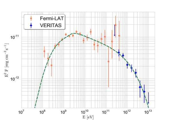
Figure 5: Purely hadronic best-fit with $\chi^{2}=36.01$ and $d.o.f.=26$ ($\chi^{2}/d.o.f.=1.38$). The corresponding best-fit parameters following Equation. 2 are $s_{p}=2.17$ and $p_{cut}=2.1\times 10^{4}\,\mathrm{m_{p}c}$ .

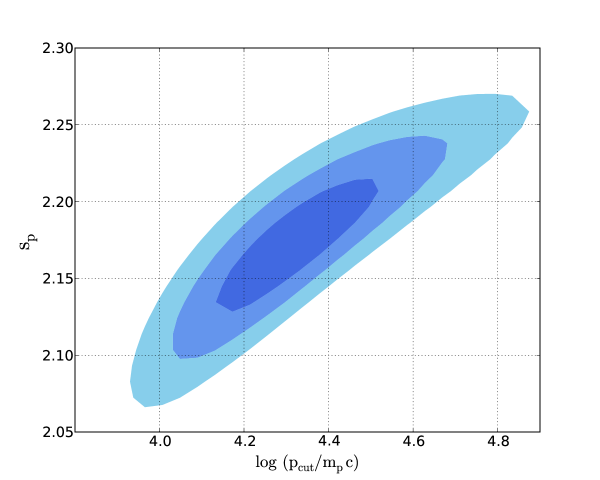
Figure 6: Purely hadronic model: The confidence regions for the spectral index, $s$, and cut-off momentum, $p_{cut}$. The dark-blue area corresponds to 68.3% probability, or 1$\sigma$, medium-blue to 95.5%, or 2$\sigma$, and the light-blue field to 99.7%, or 3$\sigma$, respectively.

In the next step, we determine the electron spectrum for the global model of the broadband emission. The electron power-law index, $s_{e}\approx 2.5$, is entirely fixed by the radio data (Vinyaikin, 2014), and the X-ray flux (Maeda et al., 2009) is well explained by the synchrotron cut off. A minor discrepancy occurs above 100 keV where the INTEGRAL spectral data (Wang & Li, 2016) suggest a spectral hardening, which might reflect an asymmetric explosion (Wang & Li, 2016) and thus cannot be included in our modeling. An alternative explanation involves weakly relativistic electrons emitting NTB, as we discuss in Section 5.3.

Lee et al. (2014) found that the upstream gas density for Cas A lies in the range 0.6 to 1.2 cm^-3. In this work we follow Lee et al. (2014) and use $n_{\mathrm{H}}=1.0\,\mathrm{cm^{-3}}$ for simplicity. In order for the IC component not to dominate the $\gamma$-ray production from hadrons, the magnetic field in the downstream region needs to be at least $\sim$450 $\mu$G, and we use this minimum value in the model. This magnetic-field strength is compatible with the results of Zirakashvili et al. (2014) and Sato et al. (2018) who argued that for Cas A, $B\sim 0.5-1\,\mathrm{mG}$. For a magnetic field this strong ($\sim$450 $\mu$G) the thickness of the X-ray rims must reflect synchrotron energy losses of the radiating electrons (Parizot et al., 2006).

The entire SED is presented in Figure 7, and the corresponding model parameters are summarized in Table 6 (Model I). The hadronic component (green dashed line) is the best-fit spectrum presented in Figure 5. Besides the marginal IC contribution, we obtain a negligible NTB component, which we calculate starting from 10 MeV. While the spectral shape of the electrons for energies above $\sim$100 MeV can be constrained by the radio data, no data exist to test the spectral shape for electrons with energies below $\sim$100 MeV. Consequently, accurate modeling of the NTB radiation below $\sim$10 MeV, which corresponds to $\sim$100 MeV electron energy, is not possible. Therefore, in our modeling the total photon spectrum disconnects between 100 keV and 10 MeV. The electron temperature, $T_{e}$, is chosen according to Maeda et al. (2009), and the thermal-bremsstrahlung emission provides a moderate contribution to the X-ray flux. The main reason for the rather insignificant thermal and NTB contributions is a relatively low plasma density in the downstream region given for a strong shock by $n_{\mathrm{H,d}}=4n_{\mathrm{H}}$.

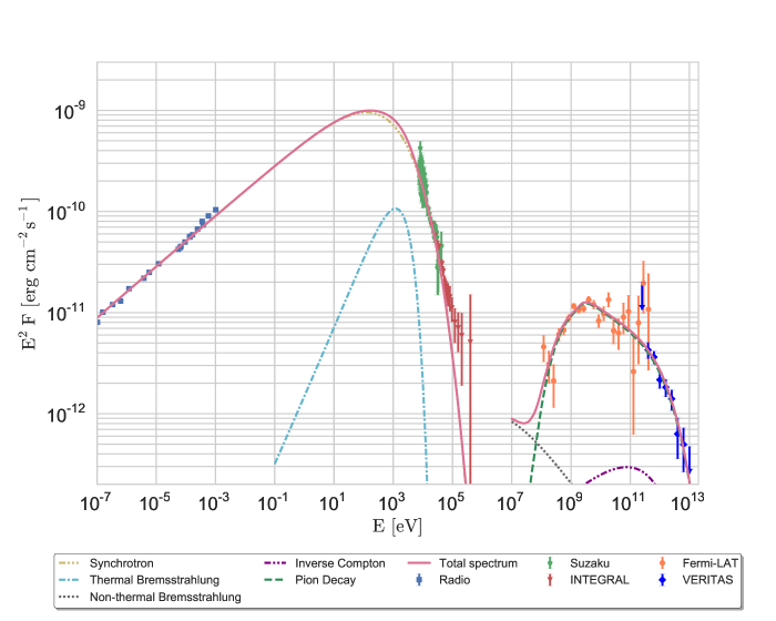
Figure 7: Model I: Hadronic model with downstream magnetic field $B\approx 450\,\mathrm{\mu G}$ and upstream gas density $\mathrm{n_{H}}=1\,\mathrm{cm^{-3}}$. The radio data are taken from Vinyaikin (2014); X-ray data from Maeda et al. (2009) and Wang & Li (2016).

Finally, we test if the increasing $\gamma$-ray flux at $\sim$100 MeV can be explained by NTB. Indeed, at first glance the two lowest-energy Fermi data points suggest the presence of an additional emission besides the pion bump, such as NTB. Performing the $\chi^{2}$-test after taking into account both NTB and neutral-pion decay, we find, however, that a negligible NTB contribution is preferred. The corresponding best-fit with $\frac{\chi^{2}}{d.o.f.}=1.42$ is presented in Figure 8. Nevertheless, Cas A has been considered for a long time as the best candidate for detecting NTB (Cowsik & Sarkar, 1980; Allen et al., 2008). Therefore, we investigate the possibility of a lepto-hadronic model for the observed $\gamma$-ray spectrum of Cas A in the following section.

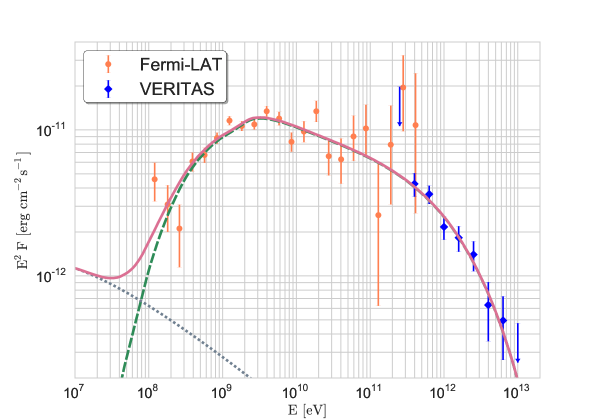
Figure 8: Best-fit for the hadronic component (green dashed line) plus non-thermal bremsstrahlung (blue dotted line); the total spectrum (pink solid line) with $\chi^{2}=35.50$ and $d.o.f.=25$ ($\chi^{2}/d.o.f.=1.42$).

5.3 Lepto-hadronic model

In this section we determine the observable limits on the presence of NTB and establish a model with a maximum possible NTB contribution.

In the framework of our one-zone model, NTB at a few hundred MeV is emitted by the same electrons that produce radio synchrotron emission at a few hundred MHz, and so a flux comparison between the radio data and the Fermi points at $\sim$100 MeV, ($F_{\mathrm{1\,GHz}}/F_{\mathrm{100\,MeV}}$), determines the relation between the average gas density and the minimum magnetic-field strength. Choosing the pre-shock gas density according to Lee et al. (2014), $n_{\mathrm{H}}=1.0\,\mathrm{cm^{-3}}$, we obtain for the minimum downstream magnetic-field strength: $B_{\mathrm{min}}\approx 150\,\mathrm{\mu G}$. Any weaker magnetic field would lead to NTB overshooting of the data points at $\sim$100 MeV.

In general, the emission coefficients for synchrotron and NTB scale with magnetic-field strength and gas number density, respectively, as

$$j_{sy}\propto B^{\frac{1+s_{e}}{2}}\qquad\qquad\textrm{and}\qquad\qquad j_{ntb}\propto n_{\mathrm{H}}\,.$$ (3)

Therefore, to sustain constant synchrotron and NTB-flux ratio, the following condition for downstream magnetic field and ambient hydrogen number density has to be fulfilled:

$$\left(\frac{B}{150\,\mathrm{\mu G}}\right)^{\frac{1+s_{e}}{2}}=\left(\frac{n_{\mathrm{H}}}{1\,\mathrm{cm}^{-3}}\right)\ .$$ (4)

Aside from this case, the NTB component becomes suppressed with increasing magnetic field but constant gas density. Starting from some critical magnetic-field value the overall $\gamma$-emission becomes hadron dominated, as discussed in Section 5.2. The minimum post-shock magnetic field for Cas A is therefore given by

$$B\gtrsim 150\ \mathrm{\mu G}\,\left(\frac{n_{\mathrm{H}}}{\mathrm{cm}^{-3}}\right)^{\frac{2}{1+s_{e}}}\,,$$ (5)

as can be recognized from Equation 4. The minimum magnetic field deduced from potential NTB contribution depends on the ambient density of the remnant. The density uncertainties provided by Lee et al. (2014), suggest that the minimum magnetic-field value may vary from $110\,\mathrm{\mu G}$ to $170\,\mathrm{\mu G}$.

Having established the strength of the magnetic field inside Cas A, we immediately find several consequences. First, given the age of the remnant, $\sim 10^{10}$ s, only electrons with Lorentz factors $\gamma\gg 10^{6}$ can be affected by energy losses. The resulting IC peak, which is calculated from a combination of CMB and FIR target-photon fields, would lie near $100$ GeV in the spectrum, and its spectral shape would be incompatible with that measured in the GeV band. The second consequence is that the peak energy flux of the IC component must be about a factor $U_{\mathrm{mag}}/(U_{\mathrm{cmb}}+U_{\mathrm{fir}})\simeq 250$ lower than that of the near-UV synchrotron emission radiated by the same electrons (Pohl, 1996). Consequently, the IC peak at 100 GeV is roughly a factor of 3 below the observed $\gamma$-ray flux and thus, IC emission alone can hardly provide the bulk of the $\gamma$-ray emission at $100$ GeV. It does contribute to a significant part of it though, and the highest-energy TeV emission is fully accounted for by the highest-energy IC contribution. Both points indicate that an additional radiation component, such as from neutral-pion decay, is required. Therefore, we conclude that a purely leptonic model is very unlikely.

The lepto-hadronic case (Model II) with a maximum possible NTB component that is consistent with the Fermi data points is shown in Figure 9. The IC peak (purple dash-dot-dotted line) located at $\sim$100 GeV sets an additional constraint on the magnetic field inside Cas A. Decreasing the magnetic field would enhance the IC contribution, which would exceed the TeV-flux measured with VERITAS (blue diamond-shaped points in Figure 9). Thus, both IC and NTB provide the same lower limit for the post-shock magnetic field, $\sim 150\,\mathrm{\mu G}$. In contrast to NTB, IC does not scale with the gas density. Therefore, it provides an independent constraint on the magnetic-field value and implies that $B<150\,\mathrm{\mu G}$ is highly unlikely for Cas A.

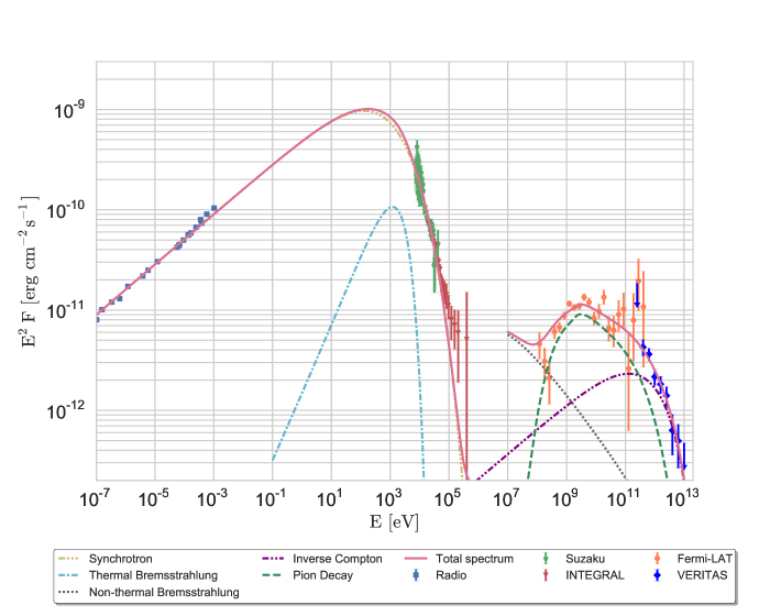
Figure 9: Model II: Lepto-hadronic model with a minimum post-shock magnetic field $B\approx 150\,\mathrm{\mu G}$ and ambient gas density $\mathrm{n_{H}}=1\,\mathrm{cm^{-3}}$. The radio data are taken from Vinyaikin (2014); X-ray data from Maeda et al. (2009) and Wang & Li (2016).

Despite a significant NTB contribution, $\gamma$-ray data in the GeV and higher MeV band are adequately explained by the pion bump and the discrimination between lepto-hadronic and purely hadronic models remains vague. Table 6 presents the parameters for the global lepto-hadronic model (Model II). The normalization factor, $N_{0,e}$, and the cut-off momentum of the electron spectrum, $p_{cut,e}$, are readjusted to fit the radio data for the weaker magnetic field. Since the cut off at TeV energies is largely reproduced by the IC, the proton spectrum cuts off already at roughly 6 TeV. Alternatively, the hadronic contribution at TeV energies can be reduced by assuming the proton spectral index softer than 2.17.

An advantage of the lepto-hadronic model is a possible explanation for the hardening of the X-ray spectrum above 100 keV observed with INTEGRAL (Wang & Li, 2016) by emission from non-relativistic electrons radiating NTB. This idea is supported by the findings of Allen et al. (2008), who analyzed the X-ray data of Cas A and concluded that, in the energy range 10-32 keV, NTB exceeds the synchrotron radiation by a factor 2 to 3. A logical extrapolation is that the non-relativistic electrons that are not in thermal equilibrium can provide a significant NTB contribution in the range 100 keV - 1 MeV and thus explain the hard X-ray spectrum. As mentioned above, we do not model this explicitly because we lack the exact shape of the electron spectrum at lower energies.

Note that, in contrast to the hadron-dominated model, in which we are able to use a chi-squared fit to the $>$100 MeV data, we follow a ”fit by eye” process (as for example in Zhang & Liu (2019)) for the lepto-hadronic scenario. The lepto-hadronic scenario includes the NTB and IC components and needs to incorporate the entire SED, making a formal fit and interpretation of the chi-squared from multiple instruments with very different statistical and systematic errors considerably more challenging. We have also chosen a case with the minimum possible magnetic field inside Cas A, which, as described above, provides the maximal (not best-fit) leptonic contributions.

5.4 Discussion

The observed radio spectrum of Cas A constrains the spectral index of the electrons to be $s_{e}\approx 2.5$, and the $\gamma$-ray data favor a softer proton spectrum, $s_{p}\approx 2.17$, than predicted by DSA. One possible explanation involves effects arising from turbulence growth and damping (Malkov et al., 2011; Brose et al., 2016). Alternatively, quasi-perpendicular shocks in young SNRs can steepen the spectral index (Bell et al., 2011). In the case of a young core-collapse SNR like Cas A, the hydrodynamical structure of the progenitor wind zone and acceleration at the reverse shock can significantly modify the particle spectra (Atoyan et al., 2000; Telezhinsky et al., 2013; Zirakashvili et al., 2014). The detection of X-ray synchrotron radiation in the interior of Cas A suggests particle acceleration at the reverse shock (Gotthelf et al., 2001; Uchiyama & Aharonian, 2008; Helder & Vink, 2008). However, newer data indicate that essentially all of the $>15\mathrm{\ keV}$ synchrotron flux is produced in small knots located in the 3D interior of the remnant, rather than a surface like the reverse shock (Grefenstette et al., 2015). Finally, stochastic re-acceleration of electrons behind the forward shock may be able to soften the spectrum over 3 decades in synchrotron frequency (Pohl et al., 2015). In the present work, we follow a simple procedure to address the most important conclusions: determination of the minimum magnetic field strength; confirmation of the pion bump and the corresponding proton cut-off energy. More sophisticated models (including, e.g., asymmetric explosion, time-dependent hydrodynamic simulations, acceleration at the reverse shock, magnetic turbulence and stochastic re-acceleration of particles) are needed, to further differentiate between competing scenarios concerning particle acceleration in SNRs.

The total cosmic ray energy for the hadron-dominated (Model I) and lepto-hadronic (Model II) models considered here is found to be $E_{\mathrm{CR}}\approx 1.7\times 10^{50}$ erg and $E_{\mathrm{CR}}\approx 1.2\times 10^{50}$ erg, respectively. These numbers roughly represent the total energy that went into the particles as they accumulated over the entire evolution time of the remnant. Unfortunately, there is no easy way to ascertain the original explosion energy of Cas A, $E_{\mathrm{SN}}$: the estimations vary between 2$\times 10^{51}$ erg and 5$\times 10^{51}$ erg (Laming & Hwang, 2003; Chevalier & Oishi, 2003; Schure et al., 2008; Lee et al., 2014; Orlando et al., 2016). This suggests that the fraction of the explosion energy expended in accelerating particles is between 2% and 9%. Being a very young SNR, Cas A is very likely in the ejecta-dominated phase (Morse et al., 2004), implying that only a fraction of its explosion energy can be currently extracted from the shock. The full energy becomes available after the SNR enters the Sedov-Taylor stage. In that case, the above numbers may not indicate accurately the acceleration efficiency of the remnant. Truelove & McKee (1999) suggested that Cas A is in transition from the ejecta-dominated to the Sedov-Taylor stage. To verify this, we follow calculations in Dwarkadas (2013), who assumed that Cas A is still in the free-expansion phase and expands into a wind with density profile $\rho\propto r^{-2}$. The maximum shock energy that is available for particle acceleration is found to be:

$$E_{\mathrm{acc}}=\frac{2\pi m^{3}}{(3m-2)}\,\frac{\rho_{\mathrm{u}}R_{\mathrm{sh}}^{5}}{t_{\mathrm{age}}^{2}}\qquad\textrm{with}\qquad m=\frac{(n-3)}{(n-2)}\,.$$ (6)

Here $\rho_{\mathrm{u}}$ is pre-shock gas density, $R_{\mathrm{sh}}$ is shock radius and $t_{\mathrm{age}}$ is age of the remnant. The expansion parameter, defined as $m=d\ln{R_{\mathrm{sh}}}/{d\ln{t}}$, is fixed by the ejecta-density profile, $\rho_{\mathrm{ej}}\propto r^{-n}$, with $n>5$ (e.g. Chevalier, 1982). A reasonable value for $n$ is given by Matzner & McKee (1999) who find that a red supergiant star with a radiative envelope has $n\approx 10$. Assuming this ejecta profile and taking typical values for Cas A: $R_{\mathrm{sh}}=2.5$ pc, $\rho_{\mathrm{u}}=2.34\times 10^{-24}\,\mathrm{g\,cm^{-3}}$ and $t_{\mathrm{age}}=350$ years, we obtain the maximum shock energy available at $E_{\mathrm{acc}}\approx 3.5\times 10^{51}\,\mathrm{erg}$. This result shows that the maximum energy available for particle acceleration in the ejecta-dominated phase is of the same order as the total explosion energy of Cas A, $E_{\mathrm{SN}}\approx 2\times 10^{51}-5\times 10^{51}$ erg, that is presented in literature (Laming & Hwang, 2003; Chevalier & Oishi, 2003; Schure et al., 2008; Lee et al., 2014; Orlando et al., 2016). This indicates that a large fraction of the explosion energy is available at the shock front. Therefore, Cas A is not far from the Sedov-Taylor stage. Our estimation of $2\%-9\%$ of explosion energy is thus appropriate. Further, $E_{\mathrm{acc}}\approx 3.5\times 10^{51}\,\mathrm{erg}$ implies that the acceleration efficiency (defined as $\eta=E_{\mathrm{CR}}/E_{\mathrm{acc}}$) is $\eta\approx 0.05$ and $\eta\approx 0.03$ for hadronic and lepto-hadronic scenarios, respectively. However, one should treat these conclusions with caution, since the values we used for the parameters in Equation 6 are not precisely known. Our result is consistent with the total cosmic ray energy $\sim 9.9\times 10^{49}$ erg presented by the MAGIC collaboration (Ahnen et al., 2017) and exceeds the value $\sim 4\times 10^{49}$ erg found using Fermi-LAT (Yuan et al., 2013).

We find that IC and NTB obviously cannot account for the emission around 10 GeV, and thus a hadronic component is clearly needed. The maximum energies obtained for protons are 21 TeV and 6 TeV for the purely hadronic and lepto-hadronic models, respectively. These values are similar to the previous results of Yuan et al. (2013) (10 TeV) and Ahnen et al. (2017)(12 TeV).

6 Conclusions

In this work, we have presented a deep study of the supernova remnant Cas A using 10.8 years of Fermi-LAT and 65 hours of VERITAS data. The centroid positions from Fermi-LAT and VERITAS measurements are found to be consistent, within errors, and lie inside the remnant. Since the size of the remnant is comparable to the PSF of the Fermi-LAT and VERITAS instruments, it is difficult to determine whether the emission is coming from the forward or the reverse shock within the SNR. More sensitive instruments, in the future, such as the Cherenkov Telescope Array (CTA) (Acharya et al., 2013), will allow us to perform better measurements on the morphology of this source. Above $100\mathrm{\ MeV}$, a spectral index change from $1.3$ to $2.1$ is measured at an energy of $1.3\pm 0.4\mathrm{\ GeV}$ with the Fermi-LAT data, which is consistent with previous observations (Yuan et al., 2013) and can be explained by $\gamma$-ray emission produced through neutral-pion decay. In addition, a joint spectral fit of Fermi-LAT and VERITAS spectral data from $\sim 2\mathrm{\ GeV}$ to $10\mathrm{\ TeV}$ prefers an exponential cut-off power-law to a single power-law model. The cut-off energy found using Fermi-LAT and VERITAS data is estimated to be $2.3\pm 0.5\mathrm{\ TeV}$. This is compatible with the cut-off energy found by the MAGIC collaboration using only MAGIC data (Ahnen et al., 2017). This shows that the Cas A SNR is unlikely to be a source of PeV cosmic rays.

In the theoretical part of this work we took radio (Vinyaikin, 2014) and X-ray (Maeda et al., 2009; Wang & Li, 2016) observations into account. Considering the entire multi-wavelength spectrum of Cas A, we used a global one-zone model assuming power-law particle spectra with an exponential cut off. Two different scenarios, a hadron-dominated case (Model I) and a lepto-hadronic model (Model II) are presented. Furthermore, in agreement with previous studies on the SED of Cas A (Araya & Cui, 2010; Saha et al., 2014); a purely leptonic model is excluded under the assumption of a one-zone scenario, leading to the conclusion that proton acceleration up to TeV energies is clearly evident. The resulting pion bump reflects a slightly softer spectral index for the proton spectrum, $s_{p}\approx 2.17$, than the canonical DSA predictions (both linear and non-linear versions (Malkov & Drury, 2001)). We exclude the canonical DSA solution of $s=2.0$ with $3\sigma$ confidence. The total energy converted into cosmic rays is at least $10^{50}$ erg, giving an acceleration efficiency $\eta\approx 0.03-0.05$.

Although Cas A is the best SNR candidate for NTB emission (Cowsik & Sarkar, 1980; Allen et al., 2008), our observations do not indicate any evidence for a NTB flux above 100 MeV. A clear determination may be achieved with the photon measurements extended down to the MeV energy range. Future experiments, such as AMEGO (All-Sky Medium Energy Gamma-ray Observatory), may shed light on that issue. Nevertheless, assuming a potential NTB presence in Cas A, we set a minimum value for the magnetic-field strength inside the remnant $B_{\mathrm{min}}\approx 150\,\mathrm{\mu G}$. This value is independently confirmed by the IC peak. Therefore, it is clear that the magnetic field inside the Cas A SNR is efficiently amplified, when compared to the interstellar-medium field.

References

- Abdo et al. (2009) Abdo, A. A., et al. 2009, ApJ, 706, L1
- Abdo et al. (2010) Abdo, A. A., et al. 2010, ApJ, 710, L92
- Acciari et al. (2008) Acciari, V. A., et al. 2008, ApJ, 679, 1427
- Acciari et al. (2010) Acciari, V. A., et al. 2010, ApJ, 714, 163
- Acharya et al. (2013) Acharya, B. S., Actis, M., Aghajani, T., et al. 2013, Astroparticle Physics, 43, 3
- Ackermann et al. (2013) Ackermann, M., et al. 2013, Science, 339, 807
- Aharonian et al. (2001) Aharonian, F., et al. 2001, A&A, 370, 112
- Ahnen et al. (2017) Ahnen, M. L., et al. 2017, MNRAS, 472, 2956
- Albert et al. (2007) Albert, J., et al. 2007, A&A, 474, 937
- Allen et al. (2008) Allen, G. E., Stage, M. D., & Houck, J. C. 2008, International Cosmic Ray Conference, 2, 839
- Araya & Cui (2010) Araya, M., & Cui, W. 2010, ApJ, 720, 20
- Atoyan et al. (2000) Atoyan, A. M., Aharonian, F. A., Tuffs, R. J., & Völk, H. J. 2000, A&A, 355, 211
- Atwood et al. (2013) Atwood, W., Albert, A., Baldini, L., et al. 2013, ArXiv e-prints, arXiv:1303.3514
- Atwood et al. (2009) Atwood, W. B., Abdo, A. A., Ackermann, M., et al. 2009, ApJ, 697, 1071
- Axford et al. (1977) Axford, W. I., Leer, E., & Skadron, G. 1977, International Cosmic Ray Conference, 11, 132
- Baade & Zwicky (1934) Baade, W., & Zwicky, F. 1934, Physical Review, 46, 76
- Baars et al. (1977) Baars, J. W. M., Genzel, R., Pauliny-Toth, I. I. K., & Witzel, A. 1977, A&A, 61, 99
- Bell (1978a) Bell, A. R. 1978a, MNRAS, 182, 147
- Bell (1978b) Bell, A. R. 1978b, MNRAS, 182, 443
- Bell et al. (1975) Bell, A. R., Gull, S. F., & Kenderdine, S. 1975, Nature, 257, 463
- Bell et al. (2011) Bell, A. R., Schure, K. M., & Reville, B. 2011, MNRAS, 418, 1208
- Berge et al. (2007) Berge, D., Funk, S., & Hinton, J. 2007, A&A, 466, 1219
- Blandford & Ostriker (1978) Blandford, R. D., & Ostriker, J. P. 1978, ApJ, 221, L29
- Blumenthal & Gould (1970) Blumenthal, G. R., & Gould, R. J. 1970, Rev. Mod. Phys., 42, 237
- Braun et al. (1987) Braun, R., Gull, S. F., & Perley, R. A. 1987, Nature, 327, 395
- Brose et al. (2016) Brose, R., Telezhinsky, I., & Pohl, M. 2016, A&A, 593, A20
- Chevalier (1982) Chevalier, R. A. 1982, ApJ, 258, 790
- Chevalier & Oishi (2003) Chevalier, R. A., & Oishi, J. 2003, ApJ, 593, L23
- Cogan (2008) Cogan, P. 2008, International Cosmic Ray Conference, 3, 1385
- Cowsik & Sarkar (1980) Cowsik, R., & Sarkar, S. 1980, Mon. Not. Roy. Astron. Soc., 191, 855
- Degrange & Fontaine (2015) Degrange, B., & Fontaine, G. 2015, Comptes Rendus Physique, 16, 587 , gamma-ray astronomy / Astronomie des rayons gamma
- DeLaney et al. (2014) DeLaney, T., Kassim, N. E., Rudnick, L., & Perley, R. A. 2014, ApJ, 785, 7
- Dwarkadas (2013) Dwarkadas, V. V. 2013, MNRAS, 434, 3368
- Fesen et al. (2006) Fesen, R. A., Hammell, M. C., Morse, J., et al. 2006, ApJ, 645, 283
- Fomin et al. (1994) Fomin, V. P., Stepanian, A. A., Lamb, R. C., et al. 1994, Astroparticle Physics, 2, 137
- Freeman et al. (2001) Freeman, P., Doe, S., & Siemiginowska, A. 2001, in Proc. SPIE, Vol. 4477, Astronomical Data Analysis, ed. J.-L. Starck & F. D. Murtagh, 76–87
- Gerardy & Fesen (2001) Gerardy, C. L., & Fesen, R. A. 2001, AJ, 121, 2781
- Ginzburg & Syrovatskiĭ (1966) Ginzburg, V. L., & Syrovatskiĭ, S. I. 1966, Soviet Physics Uspekhi, 9, 223
- Gotthelf et al. (2001) Gotthelf, E. V., Koralesky, B., Rudnick, L., et al. 2001, ApJ, 552, L39
- Grefenstette et al. (2015) Grefenstette, B. W., et al. 2015, ApJ, 802, 15
- Helder & Vink (2008) Helder, E. A., & Vink, J. 2008, ApJ, 686, 1094
- Hnatyk & Petruk (1999) Hnatyk, B., & Petruk, O. 1999, Astron. Astrophys., 344, 295
- Holder et al. (2006) Holder, J., et al. 2006, Astroparticle Physics, 25, 391
- Holt et al. (1994) Holt, S. S., Gotthelf, E. V., Tsunemi, H., & Negoro, H. 1994, PASJ, 46, L151
- Huang et al. (2007) Huang, C.-Y., Park, S.-E., Pohl, M., & Daniels, C. D. 2007, Astroparticle Physics, 27, 429
- Hwang et al. (2004) Hwang, U., Laming, J. M., Badenes, C., et al. 2004, The Astrophysical Journal Letters, 615, L117
- Jones et al. (2003) Jones, T. J., Rudnick, L., DeLaney, T., & Bowden, J. 2003, ApJ, 587, 227
- Kassim et al. (1995) Kassim, N. E., Perley, R. A., Dwarakanath, K. S., & Erickson, W. C. 1995, ApJ, 455, L59
- Kieda et al. (2013) Kieda, D., et al. 2013, ArXiv e-prints, arXiv:1308.4849
- Krause et al. (2008) Krause, O., Birkmann, S. M., Usuda, T., et al. 2008, Science, 320, 1195
- Krymskii (1977) Krymskii, G. F. 1977, Akademiia Nauk SSSR Doklady, 234, 1306
- Kumar et al. (2015) Kumar, S., et al. 2015, ArXiv e-prints, arXiv:1508.07453
- Laming & Hwang (2003) Laming, J. M., & Hwang, U. 2003, The Astrophysical Journal, 597, 347
- Lampton et al. (1976) Lampton, M., Margon, B., & Bowyer, S. 1976, ApJ, 208, 177
- Lee et al. (2014) Lee, J.-J., Park, S., Hughes, J. P., & Slane, P. O. 2014, ApJ, 789, 7
- Li & Ma (1983) Li, T.-P., & Ma, Y.-Q. 1983, ApJ, 272, 317
- Madhavan (2013) Madhavan, A. 2013, PhD thesis, Iowa State University
- Maeda et al. (2009) Maeda, Y., et al. 2009, Publ. Astron. Soc. Jap., 61, 1217
- Maier & Holder (2017) Maier, G., & Holder, J. 2017, ArXiv e-prints, arXiv:1708.04048
- Malkov et al. (2011) Malkov, M. A., Diamond, P. H., & Sagdeev, R. Z. 2011, Nature Communications, 2, 194
- Malkov & Drury (2001) Malkov, M. A., & Drury, L. O. 2001, Reports on Progress in Physics, 64, 429
- Matzner & McKee (1999) Matzner, C. D., & McKee, C. F. 1999, ApJ, 510, 379
- Mezger et al. (1986) Mezger, P. G., Tuffs, R. J., Chini, R., Kreysa, E., & Gemuend, H.-P. 1986, A&A, 167, 145
- Morse et al. (2004) Morse, J. A., Fesen, R. A., Chevalier, R. A., et al. 2004, ApJ, 614, 727
- Orlando et al. (2016) Orlando, S., Miceli, M., Pumo, M. L., & Bocchino, F. 2016, ApJ, 822, 22
- Otte et al. (2011) Otte, A., et al. 2011, ArXiv e-prints, arXiv:1110.4702
- Parizot et al. (2006) Parizot, E., Marcowith, A., Ballet, J., & Gallant, Y. A. 2006, A&A, 453, 387
- Park et al. (2015) Park, N., et al. 2015, in International Cosmic Ray Conference, Vol. 34, 34th International Cosmic Ray Conference (ICRC2015), 771
- Perkins et al. (2009) Perkins, J. S., Maier, G., & The VERITAS Collaboration. 2009, ArXiv e-prints, arXiv:0912.3841
- Pohl (1996) Pohl, M. 1996, A&A, 307, L57
- Pohl et al. (2015) Pohl, M., Wilhelm, A., & Telezhinsky, I. 2015, Astron. Astrophys., 574, A43
- Reed et al. (1995) Reed, J. E., Hester, J. J., Fabian, A. C., & Winkler, P. F. 1995, ApJ, 440, 706
- Rho et al. (2003) Rho, J., Reynolds, S. P., Reach, W. T., et al. 2003, ApJ, 592, 299
- Saha et al. (2014) Saha, L., Ergin, T., Majumdar, P., Bozkurt, M., & Ercan, E. N. 2014, A&A, 563, A88
- Sato et al. (2018) Sato, T., Katsuda, S., Morii, M., et al. 2018, The Astrophysical Journal, 853, 46
- Schure et al. (2008) Schure, K. M., Vink, J., García-Segura, G., & Achterberg, A. 2008, ApJ, 686, 399
- Sommers & Elbert (1987) Sommers, P., & Elbert, J. W. 1987, Journal of Physics G Nuclear Physics, 13, 553
- Telezhinsky et al. (2013) Telezhinsky, I., Dwarkadas, V. V., & Pohl, M. 2013, A&A, 552, A102
- The Fermi-LAT collaboration (2019) The Fermi-LAT collaboration. 2019, arXiv e-prints, arXiv:1902.10045
- Truelove & McKee (1999) Truelove, J. K., & McKee, C. F. 1999, ApJS, 120, 299
- Uchiyama & Aharonian (2008) Uchiyama, Y., & Aharonian, F. A. 2008, ApJ, 677, L105
- Vink & Laming (2003) Vink, J., & Laming, J. M. 2003, ApJ, 584, 758
- Vinyaikin (2014) Vinyaikin, E. N. 2014, Astronomy Reports, 58, 626
- Wang & Li (2016) Wang, W., & Li, Z. 2016, ApJ, 825, 102
- Weekes et al. (2002) Weekes, T. C., et al. 2002, Astropart. Phys., 17, 221
- Wood et al. (2017) Wood, M., Caputo, R., Charles, E., et al. 2017, ArXiv e-prints, arXiv:1707.09551
- Yuan et al. (2013) Yuan, Y., Funk, S., Jóhannesson, G., et al. 2013, ApJ, 779, 117
- Zhang & Liu (2019) Zhang, X., & Liu, S. 2019, ApJ, 874, 98
- Zhang & Liu (2019) Zhang, X., & Liu, S. 2019, arXiv:1903.02373
- Zirakashvili et al. (2014) Zirakashvili, V. N., Aharonian, F. A., Yang, R., Oña-Wilhelmi, E., & Tuffs, R. J. 2014, ApJ, 785, 130