Rosette Harmonic Mappings

Abstract.

A harmonic mapping is a univalent harmonic function of one complex variable. We define a family of harmonic mappings on the unit disk whose images are rotationally symmetric “rosettes” with $n$ cusps or $n$ nodes, $n\geq 3$. These mappings are analogous to the n-cusped hypocycloid, but are modified by Gauss hypergeometric factors, both in the analytic and co-analytic parts. Relative rotations by an angle $\beta$ of the analytic and anti-analytic parts lead to graphs that have cyclic, and in some cases dihedral symmetry of order $n.$ While the graphs for different $\beta$ can be dissimilar, the cusps are aligned along axes that are independent of $\beta$. For certain isolated values of $\beta,$ the boundary function is continuous with arcs of constancy, and has nodes of interior angle $\pi/2-\pi/n$ instead of cusps.

1. Introduction

We introduce the rosette harmonic mappings, analogous to the $n$-cusped hypocycloid mappings. For each integer $n$ where $n\geq 3,$ we obtain a family of mappings, that in many instances have only cyclic rather than dihedral symmetry. The mappings have $n$ cusps, or in some cases $n$ nodes rather than cusps. It is interesting to consider one particular mapping for each $n$ in which the boundary of the mapping is continuous,  but with arcs of constancy. Our main goal is to establish the univalence of the rosette harmonic mappings. Additionally we describe the location and orientation of cusps and nodes. We also define a fundamental set from which the full graph of a rosette mapping can be reconstructed, which is useful for computational efficiency.

We begin by establishing some notation and standard terminology associated with planar harmonic mappings. A harmonic mapping $f$ is a complex valued univalent harmonic function defined on a region in the complex plane $\mathbb{C}$. Harmonic mappings can be arrived at in a variety of ways, for example by adding different harmonic functions together, or by using the Poisson integral formula, and more recently by using the shear construction, first described in [CSS84]. Univalence is not guaranteed however, except for in the latter approach. For any harmonic mapping $f,$ we write $f=h+\bar{g}$ where $h$ and $g$ are analytic, and call $h$ and $g$ the analytic and co-analytic parts of $f$, respectively. The decomposition is unique up to the constant terms of $h$ and $g,$ and $h+\bar{g}$ is known as the canonical decomposition of $f$.  Our mappings are defined on $U,$ the open unit disk in the complex plane. The Jacobian $J_{f}$ of $f$ is given by $J_{f}\left(z\right)=\left|f_{z}\left(z\right)\right|^{2}-\left|f_{\bar{z}}\left(z\right)\right|^{2}=\left|h^{\prime}\left(z\right)\right|^{2}-\left|g^{\prime}\left(z\right)\right|^{2}$. We say that $f$ is sense-preserving if $J_{f}\left(z\right)>0$ in $U.$ A theorem of Lěwy [Lew36] states that a harmonic function $f$ is locally one-to-one if $J_{f}$ is non-vanishing in $U$. Thus $f$ is locally one-to-one and sense-preserving if and only if $\left|g\right|<\left|h\right|$ and thus, there exists a meromorphic function known as the analytic dilatation of $f,$ given by $\omega_{f}\left(z\right)=g^{\prime}/h^{\prime}.$ Note that the analytic dilatation is related to the complex dilatation $\mu_{f}=\bar{g}^{\prime}/h^{\prime}$ from the theory of quasiconformal mappings. We refer here to $\omega_{f}\left(z\right)$ simply as the dilatation of $f$ - for more information see [Dur04] and [BDM⁺12]. For a given complex valued function $f$, we sometimes use the notation $\overline{f(}z)$ to denote $\overline{f(z)}$, the complex conjugate of the number $f(z)$.

The rosette harmonic mappings of Definition 3.5 are modifications of a simple harmonic mapping known as the hypocycloid harmonic mapping, with image under the unit disk bounded by a $n$-cusped hypocycloid. The symbol $\partial A$ here denotes the topological boundary of the set $A$.

Example 1.1.

Let $n\in\mathbb{N},$ $n\geq 3.$ The hypocycloid harmonic mapping is defined on $U$ by $f_{hyp}\left(z\right)=z+\frac{1}{n-1}\bar{z}^{n-1}$ with analytic and co-analytic parts $z$ and $\frac{1}{n-1}z^{n-1}$. The dilatation is $\omega_{f}\left(z\right)=z^{n-2}$ and $J_{f}\left(z\right)=1^{2}-\left|\bar{z}^{n-2}\right|^{2}=1-\left|z^{2n-4}\right|.$ Clearly $J_{f}\left(z\right)>0$ in $U$ so $f$ is locally one to one. It is also univalent on $U$ (see for instance [Dur04] or [BDM⁺12]). Upon extension to $\bar{U},$ we can consider the boundary curve $f\left(e^{it}\right),$ which for $n=4\$is the familiar astroid curve from calculus. We consider the boundary extension $f_{hyp}\left(e^{it}\right)=e^{it}+\frac{1}{n-1}e^{-i\left(n-1\right)t}$ which has singular points (where the derivative is $0$ ) precisely when $t=2k\pi/n$ , $k=1,2,...,n$. The left of Figure 1 shows the image of $\bar{U}$ under $f_{hyp}$ for $n=6$, where $f_{hyp}$ maps the unit circle $\partial U$ onto a $6$-cusped hypocycloid.

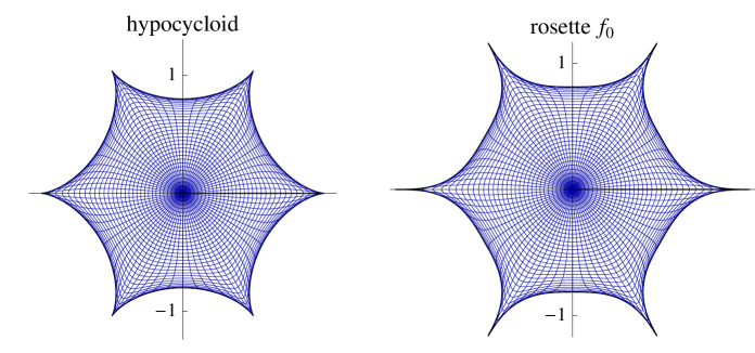
Figure 1. Images of a regular polar grid in $U$ under the 6-cusped hypocycloid (left) and a 6-cusped rosette mapping (right) defined by $f_{0}\left(z\right)=z\,_{2}F_{1}\left(\frac{1}{2},\frac{1}{12};\frac{13}{12};z^{12}\right)+\frac{1}{5}\bar{z}^{5}\,\overline{{}_{2}F_{1}\left(\frac{1}{2},\frac{5}{12};\frac{17}{12};z^{12}\right)}$

The rosette harmonic mappings introduced here can be viewed as modifications of the hypocycloid mappings, and are formulated by incorporating Gauss hypergeometric ${}_{2}F_{1}\,\$factors into the analytic and co-analytic parts. The rosette mappings $f_{\beta}$ will be defined in Section 3, but an example of a 6-cusped rosette mapping appears on the right of Figure 1. In comparison with the 6-cusped hypocycloid, the rosette has cusps that are more “pointy”. Figure 4 indicates further examples of rosette mappings for $n=6$ in which the images of the unit disk may have rotational but not reflectional symmetry.

The process by which we obtain rosette harmonic mappings with essentially different features, is by rotating the analytic and co-analytic parts relative to one another. In one interesting configuration, the analytic and co-analytic derivatives in the boundary extension alternate between “alignment” and “cancellation” on sub-arcs of $\partial U,$ leading to arcs of constancy on the boundary of the unit disk. Other harmonic mappings with arcs of constancy on the disk boundary are the Poisson extensions of piecewise constant functions defined on the unit circle; these mappings have been studied in [SS89], [DMS05], [McD12], and [BLW15], for instance.

In the forthcoming article [AM21], we explore the rosette minimal surfaces that “lift” from the rosette harmonic mappings. The hypocyloid mappings of Example 1.1 can lift to an Enneper surface. However the minimal graphs lifting from rosette harmonic mappings with the arcs of constancy described above, have interesting similarities and contrasts when compared with the Jenkins-Serrin surfaces. Jenkins-Serrin minimal surfaces arise as “lifts” of Poisson extensions of piecewise constant boundary functions - the same mappings referenced in the previous paragraph. The prototype for a Jenkins-Serrin surface is Schwarz’s first surface (see [Sch72]) which lifts from a harmonic mapping onto a square; more general Jenkins-Serrin surfaces are described in [JS66], and assume values of either $+\infty$ or $-\infty$ over the boundary segments connecting the vertices of the underlying harmonic mappings. Further Jenkins-Serrin surfaces have been explored in [DT00], and [MS08], for example. The rosette minimal graphs turn out to have in common with Jenkins-Serrin surfaces that the height function has a constant magnitude over the curves/straightedges connecting the vertices of the underlying harmonic mapping, and the completion of the minimal graphs contain vertical lines (these lines occur where the height function changes between a positive and negative value). These rosette minimal surfaces differ from the Jenkins-Serrin surfaces in that the constant values of the height function are finite.

It would be interesting to know further examples of harmonic mappings on the unit disk for which the boundary extensions have arcs of constancy mapping onto vertices, for which the boundary correspondence is continuous, and for which there exists a minimal surface lift with a piecewise constant height function over the boundary of the harmonic mapping.

The sections following this introduction are organized as follows: In Section 2, the properties of the ${}_{2}F_{1}$ hypergeometric functions utilized in the definition of the rosette harmonic mappings are described. In Section 3, the rosette harmonic mappings are defined and their rotational and reflectional symmetries are explored. In Section 4 we describe the boundary, that is piecewise smooth between the nodes and cusps that together form the image of the unit circle. In particular, we highlight the remarkable situation in which the rosette harmonic mapping is constant on alternating arcs that partition the unit circle. In Section 5 we use the argument principle for harmonic functions to show that the rosette harmonic mappings are in fact univalent. We also describe a computationally efficient way to construct the image of the unit disk by using rotations of a smaller “fundamental set”.

2. Hypergeometric functions

We begin by defining two Gauss hypergeometric ${}_{2}F_{1}$ functions.

Definition 2.1.

Let $U$ denote the unit disk. For $n\geq 2$ and $z\in\bar{U},$ consider the Gauss ${}_{2}F_{1}$ hypergeometric functions

$$H_{n}\left(z\right) =\,_{2}F_{1}\left(\frac{1}{2},\frac{1}{2n},1+\frac{1}{2n},z\right)$$

$$G_{n}\left(z\right) =\,_{2}F_{1}\left(\frac{1}{2},\frac{1}{2}-\frac{1}{2n},\frac{3}{2}-\frac{1}{2n},z\right)$$

for $n\geq 2.$ Note when $n=2$, that $G_{2}=H_{2}$.

By the Corollary in [MS61], $H_{n}$ and $G_{n}$ map the unit disk onto a convex region. Since $H_{n}\left(0\right)=G_{n}\left(0\right)=1,$ the convex regions $H_{n}\left(U\right)$ and $G_{n}\left(U\right)$ contain $1$. Thus $H_{n}$ and $G_{n}$ can be considered to be perturbations of the constant function of unit value. In Figure 2 where $n=6$, one can see the distortion from unity in $H_{6}\left(z\right)$ and $G_{6}\left(z\right).$ The reflectional symmetry in the real axis is also apparent. These and further properties of the hypergeometric functions $H_{n}$ and $G_{n}$ are stated in Proposition 2.2.

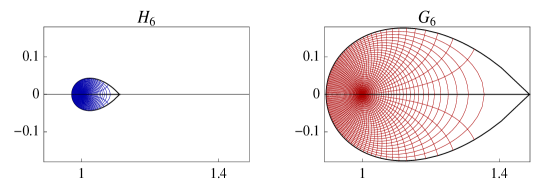
Figure 2. Images of a polar grid in $U$ under $H_{6}$ and $G_{6}.$

Proposition 2.2.

Let $n\geq 3.$
(i) The Taylor coefficients $c_{m}$ of $H_{n}\left(z\right)\,$and $d_{m}$ of $G_{n}\left(z\right)$ are given by the formulae

$$c_{m}=A_{m}\frac{1}{2mn+1}\text{ and }d_{m}=A_{m}\frac{n-1}{n\left(2m+1\right)-1},\text{ }m\geq 0,$$

where $A_{0}=1,$ and $A_{m}=\left(\begin{array}[c]{c}2m-1\\ m-1\end{array}\right)/2^{2m-1},$ for $m\geq 1.$
(ii) The hypergeometric functions $H_{n}$ and $G_{n}$ have reflectional symmetry

$$H_{n}\left(\bar{z}\right)=\overline{H_{n}\left(z\right)}\text{ and }G_{n}\left(\bar{z}\right)=\overline{G_{n}\left(z\right)}.$$

(iii) Both $H_{n}\$and $G_{n}$ are univalent mappings of the open unit disk onto a bounded convex region in the right half plane. Moreover, both series converge absolutely on the closed unit disk.
(iv) Define $K_{n}=H_{n}\left(1\right)$. Both $H_{n}\$and $G_{n}$ are positive for $x\in\left[-1,1\right],$ with the interval $\left[H_{n}\left(-1\right),H_{n}\left(1\right)\right]$ strictly contained in $\left[G_{n}\left(-1\right),G_{n}\left(1\right)\right],$ and the values at $1$ are as follows:

(2.1) $$H_{n}\left(1\right) =K_{n}=\sqrt{\pi}\frac{\Gamma\left(1+\frac{1}{2n}\right)}{\Gamma\left(\frac{1}{2}+\frac{1}{2n}\right)},$$

$$G_{n}\left(1\right) =\left(n-1\right)\tan\left(\frac{\pi}{2n}\right)K_{n}=\sqrt{\pi}\frac{\Gamma\left(\frac{3}{2}-\frac{1}{2n}\right)}{\Gamma\left(1-\frac{1}{2n}\right)}.$$

Moreover,

$$5/6<G_{n}\left(-1\right)<H_{n}\left(-1\right)<1<H_{n}\left(1\right)<G_{n}\left(1\right)<2.$$

Proof.

We first note the form of the Taylor coefficients $c_{m}$ of $H_{n},$ and $d_{m}$ of $G_{n},$ where $n\geq 2,$ and $m\geq 0.$ By the definition of hypergeometric series, and using the Pochhammer rising factorial symbol, we obtain

$$c_{m}=\frac{\left(\frac{1}{2}\right)_{m}\left(\frac{1}{2n}\right)_{m}}{m!\left(1+\frac{1}{2n}\right)_{m}}=A_{m}\frac{\left(\frac{1}{2n}\right)\left(\frac{1}{2n}+1\right)\left(\frac{1}{2n}+2\right)\ldots\left(\frac{1}{2n}+m-1\right)}{\left(\frac{1}{2n}+1\right)\left(\frac{1}{2n}+2\right)\ldots\left(\frac{1}{2n}+m-1\right)\left(\frac{1}{2n}+m\right)}$$

where we define $A_{m}=\left(\frac{1}{2}\right)_{m}/m!$ . All but two factors cancel, leaving

$$c_{m}=A_{m}\frac{\left(\frac{1}{2n}\right)}{\left(\frac{1}{2n}+m\right)}=A_{m}\frac{1}{2mn+1}.$$

A more familiar formula for $A_{m}$ in terms of binomial coefficients is obtained from

$$A_{m}=\frac{1\cdot 3\cdot 5\ldots\left(2m-1\right)}{2^{m}m!}=\frac{\left(2m-1\right)!}{\left(m-1\right)!2^{m-1}2^{m}m!}=\left(\begin{array}[c]{c}2m-1\\ m-1\end{array}\right)/2^{2m-1}.$$

The mth Taylor coefficient of $G_{n}$ is

$$d_{m}=\frac{\left(\frac{1}{2}\right)_{m}\left(\frac{1}{2}-\frac{1}{2n}\right)_{m}}{m!\left(\frac{3}{2}-\frac{1}{2n}\right)_{m}}=A_{m}\frac{\left(\frac{1}{2}-\frac{1}{2n}\right)_{m}}{\left(\frac{3}{2}-\frac{1}{2n}\right)_{m}}.$$

Again, upon expanding the Pochhammer symbols and simplifying we obtain

$$d_{m}=A_{m}\frac{\left(\frac{1}{2}-\frac{1}{2n}\right)}{\left(\frac{2m+1}{2}-\frac{1}{2n}\right)}=A_{m}\frac{n-1}{n\left(2m+1\right)-1},$$

establishing (i). Clearly these are positive term series, so the stated symmetries involving conjugation in (ii) hold. We now prove (iv). Because the coefficients $c_{m}$ and $d_{m}$ are positive for all $m=0,1,2,...,$ the real line maps to the real line under both $H_{n}$ and $G_{n}.$ Moreover, for $x>0$ the function values are positive, and increasing with $x$. Clearly $H_{n}\left(1\right)>1>H_{n}\left(-1\right),$ because the $c_{m}$ are positive with $c_{0}=1,$ and for $x<0,$ we obtain an alternating series. For $G_{n},$ we see that $d_{0}-d_{1}<G_{n}\left(-1\right)<d_{0}-d_{1}+d_{2}.$ Computing the lower bound, we obtain $d_{0}=1,$ and $d_{1}=A_{1}\frac{1}{2n+1}=\frac{1}{4n+2},$ so

$$G_{n}\left(-1\right)>d_{0}-d_{1}=1-\frac{1}{2}\frac{n-1}{3n-1}>1-\frac{1}{6}=5/6.$$

To see that $G_{n}\left(-1\right)<H_{n}\left(-1\right),$ we again use the alternating series test and show that the lower bound $c_{0}-c_{1}$ for $H_{n}\left(-1\right)$ is larger than the upper bound $d_{0}-d_{1}+d_{2}$ for $G_{n}\left(-1\right).$ We show that the equivalent inequality $c_{1}+d_{2}\leq d_{1}$ holds. Note that $A_{1}=\frac{1}{2}$ and $A_{2}=\frac{3}{8},$ so the inequality becomes

$$\frac{1}{2}\frac{1}{2n+1}+\frac{3}{8}\frac{n-1}{5n-1}\leq\frac{1}{2}\frac{n-1}{3n-1}$$

which after some algebra is equivalent to $\left(n-3\right)\left(22n^{2}-7n+1\right)\geq 0.$ The latter is true for $n\geq 3,$ with equality at $n=3.$ Thus the inequalities $G_{n}\left(-1\right)<H_{n}\left(-1\right)<1$ hold for $n\geq 3$. Finally, coefficient by coefficient, the following equivalent inequalities are equivalent to $c_{m}<d_{m}$ for $m=1,2,3,...$

$$A_{m}\frac{1}{2mn+1} <A_{m}\frac{n-1}{n\left(2m+1\right)-1}$$

$$0 <2mn\left(n-2\right),$$

and this last inequality is clearly true for all $m=1,2,...$ when $n>2$. Thus $H_{n}\left(1\right)<G_{n}\left(1\right).$ Finally we use Theorem 18 in §32  of [Rai71] to compute

$$K_{n}=H_{n}\left(1\right)=\sqrt{\pi}\frac{\Gamma\left(1+\frac{1}{2n}\right)}{\Gamma\left(\frac{1}{2}+\frac{1}{2n}\right)}\text{ and }G_{n}\left(1\right)=\sqrt{\pi}\frac{\Gamma\left(\frac{3}{2}-\frac{1}{2n}\right)}{\Gamma\left(1-\frac{1}{2n}\right)}$$

Note that

$$G_{n}\left(1\right)/H_{n}\left(1\right)=\frac{\Gamma\left(\frac{3}{2}-\frac{1}{2n}\right)}{\Gamma\left(1-\frac{1}{2n}\right)}\frac{\Gamma\left(\frac{1}{2}+\frac{1}{2n}\right)}{\Gamma\left(1+\frac{1}{2n}\right)}=\frac{\Gamma\left(\frac{1}{2}+\frac{1}{2n}\right)\Gamma\left(\frac{3}{2}-\frac{1}{2n}\right)}{\Gamma\left(1+\frac{1}{2n}\right)\Gamma\left(1-\frac{1}{2n}\right)}.$$

From the well known identities for the gamma function, $\Gamma\left(z+1\right)=z\Gamma\left(z\right),$ and $\Gamma\left(z\right)\Gamma\left(1-z\right)=\pi/\sin\left(\pi z\right),$ we obtain

$$\Gamma\left(1+z\right)\Gamma\left(1-z\right)=\left(\pi z\right)/\sin\left(\pi z\right).$$

Therefore

$$G_{n}\left(1\right)/H_{n}\left(1\right)=\frac{\pi\left(\frac{1}{2}-\frac{1}{2n}\right)}{\sin\left(\pi\left(\frac{1}{2}-\frac{1}{2n}\right)\right)}\frac{\sin\left(\pi\frac{1}{2n}\right)}{\pi\frac{1}{2n}}=\left(n-1\right)\frac{\sin\left(\pi/2n\right)}{\cos\left(\pi/2n\right)}=\left(n-1\right)\tan\left(\pi/2n\right).$$

We finish by proving (iii). The radius of convergence of any Gauss hypergeometric series is 1. However the convergence on the closed disk is guaranteed for ${}_{2}F_{1}\left(a,b,c,z\right)$ whenever $\operatorname{Re}\left(c-a-b\right)>0$ (Section 29 of [Rai71]); here $\operatorname{Re}\left(c-a-b\right)=1/2\,\,$for both $G_{n}$ and $H_{n}$. Because both $G_{n}$ and $H_{n}$ satisfy (ii) of the Corollary in [MS61], ${}_{2}F_{1}\left(a,b,c,z\right)$ maps the open disk univalently onto a convex region. Because of positive Taylor coefficients, we have $G_{n}\left(-1\right)<\operatorname{Re}G_{n}\left(z\right)<G_{n}\left(1\right)$ and $H_{n}\left(-1\right)<\operatorname{Re}H_{n}\left(z\right)<H_{n}\left(1\right).$ Thus the images $H_{n}\left(U\right)$ and $G_{n}\left(U\right)$ are convex sets within the lines $\operatorname{Re}z=5/6$ and $\operatorname{Re}z=2.$ ∎

Examples of the hypergeometric functions $H_{n}$ and $G_{n}$ are calculated in [AM21], through applying the shear construction of [CSS84] to a particular conformal mapping onto a regular 12-gon. This shear was in fact the origin of the first rosette mapping. The functions $H_{n}$ and $G_{n}$ appear in antiderivatives associated with several related radical expressions in [AM21], and are restated here.

Proposition 2.3.

Let $n\geq 2,\,$and let $z\in U.$ Then

(2.2) $$\int_{0}^{z}\frac{1}{\sqrt{1-\zeta^{2n}}}d\zeta =zH_{n}\left(z^{2n}\right)$$

(2.3) $$\int_{0}^{z}\frac{\zeta^{n-2}}{\sqrt{1-\zeta^{2n}}}d\zeta =\frac{z^{n-1}}{n-1}G_{n}\left(z^{2n}\right).$$

Proof.

The integrations are carried out using the Gauss hypergeometric formula, as indicated in [AM21]. The integrals are restated here in terms of the notation introduced in Definition 2.1. ∎

3. Rosette Harmonic Mappings

The analytic antiderivatives of Proposition 2.3 are defined below as $h_{n}\left(z\right)$ and $g_{n}\left(z\right).$ These become (rotations aside) the analytic and co-analytic parts of the rosette harmonic mappings in Definition 3.5. We note the similarity with the analytic and co-analytic parts of the hypocycloid, modified here with hypergeometric factors.

Definition 3.1.

For $n\geq 2$ and $n\in\mathbb{N}$, define the analytic functions

$$h_{n}\left(z\right)=z\,H_{n}\left(z^{2n}\right),\text{ \ }g_{n}\left(z\right)=\frac{z^{n-1}}{n-1}G_{n}\left(z^{2n}\right),\text{ }z\in\bar{U}$$

where $H_{n}$ and $G_{n}$ are the hypergeometric ${}_{2}F_{1}$ functions of Definition 2.1.

Remark 3.2.

In the current context, we consider only $n\geq 3$ for rosette harmonic mappings, but we note that when $n=2,$ $h_{n}\left(z\right)=g_{n}\left(z\right)$ becomes the standard Schwarz-Christoffel mapping of the unit disk onto a square.

The function $h_{n}$ can easily be shown to be starlike and therefore univalent on the unit disk. However $g_{n}$ is not univalent for $n\geq 3$. The image $h_{6}\left(\bar{U}\right)$ is shown on the left of Figure 3, and a portion of the graph of $\overline{g_{6}}\left(\bar{U}\right)$ is shown on the right, with $z$ restricted to $\left\{z\in\bar{U}:\arg z\in\left(0,\left(5/2\right)\pi/n\right)\right\}$.

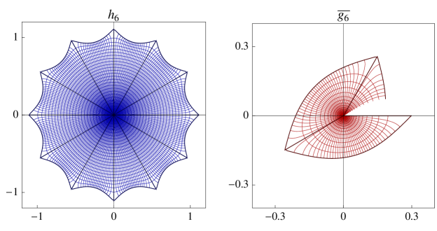
Figure 3. Image of $\bar{U}$ under $h_{6}$ (left), and a first-quadrant sector of $\bar{U}$ under $\overline{g_{6}}$ (right). Note that the image of $\overline{g_{6}}$ is relatively enlarged.

Proposition 3.3.

Let $n\geq 3$ and let $\zeta$ be a primitive $2nth$ root of unity. Then $h_{n}\left(z\right)$ and $g_{n}\left(z\right)$ are continuous on $\bar{U}$ and analytic on $\overline{U}\backslash\left\{\zeta^{j}:j=1,2,...,2n\right\}.$ Additionally the following hold.
(i) Reflectional symmetries $h_{n}\left(\bar{z}\right)=\overline{h_{n}\left(z\right)}$ and $g_{n}\left(\bar{z}\right)=\overline{g_{n}\left(z\right)}$ are present.
(ii) The functions $h_{n}\left(e^{it}\right)$ and $g_{n}\left(e^{it}\right)$ have magnitudes $\left|H_{n}\left(e^{i2nt}\right)\right|$ and
$\frac{1}{n-1}\left|G_{n}\left(e^{i2nt}\right)\right|,$ and these magnitudes are each $\left(\pi/n\right)$-periodic as functions of $t.$ Moreover, convergence at $H\left(1\right)$ and $G\left(1\right)$ is not uniform.
(iii) Both $h_{n}$ and $g_{n}$ exhibit $2n$-fold rotational symmetry: for  $j\in\mathbb{Z},$

(3.1) $$h_{n}\left(e^{ij\pi/n}z\right)=e^{ij\pi/n}h_{n}\left(z\right)\text{ and }g_{n}\left(e^{ij\pi/n}z\right)=\left(-1\right)^{j}e^{-ij\pi/n}g_{n}\left(z\right).$$

(iv) The derivatives of $h_{n}\left(z\right)$ and $g_{n}\left(z\right)$ are given by

(3.2) $$h_{n}^{\prime}\left(z\right)=\frac{1}{\sqrt{1-z^{2n}}}\text{ and }g_{n}^{\prime}\left(z\right)=\frac{z^{n-2}}{\sqrt{1-z^{2n}}}.$$

Proof.

The stated symmetries in (i) follow from the reflections $H_{n}\left(\bar{z}^{2n}\right)=\overline{H_{n}\left(z^{2n}\right)}$ and $G_{n}\left(\bar{z}^{2n}\right)=\overline{G_{n}\left(z^{2n}\right)}$ of Proposition 2.2 (ii). For (ii) we easily compute $\left|h_{n}\left(e^{it}\right)\right|=\left|e^{it}H_{n}\left(e^{i2nt}\right)\right|$ and $\left|g_{n}\left(e^{it}\right)\right|=\left|e^{i\left(n-1\right)t}G_{n}\left(e^{i2nt}\right)\right|/\left(n-1\right)$ to see that $h_{n}\left(e^{it}\right)$ and $g_{n}\left(e^{it}\right)$ have the stated magnitudes. These magnitudes have period $\pi/n$ as functions of $t,$ since each of $H_{n}\left(e^{it}\right)$ and $G_{n}\left(e^{it}\right)$ have period $2\pi$ as functions of $t.$ For (iii), first note that $\left(e^{ij\pi/n}z\right)^{2n}=z^{2n}$ and $\left(e^{ij\pi/n}\right)^{n-1}=e^{ij\pi}e^{-ij\pi/n}=\left(-1\right)^{j}e^{-ij\pi/n}$ for any integer $j.$ Thus

$$h_{n}\left(e^{ij\pi/n}z\right)=e^{ij\pi/n}zH_{n}\left(\left(e^{ij\pi/n}z\right)^{2n}\right)=e^{ij\pi/n}h_{n}\left(z\right),\text{ and}$$

$$g_{n}\left(e^{ij\pi/n}z\right)=\frac{1}{n-1}\left(e^{ij\pi/n}z\right)^{n-1}G_{n}\left(\left(e^{ij\pi/n}z\right)^{2n}\right)=e^{ij\left(\pi-\pi/n\right)}g_{n}\left(z\right).$$

For (iv), the derivatives are immediate from (2.2) and (2.3). The stated region of analyticity of the functions $h_{n}$ and $g_{n}$ is due to the fact that their derivatives can be analytically continued across the boundary, except at the 2nth roots of unity where derivatives do not exist. Moreover the convergence of $H\left(1\right)$ and $G\left(1\right)$ is not uniform, since this would imply analyticity at $\zeta$. ∎

Corollary 3.4.

Let $z=re^{ij\pi/n},$ and $j\in\mathbb{Z}.$ Then

$$h_{n}\left(re^{ij\pi/n}\right)=e^{ij\pi/n}h_{n}\left(r\right)\text{ and }\overline{g_{n}\left(re^{ij\pi/n}\right)}=\left(-1\right)^{j}e^{ij\pi/n}g_{n}\left(r\right)$$

and on these rays, $\arg\left(h_{n}\left(z\right)\right)=\arg z,$ and $\arg\left(\overline{g_{n}\left(z\right)}\right)=\arg\left(\frac{1}{n-1}\bar{z}^{n-1}\right).$

Proof.

By Proposition 2.2 (iv), $H_{n}$ and $G_{n}$ map reals to positive reals. Thus $h_{n}$ and $g_{n}$ map positive reals to positive reals. Now let $z=re^{ij\pi/n}$ for $r>0$ in formula (3.1). ∎

We now define the rosette harmonic mappings.

Definition 3.5.

Let $n\in\mathbb{N}$ with $n\geq 3,$ and let $h_{n}$ and $g_{n}$ be defined as in Definition 3.1. For each $\beta\in\mathbb{R},$ define the rosette harmonic mapping

$$f_{\beta}\left(z\right)=e^{i\beta/2}h_{n}\left(z\right)+e^{-i\beta/2}\overline{g_{n}\left(z\right)},\text{ }z\in\bar{U}.$$

Then $f_{\beta}\left(z\right)$ is harmonic on $U,$ and continuous on $\bar{U}.$ Denote the dilatation of $f_{\beta}\left(z\right)$ by $\omega\left(z\right)$ on $\bar{U}\backslash\left\{\zeta^{j}:j=1,2,...,2n\right\},$ where $\zeta$ is a primitive 2nth root of unity.

Remark 3.6.

For simplicity of the notation, we do not notate the value of $n,$ which is apparent from context, and fixed as a constant in our discussions. The dilatation is independent of $\beta$ and we simplify our notation to $\omega$ instead of using $\omega_{f_{\beta}}.$

The derivatives of the analytic and co-analytic parts (for $\beta=0$) in equation (3.2) are the same as the corresponding derivatives for the hypocycloid, except for the radical factor. This factor affects the argument of the summands in the canonical decomposition, but Corollary 3.4 shows that along rays $\left\{re^{ij\pi/n}:r>0\right\}$ where $j\in\mathbb{Z},$ that $h_{n}$ and $\overline{g_{n}}$ are collinear. Moreover Corollary 3.4 shows that on these same rays, that $h_{n}$ and $\bar{g}_{n}$ have the same arguments as their analytic and anti-analytic counterparts in the hypocycloid mapping. Thus $f_{0}\left(z\right)$ and $f_{hyp}\left(z\right)$ are collinear along these radial lines (as indicated in Figure 1). Figure 4 shows images $f_{\beta}\left(U\right)$ as $\beta$ varies, and suggests that different harmonic mappings $f_{\beta}$ are obtained for the four different values of $\beta$ there. This contrasts with the hypocycloid mapping, where rotating the analytic and anti-analytic parts $z$ and $\frac{1}{n-1}\bar{z}^{n-1}$ relative to one another does not yield a graph that is essentially different.

One may ask what other maps could be obtained through adding different rotations of $h_{n}$ and $\overline{g_{n}}$. The next proposition shows that if we consider arbitrary rotations of the analytic and co-analytic parts, by $\theta$ and $\tilde{\theta}$ say, then the result will in fact be a rotation of a rosette harmonic mapping.

Proposition 3.7.

Let $\theta$ and $\tilde{\theta}$ be arbitrary real angles. Then $e^{i\theta}h_{n}\left(z\right)+\overline{e^{i\tilde{\theta}}g_{n}\left(z\right)}$ is a rotation $e^{i\gamma}f_{\beta}$ for some real angles $\gamma$ and $\beta.$

Proof.

Note that the harmonic function $e^{i\theta}h_{n}\left(z\right)+\overline{e^{i\tilde{\theta}}g_{n}\left(z\right)}$ can be rewritten

$$e^{-i\tilde{\theta}}\left(e^{i\theta}e^{i\tilde{\theta}}h_{n}\left(z\right)+\overline{g_{n}\left(z\right)}\right)$$

$$=e^{-i\tilde{\theta}}e^{i\left(\theta+\tilde{\theta}\right)/2}\left(e^{i\left(\theta+\tilde{\theta}\right)/2}h_{n}\left(z\right)+e^{-i\left(\theta+\tilde{\theta}\right)/2}\overline{g_{n}\left(z\right)}\right)$$

$$=e^{i\left(\theta-\tilde{\theta}\right)/2}f_{\theta+\tilde{\theta}}\left(z\right)$$

Thus $e^{i\theta}h_{n}\left(z\right)+\overline{e^{i\tilde{\theta}}g_{n}\left(z\right)}$ can be obtained by a rotation by $\gamma=\left(\theta-\tilde{\theta}\right)/2$ of the map $f_{\beta}$ where $\beta=\theta+\tilde{\theta}.$ ∎

Thus the family of mappings $\left\{f_{\beta}:\beta\in\mathbb{R}\right\}$ represents all of the different mappings, up to rotation, that arise from arbitrary rotations of $h_{n}$ and $g_{n}$. We show in Proposition 3.8 that $f_{\beta+\pi}$ is essentially the same mapping as $f_{\beta}.$

Proposition 3.8.

(i) For any  $\beta\in\mathbb{R},$ the functions $f_{\beta}$ and $f_{\beta+\pi}$ are related by

(3.3) $$f_{\beta}\left(z\right)=e^{-i\left(\frac{\pi}{2}+\frac{\pi}{n}\right)}f_{\beta+\pi}\left(e^{i\frac{\pi}{n}}z\right).$$

Thus the image $f_{\beta+\pi}\left(U\right)$ is equal to a rotation of the image $f_{\beta}\left(U\right)$.
(ii) If $\beta<0,$ then the image of any point under $f_{\beta}$ is a reflection in the real axis of the same point under $f_{-\beta},$ where $-\beta>0.$  Specifically, $f_{\beta}\left(\bar{z}\right)=\overline{f_{-\beta}\left(z\right)}.$

Proof.

(i) We compute, using $j=1$ in equation (3.1),

$$f_{\pi+\beta}\left(e^{i\frac{\pi}{n}}z\right)=e^{i\left(\pi/2+\beta/2\right)}e^{i\pi/n}h_{n}\left(z\right)+e^{-i\left(\pi/2+\beta/2\right)}\overline{\left(-1\right)e^{-i\pi/n}g_{n}\left(z\right)}.$$

Multiplying by $e^{-i\left(\frac{\pi}{2}+\frac{\pi}{n}\right)},$ and noting that $-e^{-i\frac{\pi}{2}}=e^{i\frac{\pi}{2}},$

$$e^{-i\left(\frac{\pi}{2}+\frac{\pi}{n}\right)}f_{\pi+\beta}\left(e^{i\frac{\pi}{n}}z\right)=e^{i\beta/2}h_{n}\left(z\right)+e^{-i\beta/2}g_{n}\left(z\right)=f_{\beta}\left(z\right).$$

(ii) Once again, by computation:

$$f_{\beta}\left(\bar{z}\right)=e^{i\frac{\beta}{2}}h_{n}\left(\bar{z}\right)+e^{-i\frac{\beta}{2}}\overline{g_{n}\left(\bar{z}\right)}=e^{i\frac{\beta}{2}}\overline{h_{n}\left(z\right)}+e^{-i\frac{\beta}{2}}g_{n}\left(z\right)$$

while

$$f_{-\beta}\left(z\right)=e^{-i\frac{\beta}{2}}h_{n}\left(z\right)+e^{i\frac{\beta}{2}}\overline{g_{n}\left(z\right)}.$$

The last two expressions are conjugates of one another. $\blacksquare$ ∎

Corollary 3.9.

Let $\tilde{\beta}\in\mathbb{R},$ and let $\tilde{\beta}=\beta+l\pi$ for some $l\in\mathbb{Z}.$ Then

(3.4) $$f_{\beta+l\pi}\left(z\right)=e^{il\left(\pi/n+\pi/2\right)}f_{\beta}\left(e^{-il\pi/n}z\right).$$

Proof.

Solving equation (3.3) we have $f_{\beta+\pi}\left(z\right)=e^{i\left(\pi/2+\pi/n\right)}f_{\beta}\left(e^{-i\pi/n}z\right).$ Equation (3.4) is obtained by repeated application of this equation. ∎

Proposition 3.8 (i) shows that up to rotations (pre and post composed), all rosette mappings are represented in the set $\left\{f_{\beta}:\beta\in(-\pi/2,\pi/2]\right\}.$ We will see in Section 4 that these rosette mappings are all distinct from one another in that no rosette mapping in the set can be obtained by rotations from another. Proposition 3.8 (ii) allows us to consider just $\left\{f_{\beta}:\beta\in\left[0,\pi/2\right]\right\}$ to obtain all rosette mappings, up to rotation and reflection.

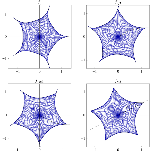
Figure 4. Images of $U$ under $f_{\beta}$ with $n=5.$ The darker ”radial curve” indicates the image of $\left[0,1\right].$ The graphs $f_{\pi/3}$ and $f_{-\pi/3}$ illustrate Proposition 3.8 (ii). The images $f_{-\pi/3}\left(U\right)$ and $f_{\pi/3}\left(U\right)$ have cyclic symmetry while $f_{0}\left(U\right)$ and $f_{\pi/2}\left(U\right)$ exhibit dihedral symmetry, illustrating Theorem 3.10. For $f_{\pi/2}$ the line of symmetry $\arg z=\pi/4-\pi/\left(2n\right)$ is indicated.

Figure 4 illustrates that $f_{-\pi/3}\left(U\right)$ and $f_{\pi/3}\left(U\right)$ are reflections of one another. The example graphs in Figure 4 also demonstrate the rotational and reflectional symmetries apparent within any particular graph $f_{\beta}\left(U\right),$ as stated in the following theorem.

Theorem 3.10.

Let $n\in\mathbb{N}$ and $n\geq 3.$
(i) The harmonic functions $f_{\beta}\left(z\right)$, $\beta\in\mathbb{R}$ have dilatation $\omega\left(z\right)=z^{n-2}$ for $z\in U.$
(ii) The rosette mapping $f_{\beta}\left(z\right)$, $\beta\in\mathbb{R}$ has n-fold rotational symmetry, that is

(3.5) $$f_{\beta}\left(e^{i2k\pi/n}z\right)=e^{i2k\pi/n}f_{\beta}\left(z\right),\text{ where }z\in\bar{U},\text{ }k\in\mathbb{Z}.$$

(iii) If $\beta$ is an integer multiple of $\pi/2,$ then the image $f_{\beta}\left(U\right)$ has reflectional symmetry. For $\beta=0$ and $\beta=\pi/2$ the reflections are

(3.6) $$f_{0}\left(\overline{z}\right)=\overline{f_{0}\left(z\right)}\text{ and }e^{i\eta}f_{\pi/2}\left(e^{i\gamma}\overline{z}\right)=\overline{e^{i\eta}f_{\pi/2}\left(e^{i\gamma}z\right)},$$

where $\eta=\pi/\left(2n\right)-\pi/4$ and $\gamma=-\pi/\left(2n\right).$ Thus if $z$ and $z^{\prime}$ are reflections in $\arg z=\gamma,$ then $f_{\pi/2}\left(z\right)$ and $f_{\pi/2}\left(z^{\prime}\right)$ are reflections in $\arg z=\eta$.

Proof.

(i) We compute $\omega\left(z\right)=$ $g_{n}^{\prime}\left(z\right)/h_{n}^{\prime}\left(z\right)$ from the derivative expressions in (3.2), noting that the constant $e^{i\beta/2},$ and the radicals, cancel leaving $z^{n-2}.$
(ii) From equation (3.1) with $j=2k$ we have $h_{n}\left(e^{i2k\pi/n}z\right)=e^{i2k\pi/n}h_{n}\left(z\right)$ and $\overline{g_{n}\left(e^{i2k\pi/n}z\right)}=e^{i2k\pi/n}\overline{g_{n}\left(z\right)}$. Thus

$$f_{\beta}\left(e^{i2k\pi/n}z\right)=e^{i2k\pi/n}\left(e^{i\beta/2}h_{n}\left(z\right)+e^{-i\beta/2}\overline{g_{n}\left(z\right)}\right)=e^{i2k\pi/n}f_{\beta}\left(z\right)\text{.}$$

(iii) From Proposition 3.3, $f_{0}(\overline{z})=h_{n}(\bar{z})+\overline{g_{n}\left(\bar{z}\right)}=\overline{h_{n}(z)}+g_{n}\left(z\right)=\overline{f_{0}\left(z\right)}.$ For $f_{\pi/2},$ consider the expressions $f_{\pi/2}\left(e^{i\gamma}\overline{z}\right)$ and $f_{\pi/2}\left(e^{i\gamma}z\right)$:

$$f_{\pi/2}\left(e^{i\gamma}\overline{z}\right) =e^{i\pi/4}h_{n}\left(e^{-i\pi/\left(2n\right)}\bar{z}\right)+e^{-i\pi/4}\overline{g_{n}\left(e^{-i\pi/\left(2n\right)}\bar{z}\right)}$$

$$=e^{i\pi/4}\overline{h_{n}\left(e^{i\pi/\left(2n\right)}z\right)}+e^{-i\pi/4}g_{n}\left(e^{i\pi/\left(2n\right)}z\right)$$

$$=e^{i\pi/4}\overline{e^{i\pi/\left(2n\right)}zH\left(-z^{2n}\right)}+e^{-i\pi/4}ie^{-i\pi/\left(2n\right)}\frac{z^{n-1}G\left(-z^{2n}\right)}{n-1}$$

$$=e^{i\left(\pi/4-\pi/\left(2n\right)\right)}\left(\overline{zH\left(-z^{2n}\right)}+\frac{z^{n-1}G\left(-z^{2n}\right)}{n-1}\right).$$

Note that $\left(e^{i\pi/\left(2n\right)}\right)^{n-1}=ie^{-i\pi/\left(2n\right)}$ and $\left(e^{-i\pi/\left(2n\right)}z\right)^{2n}=-z^{2n},$ as used in the calculation above. We also use $\left(e^{-i\pi/\left(2n\right)}\right)^{n-1}=-ie^{i\pi/\left(2n\right)}\$below:

$$f_{\pi/2}\left(e^{i\gamma}z\right) =e^{i\pi/4}h_{n}\left(e^{-i\frac{\pi}{2n}}z\right)+e^{-i\pi/4}\overline{g_{n}\left(e^{-i\frac{\pi}{2n}}z\right)}$$

$$=e^{i\pi/4}\left(e^{-i\frac{\pi}{2n}}z\right)H\left(e^{-i\pi}z^{2n}\right)+e^{-i\pi/4}\overline{\left(-i\right)e^{i\frac{\pi}{2n}}\frac{z^{n-1}}{n-1}G\left(-z^{2n}\right)}$$

$$=e^{i\left(\pi/4-\pi/\left(2n\right)\right)}\left(zH\left(-z^{2n}\right)+\overline{\frac{z^{n-1}}{n-1}G\left(-z^{2n}\right)}\right).$$

Multiplying each of $f_{\pi/2}\left(e^{i\gamma}\overline{z}\right)$ and $f_{\pi/2}\left(e^{i\gamma}z\right)$ by $e^{i\eta}=e^{i\left(\pi/4-\pi/\left(2n\right)\right)},$ we see that $e^{i\eta}$ $f_{\pi/2}\left(e^{i\gamma}\overline{z}\right)$ and $e^{i\eta}f_{\pi/2}\left(e^{i\gamma}z\right)$ are conjugates of one another.   Thus the stated equations in (iii) hold. ∎

In Section 4 we use features of the boundary $\partial f_{\beta}\left(U\right)$ that allow us to demonstrate the precise symmetry group for each graph $f_{\beta}\left(U\right)$, $\beta\in\mathbb{R}$ (see Corollary 4.14). Theorem 3.10 also shows that for a given $n\geq 3$ the rosette mappings $f_{\beta}$ and $n$-cusped hypocycloid all have the same dilatation. The equal dilatations result in similarities in the tangents of the rosette and hypocycloid boundary curves, to be discussed further in Section 4.

We finish this section by laying out geometric features that are specific to rosette mappings for $\beta$ in the interval $\beta\in(-\pi/2,\pi/2].$ These facts in combination with equation (3.4) will allow us to extend our conclusions for any $\beta\in\mathbb{R}.$

Lemma 3.11.

Let $n\in\mathbb{N},$ $n\geq 3,$ and recall $K_{n}=\sqrt{\pi}\,\Gamma\left(1+\frac{1}{2n}\right)/\Gamma\left(\frac{1}{2}+\frac{1}{2n}\right).$
(i) For $\beta\in(-\pi/2,\pi/2],$ we have polar forms for $f_{\beta}\left(1\right)$ and $f_{\beta}\left(e^{i\pi/n}\right)$ given by magnitudes $\left|f_{\beta}\left(1\right)\right|$ and $\left|f_{\beta}\left(e^{i\pi/n}\right)\right|$ which are, respectively,

(3.7) $$K_{n}\sqrt{\sec^{2}\left(\frac{\pi}{2n}\right)+2\tan\left(\frac{\pi}{2n}\right)\cos\beta}\text{ and }K_{n}\sqrt{\sec^{2}\left(\frac{\pi}{2n}\right)-2\tan\left(\frac{\pi}{2n}\right)\cos\beta},$$

and by the arguments $\psi=\arg\left(f_{\beta}\left(1\right)\right)$ and $\pi/n+\psi^{\prime}=\arg\left(f_{\beta}\left(e^{i\pi/n}\right)\right),$ where

(3.8) $$\tan\psi=\frac{1-\tan\left(\frac{\pi}{2n}\right)}{1+\tan\left(\frac{\pi}{2n}\right)}\tan\left(\frac{\beta}{2}\right)\text{ and }\tan\psi^{\prime}=\frac{1+\tan\left(\frac{\pi}{2n}\right)}{1-\tan\left(\frac{\pi}{2n}\right)}\tan\left(\frac{\beta}{2}\right).$$

If $\beta=0$ then both $\psi$ and $\psi^{\prime}$ are zero. If $\beta=\pi/2,$ these angles reduce to $\psi=\pi/4-\pi/\left(2n\right)$ and $\psi^{\prime}=\pi/4+\pi/\left(2n\right).$
(ii) If $\beta\in(0,\pi/2],$ then the curves $f_{\beta}\left(r\right)$ and $f_{\beta}\left(re^{i\pi/n}\right)$ have strictly increasing magnitude. Moreover, $\arg\frac{\partial}{\partial r}f_{\beta}\left(r\right)$ decreases strictly with $r$, and $\arg\frac{\partial}{\partial r}f_{\beta}\left(re^{i\pi/n}\right),$ increases strictly with $r$. We also have the following arguments for the the tangents of these curves at the origin

$$\lim_{r\rightarrow 0^{+}}\arg\frac{\partial}{\partial r}f_{\beta}\left(r\right)=\beta/2\text{ and }\lim_{r\rightarrow 0^{+}}\arg\frac{\partial}{\partial r}f_{\beta}\left(re^{i\pi/n}\right)=\beta/2+\pi/n,$$

and at the boundary of $U$

$$\lim_{r\rightarrow 1^{-}}\arg\frac{\partial}{\partial r}f_{\beta}\left(r\right)=0\text{ and }\lim_{r\rightarrow 1^{-}}\arg\frac{\partial}{\partial r}f_{\beta}\left(re^{i\pi/n}\right)=\pi/2+\pi/n.$$

(iii) For $\beta=0$ the curves $f_{0}\left(r\right)$ and $f_{0}\left(re^{i\pi/n}\right)$ are straight line-segments - the images have constant argument of $0$ and $\pi/n,$ respectively.

Proof.

To prove (i), we compute

$$f_{\beta}\left(r\right) =e^{i\beta/2}h_{n}\left(r\right)+e^{-i\beta/2}g_{n}\left(r\right)$$

$$=\cos\left(\beta/2\right)\left(h_{n}\left(r\right)+g_{n}\left(r\right)\right)+i\sin\left(\beta/2\right)\left(h_{n}\left(r\right)-g_{n}\left(r\right)\right),$$

and, upon recalling from Corollary 3.4 that $\overline{g_{n}\left(re^{i\pi/n}\right)}=e^{-i\pi/n}g_{n}\left(r\right),$

$$f_{\beta}\left(re^{i\pi/n}\right) =e^{i\beta/2}h_{n}\left(re^{i\pi/n}\right)+e^{-i\beta/2}\overline{e^{-i\pi/n}g_{n}\left(r\right)}$$

$$=e^{i\pi/n}\left(\cos\left(\beta/2\right)\left(h_{n}\left(r\right)-g_{n}\left(r\right)\right)+i\sin\left(\beta/2\right)\left(h_{n}\left(r\right)+g_{n}\left(r\right)\right)\right).$$

We recall the formulae $h_{n}\left(1\right)=H_{n}\left(1\right)=K_{n}$ and $g_{n}\left(1\right)=G_{n}\left(1\right)/\left(n-1\right)=\tan\left(\pi/\left(2n\right)\right)K_{n}$ from Proposition 2.2. Using continuity of $f_{\beta}$ on $\bar{U}$, we take limits as $r\rightarrow 1^{-}$ to get

$$f_{\beta}\left(1\right) =K_{n}\left(\cos\left(\beta/2\right)\left(1+\tan\left(\frac{\pi}{2n}\right)\right)+i\sin\left(\beta/2\right)\left(1-\tan\left(\frac{\pi}{2n}\right)\right)\right)\text{ and}$$

$$f_{\beta}\left(e^{i\pi/n}\right) =e^{i\pi/n}K_{n}\left(\cos\left(\beta/2\right)\left(1-\tan\left(\frac{\pi}{2n}\right)\right)+i\sin\left(\beta/2\right)\left(1+\tan\left(\frac{\pi}{2n}\right)\right)\right).$$

Moreover, writing $\psi=\arg f_{\beta}\left(1\right),$ and $\pi/n+\psi^{\prime}=\arg f_{\beta}\left(e^{i\pi/n}\right),$ we take ratios of imaginary to real parts of $f_{\beta}\left(1\right)$ and $f_{\beta}\left(e^{i\pi/n}\right)$ to easily obtain the stated formulae for $\tan\psi$ and $\tan\psi^{\prime}.$ We also readily obtain

$$\left|f_{\beta}\left(1\right)\right|^{2} =K_{n}^{2}\left(1+2\tan\left(\frac{\pi}{2n}\right)\cos\beta+\tan^{2}\left(\frac{\pi}{2n}\right)\right)\text{ and }$$

$$\left|f_{\beta}\left(e^{i\pi/n}\right)\right|^{2} =K_{n}^{2}\left(1-2\tan\left(\frac{\pi}{2n}\right)\cos\beta+\tan^{2}\left(\frac{\pi}{2n}\right)\right)$$

We can rewrite $1+\tan^{2}\left(\pi/\left(2n\right)\right)=\sec^{2}\left(\pi/\left(2n\right)\right)$ to obtain the magnitudes stated in (i). For (ii), taking derivatives of the formulae first derived for $f_{\beta}\left(r\right)$ and $f_{\beta}\left(re^{i\pi/n}\right),$ we obtain

$$\frac{\partial}{\partial r}f_{\beta}\left(r\right) =\cos\left(\beta/2\right)\left(\frac{1+r^{n-2}}{\sqrt{1-r^{2n}}}\right)+i\sin\left(\beta/2\right)\left(\frac{1-r^{n-2}}{\sqrt{1-r^{2n}}}\right)\text{ and }$$

$$\frac{\partial}{\partial r}f_{\beta}\left(re^{i\pi/n}\right) =e^{i\pi/n}\left(\cos\left(\beta/2\right)\left(\frac{1-r^{n-2}}{\sqrt{1-r^{2n}}}\right)+i\sin\left(\beta/2\right)\left(\frac{1+r^{n-2}}{\sqrt{1-r^{2n}}}\right)\right).$$

The arguments of these derivatives, namely $\arg\frac{\partial}{\partial r}f_{\beta}\left(r\right)$ and $\arg\frac{\partial}{\partial r}f_{\beta}\left(re^{i\pi/n}\right)$ are respectively

$$\arctan\left(\tan\left(\beta/2\right)\frac{1-r^{n-2}}{1+r^{n-2}}\right)\text{ and }\pi/n+\arctan\left(\tan\left(\beta/2\right)\frac{1+r^{n-2}}{1-r^{n-2}}\right),$$

whence the stated monotonicity of $\arg\frac{\partial}{\partial r}f_{\beta}\left(r\right)$ and $\arg\frac{\partial}{\partial r}f_{\beta}\left(re^{i\pi/n}\right)$ in (ii).The limits in (ii) are now easily computed. Note that as $r\rightarrow 1^{-},$ the ratio $\frac{1+r^{n-2}}{1-r^{n-2}}$ becomes infinite, and $\arctan\left(\tan\left(\beta/2\right)\frac{1+r^{n-2}}{1-r^{n-2}}\right)$ approaches $\pi/2.\$We can also calculate the magnitudes $\left|\frac{\partial}{\partial r}f_{\beta}\left(r\right)\right|^{2}$ and $\left|\frac{\partial}{\partial r}f_{\beta}\left(re^{i\pi/n}\right)\right|^{2},$ respectively, as $\frac{1\pm 2r^{n-2}\cos\beta+r^{2n-4}}{1-r^{2n}}>\frac{\left(1-r^{n-2}\right)^{2}}{1-r^{2n}}>0.$ Thus both curves $f_{\beta}\left(r\right)$ and $f_{\beta}\left(re^{i\pi/n}\right)$ have increasing magnitude as $r$ increases. Finally to prove (iii), where $\beta=0,$ we have
$f_{0}\left(r\right)=\left(1/\sqrt{2}\right)\left(h_{n}\left(r\right)+g_{n}\left(r\right)\right)>0$. Moreover, $\arg f_{0}\left(re^{i\pi/n}\right)=\frac{\pi}{n}+\arctan\left(0\right)=\frac{\pi}{n},$ so $f_{0}\left(re^{i\frac{\pi}{n}}\right)$ maps to a ray emanating from the origin with argument $\pi/n.$ ∎

4. Cusps and Nodes

We now examine the boundary curves for the rosette harmonic mappings, which allows us to describe the cusps and other features that are apparent in the graphs. The boundary curve is also the key in our approach in Section 5 to proving univalence of the rosette harmonic mappings.

For a fixed $n\geq 3$, a rosette harmonic mapping $f_{\beta}$ of Definition 3.5 extends analytically to $\partial U$, except at isolated values on $\partial U$. Indeed recall that $h_{n}$ and $g_{n}$ of Definition 3.1 are analytic except at the $2n$th roots of unity (Proposition 3.3). In contrast, the $n$-cusped hypocycloid $f_{hyp}$ of Example 1.1 extends continuously to $\bar{U}$ but with just $n$ values in $\partial U$ where the boundary function is not regular.

Nevertheless, Figures 1 and 4 show rosette mappings $f_{\beta},$ where exactly $n$ cusps are apparent. A striking similarity between the rosette and hypocycloid mappings is the common dilatation $\omega\left(z\right)=z^{n-2}.$ We note the following consequence for a harmonic function $f$ on $U.$ Where $\alpha\left(t\right)=f\left(e^{it}\right)$ exists with a continuous derivative $\alpha^{\prime}\left(t\right)$, Corollary 2.2b of [HS86] implies that $\operatorname{Im}\left(\sqrt{\omega_{f}\left(e^{it}\right)}\alpha^{\prime}\left(t\right)\right)=0$ (see also Section 7.4 of [Dur04]). Thus on intervals where $\alpha^{\prime}\left(t\right)$ is continuous and non-zero, and for dilatation $\omega_{f}\left(z\right)=z^{n-2}$, we have

(4.1) $$\arg\alpha^{\prime}\left(t\right)\equiv-\arg\sqrt{e^{i\left(n-2\right)t}}\equiv-\left(n/2-1\right)t\text{ }(\operatorname{mod}\pi).$$

We will find for rosette mappings $f_{\beta}$ of Definition 3.5 that have cusps, $n$ of the $2n$ singular points are “removable” in a sense to be described. Furthermore, for $n\geq 3$ and consistent with (4.1), the formula

(4.2) $$\framebox{$\arg\alpha^{\prime}\left(t\right)=k\pi-\left(\frac{n}{2}-1\right)t$}$$

holds (except at possibly one point) on each of the $n$ intervals $\left(\left(2k-2\right)\pi/n,2k\pi/n\right)$, $\ k=1,2,...,n,$ both when $\alpha$ is the boundary function of an $n$-cusped hypocycloid and when $\alpha$ is the boundary function of a rosette (provided it has cusps). Formula (4.2) will not be valid for example for a rosette mapping $f_{\pi/2}$, where there are arcs for which the boundary function is constant. To proceed we first give a definition of cusp, node, and singular point of a curve.

Definition 4.1.

An isolated singular point on a curve $\alpha\left(t\right)$ is a point $\alpha\left(t_{0}\right)$ at which $\alpha^{\prime}\left(t\right)$ is defined and non-zero in a punctured neighborhood of $t_{0},$ but either (i) $\alpha^{\prime}\left(t_{0}\right)=0$ or (ii) $\alpha^{\prime}\left(t_{0}\right)$ is not defined. Define the quantities

$$\arg\alpha^{\prime}\left(t_{0}\right)^{-}=\lim_{t\nearrow t_{0}^{-}}\arg\alpha^{\prime}\left(t\right)\text{ and }\arg\alpha^{\prime}\left(t_{0}\right)^{+}=\lim_{t\searrow t_{0}^{+}}\arg\alpha^{\prime}\left(t\right)$$

where they exist. An isolated singular point for which $\arg\alpha^{\prime}\left(t_{0}\right)^{+}$and $\arg\alpha^{\prime}\left(t_{0}\right)^{-}$ differ by $\pi$ is defined to be a cusp. The line $L$ through the cusp $\alpha\left(t_{0}\right)$ containing points with argument equal to $\arg\alpha^{\prime}\left(t_{0}\right)^{+}$ (or $\arg\alpha^{\prime}\left(t_{0}\right)^{-}$) is called the axis of the cusp, or simply the axis. Define a node to be an isolated singular point on the curve at which $\arg\alpha^{\prime}\left(t_{0}\right)^{+}-\arg\alpha^{\prime}\left(t_{0}\right)^{-}=\theta\not\equiv\pi\,\left(\operatorname{mod}2\pi\right).$ In this case, $\theta$ is the exterior angle of the node. The interior angle at the node is then $\pi-\theta.$ If the exterior angle is $0,$ then we call the node a removable node. A node is described as a corner in some sources.

Both $h_{n}$ and $g_{n}$ have nodes with exterior (and interior) angle $\pi/2,$ as seen in Figure 3: since $\overline{g_{n}}$ is a reflection of $g_{n}$, the nodes of $\overline{g_{6}}$ in Figure 3 appear with exterior angle $-\pi/2$ rather than $\pi/2$. The lower right image in Figure 4 indicates a rosette mapping with nodes rather than cusps, but the remaining images in Figure 4 show examples with cusps. The following lemma provides a convenient way to invoke equation (4.2) and draw conclusions about cusps of the boundary extension.

Lemma 4.2.

Let $n\geq 3,$ and $f\left(z\right)$ be a harmonic mapping on $U$, with continuous extension to $\bar{U},$ so that $\alpha\left(t\right)=f\left(e^{it}\right)$ is defined on $\partial U$. Let $k=1,2,...,n.$
(i) Suppose that $\alpha^{\prime}$ is defined and non-zero except at $t=2k\pi/n,$ and that $\alpha$ satisfies (4.2) on each interval $\left(\left(2k-2\right)\pi/n,2k\pi/n\right).$ Then for each $k,$ $\alpha\left(2k\pi/n\right)$ is a cusp, and the cusp axis has argument $2k\pi/n.$
(ii) Suppose that $f$ has $n$-fold rotational symmetry $f\left(e^{i2k\pi/n}z\right)=e^{i2k\pi/n}f\left(z\right),$ and that (4.2) holds for $k=1$ on the interval $\left(0,2\pi/n\right).$ Then $\alpha$ satisfies (4.2) on each interval $\left(\left(2k-2\right)\pi/n,2k\pi/n\right)$ and the conclusions of (i) hold.

Proof.

For (i), we evaluate limits at $t=\frac{2k\pi}{n}$ as follows using (4.2):

(4.3) $$\arg\alpha^{\prime}\left(2k\pi/n\right)^{-} =\lim_{t\nearrow 2k\pi/n^{-}}k\pi-\left(\frac{n}{2}-1\right)t=\frac{2k\pi}{n},\text{ and}$$

$$\arg\alpha^{\prime}\left(2k\pi/n\right)^{+} =\lim_{t\searrow 2k\pi/n^{+}}\left(k+1\right)\pi-\left(\frac{n}{2}-1\right)t=\pi+\frac{2k\pi}{n}.$$

Thus $\arg\alpha^{\prime}\left(2\pi/n\right)^{+}$ and $\arg\alpha^{\prime}\left(2\pi/n\right)^{-}$ differ by $\pi,$ so $\alpha\left(2k\pi/n\right)$ is a cusp. We also see the axis has argument $2k\pi/n$ (or equivalently $\pi+2k\pi/n$). For (ii), we use the fact that $\alpha\left(t+2k\pi/n\right)=e^{i2k\pi/n}\alpha\left(t\right)$ to conclude

(4.4) $$\arg\alpha\left(t+2k\pi/n\right)=2k\pi/n+\arg\alpha\left(t\right).$$

Given that (4.2) holds for $k=1,$ we can extend it to each interval $\left(\left(2k-2\right)\pi/n,2k\pi/n\right),$ $k=2,3,...,n,$ using (4.4), and so the conclusions of (i) hold also. ∎

Remark 4.3.

Lemma 4.2 remains valid (with appropriate adjustments to the interval on which (4.2) holds), even if for finitely many points in $\left(\left(2k-2\right)\pi/n,2k\pi/n\right),$ $\arg\alpha^{\prime}\left(t\right)$ does not exist. To compute the limits (4.3) we only need equation (4.2) to hold in a neighborhood of the endpoints $2k\pi/n$.

The following proposition surely appears in the literature, but for completeness, we use Lemma 4.2 to demonstrate the properties of the hypocycloid cusps.

Proposition 4.4.

Let $n\geq 3,$ and let $f_{hyp}\left(z\right)=z+\frac{1}{n-1}\bar{z}^{n-1}$ be the hypocycloid harmonic mapping, and let $\alpha_{hyp}\left(t\right)=f_{hyp}\left(e^{it}\right).$ For $k=1,2,...,n,$ formula (4.2) holds with $\alpha=\alpha_{hyp}$ for all $t\in\left(\left(2k-2\right)\pi/n,2k\pi/n\right).$ Moreover, $\alpha_{hyp}$ has precisely $n$ cusps $\alpha_{hyp}\left(2k\pi/n\right)=\frac{n}{n-1}e^{i2k\pi/n};$ the cusp axis has argument $2k\pi/n.$ In traversing from one cusp to the next, $\alpha_{hyp}$ has total curvature $\pi-2\pi/n.$

Proof.

We have $\alpha_{hyp}\left(t\right)=h\left(e^{it}\right)+\bar{g}\left(e^{it}\right)$ where $h\left(e^{it}\right)=e^{it}$ and $g\left(e^{it}\right)=\frac{1}{n-1}e^{i\left(n-1\right)t}.$ We already noted the singular points at $2k\pi/n$ in Example 1.1. With $z=e^{it}$ we apply the chain rule, obtaining $\frac{d}{dt}h\left(e^{it}\right)=ie^{it}$ and $\frac{d}{dt}g\left(e^{it}\right)=ie^{i\left(n-1\right)t}.$ The magnitudes are both $1,$ so $\alpha_{hyp}^{\prime}\left(t\right)$ will have argument equal to the mean of $\arg\frac{d}{dt}h\left(e^{it}\right)$ and $\arg\frac{d}{dt}g\left(e^{-it}\right),$ when (for example) we choose branches of the arguments that lie within $\pi$ of one another. To this end, we take

(4.5) $$\arg\frac{d}{dt}h\left(e^{it}\right)=\pi/2+t\text{ and }\arg\frac{d}{dt}g\left(e^{-it}\right)=3\pi/2-\left(n-1\right)t$$

on the interval $\left(0,2\pi/n\right).$ Thus the mean is $\pi-\left(n/2-1\right)t,$ which is equation (4.2) for $k=1$. We also have $f_{hyp}\left(e^{i2k\pi/n}z\right)=e^{i2k\pi/n}z+\frac{1}{n-1}\left(e^{-i2k\pi/n}\bar{z}\right)^{n-1}.$ We factor out the $e^{i2k\pi/n},$ using $\left(e^{-i2k\pi/n}\right)^{n-1}=e^{-i2k\pi/n},$ and obtain $e^{i2k\pi/n}f_{hyp}\left(z\right),$ showing that $f_{hyp}$ has rotational symmetry. By Lemma 4.2 (ii), $\alpha_{hyp}\left(2k\pi/n\right)$ is a cusp and the axis has argument $2k\pi/n$ for each $k=1,2,...,n.$ Using $z=1$ above, we also obtain $f_{hyp}\left(e^{i2k\pi/n}\right)=e^{i2k\pi/n}+\frac{1}{n-1}\left(e^{i2k\pi/n}\right)=\frac{n}{n-1}e^{i2k\pi/n}$. The total curvature of $\alpha_{hyp}$ is measured with the change in argument of the unit tangent, or equivalently the change in $\arg\alpha_{hyp}^{\prime}.$ Since this is monotonic and linear in $t$ (equation (4.2)), the total change in $\arg\alpha_{hyp}^{\prime}$ over any of the given intervals is equal to $\left(n/2-1\right)$ times the interval length $2\pi/n$, and so we obtain $\pi-2\pi/n$. ∎

We compute formulae for the derivatives $\left(d/dt\right)h_{n}\left(e^{it}\right)$ and $\left(d/dt\right)g_{n}\left(e^{it}\right).$ In contrast with the hypocycloid, the arguments $\left(d/dt\right)h_{n}\left(e^{it}\right)$ and $\left(d/dt\right)\overline{g_{n}\left(e^{it}\right)}$ differ by a constant angle of $\pm\pi/2.$

Proposition 4.5.

Let $n\geq 3,$ and let $\zeta$ be a primitive 2nth root of unity, and consider $h_{n}$ and $g_{n}$ defined in Definition 3.1, analytic on $\bar{U}\backslash\left\{\zeta^{j}:j=1,2,...,2n\right\}.$ Let $j=1,2,...,2n.$
i) On each interval $\left(\left(j-1\right)\pi/n,j\pi/n\right),\$derivatives $d/dt$ of both $h_{n}\left(e^{it}\right)$ and $g_{n}\left(e^{it}\right)$ have magnitude $1/\left|\sqrt{1-e^{i2nt}}\right|,$ and the arguments are linear monotonic functions, expressible as

(4.6) $$\arg\left(\frac{d}{dt}h_{n}\left(e^{it}\right)\right) =3\pi/4-\left(n/2-1\right)t+\left(j-1\right)\pi/2,\text{ and}$$

(4.7) $$\arg\left(\frac{d}{dt}g_{n}\left(e^{it}\right)\right) =3\pi/4+\left(n/2-1\right)t+\left(j-1\right)\pi/2.$$

(ii) The functions $h_{n}\left(e^{it}\right)$ and $g_{n}\left(e^{it}\right)$ each have $2n$ singular points $h_{n}\left(e^{ij\pi/n}\right)$ and $g_{n}\left(e^{ij\pi/n}\right),$ which are each nodes with exterior (and interior) angle $\pi/2.$
(iii) The difference in the arguments $\arg\frac{d}{dt}h_{n}\left(e^{it}\right)-\arg\frac{d}{dt}\overline{g_{n}}\left(e^{it}\right)$ is constant on $\left(\left(j-1\right)\pi/n,j\pi/n\right),$ and is alternately $+\pi/2$ when $j$ is even, and $-\pi/2$ when $j$ is odd.

Proof.

(i) Recall the derivatives $\frac{dh}{dz}=\frac{1}{\sqrt{1-z^{2n}}}$ and $\frac{dg}{dz}=\frac{z^{n-2}}{\sqrt{1-z^{2n}}}$ of Proposition 3.3 (iii).  We have $\frac{d}{dt}h_{n}\left(e^{it}\right)=\frac{ie^{it}}{\sqrt{1-e^{i2nt}}}$ and $\frac{d}{dt}g_{n}\left(e^{it}\right)=\frac{ie^{i\left(n-1\right)t}}{\sqrt{1-e^{i2nt}}}.$ Each derivative has magnitude $1/\left|\sqrt{1-e^{i2nt}}\right|,$ and singular points occur at the 2nth roots of unity, where $e^{i2nt}=1.$ We compute

$$\arg\frac{d}{dt}h_{n}\left(e^{it}\right) =\arg ie^{it}-\frac{1}{2}\arg\left(1-e^{i2nt}\right)$$

$$=\pi/2+t+\frac{1}{2}\arctan\frac{\sin\left(2nt\right)}{1-\cos\left(2nt\right)}.$$

The latter term reduces to $\pi/4-\left(n/2\right)t,$ which can be seen for example using the half angle formula for cotangent; $\operatorname{arccot}\frac{\sin\left(2nt\right)}{1-\cos\left(2nt\right)}=nt$ and $\arctan X=\pi/2-\operatorname{arccot}X.$ Thus on $\left(0,\pi/n\right),$

$$\arg\frac{d}{dt}h_{n}\left(e^{it}\right)=3\pi/4-\left(n/2-1\right)t.$$

At $t=\pi/\left(2n\right),$ $\sqrt{1-e^{i2nt}}$ becomes real and $\arg\frac{d}{dt}h_{n}\left(e^{i\pi/2n}\right)=\arg\left(ie^{i\pi/2n}\right)=\pi/2+\pi/\left(2n\right),$ which is consistent with our formula on $\left(0,\pi/n\right)$; this choice of branch of $\arctan$ gives $\arg\frac{d}{dt}h_{n}\left(e^{it}\right)$ an “initial” value $3\pi/4$ (the limit as $t\searrow 0^{+}$) and is evidently consistent with the argument at $t=e^{i\pi/2n}$ (see also Figure 3). From the rotational symmetry equation (3.1) for $h_{n}$

$$\arg\frac{d}{dt}h_{n}\left(e^{i\left(t+j\pi/n\right)}\right)=\arg\frac{d}{dt}h_{n}\left(e^{it}\right)+j\pi/n.$$

Adding $\left(j-1\right)\pi/2$ extends our formula for $\arg\frac{d}{dt}h_{n}\left(e^{it}\right)$ from $\left(0,\pi/n\right)$ to the interval $\left(\left(j-1\right)\pi/n,j\pi/n\right),$ giving (4.6). Similarly on $\left(0,\pi/n\right)$ we obtain

$$\arg\frac{d}{dt}g_{n}\left(e^{it}\right)=\pi/2+\left(n-1\right)t+\frac{1}{2}\arctan\frac{\sin\left(2nt\right)}{1-\cos\left(2nt\right)}=3\pi/4+\left(n/2-1\right)t,$$

a branch of the argument for which $\arg\frac{d}{dt}g_{n}\left(e^{i\pi/2n}\right)=\pi-\pi/\left(2n\right)$ as expected, so again with initial value $3\pi/4$ on $\left(0,\pi/n\right).$ From the rotational symmetry equation (3.1) for $g_{n}$ we have $g_{n}\left(e^{ij\pi/n}z\right)=e^{ij\left(\pi-\pi/n\right)}g_{n}\left(z\right),$ so

$$\arg\frac{d}{dt}g_{n}\left(e^{i\left(t+j\pi/n\right)}\right)=\arg\frac{d}{dt}g_{n}\left(e^{it}\right)+j\left(\pi-\pi/n\right).$$

We extend our formula for $\arg\frac{d}{dt}g_{n}\left(e^{it}\right)$ for $t\in$ $\left(\left(j-1\right)\pi/n,j\pi/n\right)$ as before, adding $\left(j-1\right)\pi/2$, leading to equation (4.7). For (ii) we note that as we pass from the interval $\left(\left(j-1\right)\pi/n,j\pi/n\right)$ to $\left(j\pi/n,\left(j+1\right)\pi/n\right),$ both $\arg\frac{d}{dt}h_{n}\left(e^{it}\right)$ and $\arg\frac{d}{dt}g_{n}\left(e^{it}\right)$ increase by $\pi/2$ at $j\pi/n.$ Thus $h_{n}\left(e^{ij\pi/n}\right)$ and $g_{n}\left(e^{ij\pi/n}\right)$ each are nodes with exterior angle $\pi/2.$ To prove (iii) we compute the difference in $\arg\frac{d}{dt}h_{n}\left(e^{it}\right)$ and $\arg\frac{d}{dt}\overline{g_{n}}\left(e^{it}\right)$ as $\arg\frac{d}{dt}h_{n}\left(e^{it}\right)+\arg\frac{d}{dt}g_{n}\left(e^{it}\right),$ so for
$t\in\left(\left(j-1\right)\pi/n,j\pi/n\right),$

(4.8) $$\arg\frac{d}{dt}h_{n}\left(e^{it}\right)-\arg\frac{d}{dt}\overline{g_{n}}\left(e^{it}\right)=3\pi/2+\left(j-1\right)\pi=\left(2j+1\right)\pi/2.$$

∎

Remark 4.6.

The rosette mappings are distinguished from the hypocycloid in that $\arg$ $\frac{d}{dt}h_{n}\left(e^{it}\right)$ and $\arg\frac{d}{dt}\overline{g_{n}\left(e^{it}\right)}$ are decreasing in lockstep. As a result the curves $h_{n}\left(e^{it}\right)$ and $\overline{g_{n}}\left(e^{it}\right),$ and ultimately $g_{n}\left(e^{it}\right)$ must be rigid motions of one another, as illustrated in Figure 3, and Figure 6, and proved in Corollary 4.7. For the hypocycloid, the arguments of the derivatives of the analytic and anti-analytic parts (4.5) are also linear, but with non-equal slopes with differing sign.

Corollary 4.7.

The graph $h_{n}\left(e^{it}\right)$ on an interval $\left(\left(j-1\right)\pi/n,j\pi/n\right)$ and the graph of $g_{n}\left(e^{it}\right)$ on an interval $\left(\left(j^{\prime}-1\right)\pi/n,j^{\prime}\pi/n\right)$ are identical, up to a translation and rotation, where $j,j^{\prime}=1,2,...,2n.$ Moreover the two curves have opposite orientation.

Proof.

The tangents $\frac{d}{dt}h_{n}\left(e^{it}\right)$ and $\frac{d}{dt}\overline{g_{n}}\left(e^{it}\right)$ have equal magnitudes on $\left(\left(j-1\right)\pi/n,j\pi/n\right)$, where their arguments differ by a constant. Thus $h_{n}\left(e^{it}\right)$ and $\overline{g_{n}\left(e^{it}\right)}$ have equal arclength and curvature, and so are equal up to a translation and rotation by the fundamental theorem of plane curves. Both $h_{n}\left(e^{it}\right)$ and $g_{n}\left(e^{it}\right)$ have rotational symmetry (Proposition 3.3) so the previous statement is true even when $h_{n}\left(e^{it}\right)$ and $g_{n}\left(e^{it}\right)$ are defined on different arcs. Proposition 3.3 also shows that the curve $h_{n}\left(e^{int}\right)$ also has reflectional symmetry, so the graph of $h_{n}$ has symmetry group $D_{2n}.$ Thus $\overline{h_{n}\left(e^{it}\right)}$ is also a rotation of $h_{n}\left(e^{it}\right)$ on any interval $\left(\left(j-1\right)\pi/n,j\pi/n\right),$ where the pair has opposite orientation. We conclude $\overline{h_{n}\left(e^{it}\right)}$ and $\overline{g_{n}\left(e^{it}\right)}$ are rigid motions of one another with opposite orientation, and the Corollary follows upon conjugation. ∎

Proposition 4.5 allows us to compute the derivative of the boundary function of a rosette harmonic mapping. The cosine rule for triangles is useful for adding numbers of the same magnitude, and we recall its application in the following remark.

Remark 4.8.

For $X>0,$ the cosine rule yields

$$\left|Xe^{i\theta_{1}}+Xe^{i\theta_{2}}\right|=X\left|e^{i\theta_{1}}+e^{i\theta_{2}}\right|=\sqrt{2}X\sqrt{1+\cos\left|\theta_{1}-\theta_{2}\right|}.$$

Theorem 4.9.

For $n\geq 3$ and $\beta\in(-\pi/2,\pi/2],$ and let $f_{\beta}$ be a rosette harmonic mapping defined in Definition 3.5. Consider the boundary curve $\alpha_{\beta}\left(t\right)=f_{\beta}\left(e^{it}\right),$ $t\in\partial U.$ The derivative $\alpha_{\beta}^{\prime}\left(t\right)$ exists and is continuous on $\partial U,$ except at the $2n$ multiples of $\pi/n.$ Let $k=1,2,...,n.$
(i) For $\left|\beta\right|<\pi/2,$ $\alpha_{\beta}$ satisfies (4.2) on $\left(\left(2k-2\right)\pi/n,2k\pi/n\right),$ except at $t=\left(2k-1\right)\pi/n$ where $\alpha_{\beta}^{\prime}\left(t\right)$ is undefined. Moreover the magnitude of $\alpha_{\beta}^{\prime}\left(t\right)$, which is strictly non-zero, is

(4.9) $$\left|\alpha_{\beta}^{\prime}\left(t\right)\right|=\sqrt{2}\sqrt{1\pm\sin\left(\beta\right)}/\left|\sqrt{1-e^{i2nt}}\right|.$$

Here the $\sin$ term is subtracted on the first half of the interval $\left(\left(2k-2\right)\pi/n,2k\pi/n\right),$ and added on the second half.
(ii) When $\beta=\pi/2,$ on the first half of the interval $\left(\left(2k-2\right)\pi/n,2k\pi/n\right),$ $\alpha_{\pi/2}$ satisfies (4.2), while $\alpha_{\pi/2}^{\prime}\left(t\right)$ is strictly non-zero there with $\left|\alpha_{\pi/2}^{\prime}\left(t\right)\right|=2/\left|\sqrt{1-e^{2int}}\right|$. On the second half of the interval $\left(\left(2k-2\right)\pi/n,2k\pi/n\right),$ $\alpha_{\pi/2}^{\prime}\left(t\right)=0$ and $\alpha_{\pi/2}\left(t\right)$ is constant.

Proof.

Note that the summands $\frac{d}{dt}e^{i\beta/2}h_{n}\left(e^{it}\right)$ and $\frac{d}{dt}e^{-i\beta/2}g_{n}\left(e^{-it}\right)$ of $\alpha_{\beta}^{\prime}\left(t\right)=\frac{d}{dt}\arg f_{\beta}\left(e^{it}\right)$ have the same magnitude, namely $1/\left|\sqrt{1-e^{2int}}\right|$.  From equation (4.8), the angle between $\frac{d}{dt}h_{n}\left(e^{it}\right)$ and $\frac{d}{dt}\overline{g_{n}}\left(e^{it}\right)$ is the constant $\left(-1\right)^{j}\pi/2$ on each interval $\left(\left(j-1\right)\pi/n,j\pi/n\right),$ and the presence of $\beta$ changes this difference to $\beta+\left(-1\right)^{j}\pi/2.$ Thus from the cosine rule (see Remark 4.8) we obtain the magnitude $\left|\alpha_{\beta}^{\prime}\left(t\right)\right|=\frac{\sqrt{2}\sqrt{1+\cos\left(\beta+\left(-1\right)^{j}\pi/2\right)}}{\left|\sqrt{1-e^{i2nt}}\right|}=\frac{\sqrt{2}\sqrt{1+\left(-1\right)^{j}\sin\left(\beta\right)}}{\left|\sqrt{1-e^{i2nt}}\right|},$ for $t\neq j\pi/n.$ This proves equation (4.9). Note that since $\left|\beta\right|<\pi/2$, $\alpha_{\beta}^{\prime}\left(t\right)\neq 0.$ We turn to the argument of $\alpha_{\beta}^{\prime}.$ We can utilize arithmetic means involving (4.6) and (4.7),  or simply make use of (4.1). For either approach, the initial argument $\arg\alpha_{\beta}^{\prime}\left(0\right)^{+}$ must be determined as either $\pi$ or $0.$ The initial values of $\arg\frac{d}{dt}h_{n}\left(e^{it}\right)$ and $\arg\frac{d}{dt}\overline{g_{n}}\left(e^{it}\right)$ as $t\searrow 0^{+}$ are $3\pi/4$ and $-3\pi/4$ respectively. Therefore the initial angle $\arg\left(\alpha_{0}^{\prime}\left(0\right)^{+}\right)$ is $\pi$ rather than $0,$ and $\arg\alpha_{0}^{\prime}\left(t\right)=\pi-\left(n/2-1\right)t.$ This formula for $\arg\alpha_{0}^{\prime}\left(t\right)$ holds throughout $\left(0,\pi/n\right),$ since $\alpha_{\beta}\left(t\right)$ is continuous. The initial angles $\frac{d}{dt}h_{n}\left(e^{it}\right)$ and $\frac{d}{dt}\overline{g_{n}}\left(e^{it}\right)$ as $t\searrow 0^{+}$ on $\left(\pi/n,2\pi/n\right)$ become $3\pi/4+\pi/n$ and $\pi/4+\pi/n$ respectively (using Proposition 4.5, or rotational symmetry). The initial value of $\arg\alpha_{0}^{\prime}\left(t\right)$ on $\left(\pi/n,2\pi/n\right)$ is therefore $\pi/2+\pi/n,$ consistent with (4.2). Thus the formula $\arg\alpha_{0}^{\prime}\left(t\right)=\pi-\left(n/2-1\right)t$ holds throughout $\left(0,2\pi/n\right)$, where defined. For $\left|\beta\right|<\pi/2,$ the means of $\arg\frac{d}{dt}e^{i\beta/2}h_{n}\left(e^{it}\right)$ and $\arg\frac{d}{dt}e^{-i\beta/2}\overline{g_{n}}\left(e^{it}\right)$ are the same as for $\beta=0$: the initial angles $\arg\frac{d}{dt}e^{i\beta/2}h_{n}\left(e^{it}\right)$ and $\arg\frac{d}{dt}e^{-i\beta/2}\overline{g_{n}}\left(e^{it}\right)$ as $t\searrow 0^{+}$ on $\left(0,\pi/n\right)$ are respectively $3\pi/4+\beta/2$ (third quadrant) and $-3\pi/4-\beta/2$ (fourth quadrant). Thus the initial angle $\arg\left(\alpha_{\beta}^{\prime}\left(0\right)^{+}\right)$ maintains the value $\pi$ (rather than $0$). Similarly the initial angles $\arg\frac{d}{dt}e^{i\beta/2}h_{n}\left(e^{it}\right)$ and $\arg\frac{d}{dt}e^{-i\beta/2}\overline{g_{n}}\left(e^{it}\right)/2$ as $t\searrow 0^{+}$ on $\left(\pi/n,2\pi/n\right)$ are respectively $3\pi/4+\pi/n+\beta/2$ and $\pi/4+\pi/n-\beta/2.$ Thus the initial angle $\arg\left(\alpha_{\beta}^{\prime}\left(\pi/n\right)^{+}\right)$ also remains fixed as $\pi/2+\pi/n.$ We conclude that the equation for $\arg\alpha_{0}^{\prime}\left(t\right)$ is valid for $\arg\alpha_{\beta}^{\prime}\left(t\right)$ on $\left(0,2\pi/n\right)$ (note this would not be the case for $\left|\beta\right|\in\left(\pi/2,\pi\right)$). Thus equation (4.2) holds for $k=1,$ with $\alpha_{\beta}$ in place of $\alpha,$ except at $t=\pi/n$ where $\arg\alpha_{\beta}^{\prime}\left(t\right)$ is not defined. By Theorem 3.10 (ii), $f_{\beta}\$has $n$-fold rotational symmetry needed to invoke Lemma 4.2 (ii), and in view of Remark 4.3, formula (4.2) holds on each interval $\left(\left(2k-2\right)\pi/n,2k\pi/n\right),$ for $t\neq\left(2k-1\right)\pi/n.$ This proves (i).

We now consider (ii), with $\beta=\pi/2$. From Proposition 4.5 (iii), the angle between $\frac{d}{dt}e^{i\pi/4}h_{n}\left(e^{it}\right)$ and $\arg\frac{d}{dt}e^{-i\pi/4}\overline{g_{n}}\left(e^{it}\right)$ is $\beta+\left(-1\right)^{j}\pi/2$ (mod $2\pi$), which is either $0$ or $\pi.$ For even $j,$ we see that $\frac{d}{dt}e^{i\pi/4}h_{n}\left(e^{it}\right)$ and $\frac{d}{dt}e^{-i\pi/4}\overline{g_{n}}\left(e^{it}\right)$ cancel, since their arguments differ by $\pi.$ Then $\alpha_{\beta}^{\prime}\left(t\right)$ $=0,$ and $\alpha_{\beta}$ is constant on $\left(\left(j-1\right)\pi/n,j\pi/n\right).$ For odd $j,$ the two summands have the same argument, so $\arg\alpha_{\pi/2}^{\prime}\left(t\right)=\arg\frac{d}{dt}e^{i\pi/4}h_{n}\left(e^{it}\right).$ Adding $\pi/4$ to formula (4.6), we obtain equation $\arg\alpha_{\pi/2}^{\prime}\left(t\right)=\pi-\left(\frac{n}{2}-1\right)t+\left(j-1\right)\pi/2$ on $\left(\left(j-1\right)\pi/n,j\pi/n\right).$ But this subinterval is the “first half” of the interval $\left(\left(2k-2\right)\pi/n,2k\pi/n\right)$ where $j=2k-1,$ so replacing $j$ in our formula for $\arg\alpha_{\pi/2}^{\prime}\left(t\right)$ we obtain $\pi-\left(\frac{n}{2}-1\right)t+\left(2k-2\right)\pi/2$, which is (4.2). Moreover the non-zero magnitude of $\alpha_{\pi/2}^{\prime}\left(t\right)$ is $\left|\alpha_{\pi/2}^{\prime}\left(t\right)\right|=2/\left|\sqrt{1-e^{2int}}\right|.$ ∎

Corollary 4.10.

For $\beta\in\left(-\pi/2,\pi/2\right)$, let $\alpha_{\beta}\left(t\right)=f_{\beta}\left(e^{it}\right),$ and $k=1,2,...,n.$ Then the singular points of $\alpha_{\beta}$ occurring at multiples of $\pi/n\$are alternately cusps, and removable nodes. At $t=\left(2k-1\right)\pi/n$, the discontinuity in $\arg\alpha_{\beta}^{\prime}$ is removable, and $\alpha_{\beta}\left(\left(2k-1\right)\pi/n\right)$ is a removable node. In traversing from the cusp $\alpha_{\beta}\left(\left(2k-2\right)\pi/n\right)$ to the cusp $\alpha_{\beta}\left(2k\pi/n\right),$ $\alpha_{\beta}$ has total curvature $\pi-2\pi/n.$ The total curvature over the first half of the interval, is equal to the total curvature over the second half of the interval $\left(\left(2k-2\right)\pi/n,2k\pi/n\right),$ and is $\pi/2-\pi/n$.

Proof.

As noted in the proof of (i) above, Lemma 4.2 still applies with (4.2) holding on $\left(\left(2k-2\right)\pi/n,2k\pi/n\right)$ except at the center $t=\left(2k-1\right)\pi/n$ of the interval. We therefore use (4.2) on the punctured interval to evaluate the limits

(4.10) $$\arg\alpha_{\beta}^{\prime}\left(\left(2k-1\right)\pi/n\right)^{-}=\arg\alpha_{\beta}^{\prime}\left(\left(2k-1\right)\pi/n\right)^{+}=\pi/2+\left(2k-1\right)\pi/n,$$

so the exterior angle is $0$ and $\alpha_{\beta}\left(\left(2k-1\right)\pi/n\right)$ is a removable node. We note that the discontinuity in $\arg\alpha_{\beta}^{\prime}$ at $\left(2k-1\right)\pi/n$ is removable. Again by Lemma 4.2, $\alpha_{\beta}\left(2k\pi/n\right)$ is a cusp and the axis has argument $2k\pi/n.$ The equation (4.2) is monotonic in $t$, so the total change in $\arg\alpha_{\beta}^{\prime}$ is equal to $\pi-2\pi/n$ on the interval $\left(\left(2k-2\right)\pi/n,2k\pi/n\right).$ Since (4.2) is linear, half of this change, namely $\pi/2-\pi/n,$ occurs on each half of the interval $\left(\left(2k-2\right)\pi/n,2k\pi/n\right).$ ∎

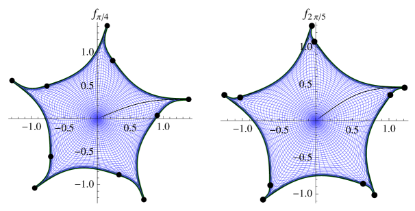
Figure 5. For $n=5$ with $\beta=\pi/4$ (left) and $\beta=2\pi/5$ (right), the nodes and cusps are indicated by a dots, and interlace with one another by argument. The argument of each node and cusp increases with $\beta$ by equation (3.8). Node and cusp locations are as described $\left|\beta\right|<\pi/2$ in Theorem 4.16.

By Corollary 4.10, the rosette harmonic mappings $f_{\beta}$ for $\left|\beta\right|<\pi/2$ have $n$-cusps, just as for the $n$-cusped hypocycloid mappings. Moreover with $n$ fixed, corresponding cusps for different mappings have cusp axes that are parallel. This can be seen in Figure 5 and in Figure 4 where cusps $\alpha_{\beta}\left(0\right)$ have axes parallel to the real axis. The parallelism of axes follows from the identical unit tangent values of the boundary extensions, which also explains the total curvature of $\pi-2\pi/n$ from one cusp to the next, described both in Proposition 4.4 and Corollary 4.10.

The last graph $f_{\pi/2}\left(U\right)$ in Figure 4 does not have cusps, but nodes with an acute interior angle, which we now examine.

Corollary 4.11.

Let $\alpha_{\pi/2}\left(t\right)=f_{\pi/2}\left(e^{it}\right),$ and let $k=1,2,...,n.$ On the first half of the interval $\left(\left(2k-2\right)\pi/n,2k\pi/n\right),\$the total curvature of $\alpha_{\pi/2}$ is $\pi/2-\pi/n,$ while $\alpha_{\pi/2}$ is constant otherwise. There is a piecewise smooth parametrization $\tilde{\alpha}_{\pi/2},$ with the same graph as $\alpha_{\pi/2}$ over $\partial U$, and just $n$ singular points at $\tilde{\alpha}_{\pi/2}\left(2k\pi/n\right)=\alpha_{\pi/2}\left(2k\pi/n\right)$ which are nodes of $\tilde{\alpha}_{\pi/2}$ with interior angle $\pi/2-\pi/n.$

Proof.

Since $\alpha_{\pi/2}^{\prime}\left(t\right)=0$ on $\left(\left(2k-1\right)\pi/n,2k\pi/n\right),$ the singularities are not isolated, and moreover these intervals are arcs of constancy for the boundary function of $f_{\pi/2}$. We define $\tilde{\alpha}_{\pi/2},$ defined piecewise on $[0,2\pi)$ by

(4.11) $$\tilde{\alpha}_{\pi/2}\left(t\right)=\alpha_{\pi/2}\left(\left(k-1\right)\pi/n+t/2\right),\text{ }t\in[\left(2k-2\right)\pi/n,2k\pi/n).$$

Then on each interval in (4.11) the curve $\tilde{\alpha}_{\pi/2}$ has the values
$\alpha_{\pi/2}\left(\left[\left(2k-2\right)\pi/n,\left(2k-1\right)\pi/n\right]\right)$. Moreover, $\tilde{\alpha}_{\pi/2}\left(2k\pi/n\right)=\alpha_{\pi/2}\left(2k\pi/n\right).$ Thus $\tilde{\alpha}_{\pi/2}$ is also continuous, with the same image as $\alpha_{\pi/2}$ on $\left[0,2\pi\right].$ We compute

$$\lim_{t\rightarrow 2k\pi/n^{-}}\arg\tilde{\alpha}_{\pi/2}^{\prime}\left(t\right) =\lim_{t\rightarrow 2k\pi/n^{-}}\arg\alpha_{\pi/2}^{\prime}\left(\left(k-1\right)\pi/n+t/2\right)$$

$$=\lim_{t^{\prime}\rightarrow\left(2k-1\right)\pi/n}2k\pi/2-\left(\frac{n}{2}-1\right)t^{\prime}=k\pi-\left(\frac{n}{2}-1\right)\left(2k-1\right)\frac{\pi}{n}.$$

and using the formula for $\arg\tilde{\alpha}_{\pi/2}^{\prime}$ on $\left(2k\pi/n,2\left(k+1\right)\pi/n\right)$ obtain

$$\lim_{t\rightarrow 2k\pi/n^{+}}\arg\tilde{\alpha}_{\pi/2}^{\prime}\left(t\right) =\lim_{t\rightarrow 2k\pi/n^{+}}\arg\alpha_{\pi/2}^{\prime}\left(k\pi/n+t/2\right)$$

$$=\lim_{t^{\prime}\rightarrow 2k\pi/n}\left(2k+2\right)\pi/2-\left(\frac{n}{2}-1\right)t^{\prime}$$

$$=\left(k+1\right)\pi-\left(\frac{n}{2}-1\right)2k\frac{\pi}{n}.$$

The difference $\arg\tilde{\alpha}_{\pi/2}^{\prime}\left(2k\pi/n\right)^{+}-\arg\tilde{\alpha}_{\pi/2}^{\prime}\left(2k\pi/n\right)^{-}$ is thus $\pi-\left(\frac{n}{2}-1\right)\pi/n=\pi/2+\pi/n,$ so we have a node with interior angle $\pi/2-\pi/n.$ ∎

Remark 4.12.

The node $\tilde{\alpha}_{\pi/2}\left(2k\pi/n\right)$ can be written $e^{i2k\pi/n}\alpha_{\pi/2}\left(t\right)$ for any
$t\in\left[\left(2k-1\right)\pi/n,2k\pi/n\right],$ where $\alpha_{\pi/2}$ is constant. We write the nodes of $\tilde{\alpha}_{\pi/2}$ as
$e^{i2k\pi/n}f_{\pi/2}\left(1\right)$ when convenient, and refer to nodes of $\tilde{\alpha}_{\pi/2}$ as the nodes of $f_{\pi/2}.$

Example 4.13.

When $\beta=\pi/2$ and with $n=5,$ then on intervals $\left(0,\pi/5\right),$ $\left(2\pi/5,3\pi/5\right),$ … the boundary arcs $e^{i\pi/4}h_{5}\left(e^{it}\right)$ and $e^{-i\pi/4}\overline{g_{5}}\left(e^{-it}\right)$ are translates of one another, and on intervals $\left(\pi/5,2\pi/5\right),$ $\left(3\pi/5,5\pi/5\right),$ …, the boundary arcs are mirrors of one another. Figure 6 (right) shows the arc of constancy $\left(\pi/5,2\pi/5\right)$ on which $\ e^{i\pi/4}h_{5}\left(e^{it}\right)$ and $e^{-i\pi/4}\overline{g_{5}}\left(e^{-it}\right)$ are mirror images, and where $f_{\pi/2}\left(e^{it}\right)$ is equal to the node $e^{i2\pi/5}f_{\pi/2}\left(1\right)$ (indicated with a larger dot in the second quadrant).

Figure 6. Images of sectors in $U$ of $e^{i\pi/4}h_{5}$ and $e^{-i\pi/4}\overline{g_{5}}$ with $\arg z\in\left(0,\pi/5\right)$ shaded (left) and $\arg z\in\left(\pi/5,2\pi/5\right)$ shaded (right), for $n=5.$ The bounding curves (thickened), are translates (left) and reflections (right). A tangent is indicated for $h_{5}\left(e^{it}\right)$ and $\overline{g_{5}\left(e^{it}\right)}$ in each case, along with a portion of $f_{\pi/2}\left(e^{it}\right)$, which is constant (right) on $\left(\pi/5,2\pi/5\right).$

We now complete our description of the symmetries within the graphs of the rosette mappings.

Corollary 4.14.

Let $\beta\in\mathbb{R}$ and $n\geq 3.$ If $\beta$ is not a multiple of $\pi/2,$ then the image set $f_{\beta}\left(U\right)$ does not have reflectional symmetry. In this case, $f_{\beta}\left(U\right)$ has symmetry group $C_{n}.$ Otherwise, $\beta$ is a multiple of $\pi/2,$ and $f_{\beta}\left(U\right)$ has symmetry group $D_{n}.$

Proof.

All rosette mappings have at least $n$ fold rotational symmetry, by Proposition 3.10 (ii). Since $f_{\beta}$ has either exactly $n$ cusps, or exactly $n$ non-removable nodes, $f_{\beta}\left(U\right)$ cannot have a higher order of symmetry. For $\left|\beta\right|\in\left(0,\pi/2\right),$ the axis of the cusp through $f_{\beta}\left(1\right)$ is parallel to the real axis, while the radial ray through $0$ and $f_{\beta}\left(1\right)$ has argument $\psi=\arg f_{\beta}\left(1\right),$ distinct for each $\beta$ in $\left(-\pi/2,\pi/2\right)$ by equation (3.8). Moreover as noted in Lemma 3.11, $\psi$ is acute, and has the same sign as $\beta.$ Thus if $\left|\beta\right|\in\left(0,\pi/2\right),$ then any reflection of $f_{\beta}\left(U\right)$ has angle of opposite signresults changing the sign of the angle between the reflected cusp axis and the reflected radial ray, resulting in a distinct reflected image set. Thus the symmetry group of $f_{\beta}\left(U\right)$ is $C_{n}$ for $\left|\beta\right|\in\left(0,\pi/2\right).$ This fact extends by formula (3.4) to any real $\beta$ that is not a multiple of $\pi/2.$ If $\beta=0$ or $\beta=\pi/2$ we already established that $f_{\beta}\left(U\right)$ has reflectional symmetry. We conclude that the sets $f_{0}\left(U\right)$ and $f_{\pi/2}\left(U\right)$ have dihedral symmetry group $D_{n}$. If $\beta=l\pi/2$ for some $l\in\mathbb{Z}$ then by formula (3.4), $f_{\beta}\left(U\right)$ is a rotation of either $f_{\pi/2}\left(U\right)$ or $f_{0}\left(U\right),$ and thus has reflectional symmetry also. ∎

Corollary 4.15.

Let $n\geq 3.$ For distinct $\beta$ and $\beta^{\prime}$ in the interval $(-\pi/2,\pi/2],$ the image sets $f_{\beta}\left(U\right)$ and $f_{\beta^{\prime}}\left(U\right)$ are not scalings or rotations of one another. Moreover with the parameter $\beta$ within the set $\left[0,\pi/2\right],$ all images of the unit disk under a rosette harmonic mapping are obtained, up to rotation and reflection.

Proof.

The proof of Corollary 4.14 shows that if $\beta\in\left(-\pi/2,\pi/2\right),$ the angle between the cusp axis through $f_{\beta}\left(1\right)$ and the radial line from $0$ to $f_{\beta}\left(1\right)$ intersect at an angle that is distinct for each choice of $\beta.$ Thus $f_{\beta}\left(U\right)$ is different from any rotation or scaling of $f_{\beta^{\prime}}\left(U\right)$ for any other $\beta^{\prime}\in\left(-\pi/2,\pi/2\right).$ Moreover $f_{\pi/2}$ is the only $f_{\beta}$ without cusps for $\beta\in(-\pi/2,\pi/2].$ To prove the second statement, let $\tilde{\beta}\in\mathbb{R}\backslash(-\pi/2,\pi/2].$ Upon reducing $\tilde{\beta}$ modulo $\pi,$ we obtain an equivalent $\beta\equiv\tilde{\beta}$ $(\operatorname{mod}$ $\pi)$ where $\beta\in(-\pi/2,\pi/2].$ By possibly repeated application of (3.3) in Proposition 3.8 (i), $f_{\tilde{\beta}}\left(z\right)$ is obtained as a pre- and post- composition of a rotation with $f_{\beta}\left(z\right).$ Thus it is sufficient to consider $\beta\in(-\pi/2,\pi/2].$ If $\beta<0,$ then by Proposition 3.8 (ii), $f_{\beta}\left(z\right)$ is a reflection in the real axis of $f_{-\beta}\left(z\right)$ where $-\beta\in\left[0,\pi/2\right].$ ∎

We turn to describing features of the graphs $f_{\beta}\left(U\right)$ for $\beta$ restricted to $(-\pi/2,\pi/2].$ We may use equation (3.4) to identify cusps and nodes for $\beta$ outside this interval, but we make the cautionary observation that while for $\beta\in\left(-\pi/2,\pi/2\right)$ $f_{\beta}\left(1\right)$ is a cusp and $f_{\beta}\left(e^{i\pi/n}\right)$ is a node, adding $\pi$ to $\beta$ results in $f_{\beta+\pi}\left(1\right)$ being a node and $f_{\beta+\pi}\left(e^{i\pi/n}\right)$ being a cusp. Quantities such as the magnitude of a cusp, the magnitude of a node, and the distribution of angle between cusps neighboring nodes however, are independent of the interval to which $\beta$ is restricted. These quantities are derived in Theorem 4.16, with the help of Lemma 3.11.

Theorem 4.16 shows that for fixed $n,$ the image $f_{0}\left(U\right)$ has maximal diameter, and $diam\left(f_{\left|\beta\right|}\left(U\right)\right)$ decreases with $\left|\beta\right|\in\left(0,\pi/2\right).\,$This is illustrated in Figure 4, where all four graphs are plotted on the same scale. We also see that for $\beta=0,$ the cusps and nodes are equally spaced with angular separation $\pi/n,$ but this becomes increasingly unbalanced as $\left|\beta\right|$ increases to $\pi/2.$ As $\beta\nearrow\pi/2^{-},$ each node approaches the subsequent cusp, as shown in Theorem 4.16 (ii).

Theorem 4.16.

Let $n\geq 3,$ $\beta\in(-\pi/2,\pi/2],$ and let $\alpha_{\beta}\left(t\right)=f_{\beta}\left(e^{it}\right)$ where $f_{\beta}$ is a rosette harmonic mapping. Recall the constant $K_{n}$ defined in Lemma 3.11.
(i)  If $\beta\in\left(-\pi/2,\pi/2\right)$ then the magnitude of the cusps decreases strictly if $\left|\beta\right|\in[0,\pi/2),$ from a maximum $K_{n}\sec\left(\frac{\pi}{2n}\right),$ and with infimum $K_{n}\left(1+\tan\left(\frac{\pi}{2n}\right)\right).$ The removable nodes have magnitudes that increase strictly if $\left|\beta\right|\in[0,\pi/2),$ from the minimum $K_{n}\left(1+\tan\left(\frac{\pi}{2n}\right)\right)$ and with supremum $K_{n}\sec\left(\frac{\pi}{2n}\right).$
(ii) If $\beta\in\left(-\pi/2,\pi/2\right)$ then the angle between a cusp neighboring node is

(4.12) $$\pi/n\pm\arctan\left(\frac{2\tan\left(\frac{\pi}{2n}\right)\sin\left(\beta\right)}{1-\tan^{2}\left(\frac{\pi}{2n}\right)}\right),$$

where we use the positive sign when the node has the more positive argument. For $\beta=0,$ the cusps and neighboring nodes are separated by equal angles of $\pi/n$. The difference in arguments of a cusp and subsequent node increases from $0$ to $2\pi/n$ with $\beta\in\left(-\pi/2,\pi/2\right)$.
(iii) For $\beta=\pi/2,$ the $n$ nodes of the rosette mapping $f_{\pi/2}$ have magnitude $K_{n}\sec\frac{\pi}{2n},$ and for the node $f_{\pi/2}\left(1\right)$ we have $\arg\left(f_{\pi/2}\left(1\right)\right)=\pi/4-\pi/\left(2n\right)$.

Proof.

We begin with (i). Due to the $\cos\beta$ term in (3.7), the cusp $\left|f_{\beta}\left(1\right)\right|$ is decreasing with $\left|\beta\right|$ and the node $\left|f_{\beta}\left(e^{i\pi/n}\right)\right|$ is increasing with $\left|\beta\right|.$ Note that

$$\sec^{2}\left(\frac{\pi}{2n}\right)\pm 2\tan\left(\frac{\pi}{2n}\right)\cos\beta=1+\tan^{2}\left(\frac{\pi}{2n}\right)\pm 2\tan\left(\frac{\pi}{2n}\right)=\left(1\pm\tan\left(\frac{\pi}{2n}\right)\right)^{2}.$$

In view of this equation, the maximum of $\left|f_{\beta}\left(1\right)\right|$ is $K_{n}\left(1+\tan\left(\frac{\pi}{2n}\right)\right)$ when $\beta=0,$ and $\left|f_{\beta}\left(1\right)\right|$ approaches $K_{n}\sec\left(\frac{\pi}{2n}\right)$ as $\beta$ approaches $\pi/2.$ Similarly, the minimum of $\left|f_{\beta}\left(e^{i\pi/n}\right)\right|$ is $K_{n}\left(1-\tan\left(\frac{\pi}{2n}\right)\right)$ when $\beta=0,$ and approaches $K_{n}\left(\sec\left(\frac{\pi}{2n}\right)\right)$ as an upper bound as $\left|\beta\right|$ approaches $\pi/2,$ proving (i). For (ii) formula (3.8) shows us $\arg f_{\beta}\left(1\right)$ and $\arg f_{\beta}\left(e^{i\pi/n}\right)$ are increasing with $\beta$ on $\left(-\pi/2,\pi/2\right).$ Clearly $\arg\left(f_{0}\left(1\right)\right)=0$ and $\arg f_{0}\left(e^{i\pi/n}\right)=\pi/n.$ Additionally we have $\arg\left(f_{\beta}\left(1\right)\right)<\pi/n<\arg f_{\beta}\left(e^{i\pi/n}\right)\,\$for $\beta\in\left(0,\pi/2\right).$ We compute the angle between this cusp and node to be $\arg f_{\beta}\left(e^{i\pi/n}\right)-\arg f_{\beta}\left(1\right)=\pi/n+\psi^{\prime}-\psi,$ and we use the arctangent formula $\arctan\psi^{\prime}-\arctan\psi=\arctan\left(\frac{\psi^{\prime}-\psi}{1+\psi^{\prime}\psi}\right)$ where $\psi^{\prime}$ and $\psi$ are as defined in equation (3.8). Thus after a short calculation we obtain formula (4.12). This difference increases from $\pi/n$ and approaches $2\pi/n$ as $\beta$ increases through the interval $[0,\pi/2)$. Now suppose that $\beta\in\left(-\pi/2,0\right).$ The reflection of the node $f_{\beta}\left(e^{i\pi/n}\right)$ in the real axis is the node $f_{-\beta}\left(e^{-i\pi/n}\right)$ of $f_{-\beta}$ and the reflection of $f_{\beta}\left(1\right)$ is the cusp $f_{-\beta}\left(1\right).$ From rotational symmetry, the angular difference between $\arg f_{-\beta}\left(1\right)$ and $\arg f_{-\beta}\left(e^{-i\pi/n}\right)$ is the same as the that of $\arg f_{-\beta}\left(e^{i2\pi/n}\right)$ and $\arg f_{-\beta}\left(e^{i\pi/n}\right).$ Again using rotational symmetry, this is $2\pi/n-\left(\psi-\psi^{\prime}\right)=\pi/n-\arctan\left(\frac{\psi^{\prime}-\psi}{1+\psi^{\prime}\psi}\right)=\pi/n-\arctan\left(\frac{2\tan\left(\frac{\pi}{2n}\right)\sin\left(-\beta\right)}{1-\tan^{2}\left(\frac{\pi}{2n}\right)}\right)=\pi/n+\arctan\left(\frac{2\tan\left(\frac{\pi}{2n}\right)\sin\left(\beta\right)}{1-\tan^{2}\left(\frac{\pi}{2n}\right)}\right)$. For (iii), with $\beta=\pi/2,$ we noted in Remark 4.12 after Corollary 4.11 that the nodes can be expressed as rotations of $f_{\pi/2}\left(1\right),$ for which we observed the stated quantities in Lemma 3.11 (i). ∎

The next example illustrates the separation of cusps and nodes as it varies with $\beta,$ as described in Theorem 4.16 (see also Figure 5). The relative proximity of a node and neighboring cusp coupled with equal total curvature of the boundary curve between any node and cusp (Corollary 4.10) gives rise to the appearance of a cresting wave at the cusp.

Example 4.17.

For $n=5,$ the arguments of the nodes and cusps of $f_{0}$ are equally spaced by $\pi/n=\pi/5.$ By Lemma 3.11, as $\beta\in[0,\pi/2)$ increases, the separation of a cusp and subsequent node grows from $\pi/5=36^{\circ}$ towards $2\pi/5=72^{\circ}.$ For $\beta=\pi/4$ this separation is $\pi/5+\arctan\sqrt{5/2-\sqrt{5}}\approx 63^{\circ},$ while for $\beta=2\pi/5$ it grows to $\pi/5+\arctan\sqrt{5/4-\sqrt{5}/4}\approx 71^{\circ}$ (see Figure 5). For a specific cusp or node $f_{\beta}\left(e^{ij_{0}\pi/n}\right),$ $\arg f_{\beta}\left(e^{ij_{0}\pi/n}\right)$ increases with $\beta$ (see proof of Theorem 4.16 (ii))$,\$which is also illustrated in Figure 5 as $\beta$ increases from $\pi/4$ to $2\pi/5.$ By Corollary 4.10, the total curvature of the boundary of $f_{\beta}$ between neighboring cusps is $\pi-2\pi/n=3\pi/5=108^{\circ}.$ The total curvature of the boundary from a cusp to a neighboring node is half of this, namely $54^{\circ}$. Figure 5 also indicates the phenomenon described in Theorem 4.16, that while both nodes and cusps “rotate counterclockwise” as $\beta\in\left(0,\pi/2\right)$ increases, the nodes do so at a greater rate..

Finally we point out that the argument of the boundary curve fails to be strictly increasing on the whole of $\partial U,$ for $\beta$ with $\left|\beta\right|\in\left(0,\pi/2\right).$

Corollary 4.18.

Let $n\geq 3$, $\beta\in\left(-\pi/2,\pi/2\right)$ and $\alpha_{\beta}$ be the boundary function of the rosette harmonic mapping $f_{\beta}.$ Then for each $k=1,2,...,n,$ $\arg\alpha_{\beta}\left(\left(2k-2\right)\pi/n\right),\$
$\arg\alpha_{\beta}\left(\left(2k-1\right)\pi/n\right),$ and $\arg\alpha_{\beta}\left(2k\pi/n\right)$ occur in increasing order, but there exists an interval on which $\arg\left(\alpha_{\beta}\left(t\right)\right)$ is decreasing.

Proof.

Theorem 4.16 (ii) shows that the angle $\gamma$ between a cusp and subsequent node is given by formula (4.12) which belongs to $\left(0,2\pi/n\right)$. Because the cusps are separated by angle $2\pi/n,$ the angle from a cusp to a subsequent node is then $2\pi/n-\gamma\in\left(0,2\pi/n\right).$ Finally with $\beta\in\left(0,\pi/2\right),$ suppose that $\arg\alpha_{\beta}\left(-\epsilon\right)\leq\psi=\arg\alpha_{\beta}\left(0\right)$ for some $-\epsilon\in\left(-\pi/n,0\right),$ but for which $\arg\alpha_{\beta}^{\prime}\left(-\epsilon\right)<\tan\psi.$ Such an $\epsilon$ exists because $\alpha_{\beta}$ satisfies (4.3) with $k=0,$ so $\arg\alpha_{\beta}^{\prime}\left(0\right)^{-}=0.$ Since $\arg\alpha_{\beta}^{\prime}\left(t\right)$ is decreasing, we have $\arg\alpha_{\beta}\left(t\right)<\psi$ for all $t\in\left(-\epsilon/2,0\right),$ and so $\alpha_{\beta}\left(t\right)$ lies in a half-plane formed by a line parallel to to $\arg z=\psi,$ but with smaller imaginary part, and this half plane does not contain $\alpha_{\beta}\left(0\right).$ This contradicts continuity of $\alpha_{\beta}\left(t\right)\rightarrow\alpha_{\beta}\left(0\right)$ as $t\nearrow 0^{-}.$ Thus there is an interval $\left(-\epsilon,0\right)$ on which $\arg\alpha_{\beta}\left(t\right)>\psi.$ On this interval, $\arg\alpha_{\beta}\left(t\right)$ decreases to $\psi,$ and so rotates negatively relative to the origin. A similar argument holds when $\beta\in\left(-\pi/2,0\right).$ ∎

5. Univalence and Fundamental Sets

Our approach to proving the univalence of $f_{\beta}$ is to use the argument principle for harmonic functions. We note that various proofs of univalence for rosette mappings $f_{\beta}$ are possible. The following theorem describes the winding number of the boundary curve $\alpha\left(t\right)=f_{\beta}\left(e^{it}\right),$ so that we can apply the argument principle.

Lemma 5.1.

For fixed $\beta\in[0,\pi/2),$ the boundary $\alpha_{\beta}\left(t\right)=f_{\beta}\left(e^{it}\right),$ $t\in\partial U$ is a simple, positively oriented closed curve. While $\alpha_{\pi/2}$ has arcs of constancy, the parametrization $\tilde{\alpha}_{\pi/2}$ of equation (4.11) is a simple, positively oriented closed curve on $\partial U.$

Proof.

Let $\beta\in\left(0,\pi/2\right).$ We give a separate argument for $\beta=0$ and for $\beta=\pi/2.$ We first show that $\alpha_{\beta}$ is one to one when restricted to $\left(0,2\pi/n\right),$ and that the boundary curve portion $\alpha_{\beta}\left(\left(0,2\pi/n\right)\right)$ lies in a sector $S.$ We then show that the portion of the graph of $\alpha_{\beta}$ restricted to the interval $\left(2k\pi/n,2\left(k+1\right)\pi/n\right)$ is contained within the set $e^{i2k\pi/n}S.$ The sets $\left\{e^{i2k\pi/n}S:k=0,1,...,n-1\right\}$ are then seen to be pairwise disjoint, so that the curve $\alpha_{\beta}$ has no self intersections on $[0,2\pi),$ and we conclude $\alpha_{\beta}$ is a simple closed curve on $\partial U.$

Define $L_{k}$ to be the axis of the cusp $\alpha_{\beta}\left(2k\pi\right),$ so with argument equal to $2k\pi/n,$ $k=0,1,..,n-1.$ Recall from Theorem (4.9) that $\alpha_{\beta}$ satisfies (4.2) (which holds except at $t=\left(2k+1\right)\pi/n$). We begin with $\alpha_{\beta}$ on the interval $\left(0,2\pi/n\right).$ Let $p$ be the intersection of $L_{0}$ (parallel to the real axis) and $L_{1}.$ These non-collinear lines form the boundary of four unbounded open connected sectors, and we define $S$ to be the sector with vertex $p$  for which the (distinct) cusps $\alpha_{\beta}\left(0\right)\in L_{0}$ and $\alpha_{\beta}\left(2\pi/n\right)\in L_{1}$ belong to $\partial S.$ By equation (4.2), $\arg\alpha_{\beta}^{\prime}\left(t\right)$ is decreasing and $\arg\alpha_{\beta}^{\prime}\left(0\right)^{+}=\pi.$ Thus the curve $\alpha_{\beta}$ lies “above” $L_{0}$. If $\alpha_{\beta}$ were to cross $L_{1}$ at some $t_{1}\in\left(0,2\pi/n\right),$ then $\arg\alpha_{\beta}^{\prime}\left(t_{1}^{\prime}\right)<2\pi/n$ for some $t_{1}^{\prime}\in\left(t_{1},2\pi/n\right)$ in order for $\arg\alpha_{\beta}^{\prime}\left(2\pi/n\right)^{-}=2\pi/n$ in equation (4.3) to hold. However $\arg\alpha_{\beta}^{\prime}\left(\left(0,2\pi/n\right)\right)\subset\left(2\pi/n,\pi\right)$ so no such intersection can occur, and we conclude that $\alpha_{\beta}$ restricted to $\left(0,2\pi/n\right)$ lies within the region $S.$ Moreover, because $\arg\alpha_{\beta}^{\prime}\left(t\right)$ decreases strictly, with total change $\pi-2\pi/n<\pi,$ $\alpha_{\beta}$ must be one to one on $\left(0,2\pi/n\right).$ Now let $k=1,2,..,n,$ and consider the curve $\alpha_{\beta}$ restricted to $\left(2k\pi/n,2\left(k+1\right)\pi/n\right).$ By rotational symmetry of $f_{\beta}$, $\alpha_{\beta}\left(t+2k\pi/n\right)=e^{i2k\pi/n}\alpha_{\beta}\left(t\right)$, $\alpha_{\beta}$ is also one to one on $\left(2k\pi/n,2\left(k+1\right)\pi/n\right)$, and the graph $\alpha_{\beta}\left(\left(2k\pi/n,2\left(k+1\right)\pi/n\right)\right)\subseteq e^{i2k\pi/n}S.$ We complete the proof for $\beta\in\left(0,\pi/2\right)$ by showing that the sets $\left\{e^{i2k\pi/n}S:k=0,1,...,n-1\right\}$ are pairwise disjoint. Because of rotational symmetry, the line $e^{i2k\pi/n}L_{0}$ passes through $e^{i2k\pi/n}\alpha_{\beta}\left(0\right)=\alpha_{\beta}\left(2k\pi/n\right),$ a cusp, and $e^{i2k\pi/n}L_{0}$ has argument $2k\pi/n,$ so $e^{i2k\pi/n}L_{0}=L_{k}.$ Similarly $e^{i2k\pi/n}L_{1}=L_{k+1}.$ Thus $e^{i2k\pi/n}S$ is a sector with sides $L_{k}$ and $L_{k+1},$ and vertex at their point of intersection $e^{i2k\pi/n}p.$ The points $\left\{e^{i2k\pi/n}p:k=0,..,n-1\right\}$ form the vertices of a regular $n$-gon, that we denote by $P.$ Then $P$ is centered on the origin, and we have $\operatorname{Im}p>0,$ since the cusp $\alpha_{\beta}\left(0\right)$ has argument $\psi=\arg\alpha_{\beta}\left(0\right)\in\left(0,\pi/4\right)$ by Lemma 3.11 (ii). Note also that $L_{n}=L_{0},$ and $L_{n-1}=e^{-i2\pi/n}L_{0}.$ Thus $L_{0}$ and $L_{n-1}$ intersect at $e^{-i2\pi/n}p,$ with $\operatorname{Im}\left(e^{-i2\pi/n}p\right)=\operatorname{Im}\left(p\right).$ Therefore $p$ is in the second quadrant, and $e^{-i2\pi/n}p$ is in the first quadrant. We conclude that one bounding side of the sector $S$ is $\left\{z\in L_{0}:\arg z\leq\arg p\right\}$. By rotational symmetry, the second side of $S$ is $\left\{z\in L_{1}:\arg z\leq 2\pi/n+\arg p\right\}$. Thus the rays $\left\{z\in L_{k}:\arg z\leq 2k\pi/n+\arg p\right\}$ that extend the sides of $P,$ each originating at $e^{i2k\pi/n}p$ and extending in the direction of decreasing argument, form the boundaries of the sectors $e^{i2k\pi/n}S,$ where $k=0,1,...,n-1$ (see Figure 7 (left) where $S$ is shaded).

Figure 7. The sector $S$ and regular $n$-gon $P$ (left). The set $S^{\prime}$ lies on the non-zero side of the line $L_{0},$ and is bounded by $L_{0}^{\prime}$ and $L_{1}^{\prime}$ (right).

Various approaches are possible to demonstrate that the sectors $e^{i2k\pi/n}S$ are disjoint. For instance, note that $\arg p=\pi/2+\pi/n,$ and consider the related sector

$$S^{\prime}=\left\{z\in\text{ext}\left(P\right):\arg z\in[\pi/2-\pi/n,\pi/2+\pi/n)\right\}.$$

The sets $e^{i2k\pi/n}S^{\prime}$ are clearly disjoint for $k=0,1,...,n-1,$ since the arguments of points in the sets $e^{i2k\pi/n}S^{\prime}$ for distinct $k\in\left\{0,1,...,n-1\right\}$ are in disjoint intervals (see the right of Figure 7, where $S^{\prime}$ is region that is shaded). Let $L_{k}^{\prime}$ be the line through the origin and with argument $\pi/2+\left(2k-1\right)\pi/n,$ and let $E$ be the set $E=\left\{z\in ext\left(P\right):\arg z<\pi/2-\pi/n,\text{ }\operatorname{Im}z\geq\operatorname{Im}p\right\},$ bounded by $L_{0}$ and $L_{0}^{\prime}$ and $P.$ We obtain $S$ from $S^{\prime}$ by including the set $E,$ and excluding the set $e^{i2k\pi/n}E$ (darker shaded region in the right of Figure 7) from $S^{\prime}.$ Then $S=S^{\prime}\cup E\backslash e^{i2\pi/n}E,$ and by rotational symmetry,

$$e^{i2k\pi/n}S=e^{i2k\pi/n}S^{\prime}\cup e^{i2k\pi/n}E\backslash e^{i2\left(k+1\right)\pi/n}E.$$

Thus to obtain $e^{i2k\pi/n}S$ we have simply removed a sector with vertex $e^{i2\left(k-1\right)\pi/n},$ namely $e^{i2k\pi/n}E,$ from the set $e^{i2k\pi/n}S^{\prime}$ and included its rotation $e^{i2\left(k+1\right)\pi/n}E$ to obtain $e^{i2\left(k+1\right)\pi/n}S^{\prime}.$ Because the sets $e^{i2k\pi/n}S^{\prime}$ are disjoint, so are the sets $\left\{e^{i2k\pi/n}S:k=0,1,..,n-1\right\}.$

If $\beta=0$ then $p=0$ and the argument above does not apply, but a simple proof follows if we adapt the proof for $\beta\in\left(0,\pi/2\right)$ and define the sector $S$ to be $S=\left\{z\in\mathbb{C}:\arg z\in\left(0,2\pi/n\right)\right\},$ in which case the sectors $\left\{e^{2k\pi i/n}S:k=0,1,...,n-1\right\}$ are clearly disjoint.

If $\beta=\pi/2,$ then we adapt the proof so that $L_{k}$ is the line passing through node $\alpha_{\pi/2}\left(2k\pi/n\right)$ with argument $\alpha_{\pi/2}^{\prime}\left(2k\pi/n\right)^{+}$. The sectors then are bounded by the lines $L_{k},$ and the same same argument applies to show $\tilde{\alpha}_{\pi/2}$ is one to one on $S$ (note that $\arg\tilde{\alpha}_{\pi/2}\left(\left(0,2\pi/n\right)\right)\subset\left(\pi/2+\pi/\left(2n\right),\pi\right)$ rather than $\arg\alpha_{\beta}^{\prime}\left(\left(0,2\pi/n\right)\right)\subset\left(2\pi/n,\pi\right)$). ∎

Theorem 5.2.

For any $n\geq 3$ in $\mathbb{N},$ the harmonic functions $f_{\beta}\left(z\right)$, $\beta\in\mathbb{R}$ defined in Definition 3.5 are univalent, and so they are harmonic mappings.

Proof.

We apply the argument principle for harmonic functions of [DHL96] to obtain univalence of $f_{\beta}.$ We proved in Lemma 5.1 that for $\beta\in[0,\pi/2),$ the boundary curve $\alpha_{\beta}\left(t\right)=f_{\beta}\left(e^{it}\right)$ on $\partial U$ is a simple closed curve about the origin. Although $\alpha_{\pi/2}$ has arcs of constancy, the winding number about each point enclosed by the curve $\alpha_{\beta}$ is still $1,$ so the argument principle applies for $\beta=\pi/2$. Choose an arbitrary point $w_{0}$ enclosed by the curve $\alpha_{\beta}.$ Then define $f=f_{\beta}-w_{0},$ a harmonic function continuous in $\bar{U}$, which does not have a zero on $\partial U$. Moreover, since $\left|\omega_{f}\right|=\left|\omega\right|<1$ in $U$, $f$ does not have any singular zeros in $U$. We see that $f\left(e^{it}\right)=\alpha_{\beta}\left(t\right)-w_{0}$ has index 1 about the origin for $t\in\partial U$, so it follows from the argument principle that $f$ has exactly one zero in $U$. Thus $f_{\beta}\left(z_{0}\right)=w_{0}$ for a unique $z_{0}\in U.$ Since the choice of $z_{0}\in U$ was arbitrary, we see that $f_{\beta}$ is onto the region enclosed by $\alpha_{\beta}.$ If $w_{1}$ is in the exterior of the region enclosed by the curve $\alpha_{\beta},$ then consider the function $\tilde{f}=$ $f_{\beta}-w_{1}.$ The harmonic function $\tilde{f}$ satisfies the same hypotheses as did $f,$ but the winding number of $\tilde{f}\left(e^{it}\right)$ about the origin is zero. Thus there is no $z_{1}\in U$ for which $f_{\beta}\left(z_{1}\right)=w_{1}.$ Therefore $f_{\beta}\left(U\right)$ is contained in the interior of the region bounded by $\alpha_{\beta}.$ If $\beta\in(-\pi/2,0),$ then $f_{\beta}$ is univalent since it is a reflection of $f_{-\beta}$ where $-\beta>0.$ Finally if $\beta\not\in(-\pi/2,\pi/2]$ then $f_{\beta}\left(z\right)$ is a rotation of $f_{\beta}\left(e^{-il\pi/n}z\right)$ for some $l\in\mathbb{Z}$ by Corollary 3.9, so is also univalent. ∎

Remark 5.3.

On sectors $S$ of the closed unit disk for which $g_{n}\left(S\right)$ is convex, we can show that $g_{n}$ is relatively more contractive than $h_{n},$ in that for any two points $z_{0}$ and $z_{1}$ in the sector,

$$\left|h_{n}\left(z_{0}\right)-h_{n}\left(z_{1}\right)\right|\geq\left|g_{n}\left(z_{0}\right)-g_{n}\left(z_{1}\right)\right|$$

Moreover the inequality is strict when at least one point is not on $\partial U.$ This fact can be used to show that $f_{\beta}$ is one to one in the sectors $S$ of $\bar{U}$ with argument in the range $[0,\pi/n)$, or with argument in the range $[\pi/n,2\pi/n).$ This leads to a direct proof of univalence that does not rely on the argument principle.

We now define a fundamental set, rotations of which make up the graph of the rosette harmonic mapping $f_{\beta}$. This set has an interesting decomposition into two curvilinear triangles when $\beta=0,$ or into a curvilinear triangle and curvilinear bigon for $\left|\beta\right|\in(0,\pi/2]$. Moreover, the triangle is nowhere convex for $\left|\beta\right|\in(0,\pi/2],$ and when $\beta=\pi/2$ the bigon has reflectional symmetry.

Definition 5.4.

For an interval $I$ with $\left|I\right|<2\pi,$ define the sector $S_{I}$ of the closed unit disk $\bar{U}$ to be $S_{I}=\left\{z\in\bar{U}:\arg z\in I,\text{ }0\leq r\leq 1\right\}$. For $n\in\mathbb{N},$ $n\geq 3,$ $\beta\in(-\pi/2,\pi/2],$ let $f_{\beta}$ be the rosette mapping defined in Definition 3.5, and define the fundamental set of the rosette mapping $f_{\beta}$ to be

$$\mathcal{A}_{\beta,n}=f_{\beta}\left(S_{[0,2\pi/n)}\right)=\left\{f_{\beta}\left(z\right):0\leq\left|z\right|\leq 1,\text{ }0\leq\arg z<2\pi/n\right\}.$$

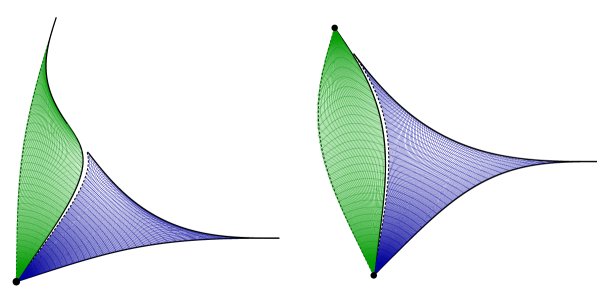
Figure 8. Fundamental sets $\mathcal{A}_{\pi/5,5}$ (left) and $\mathcal{A}_{\pi/2,5}$ (right)

The univalence of $f_{\beta}$ implies that the set $f_{\beta}\left(S_{[a,b)}\right)$ is bounded by the image of $f_{\beta}\left(\partial S_{[a,b)}\right),$ for $\left|b-a\right|<2\pi.$ Thus the fundamental set $\mathcal{A}_{\beta,n}$ is bounded by $f_{\beta}\left(\partial S_{[0,2\pi/n)}\right).$ Definition 5.4 and the following proposition apply only to $\beta\in(-\pi/2,\pi/2],$ but we will use the fundamental sets $\mathcal{A}_{\beta,n}$ with $\beta$ from this restricted range to express the graph of the rosette mapping $f_{\tilde{\beta}}\left(\bar{U}\right),$ for any $\tilde{\beta}\in\mathbb{R}.$

For $\beta\in(-\pi/2,\pi/2]$ we note a further interesting decomposition in Proposition 5.5 of the set $\mathcal{A}_{\beta,n}$ for $\beta\neq 0$ into a curvilinear triangle with sides that are nowhere convex, and a curvilinear bigon, the latter having reflectional symmetry when $\beta=\pi/2$ (see Figure 8).

Proposition 5.5.

Let $n\in\mathbb{N},$ $n\geq 3$ and $\beta\in(-\pi/2,\pi/2].$ Let $\mathcal{A}_{\beta,n}$ be the fundamental set defined in 5.4 for the rosette mapping $f_{\beta}$ of Definition 3.1. The set $\mathcal{A}_{\beta,n}$ is a curvilinear triangle subtending an angle of $2\pi/n$ at the origin. Moreover, $\mathcal{A}_{\beta,n}$ is the disjoint union

$$\mathcal{A}_{\beta,n}=f_{\beta}\left(S_{[0,\pi/n)}\right)\cup f_{\beta}\left(S_{[\pi/n,2\pi/n)}\right).$$

(i) For $\beta\in\left(0,\pi/2\right)$, the set $f_{\beta}\left(\partial S_{[0,\pi/n)}\right)$ is a curvilinear triangle with sides that are nowhere convex. The set $f_{\beta}\left(\partial S_{[\pi/n,2\pi/n)}\right)$ is a curvilinear bigon, where one side is strictly convex, and the other side has a single inflection point. The angle subtended at the origin, both by the bigon and the triangle, is $\pi/n.$ The remaining angles in the bigon and triangle are $0.$
(ii) If $\beta=\pi/2$ then the statements in (i) hold, except the angle subtended by the bigon at the node of $f_{\pi/2}$ is $\pi/2-\pi/n.$ Additionally, the bigon $f_{\pi/2}\left(\partial S_{[\pi/n,2\pi/n)}\right)$ is symmetric about the line through the vertices of the bigon.
(iii) When $\beta\in\left(-\pi/2,0\right)$, the conclusions of (i) except $f_{\beta}\left(\partial S_{[\pi/n,2\pi/n)}\right)$ is the curvilinear triangle and $f_{\beta}\left(\partial S_{[0,\pi/n)}\right)$ is the curvilinear bigon.
(iv) When $\beta=0,$ the sides of $f_{\beta}\left(\partial S_{[0,\pi/n)}\right)$ and $f_{\beta}\left(\partial S_{[\pi/n,2\pi/n)}\right)$ incident with the origin are line segments, and the curvilinear triangles $f_{\beta}\left(\partial S_{[0,\pi/n)}\right)$ and $f_{\beta}\left(\partial S_{[\pi/n,2\pi/n)}\right)$ are reflections of one another in the line containing their common side.

Proof.

We let $\alpha_{\beta}\left(t\right)=f_{\beta}\left(e^{it}\right)$ on $\partial U.$ The proofs that follow combine facts about the image of $f_{\beta}$ along radial lines of $U$ in Lemma 3.11, and limits of $\arg\alpha_{\beta}^{\prime}$ at cusps and nodes. The image $\mathcal{A}_{\beta,n}=f_{\beta}\left(S_{[0,2\pi/n)}\right)$ is bounded by $f_{\beta}\left(\partial S_{[0,2\pi/n)}\right).$ Since $f_{\beta}\left(1\right)$ and $f_{\beta}\left(e^{i2\pi/n}\right)$ are distinct, $f_{\beta}\left(\partial S_{[0,2\pi/n)}\right)$ is a curvilinear triangle (even when $\beta=\pi/2$). At the origin, Lemma 3.11 (ii) states that $f_{\beta}\left(r\right)$ and $f_{\beta}\left(re^{i\pi/n}\right)$ have tangents with arguments $\beta/2$ and $\beta/2+\pi/n.$ The side $f_{\beta}\left(re^{i2\pi/n}\right)$ is a rotation by $2\pi/n$ of $f_{\beta}\left(r\right),$ and so the argument of its tangent at $0$ is $\beta/2+2\pi/n.$ Thus the angle subtended by the vertex of $\mathcal{A}_{\beta,n}$ at the origin is $2\pi/n$. We now prove (i). Our observations about $\frac{\partial}{\partial r}\arg f_{\beta}\left(r\right),$ $\frac{\partial}{\partial r}\arg f_{\beta}\left(re^{i\pi/n}\right),$ and $\frac{\partial}{\partial r}\arg f_{\beta}\left(re^{i2\pi/n}\right)$ at the origin show that the angle subtended by $f_{\beta}\left(\partial S_{[0,\pi/n)}\right)$ and by $f_{\beta}\left(\partial S_{[\pi/n,2\pi/n)}\right)$ at the origin is $\pi/n.$ At the boundary, we have by equation (4.10) with $k=1$ in Corollary 4.10 that $\arg\alpha_{\beta}^{\prime}\left(t\right)\rightarrow\pi/2+\pi/n$ as $t\rightarrow\pi/n^{+}.$ This matches $\frac{\partial}{\partial r}\arg f_{\beta}\left(re^{i\pi/n}\right)$ at $f_{\beta}\left(e^{i\pi/n}\right)=\alpha_{\beta}\left(\pi/n\right)$, by Lemma 3.11 (ii). Thus $f_{\beta}\left(re^{i\pi/n}\right)$ and $\alpha_{\beta}\left(t\right)$ join to form a single smooth curve, together forming one side of $f_{\beta}\left(\partial S_{[0,2\pi/n)}\right),$ whence the bigon. From Lemma 3.11 (ii), $\frac{\partial}{\partial r}\arg f_{\beta}\left(re^{i\pi/n}\right)$ is strictly increasing, yet $\arg\alpha_{\beta}^{\prime}\left(e^{it}\right)$ is strictly decreasing by (4.2). Thus $f_{\beta}\left(e^{i\pi/n}\right)$ is an inflection point where curvature changes sign on the bigon. We also have $\frac{\partial}{\partial r}\arg f_{\beta}\left(r\right)$ is strictly decreasing, while $\frac{\partial}{\partial r}\arg f_{\beta}\left(re^{i\pi/n}\right)$ is strictly increasing. Thus the sides of the triangle $f_{\beta}\left(\partial S_{[0,\pi/n)}\right)$ are nowhere convex. Returning to the bigon, we now see that its second side $f_{\beta}\left(re^{i2\pi/n}\right)$ is strictly convex, since $f_{\beta}\left(re^{i2\pi/n}\right)$ is a rotation about the origin of $f_{\beta}\left(r\right)$. We complete the proof of (i) by observing that when $\beta\in[0,\pi/2),$ the vertices $f_{\beta}\left(e^{i2\pi/n}\right)$ and $f_{\beta}\left(1\right)$ are cusps of $\alpha_{\beta},$ and the angle subtended at $f_{\beta}\left(e^{i2\pi/n}\right)$ and $f_{\beta}\left(1\right)$ is $0.$

Now we turn to (ii), with $\beta=\pi/2.$ We observed reflectional symmetry in Theorem 3.10 (iii) of $f_{\pi/2}\left(re^{-i\pi/n}\right)$ and $f_{\pi/2}\left(r\right)$ about the axis through $0$ and the node $f_{\pi/2}\left(1\right).$ Rotating by $2\pi/n$, the ray through $0$ and the node $f_{\pi/2}\left(e^{i2\pi/n}\right)$ is also an axis of reflectional symmetry, in which the sides $f\left(re^{i\pi/n}\right)$ and $f\left(re^{i2\pi/n}\right)$ of the bigon are reflected. To see the subtended angle at the boundary $\alpha_{\pi/2}$, we use Lemma 3.11 (ii) as above to see the tangent of $f_{\pi/2}\left(re^{i\pi/n}\right)$ approaches $\pi/2+\pi/n$ as $r\rightarrow 1^{-}.$ By the formula in the proof of Corollary 4.11 with $k=1$, $\arg\tilde{\alpha}_{\pi/2}^{\prime}\left(t\right)$ also approaches $\pi/2+\pi/n$ as $t\rightarrow 2\pi/n^{-}.$ We conclude that the side $f_{\pi/2}\left(re^{i\pi/n}\right)$ of the bigon becomes tangent to the boundary $\tilde{\alpha}_{\pi/2}$ at the node $f_{\pi/2}\left(e^{i\pi/n}\right)=f_{\pi/2}\left(e^{i2\pi/n}\right)$ as $t\rightarrow 2\pi/n^{-}.$ By reflectional symmetry, the second side of the bigon $f_{\pi/2}\left(re^{i2\pi/n}\right)$ becomes tangent to the boundary $\tilde{\alpha}_{\pi/2}$ at as $t\rightarrow 2\pi/n^{+}.$ Thus the angle subtended in the bigon at $f_{\pi/2}\left(e^{i2\pi/n}\right)$ is the same as the interior angle of the nodes of $\tilde{\alpha}_{\pi/2},$ namely $\pi/2-\pi/n$ by Corollary 4.11.

The statements in (iii) follow readily using reflectional symmetry. For (iv) we already noted in Lemma 3.11 (iii) that the images of $f_{0}\left(r\right),$ $f_{0}\left(re^{i\pi/n}\right)$ and $f_{0}\left(re^{i2\pi/n}\right)$ are linear. Reflectional symmetry was established in Corollary 4.14. ∎

We finish by decomposing the graph of an arbitrary rosette mapping  into a disjoint union of $n$ rotations of a fundamental set of Definition 5.4.

Corollary 5.6.

Let $n\geq 3$ and $\tilde{\beta}\in\mathbb{R}.$ The set $f_{\tilde{\beta}}\left(\bar{U}\right)$ can be written as a disjoint union of rotations of $\mathcal{A}_{\beta,n}.$ Specifically if $\tilde{\beta}=\beta+l\pi$ for $\beta\in(-\pi/2,\pi/2]$ then

$$f_{\tilde{\beta}}\left(\bar{U}\right)=i^{l}{\displaystyle\bigcup_{k=1}^{n}}e^{i\left(2k+l\right)\pi/n}\mathcal{A}_{\beta,n}.$$

Proof.

By Corollary 3.9 we have $f_{\tilde{\beta}}\left(z\right)=e^{il\left(\pi/n+\pi/2\right)}f_{\beta}\left(e^{-il\pi/n}z\right).$ Thus

$$f_{\tilde{\beta}}\left(\bar{U}\right)=f_{\tilde{\beta}}\left(e^{il}\bar{U}\right)=e^{il\left(\pi/n+\pi/2\right)}f_{\beta}\left(\bar{U}\right)=i^{l}e^{il\pi/n}{\displaystyle\bigcup_{k=1}^{n}}e^{i2k\pi/n}\mathcal{A}_{\beta,n}.$$

∎

References

- [AM21] Sohair Abdullah and Jane McDougall, Rosette minimal surfaces, 2021, In Preparation.
- [BDM+12] Michael A. Brilleslyper, Michael J. Dorff, Jane M. McDougall, James S. Rolf, Lisbeth E. Schaubroeck, Richard L. Stankewitz, and Kenneth Stephenson, Explorations in complex analysis, Classroom Resource Materials Series, Mathematical Association of America, Washington, DC, 2012. MR 2963949
- [BLW15] Daoud Bshouty, Erik Lundberg, and Allen Weitsman, A solution to Sheil-Small’s harmonic mapping problem for polygons, Proc. Amer. Math. Soc. 143 (2015), no. 12, 5219–5225. MR 3411139
- [CSS84] J. Clunie and T. Sheil-Small, Harmonic univalent functions, Ann. Acad. Sci. Fenn. Ser. A I Math. 9 (1984), 3–25. MR 85i:30014
- [DHL96] Peter Duren, Walter Hengartner, and Richard S. Laugesen, The argument principle for harmonic functions, Amer. Math. Monthly 103 (1996), no. 5, 411–415. MR 97f:30002
- [DMS05] Peter Duren, Jane McDougall, and Lisbeth Schaubroeck, Harmonic mappings onto stars, J. Math. Anal. Appl. 307 (2005), no. 1, 312–320. MR 2138992 (2006c:31002)
- [DT00] Peter Duren and William R. Thygerson, Harmonic mappings related to Scherk’s saddle-tower minimal surfaces, Rocky Mountain J. Math. 30 (2000), no. 2, 555–564. MR MR1786997 (2001i:58019)
- [Dur04] Peter Duren, Harmonic mappings in the plane, Cambridge Tracts in Mathematics, vol. 156, Cambridge University Press, Cambridge, 2004. MR 2 048 384
- [HS86] W. Hengartner and G. Schober, On the boundary behavior of orientation-preserving harmonic mappings, Complex Variables Theory Appl. 5 (1986), no. 2-4, 197–208. MR 846488
- [JS66] Howard Jenkins and James Serrin, Variational problems of minimal surface type. II. Boundary value problems for the minimal surface equation, Arch. Rational Mech. Anal. 21 (1966), 321–342. MR MR0190811 (32 #8221)
- [Lew36] H. Lewy, On the non-vanishing of the jacobian in certain one-to-one mappings, Bull. Amer. Math. Soc. 42 (1936), no. 1, 689–692.
- [McD12] Jane McDougall, Harmonic mappings with quadrilateral image, Complex analysis and potential theory, CRM Proc. Lecture Notes, vol. 55, Amer. Math. Soc., Providence, RI, 2012, pp. 99–115. MR 2986895
- [MS61] E. P. Merkes and W. T. Scott, Starlike hypergeometric functions, Proc. Amer. Math. Soc. 12 (1961), 885–888. MR 0143950
- [MS08] Jane McDougall and Lisbeth Schaubroeck, Minimal surfaces over stars, J. Math. Anal. Appl. 340 (2008), no. 1, 721–738. MR 2376192
- [Rai71] Earl D. Rainville, Special functions, first ed., Chelsea Publishing Co., Bronx, N.Y., 1971. MR 0393590
- [Sch72] H. A. Schwarz, Gesammelte mathematische Abhandlungen. Band I, II, Chelsea Publishing Co., Bronx, N.Y., 1972, Nachdruck in einem Band der Auflage von 1890. MR MR0392470 (52 #13287)
- [SS89] T. Sheil-Small, On the Fourier series of a step function, Michigan Math. J. 36 (1989), no. 3, 459–475. MR 91b:30002