An Accurate Reconstruction of CMB E Mode Signal over Large Angular Scales using Prior Information of CMB Covariance Matrix in ILC Algorithm

Abstract

In the recent years, the internal-linear-combination (ILC) method was investigated extensively in the context of reconstruction of Cosmic Microwave Background (CMB) temperature anisotropy signal using observations obtained by WMAP and Planck satellite missions. In this article, we, for the first time, apply the ILC method to reconstruct the large scale CMB E mode polarization signal, which serves as the unique probe of ionization history of the Universe, using simulated observations of $15$ frequency CMB polarization maps of future generation Cosmic Origin Explorer (COrE) satellite mission. We find that usual ILC cleaned E mode map is highly erroneous due to presence of a chance-correlation between CMB and astrophysical foreground components in the empirical covariance matrix which is used to estimate the weight factors. The cleaned angular power spectrum for E mode is strongly biased and erroneous due to these chance correlation factors. In order to address the issues of bias and errors we extend and improve the usual ILC method for CMB E mode reconstruction by incorporating prior information of theoretical E mode angular power spectrum while estimating the weights for linear combination of input maps (Sudevan & Saha 2018b). Using the E mode covariance matrix effectively suppresses the CMB-foreground chance correlation power leading to an accurate reconstruction of cleaned CMB E mode map and its angular power spectrum. We provide a comparative study of the performance of the usual ILC and the new method over large angular scales of the sky and show that the later produces significantly statistically improved results than the former. The new E mode CMB angular power spectrum contains neither any significant negative bias at the low multipoles nor any positive foreground bias at relatively higher mutlipoles. The error estimates of the cleaned spectrum agree very well with the cosmic variance induced error.

¹Department of Physics, Indian Institute of Science Education and Research, Bhopal-462066, India

Keywords: CMB anomalies, CMB Phase analysis, CMB non-gaussianity

1 Introduction

Weakly polarized component of the Cosmic Microwave Background (CMB) anisotropy  (Rees, 1968; Basko & Polnarev, 1980) serves as an important probe (Spergel & Zaldarriaga, 1997; Zaldarriaga & Seljak, 1998; Knox & Song, 2002) to understand different evolutionary epochs in the expanding Universe. The E mode component of the polarized CMB signal over large angular scales of the sky is sensitive to interactions of CMB photons with the free electrons in space and therefore is a potential observable to tightly constrain the ionization history of the Universe (Page et al., 2007; Burigana et al., 2008; Planck Collaboration et al., 2016b; Watts et al., 2019). On the very large angular scales the CMB E mode signal is dominated by the secondary anisotropies generated during the scattering of CMB photons with the high energy electrons produced after galaxies were formed. The peak height and location of EE mode CMB angular power spectrum on the large angular scales are determined by the amount of the free electrons present in the inter galactic medium and epoch of reionization respectively. On the scales $\ell\lesssim 15$ the EE mode spectrum can be used to constrain the physics at the last scattering surface as well. In the era of precision measurement of cosmological parameters CMB E mode signal provide accurate measures of amplitude of scalar field fluctuations and the optical depth of reionization epoch by breaking degeneracies between the two.

In order to extract the complete set of cosmological information available from CMB E mode signal on large angular scales one needs to perform an accurate reconstruction of the CMB E mode map on these scales. This, however, is a challenging task since the weak E mode CMB signal remains hidden inside the weakly understood, strong polarized foreground signals due to synchrotron and thermal dust emissions that originate from the Milky Way. An important method for removing foregrounds from observed CMB maps is the so-called internal-linear-combination (ILC) technique (Bennett et al., 1992; Tegmark & Efstathiou, 1996; Bennett et al., 2003; Tegmark & Efstathiou, 1996; Gold et al., 2011). The method was applied on WMAP observations to estimate the CMB temperature anisotropy angular power spectrum by Saha et al. (2006) and subsequently extensively studied (Saha et al., 2008) and applied on WMAP and Planck observations  (Sudevan et al., 2017) following a new improved version, the iterative ILC algorithm in harmonic space which removes a foreground leakage signal in the final cleaned map. Sudevan & Saha (2018a) proposed and implemented a new ILC algorithm on large angular scales of the sky on CMB temperature anisotropy observations of WMAP and Planck using prior information of CMB covariance matrix. This method, by effectively suppressing dominant CMB-foregrounds chance correlations at large angular scales, reconstructed a cleaned map and its angular power spectrum accurately without any bias. Sudevan & Saha (2018b) developed a new model independent method, the Gibbs ILC method, to estimate the joint CMB posterior density and CMB theoretical angular power spectrum given the observed foreground contaminated CMB anisotropy data at large angular scales of the sky. They provided the best fit estimates of both, CMB temperature map and theoretical angular power spectrum along with their confidence interval regions which can directly be integrated to cosmological parameter estimation process. In another article Sudevan & Saha (2020) the authors have investigated in detail the impact of random residual error in calibration coefficients corresponding to observed CMB maps on the Gibbs ILC estimates at large angular scales.

The ILC method is very appealing since the weights that are used for linear combinations of the input foreground contaminated maps are obtained by a simple analytical expression. The advantage of the ILC method is that in order to reconstruct the CMB map one does not require to model foreground components, neither in terms of their frequency spectrum nor in terms of any templates that trace the morphological pattern of a foreground components across the sky. This greatly reduces the complexity which is otherwise involved in a complete component reconstruction technique, in which all foregrounds and CMB component are required to be simultaneously and explicitly modelled in order to even reconstruct just the single CMB component. Since the foreground modelling is not necessary in an ILC method the cleaned CMB map and its angular power spectrum are, therefore, not affected by any error induced by the uncertainties in the assumed foreground model. Although a significant amount of research have already been performed to reconstruct CMB temperature anisotropy signal using the foreground model independent method its performance on CMB polarization signal reconstruction remains yet to be evaluated. During the CMB temperature analysis at large angular scales Sudevan & Saha (2018a) reported a large error while reconstructing the CMB signal using usual ILC method. A detailed investigation revealed that it is due to the presence of CMB-foreground chance correlation at large angular scales and the usual ILC weights were not able to minimize this chance correlation power during linear combination. The authors then proposed a new method, the global ILC method (Sudevan & Saha, 2018a) , as a remedy since incorporating the theoretical CMB covariance matrix in the ILC algorithm effectively suppressed these chance correlations and aided in obtaining an accurate CMB map at large angular scales. A similar investigation needs to be carried out in the context of foreground removal in the CMB polarization analysis. Since CMB polarization signal is much weaker as compared to the CMB temperature, it is yet unclear what is the the role of CMB-foreground chance correlation while reconstructing a CMB polarization signal at large angular scales and one should, therefore, study in detail. In this article, we seek to obtain an answer to the question - what is the effect of CMB-foregrounds chance correlations at large angular scales on the cleaned CMB E mode map estimated using usual ILC method and how well the global ILC method reconstructs weak CMB E mode signal over large angular scales of the sky using prior information of CMB covariance matrix.

A study regarding the performance of the ILC method on CMB E mode reconstruction is necessary also due to a different reason. A new horizon in cosmology is expected to be seen with the observations from future generation satellite missions which can measure CMB polarization signal with sufficiently large signal to noise ratio to measure the weak CMB polarization signal over a wide range of angular scales. Future generation CMB polarization observations LiteBIRD (Matsumura et al., 2014; Sugai et al., 2020) , Cosmic Origin Explorer (COrE) (Delabrouille et al., 2018), Probe of Inflation and Cosmic Origin (PICO) (Hanany et al., 2019) have already been proposed. With these sensitive CMB polarization missions in the making it is again an important question to ask how accurate does the CMB reconstruction techniques perform on the simulated observations of these experiments . In this article, we apply the usual ILC and global ILC method on the E mode signals of simulated polarization observations of COrE and study the performance of each methods.

For CMB component reconstructions several methods have been proposed in the literature. Eriksen et al. (2006) proposed a parametric method for CMB and other foreground component separation. CMB component and its angular power spectrum along with foreground components are reconstructed by Eriksen et al. (2004, 2008b, 2008a); Planck Collaboration et al. (2018a, 2016a); Remazeilles et al. (2018a, b) by employing a Gibbs sampling technique. Saha (2011) estimates a foreground cleaned CMB temperature anisotropy map using WMAP observations by minimizing a measure of non Gaussianity of the foreground contaminated maps. A generalized ILC algorithm for foreground component separation is proposed by Remazeilles et al. (2011). Basak & Delabrouille (2012) and Basak & Delabrouille (2013) use an ILC method in the needlet space. Saha & Aluri (2016) use a perturbative technique in the ILC algorithm first proposed by  Bouchet & Gispert (1999) to jointly estimate CMB and foreground components in presence of varying spectral index of synchrotron component using simulated polarization observations of WMAP and Planck over large angular scales of the sky.

We organize our paper as follows. In Sec. 2 we discuss the basic formalism of this work. We discuss the input frequency maps used in the Monte Carlo simulations in Sec. 3. We present the results of these simulations in Sec. 4. We discuss the role of prior in the global ILC algorithm of this work in Sec. 5. Finally, we discuss and conclude our results in Sec. 6.

2 Formalism

Since Thomson scattering can produce only linear polarization CMB polarization anisotropy is expressed in terms of Stokes $Q$ and $U$ parameters, which also are the observables for a CMB polarization experiment. Since the CMB polarization fields, $Q(\hat{n})$ and $U(\hat{n})$ are defined on the surface of a sphere and their suitable combinations of full-sky observations behave as spin $\pm 2$ functions under a transformation of a local coordinate system, these combinations can be expanded in terms of the corresponding spin two-basis functions following,

$$Q(\hat{n})\pm iU(\hat{n})=\sum_{\ell=2}^{\ell_{max}}a_{\pm 2,\ell m}Y_{\pm 2,\ell m}(\hat{n})\,,$$ (1)

where $Y_{\pm 2,\ell m}(\hat{n})$ represents the spin $\pm 2$ spherical harmonics and $\hat{n}$ represents a direction vector. Using the spin 2 spherical harmonic coefficients, $a_{\pm 2,\ell m}$ one can define the spin-0 polarization map, $E(\hat{n})$ following

$$E(\hat{n})=\sum_{\ell=2}^{\ell_{max}}a^{E}_{\ell,m}Y_{\ell m}(\hat{n})\,,$$ (2)

where $a^{E}_{\ell m}=\big{(}a_{2,\ell m}+a_{-2,\ell m}\big{)}/2$ .

Let us assume that we have full-sky observations of CMB polarization at $n$ different frequency maps. The net E mode signal at frequency $\nu_{i}$ in thermodynamical temperature unit is given by,

$$S^{i}(\hat{n})=S_{0}(\hat{n})+F^{i}(\hat{n})\,,$$ (3)

where $S_{0}(\hat{n})$ represents the CMB signal, which is independent on frequency $\nu$ due to black-body nature of CMB (Mather et al., 1994) and $F^{i}(\hat{n})$ denotes the total foreground emission at the frequency $\nu_{i}$ . We have not included any detector noise contribution in Eqn. 3 since for observations like COrE the detector noise level, after $4$ years of its observations, is negligible compared to expected level of CMB and foreground signal. We, however, note that the CMB E mode signal reconstruction method described in this work, does incorporate the small level of detector noise compatible to COrE. Using all $n$ available frequency maps, cleaned E mode CMB map can be formed following the usual ILC approach in the pixel space,

$$X(\hat{n})=\sum_{i=1}^{n}w_{i}S^{i}(\hat{n})\,,$$ (4)

where following the usual ILC method, the weight factors $w_{i}$ can be found by minimizing the variance ($\sigma^{2})$ of the cleaned map defined as

$$\sigma^{2}={\bf X}^{T}{\bf X}\,,$$ (5)

where, ${\bf X}$ represents $N\times 1$ column vector representing the cleaned map. $N$ denotes the total number of pixels in the map. Using Eqns. 4 in Eqn. 5 we obtain,

$$\sigma^{2}={\bf W}{\bf A}{\bf W}^{T}\,,$$ (6)

where ${\bf W}$ is $1\times n$ row vector containing the weights and $(i,j)$ element of $n\times n$ matrix ${\bf A}$ is given by,

$${A}_{ij}={\bf S}^{T}_{i}{\bf S}_{j}\,.$$ (7)

Since CMB follows black body spectrum with a very good accuracy its polarization anisotropy are independent on frequency implying elements of its projection vector (also known as shape vector ${\bf e}$) in all frequency bands are unity in any chosen scale (i.e., e = {1, 1, …} - a row vector of size $n$). In order to reconstruct the CMB component without any normalization bias we must therefore have $\sum_{i=1}^{n}w_{i}e_{i}={\bf We}^{T}=1$. Minimizing $\sigma^{2}$ from Eqn. 6 subject to the constraint on the weights one obtains,

$${\bf W}=\frac{{\bf eA}^{\dagger}}{{\bf eA}^{\dagger}{\bf e}^{T}}\,.$$ (8)

where $\dagger$ represents the Moore Penrose generalized inverse matrix (Penrose, 1955).

If detector noise level is negligible and one has sufficient number of input frequency maps so that all foreground components can be removed the cleaned E mode map will have a covariance structure consistent with the expected theoretical covariance matrix ${\bf C}$. An improved global ILC method can therefore be constructed by demanding this condition on the cleaned E mode map (Sudevan & Saha, 2018a). This can be achieved by minimizing CMB covariance weighted variance ($\sigma^{2}_{\tt red}$) of the cleaned map instead of usual variance. In the context of CMB E mode analysis, the CMB weighted variance is defined as follows

$$\sigma^{2}_{\tt red}={\bf X}^{T}{{\bf C}}^{\dagger}{\bf X}\,,$$ (9)

where, ${\bf C}^{\dagger}$ represents $N\times N$ Moore-Penrose generalized inverse of CMB E mode covariance matrix ${\bf C}$ in pixel space . Assuming CMB E mode signal is statistically isotropic, $(i,j)$ element of ${\bf C}$ follows,

$$C_{ij}=\sum_{\ell=2}^{\ell_{max}}\frac{2\ell+1}{4\pi}C^{E}_{\ell}\mathcal{P}_{\ell}(\hat{n}_{i}\cdot\hat{n}_{j})B^{2}_{\ell}P^{2}_{\ell}\,,$$ (10)

where $C^{E}_{\ell}$ denotes the theoretical CMB angular power spectrum and $\hat{n}_{i}$ $(\hat{n}_{j})$ is the direction corresponding the pixel $i$ $(j)$. $B_{\ell}$ and $P_{\ell}$ are respectively the common beam and pixel window functions for our analysis. Using Eqns. 4 and 9, the $(i,j)^{\tt th}$ element of the new A matrix is obtained as

$${A}_{ij}={\bf S}^{T}_{i}{\bf C}^{\dagger}{\bf S}_{j}\,,$$ (11)

which is then substituted in Eqn. 8 to obtain the weights.

In the pixel space computing elements of matrix ${\bf A}$ is computationally intensive since it involves finding the pseudo inverse of the pixel space E mode covariance matrix which requires $N^{3}$ operations. However, as shown in Sudevan & Saha (2018a) the elements $A_{ij}$ of the matrix ${\bf A}$ (Eqn. 11) can be computed efficiently in the multipole space using

$$A_{ij}=\sum_{\ell=2}^{\ell_{max}}\left(2\ell+1\right)\frac{\sigma^{ij}_{\ell}}{C^{E}_{\ell}B^{2}_{\ell}P^{2}_{\ell}}\,,$$ (12)

where $\sigma^{ij}_{\ell}$ represents the cross-power spectrum of the frequency map ${\bf S}_{i}$ and ${\bf S}_{j}$. These cross spectra are already smoothed by the beam and pixel window functions.

3 Input Frequency maps

Table 1: List of $15$ COrE frequencies used for CMB E mode reconstruction shown in first column. The second column represents the FWHM of circularly symmetric Gaussian beam functions of COrE detectors. The last column shows the noise levels $\sigma_{i}$ for the frequency $\nu_{i}$.

Frequency	Beam FWHM	$\Delta Q=\Delta U$
(GHz)	(arcmin)	($\mu$K.arcmin)
60	17.87	7.49
70	15.39	7.07
80	13.52	6.78
90	12.08	5.16
100	10.92	5.02
115	9.56	4.95
130	8.51	3.89
145	7.68	3.61
160	7.01	3.68
175	6.45	3.61
195	5.84	3.46
220	5.23	3.81
255	4.57	5.58
295	3.99	7.42
340	3.49	11.10

We simulate realistic Stokes Q and U polarization sky maps containing CMB, foreground and detector noise as will be observed by COrE at $15$ frequencies between $60$ GHz and $340$ GHz. We do not use higher frequency bands since they are intrinsically more noisy. Frequencies corresponding to different COrE frequency maps used in this work are shown in Table 1. Since we are interested in reconstruction of CMB E mode over large angular scales we convert the Stokes Q, U maps to E mode polarization maps (following Eqn. 2) at HEALPix  pixel resolution $N_{side}=16$ and beam resolution of a Gaussian beam of full-width at half-maximum (FWHM) of $9^{\circ}$. The choice of this beam smoothing corresponds to roughly $2.5$ times the pixel width at $N_{side}=16$ and results in band-width limited signal in all input frequency maps.

We simulate a total of $1000$ (random) realizations of input frequency E mode CMB maps corresponding to the frequency maps of our interest. To simulate the CMB E mode signal we first generate the CMB stokes Q, U maps at $N_{side}=16$ and FWHM = $9^{\circ}$ with necessary pixel-window smoothing taken into account using CMB E mode best-fit theoretical angular power spectrum (Planck Collaboration et al., 2018b). We convert the Stokes Q, U maps to E mode maps at the same beam and pixel resolution following Eqn. 2. For polarization anisotropy two major foreground components are synchrotron and thermal dust. We simulate these components at our beam and pixel resolution following a method similar to Remazeilles et al. (2018a) and again convert them to E mode signals at $15$ COrE frequencies of Table 1. For synchrotron and thermal dust we use a rigid frequency spectrum model of $\beta_{s}=-3.0$ and $\beta_{d}=1.6$ respectively. We simulate the detector noise Stokes Q and U maps with polarization noise levels compatible to $4$ years of COrE observations (e.g., Table 1 of Delabrouille et al. (2018)). Denoting the (Q or U) noise standard deviation of a frequency $\nu_{i}$ of Delabrouille et al. (2018) as $\sigma_{i}$ (in thermodynamic $\mu K.{\textrm{arcmin}}$ unit), the noise standard deviation at $N_{side}=16$ for Stokes Q or $U$ maps, without any beam or pixel smoothing effects taken into account, is given by, $\sigma^{0}_{i}=\sigma_{i}c/\Delta_{pix}$ where $c$ denotes the conversion factor from arcmin to radian unit, and $\Delta_{pix}$ denotes width of an $N_{side}=16$ pixel in radian. The noise standard deviations, $\sigma_{i}$, are mentioned in the third column of Table 1. We simulate random realizations of Stokes Q and U noise maps which are uncorrelated with frequencies (and also between themselves) by multiplying these standard deviation values with independent normal deviates corresponding to Gaussian beam resolution of FWHM = $9^{\circ}$.   Finally, we convert smoothed Q, U noise maps to E mode noise maps following Eqn. 2. We add synchrotron and thermal foreground E mode maps and randomly generated E mode noise maps corresponding to different frequency maps with a given CMB E mode map to simulate a single set of COrE E mode frequency map. We generate a total of $1000$ random realization of E mode frequency maps for Monte Carlo simulations of CMB E mode reconstruction. Detector noise signals are random and uncorrelated between any two of these input sets. Foreground components are fixed without any randomness in all sets of simulations.

An important point to note that while converting the Stokes Q and U maps to E mode maps for any component we use the conversion over the fullsky. This avoids any problem of leakage of E mode signal to B mode signal and vice versa which results in case of any such conversions over the partial sky (Lewis et al., 2002; Lewis, 2003).

4 Results

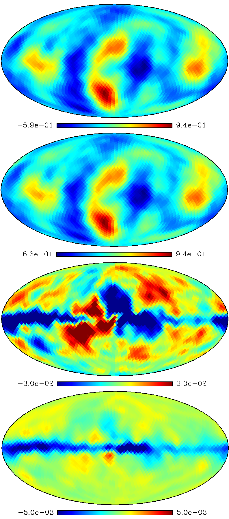
Figure 1: Top panel shows one random realization (seed = 100) of CMB E mode map at $N_{side}=16$ and Gaussian beam resolution of FWHM = $9^{\circ}$. The second panel shows the cleaned E mode map obtained following usual ILC algorithm (without using any prior information about the CMB covariance matrix) for the randomly chosen pure CMB E map shown in top panel. The third panel shows the difference between the second panel and the input CMB E mode map. A strong level of residuals is seen in the difference map. The bottom panel shows the mean of $1000$ difference maps formed by subtracting the pure CMB map from cleaned map following usual ILC method. The figure shows presence of residual contamination within the pixel range shown.

In this section, we discuss the results from the detailed Monte Carlo simulations in which we simulate $1000$ different set of input foreground contaminated CMB E mode maps at all COrE frequencies. We implement usual ILC and global ILC method to reconstruct the corresponding E mode CMB signal after properly minimizing the foregrounds in foreground model independent manner.The main scope of this section is to investigate in CMB E mode reconstruction over the large angular scales of the sky how significant are the the bias and errors in the cleaned CMB E mode map, corresponding CMB angular power spectrum obtained following usual ILC method and the global ILC method respectively.

4.1 Usual ILC Method

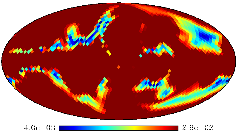
Figure 2: Figure showing standard deviation map computed from $1000$ difference maps obtained by subtracting the input CMB E maps from the corresponding cleaned E maps for usual ILC method. Poor reconstruction accuracy in usual ILC over large angular scales is readily concluded from this figure.

In the top panel of Fig. 1 we show the input E mode CMB map for a randomly chosen seed $100$. Corresponding cleaned E mode map obtained by using the usual ILC method is shown in the second panel of this figure. The color-scale of these subfigures are in $\mu K$ (thermodynamic) temperature. Although, both these subfigures look similar there are differences between the actual pixel distributions in each case, which may be inferred from the values indicated by the corresponding color scales. In the third panel of Fig. 1 we show the difference between the cleaned E map obtained by the usual ILC and the corresponding input E mode CMB map for the random seed $100$. Residuals of complex structure is prominently visible in the difference map in the plotted color scale showing significant residuals may exist of magnitude even as large as $0.03\mu K$ in the case of usual ILC method where no prior information about the CMB E mode covariance matrix is used. Using all $1000$ E mode cleaned maps obtained by the usual ILC method we estimate the mean difference map of cleaned and input CMB E mode signal. The resulting map is shown in the fourth panel of Fig. 1. The standard deviation map of residuals obtained from the simulations of usual ILC method shows very large errors which is shown in the in Fig. 2.

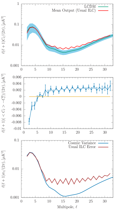
Figure 3: Top panel shows the mean cleaned E mode angular power spectrum obtained by following usual ILC method from $1000$ Monte Carlo simulations in red. The blue line shows the theoretical E mode angular power spectrum along with the theoretical cosmic variance induced error with light blue band. A negative bias at low multipoles and very strong positive bias (due to foreground residuals) are seen for multipoles starting $\ell\sim 7$. The middle panel shows the bias in the cleaned E mode power spectrum. Error-bars shown are applicable for the mean spectrum and are scaled versions (by $1/\sqrt{1000}$) of errors computed from the global ILC method. For $\ell\geq 8$ error bars are scaled additionally by a factor of $10$ to make them visible on the scales of the plot. The bottom panel shows a comparison of errors on cleaned E mode angular power spectrum (brown) and the theoretically computed cosmic variance induced error (blue). Inaccurate CMB E mode reconstruction following the usual ILC method is easily concluded from this plot.

Using $1000$ cleaned E mode angular spectra (after removing beam and pixel smoothing effects) from the cleaned E mode maps obtained by the usual ILC method we estimate a mean cleaned E mode angular power spectrum. The mean spectrum (in red) along with the input theoretical E mode angular power spectrum (in blue) is shown in the top panel of Fig. 3. The theoretical cosmic variance induced error is shown in this figure in light blue band. At the low multipoles $\ell\lesssim 4$ we see a negative bias in the cleaned power spectrum which has been also reported earlier for the CMB temperature anisotropy reconstruction following usual ILC method (Saha et al., 2006, 2008; Sudevan et al., 2017). The negative bias decreases with increase in $\ell$. Starting from $\ell\sim 7$ a strong residual foreground bias comes into existence in cleaned E mode spectrum obtained by this method. The bias in this multipole range becomes at least equal to and in several multipoles even more compared to the cosmic variance induced error. To emphasize the bias in the cleaned angular power spectrum is maximum around $\ell\sim 15$ where the expected CMB E mode signal is the weakest in the multipole range considered in this work. It is interesting to note here that the even multipoles has larger power due to residual foregrounds as compared to odd multipoles. The middle panel of this figure shows the bias in the cleaned E mode angular power spectrum at different multipole ranges. The error-bars shown in this panel are computed from the simulations of global ILC method, however, they are estimated for the mean spectrum obtained from $1000$ simulations, by multiplying the global ILC errors at different multipoles by the factor $1/\sqrt{1000}$. For $\ell\geq 8$ these scaled errors are multiplied by an additional factor of $10$ to make them visible on the vertical scale of this plot. A highly significant negative bias is observed in the usual ILC E mode angular spectrum at the low multipoles. A positive bias due to foreground residuals becomes very strong starting from $\ell=8$. The bottom panel of Fig. 3 compares the error-bars on the cleaned E mode angular spectrum with the cosmic variance error. Significantly larger errors compared to the cosmic variance prediction is observed for usual ILC reconstruction for the multipole starting from $\ell\sim 7$. It is interesting to note that the foreground residuals in the usual ILC method cause even multipoles to be more erroneous than the odd multipoles starting from $\ell\sim 9$. The bias for even multipoles in the cleaned EE mode angular power spectrum similarly is larger than the bias in neighbouring odd multipoles for $\ell\geq 7$ as seen from the second panel of Fig. 3.

4.2 Global ILC Method

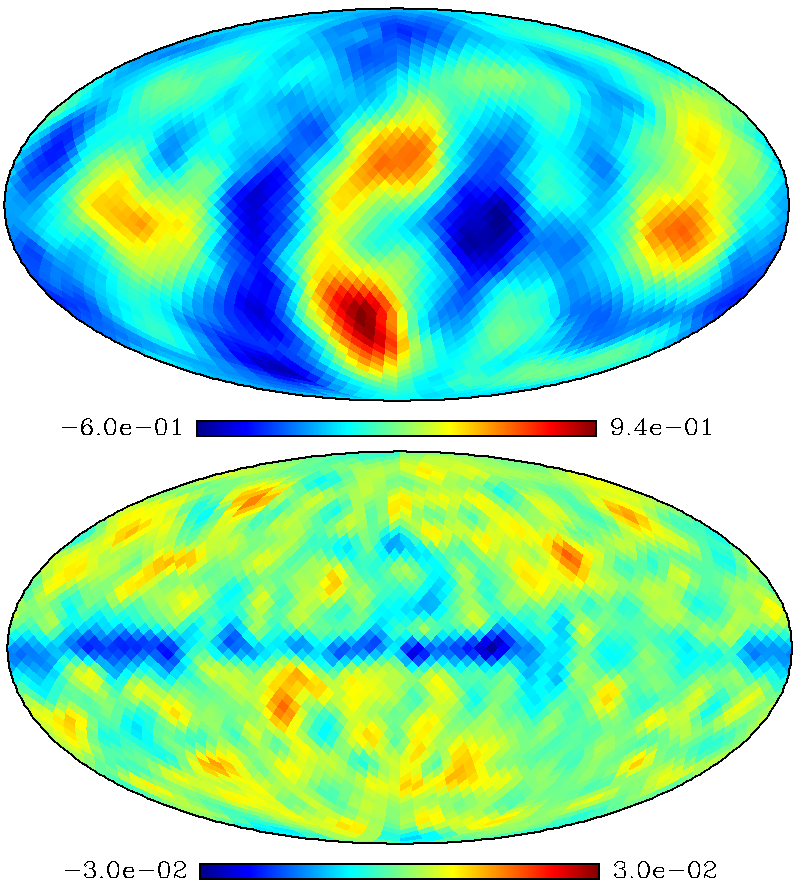
Figure 4: Top panel shows the reconstructed CMB E mode map following global ILC method using the prior knowledge of CMB E mode covariance matrix for the randomly chosen input CMB E mode map shown in top panel of Fig. 1. Both these figures agree well with each other. The bottom panel shows the difference between the top panel and the input CMB E mode map (top panel of Fig. 1) and hence represents residuals in global ILC method. Units for all maps are in $\mu K$ (thermodynamic).

In this section we discuss the results of Monte Carlo simulations of global ILC method, where we use prior information about the CMB E mode covariance matrix. Using each set of input frequency maps we estimate the CMB covariance matrix weighted matrix $A_{ij}$ using Eqn. 11 and compute the corresponding set of weights following Eqn. 8. We obtain a total of $1000$ cleaned E Mode CMB maps corresponding to all sets of input frequency maps. Apart from the CMB signal each of these cleaned maps contain small levels foreground residuals and minor level of detector noise. We show the input CMB E mode map for a randomly chosen seed ($100$) in top panel of Fig. 1. As is the case for this figure the typical pixel values for the large scale CMB E mode signal with the chosen beam resolution of $9^{\circ}$ of this work, lies within $\sim\pm 1\mu K$ . The top panel of Fig. 4 shows the reconstructed CMB E mode map using the global ILC method where prior information about the CMB E mode covariance matrix is used. Visually, both the input CMB E mode map (top panel of Fig. 1) and the cleaned map obtained by the global ILC method agree well with each other. In bottom panel of Fig. 4 we show the difference between the cleaned and the input E mode map. A small level of residuals is seen in this figure. The foreground residuals of this figure is clearly much smaller than the corresponding figure for the usual ILC case, shown in third panel of Fig. 1

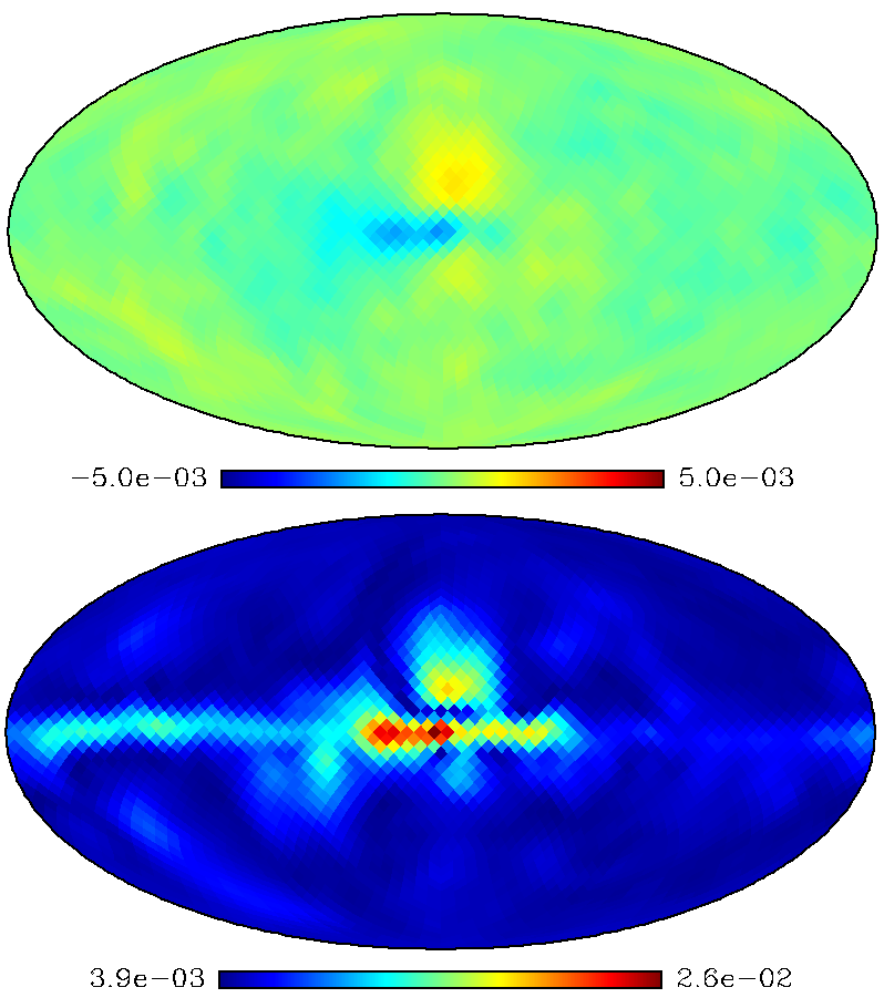
Figure 5: Top panel shows mean of $1000$ difference maps computed by subtracting input pure CMB E mode polarization maps from the cleaned E mode maps obtained by using global ILC method. The mean map shows average foreground residuals (which are $\lesssim 0.005\mu K$) present in the E mode CMB reconstruction method. The bottom panel shows the standard deviation map obtained from all $1000$ difference maps. Apart from the central and somewhat left side of the galactic plane the $1\sigma$ reconstruction error sky pixels are $\lesssim 0.004\mu K$.

To statistically assess the performance of the global ILC method to reconstruct the large scale cleaned E mode map we estimate the average foreground residuals in each of the cleaned maps by computing the mean difference map obtained by subtracting all $1000$ cleaned output and the corresponding input pure CMB E mode maps. The mean difference map is shown in the top panel of Fig. 5. The maximum of absolute pixel values of this map is well less than $0.005\mu K$ much less than typical value of pure CMB E mode standard deviation ($\sim 0.28\mu K$), indicating that the mean residual foregrounds in the cleaned maps are less than these estimates. The bottom panel of Fig. 5 shows the standard deviation map computed from all the difference maps. As seen from this map over most of the regions of the sky the reconstruction error is only $\sim 0.004\mu K$. Near the galactic plane the error tends to increase towards the left side and becomes maximum towards the galactic center where the maximum error becomes $0.026\mu K$.

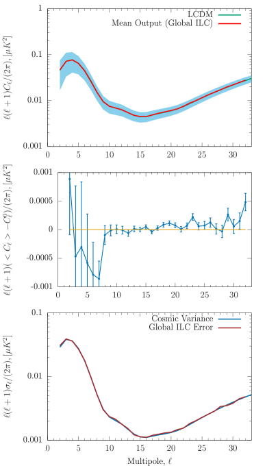
Figure 6: Top panel shows mean cleaned CMB E mode angular power spectrum (in red) obtained from global ILC method of this work using all $1000$ Monte Carlo simulations. The theoretical E mode angular power spectrum is shown in blue line but lies completely below the mean cleaned power spectrum on the scale of this plot. Theoretical cosmic variance induced error is shown in light blue band. The middle panel shows the difference between the mean cleaned and the theoretical E mode angular power spectrum in blue line. The error-bars shown are computed from Monte-Carlo simulations and applicable for the mean cleaned spectrum. The bottom panel shows the comparison of error on cleaned E power spectrum and theoretically estimated cosmic variance induced error. Both these estimates agree very well with each other indicating accurate CMB E mode reconstruction by global ILC method.

We estimate E mode CMB angular power spectrum from each of the $1000$ cleaned maps and remove the beam and pixel effects. We plot the average of all these spectra along with the input theoretical EE power spectrum used in all the Monte Carlo simulations to generate the CMB E mode map in top panel of Fig. 6. The mean CMB E mode spectrum (red) agrees very well with the theoretical spectrum (blue line), both of which are indistinguishable on the scale shown in this panel. It is specifically important to note that the global ILC method does not show presence of any positive bias, which may arise due to significant foreground residuals in the cleaned maps. Moreover, the average cleaned power spectrum does not show any indication of negative bias at the lowest multiples, which has been reported earlier for the case of CMB temperature anisotropy reconstruction following usual ILC method (Saha et al., 2006, 2008; Sudevan et al., 2017). This negative bias effect is also discussed later in Sec. 4.1 for the case of the usual ILC method in the context of CMB E mode reconstruction. The $1\sigma$ error band due to cosmic variance alone is also shown in this panel in blue. The middle panel of this figure shows the difference between the averaged cleaned E mode spectrum and the input theoretical power spectrum in blue line. The error-bars plotted in this figure are applicable for the averaged cleaned spectrum and is obtained by scaling the standard deviations of the cleaned angular spectrum obtained from the Monte Carlo simulations by the factor $\sqrt{1/1000}$. Clearly, the mean cleaned angular power spectrum does not deviate from the theoretical E mode power spectrum at the entire multipole range $2\leq\ell\leq 32$ showing no signature of bias in the cleaned power spectrum. The bottom panel of Fig. 6 shows comparison between the $1\sigma$ error-bars on the cleaned angular power spectrum at different multipoles estimated from Monte Carlo simulations (brown line) along with the theoretical estimates of cosmic variance induced error (in blue line). Both these estimates match very well with each other. This shows that the global ILC method reconstructs cleaned E mode angular power spectrum accurately as compared to the usual ILC method where the cleaned E mode CMB map and corresponding CMB angular power spectrum obtained from the later suffers from bias due to CMB-foregrounds chance correlation power dominant at large angular scales.

5 Role of Theoretical CMB E mode Covariance matrix in Global ILC Method

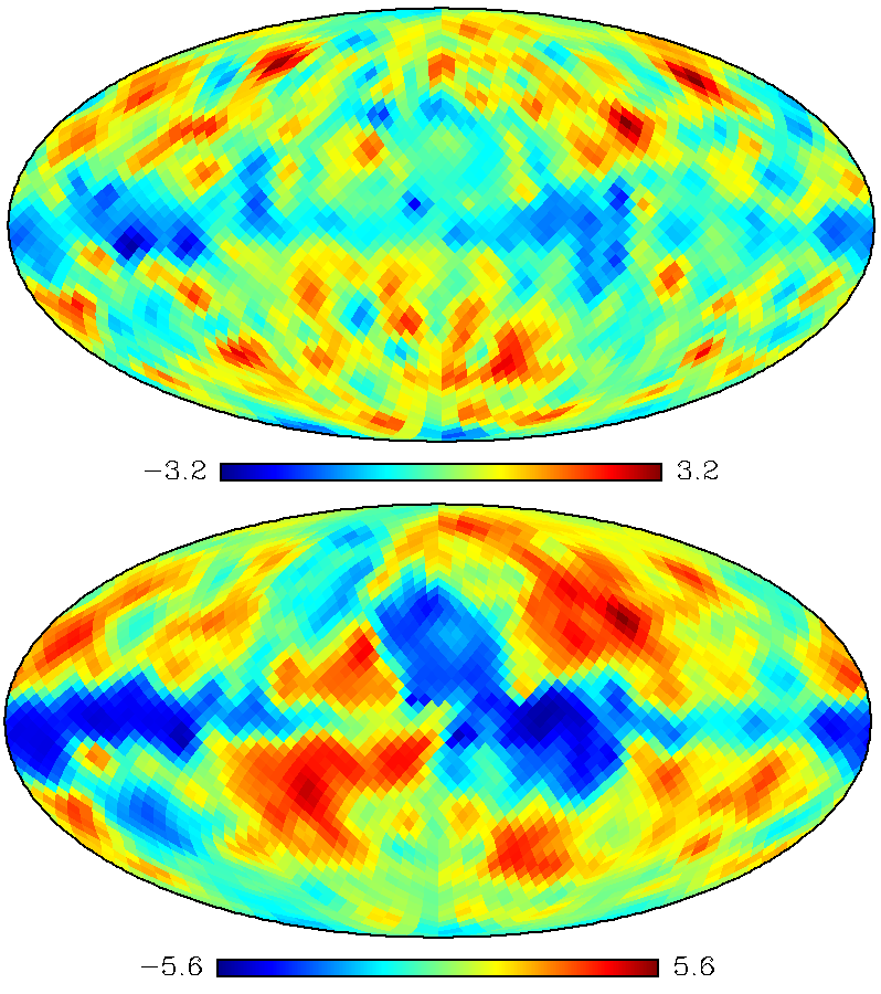
Figure 7: Top panel shows the significance of deviation of cleaned E mode map obtained following global ILC method from from the input pure CMB E mode map for a randomly chosen Monte Carlo simulation. The map represents cleaned output minus input CMB map weighted by the standard deviation map all from the global ILC method. The bottom panel shows the same for the usual ILC CMB E mode reconstruction, with standard deviation map used for weighting given also by the global ILC case. The larger significance of deviations of the bottom panel is caused by the stronger residuals present in the usual ILC case.

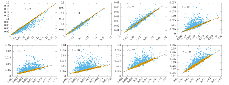
Figure 8: Figure showing scatter plot of E mode angular power spectra. The horizontal axis of each subplot denotes pure CMB E mode power spectrum for all $1000$ Monte Carlo simulations for different multipoles as indicated. Vertical coordinates of golden points are given by the cleaned angular power spectra obtained following global ILC method for all $1000$ cases for the respective multipoles. The vertical coordinates of blue points are given by the cleaned spectra from usual ILC method. The black line represents the straight line with slope unity. Presence of a negative bias at low multipoles and a positive bias at higher multipoles are evident for the reconstruction following usual ILC method. All axes represent $\ell(\ell+1)C^{E}_{\ell}/2\pi$ in unit of $\mu K^{2}$.

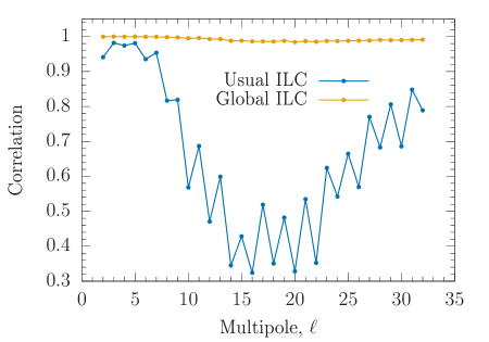
Figure 9: Figure showing strong correlation of CMB E mode angular power spectrum obtained by the global ILC method (in gold) with the input pure CMB E mode angular power spectrum for the multipole range $2\leq\ell\leq 32$. The blue line (with points) shows corresponding results for the usual ILC method. A poor correlation for the usual ILC method and excellent correlation for the global ILC method of this work are observed.

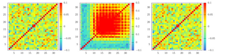
Figure 10: Figure showing the correlation matrix estimated using the angular power spectrum from $1000$ input CMB E mode maps (left panel), cleaned CMB E mode maps after removing foregrounds using usual ILC method (middle panel) and using global ILC method (right panel). We see the correlation matrix estimated from global ILC method is consistent with the input E mode CMB maps. For the usual ILC method a strong correlation between multipoles due to residual foreground contaminations is visible.

The chance correlations between CMB and non-CMB E mode signals is a significant source of concern for application of ILC method towards cleaned CMB E mode signal estimation, specifically over the large angular scales over the sky. The global ILC method provides a pathway to accurately reconstruct the CMB signal at the low multipole regions using prior information about the CMB covariance matrix, so that the cleaned E mode map has a covariance structure consistent with the expected theory of the CMB angular power spectrum. Using the theoretical CMB covariance matrix model the global ILC method effectively suppresses the CMB and non-CMB components chance correlation power at the low multipoles through Eqn. 12 by weighting down the chance-correlation fluctuations in $\sigma^{ij}_{\ell}$ by the inverse of E mode theoretical power spectrum. This leads to significantly improved estimation of both E mode cleaned map and its angular power spectrum by the global ILC method compared to the usual ILC case.

In top panel of Fig. 7 we show difference of a randomly chosen cleaned E map (corresponding to the seed $100$) of global ILC method and input CMB E map after weighting each pixel value by the standard deviation map obtained in the same method (shown in bottom panel of Fig. 5). The pixel values of this weighted difference map represents significance of deviations, which lie within $\pm 3.2\sigma$, indicating no significant bias present in the cleaned E mode map obtained by the global ILC method. In the bottom panel of Fig. 7 we show the difference map of usual ILC and the input CMB E mode map (for the same seed $100$) weighting each pixel by the standard deviation map of global ILC method. The larger pixel values of the bottom panel of Fig. 7 compared to the top panel represents a significant bias present in the reconstructed E mode map by the usual ILC method.

Suppression of chance correlation power in the global ILC method results in accurate estimation of CMB E mode angular power spectrum. In Fig. 8 we present a scatter plot of E mode angular power spectra to represent this general feature for only some representative multipoles at different ranges as indicated in the figure. For each sub-plot of this figure the horizontal axis represents the values of the randomly generated pure CMB E mode angular power spectrum for the specific multipole indicated in the sub-plot. The vertical axis of a subplot represents the cleaned power spectra values for the corresponding multipole obtained by either global ILC method (golden points) or by usual ILC method (blue points). The black-line in sub-plot shows the straight line with unit slope corresponding maximal correlation between the input and cleaned CMB E mode spectrum for any of the two methods. Two interesting features of this figure require some emphasis. First, at the low multipoles $\ell=2$ or $3$ the recovered angular spectrum tend to have a value lower than the input E mode CMB power spectrum for the blue points. This indicates presence of a negative bias at the low multipoles in the usual ILC method. The results for the usual ILC method is completely opposite for the multipoles starting from $\ell\sim 7$ where more and more blue points tend to lie above the black line. This implies that a strong positive bias due to foreground residuals because of presence of the chance-correlations comes into picture in the usual ILC method. Some blue points specifically for multipole starting $\ell=10$ of this plot lie very far away and above the black lines. This further indicates unsatisfactory performance of usual ILC method to estimate the E mode angular power spectrum at low resolution. The golden points traces the black-lines closely for all the multipoles denoting tight correlation between the cleaned and the input CMB E mode angular power spectra. This indicates a very desirable property of a CMB reconstruction method achieved by the global ILC method of this work, namely, the cleaned angular power spectrum must be – very strongly correlated with the pure input CMB E mode spectrum, for an accurate reconstruction of CMB E mode angular power spectrum. We show in Fig. 9 correlation of cleaned E mode angular power spectra with the input pure CMB spectrum for different multipoles for the usual ILC and global ILC foreground removal method. The usual ILC spectra becomes very weakly correlated with the input CMB E mode spectrum for the entire multipole range $2\leq\ell\leq 32$. At $\ell=16$ correlation value for usual ILC drops to merely $32$%. For the reconstruction following global ILC method the minimum correlation is very large $98.4$%, which occurs for $\ell=20$. The average correlations for the global method for the entire multipole range is found to be as large as $99.1$%.

Each of the two methods – usual ILC and the global ILC, produces a set of $1000$ cleaned CMB E mode angular power spectra. We estimate two correlation matrices of the cleaned spectra corresponding to these two sets. The middle and last panel of Fig 10 shows respectively the correlation matrix for the usual ILC and the global ILC method. The figure in the middle panel contains large non-diagonal elements (as large as $50$%) which indicates that the usual ILC cleaned spectra contain strong foreground contamination. The first panel of Fig. 10 shows the correlation matrix for the input E mode angular power spectra estimated from the $1000$ pure CMB E mode maps. Both the first and third panel agree very well with each other. From Fig. 10 we, therefore, conclude that the cleaned spectra estimated from the global ILC method is highly accurate and does not possess any significant foreground residuals.

6 Discussion and Conclusion

An accurate measurement of CMB E mode polarization signal over large angular scales can be used to constrain the physics of reionization and the decoupling epoch. The CMB E mode signal over the large angular scales helps to remove degeneracy between the amplitude of scalar fluctuations and optical depth to the reionization epoch. Since the large scale CMB E mode polarization is a weak signal, the problem of reconstructing a cleaned E mode CMB map by removing foregrounds becomes a complex task. Therefore, one requires to carefully device an accurate reconstruction technique so that the cleaned signal can be reliably used for cosmological analysis.

In this article, we, for the first time, performed a detailed investigation of reconstruction of CMB E mode signal over large angular scales following ILC method by removing astrophysical foregrounds using simulated observations of first $15$ frequency bands of future generation COrE satellite mission. We implemented usual ILC method and an improved and accurate global ILC method which uses the prior information of CMB E mode covariance matrix over large angular scales of the sky. Our results show that the global ILC method can reconstruct the weak CMB E mode signal accurately over large angular scales in contrast to the usual ILC method.

The empirical data covariance matrix in the usual ILC method, specifically for CMB E signal reconstruction over large angular scales of the sky, contains a chance correlation power between the CMB and non-CMB components (e.g., foregrounds). This chance correlation power is very strong at large angular scales over the sky due to lower number of available independent modes on these scales. We have shown in this work, this chance correlation power strongly biases the cleaned E map and the estimated angular power spectrum in the usual ILC method. The chance correlation power merely behaves as random noise and effectively increases rank of the empirical frequency-frequency data covariance matrix leading to large foreground residuals in the cleaned E maps. The strong foreground residuals present in the cleaned E map implies that the covariance matrix of the cleaned map is far from the underlying CMB E mode covariance matrix. In the new global ILC method, we overcome the problem of usual ILC method by incorporating the theoretical CMB E mode covariance matrix in the cleaning algorithm. This causes the cleaned E mode CMB map obtained by using global ILC method to have a covariance structure compatible to the underlying theoretical E mode angular power spectrum. Using the underlying covariance matrix in our method, therefore, effectively suppresses the chance correlation power and results in the accurate estimation of CMB E mode signal and the full-sky angular power spectrum over the large angular scales.

By doing detailed Monte Carlo simulations we show that there exists a large error in the usual ILC cleaned maps due to the CMB-foreground chance correlation power which dominates at large angular scales. The error is more than $0.026$ $\mu K$ for almost all regions of the sky. The cleaned power spectrum estimated from the cleaned maps obtained following foreground removal using usual ILC method is biased strongly both due to a negative bias at the low multipoles and positive bias at higher multipoles. The error bars on the cleaned E mode power spectrum are in general way larger than the cosmic variance prediction for the multipole range $\ell\geq 7$ of this analysis. The new method shows significantly reduced error due to residual foregrounds in the galactic plane. The error in the reconstruction of the cleaned E mode map, due to foreground residuals in the cleaned map, is somewhat large only in the galactic central region where $1\sigma$ error is given by $0.026$ $\mu K$ only at a single pixel . The mean cleaned E mode spectrum from the simulations of the global ILC method does not show presence of any bias. The $1\sigma$ errors of the E mode angular power spectrum agree very well the cosmic-variance induced error alone.

Not only the cleaned E maps obtained by using the usual ILC method show presence of significant error the angular power spectra estimated from these maps show strong correlation between different multipoles indicating presence of foreground residuals in the cleaned angular power spectra. A strong positive correlation of about 50% for either $\ell$ or $\ell^{\prime}$ larger than $10$ is obtained for the usual ILC case. At lower multipoles pair, the effect of negative bias due to CMB-foreground chance correlations leads to a weak negative correlation of about $10$% in the $\ell-\ell^{\prime}$ matrix. For the cleaned E mode angular power spectra obtained using the global ILC method corresponding correlation structure is manifest only along the diagonal elements of the correlation matrix which agree excellently with the correlation matrix obtained from the simulations of pure CMB E mode angular power spectra. This indicates an accurate CMB E mode reconstruction following the global ILC method.

An interesting statistical feature of the cleaned global ILC E mode angular power spectra is that the cleaned $C^{E}_{\ell}$ remains tightly correlated with the corresponding input pure CMB $C^{E}_{\ell}$ for all multipoles $2\leq\ell\leq 32$. This is particularly very advantageous for the multipole range $10\leq\ell\leq 25$ where pure E mode $C^{E}_{\ell}(\ell+1)\ell/2\pi$ is very weak. Presence of strongly outlying (erroneous) cleaned angular power spectrum is a general feature for the usual ILC case. Such outliers are entirely absent for the reconstruction performed following global ILC method.

Like the usual ILC method, the global ILC CMB E mode reconstruction does not get affected by the any modelling uncertainties in the polarized foreground components. The global ILC method effectively suppresses the CMB-foreground chance correlation power at large angular scales and thereby provides an accurate reconstruction of weak CMB E mode map and its angular power spectrum. The method can be extended further to obtain a cleaned B mode CMB map and its angular power spectrum. This will be investigated in a future publication.

7 Acknowledgement

We use publicly available HEALPix package (Górski et al., 2005) for the analysis of this work (http://healpix.sourceforge.net).

References

- Basak & Delabrouille (2012) Basak, S., & Delabrouille, J. 2012, MNRAS, 419, 1163
- Basak & Delabrouille (2013) —. 2013,MNRAS, 435, 18
- Basko & Polnarev (1980) Basko, M. M., & Polnarev, A. G. 1980, Soviet Ast., 24, 268
- Bennett et al. (1992) Bennett, C. L., Smoot, G. F., Hinshaw, G., et al. 1992, ApJL, 396, L7
- Bennett et al. (2003) Bennett, C. L., Hill, R. S., Hinshaw, G., et al. 2003, ApJS, 148, 97
- Bouchet & Gispert (1999) Bouchet, F. R., & Gispert, R. 1999,New Astron , 4, 443
- Burigana et al. (2008) Burigana, C., Popa, L. A., Salvaterra, R., et al. 2008, MNRAS, 385, 404
- Delabrouille et al. (2018) Delabrouille, J., de Bernardis, P., Bouchet, F., et al. 2018, Journal of Cosmology and Astroparticle Physics, 2018, 014
- Eriksen et al. (2008a) Eriksen, H. K., Dickinson, C., Jewell, J. B., et al. 2008a, ApJL, 672, L87
- Eriksen et al. (2008b) Eriksen, H. K., Jewell, J. B., Dickinson, C., et al. 2008b, ApJ, 676, 10
- Eriksen et al. (2004) Eriksen, H. K., O’Dwyer, I. J., Jewell, J. B., et al. 2004, ApJs, 155, 227
- Eriksen et al. (2006) Eriksen, H. K., Dickinson, C., Lawrence, C. R., et al. 2006, ApJ, 641, 665
- Gold et al. (2011) Gold, B., Odegard, N., Weiland, J. L., et al. 2011, ApJS, 192, 15
- Górski et al. (2005) Górski, K. M., Hivon, E., Banday, A. J., et al. 2005, ApJ, 622, 759
- Hanany et al. (2019) Hanany, S., Alvarez, M., Artis, E., et al. 2019, arXiv e-prints, arXiv:1902.10541
- Knox & Song (2002) Knox, L., & Song, Y.-S. 2002, Phys. Rev. Lett., 89, 011303
- Lewis (2003) Lewis, A. 2003, Phys. Rev. D, 68, 083509
- Lewis et al. (2002) Lewis, A., Challinor, A., & Turok, N. 2002, Phys. Rev. D, 65, 023505
- Mather et al. (1994) Mather, J. C., Cheng, E. S., Cottingham, D. A., et al. 1994, ApJ, 420, 439
- Matsumura et al. (2014) Matsumura, T., Akiba, Y., Borrill, J., et al. 2014, Journal of Low Temperature Physics, 176, 733
- Page et al. (2007) Page, L., Hinshaw, G., Komatsu, E., et al. 2007, ApJS, 170, 335
- Penrose (1955) Penrose, R. 1955, Proceedings of the Cambridge Philosophical Society, 51, 406
- Planck Collaboration et al. (2016a) Planck Collaboration, Adam, R., Ade, P. A. R., et al. 2016a, A&A, 594, A9
- Planck Collaboration et al. (2016b) Planck Collaboration, Aghanim, N., Ashdown, M., et al. 2016b, A&A, 596, A107
- Planck Collaboration et al. (2018a) Planck Collaboration, Akrami, Y., Ashdown, M., et al. 2018a, arXiv e-prints, arXiv:1807.06208
- Planck Collaboration et al. (2018b) Planck Collaboration, Aghanim, N., Akrami, Y., et al. 2018b, arXiv e-prints, arXiv:1807.06209
- Rees (1968) Rees, M. J. 1968, ApJL, 153, L1
- Remazeilles et al. (2011) Remazeilles, M., Delabrouille, J., & Cardoso, J.-F. 2011, MNRAS, 418, 467
- Remazeilles et al. (2018a) Remazeilles, M., Dickinson, C., Eriksen, H. K., & Wehus, I. K. 2018a, MNRAS, 474, 3889
- Remazeilles et al. (2018b) Remazeilles, M., Banday, A. J., Baccigalupi, C., et al. 2018b, Journal of Cosmology and Astroparticle Physics, 2018, 023
- Saha (2011) Saha, R. 2011, ApJL, 739, L56
- Saha & Aluri (2016) Saha, R., & Aluri, P. K. 2016, ApJ, 829, 113
- Saha et al. (2006) Saha, R., Jain, P., & Souradeep, T. 2006, ApJL, 645, L89
- Saha et al. (2008) Saha, R., Prunet, S., Jain, P., & Souradeep, T. 2008, Phys. Rev. D, 78, 023003
- Spergel & Zaldarriaga (1997) Spergel, D. N., & Zaldarriaga, M. 1997, Phys. Rev. Lett., 79, 2180
- Sudevan et al. (2017) Sudevan, V., Aluri, P. K., Yadav, S. K., Saha, R., & Souradeep, T. 2017, ApJ, 842, 62
- Sudevan & Saha (2018a) Sudevan, V., & Saha, R. 2018a, ApJ, 867, 74
- Sudevan & Saha (2018b) —. 2018b, arXiv e-prints, arXiv:1810.08872
- Sudevan & Saha (2020) —. 2020, arXiv e-prints, arXiv:2001.02849
- Sugai et al. (2020) Sugai, H., Ade, P. A. R., Akiba, Y., et al. 2020, arXiv e-prints, arXiv:2001.01724
- Tegmark & Efstathiou (1996) Tegmark, M., & Efstathiou, G. 1996, MNRAS, 281, 1297
- Watts et al. (2019) Watts, D. J., Addison, G. E., Bennett, C. L., & Weiland , J. L. 2019, arXiv e-prints, arXiv:1910.00590
- Zaldarriaga & Seljak (1998) Zaldarriaga, M., & Seljak, U. 1998, Phys. Rev. D, 58, 023003