On Biased Random Walks, Corrupted Intervals, and Learning Under Adversarial Design

Abstract

We tackle some fundamental problems in probability theory on corrupted random processes on the integer line. We analyze when a biased random walk is expected to reach its bottommost point and when intervals of integer points can be detected under a natural model of noise. We apply these results to problems in learning thresholds and intervals under a new model for learning under adversarial design.

1 Introduction and previous work

In this paper, we tackle some fundamental questions in probability theory, in particular by looking at “corrupted" processes on the integer line. We can view biased random walks as instances of such a corrupted process, where the random walk is “supposed to” go up, but is occasionally corrupted and goes down. Among our results is an analysis of when such random walk is expected to hit its bottommost point. In the case of intervals, points within and outside the interval are labeled accordingly, but again, we analyze the case when such labels are corrupted and show when the interval can be recovered.

While these are the main results and are of clear independent interest, we also connect them to problems in learning under adversarial design. Our results are also related to the classical, purely analytical mathematical notion of upcrossing (Gofer, 2014; Koolen and Vovk, 2014; Teichmann, 2015). In the case of the integer line processes we find tight estimators on the extremal upcrossings with optimal lower bounds and in the case of the interval we find tight cutoffs for the minimum magnitude of substantial, or true-upcrossings (corresponding to those intervals that can be recovered) as distinguished from transient, or pseudo-upcrossings which are fundamentally indistinguishable from variations which arise merely as an artifact of minor random noise.

In Section 2, we give both upper and exact bounds on the last time an up-biased random walk will hit its bottommost point. In Section 3 we give results of a similar flavor for corrupted samples from an interval on the integer line. Then, in Section 4, we extend adversarial design to the machine learning and show how our results on corrupted processes give learnability results for adversarial design.

1.1 Random walks

Much of the literature on random walks on the line focuses on the unbiased case, where at each time-step, a random walk is equally likely to go up as down. Quantities such as the expected distance to the origin are often analyzed, as well as the observation that every point will be eventually reached by such a walk, which gives rise to phenomena such as “gambler’s ruin” (Harik et al., 1999) and the existence of a few “favorite sites” of a random walk (Toth, 2001),.

1.2 Learning under adversarial design

The celebrated Probably Approximately Correct (PAC) model (Valiant, 1984) has been enormously influential in setting the learning-theoretic agenda over the past thirty years. Indeed, this model has laid the foundation for a clean and elegant theory while retaining some measure of empirical plausibility. Regarding the latter criterion, numerous results have aimed at whittling away at the model’s initially somewhat restrictive formulation. The original requirement of clean labels was relaxed to encompass a benign type of label noise (Angluin and Laird, 1987; Kearns, 1998), as well as considerably more adversarial noise models (Kearns and Schapire, 1994; Kearns et al., 1994). Similarly, the i.i.d. sampling assumption — which early learning theory papers often took pains to apologize for — has by now been subsumed by far less restrictive mixing conditions (Gamarnik, 2003; Karandikar and Vidyasagar, 2002; London et al., 2012, 2013; Mohri and Rostamizadeh, 2008, 2010; Rostamizadeh and Mohri, 2007; Shalizi and Kontorovich, 2013; Steinwart and Christmann, 2009; Steinwart et al., 2009; Zou et al., 2014). In the online learning model (Cesa-Bianchi and Lugosi, 2006), one dispenses with a sampling distribution entirely, and instead assumes an adversarially chosen sequence of labeled examples. Due to this model’s worst-case nature, one can only prove regret bounds as opposed to absolute error estimates. Many related xresearch directions also include aspects of online learning and non-stationary processes (Agarwal and Duchi, 2013; Anava et al., 2013; Audiffren and Ralaivola, 2015; Zimin and Lampert, 2017; Kuznetsov and Mohri, 2015).

In this section, we propose a distribution-less variant of learning akin to the adversarial design framework for regression. Unlike the online setting, training data is provided in batch and we use its structure to draw conclusions about the range of possible target hypotheses. In this sense, our learning model conceptually resembles the so-called “algorithmic luckiness” framework (Herbrich and Williamson, 2002; Shawe-Taylor et al., 1998), where the generalization bound depends on the empirical configuration of the training sample (such as it having a large margin). The salient difference is that the former requires i.i.d. samples, while we allow an arbitrary set of points. Our model attempts to capture situations in which the training data is sufficiently informative so as to pick out only very few potential candidate hypotheses. If, furthermore, all of these candidates are “close” in some metric, it stands to reason that all of them are in fact close to the target concept in that metric.

Linear regression provides a canonical example of this situation (worked out in detail in Section 4.1). Indeed, when the response variable $y=\boldsymbol{\mathrm{w}}^{\intercal}\boldsymbol{\mathrm{x}}$ is a noiseless linear function of the $d$-dimensional predictor variables $\boldsymbol{\mathrm{x}}$, it suffices to observe $d$ labeled points in general position in order to recover $\boldsymbol{\mathrm{w}}$ exactly. When the observations are perturbed by additive noise ($y=\boldsymbol{\mathrm{w}}^{\intercal}\boldsymbol{\mathrm{x}}+\xi$), it will be possible to recover $\boldsymbol{\mathrm{w}}$ up to an error that depends on the configuration of the training points as well as the magnitude of the noise (essentially, a signal to noise ratio).

2 Biased random walks

Given a random walk on the integer line with upward and downward step probabilities of $p>1/2$ and $q=1-p$, respectively, let $T$ be the last time the bottommost point is visited. Formally, let $Z_{1},Z_{2},\ldots$ be independent random variables taking value $1$ with probability $p$ and $-1$ with probability $q=1-p$. Let $S_{0}=0$ and $S_{t}=\sum_{i=1}^{t}Z_{i}$. The bottommost point is a random variable $B=\min_{t\geq 0}\{S_{t}\}$, and the last time the bottommost value $B$ is visited is $T=\max\{t\geq 0:\ S_{t}=B\}$.

We would like to understand $\mathbb{P}(T\geq t)$. We will find both the probability generating function and the moment generating function of $T$. We will also find a closed-form expression for $P(T\geq t)$ in terms of the Gaussian hypergeometric function and an asymptotic expression in terms of the Lerch function. We recall these function below. The asymptotic behavior depends on two variables, and because of this we will find two elementary upper bounds for when one or the other variable is dominating the behavior and also one lower bound in elementary terms to indicate the basic level of precision of these estimates.

2.1 An upper bound on $\mathbb{P}(T\geq t)$

First, we show that $\mathbb{P}(T\geq t)=O\left((4pq)^{t/2}\right)$; in fact, the implied constant may be computed explicitly.

Theorem 1.

Let $T$ be the last time the bottommost point is visited in a random walk with “up" bias $p$ (and $q=1-p$), then

$$\mathbb{P}(T\geq t)\leq(1+\sqrt{2})(4pq)^{t/2}.$$

We will prove this using the moment generating function which is calculated in Lemma 2.

Lemma 2.

The moment generating function of $T$ is given by

$$\mathbb{E}[e^{sT}]=\frac{2(p-q)}{1+\sqrt{1-4pqe^{2s}}-2qe^{s}},\qquad 0\leq s\leq\frac{1}{2}\log\frac{1}{4pq},$$

and in particular,

$$\mathbb{E}[T]=\frac{q(3-4q)}{(p-q)^{2}}.$$

Much of the combinatorics of what follows is closely related to the Catalan numbers:

$$C_{n}=\frac{1}{n+1}\binom{2n}{n},\qquad n=0,1,2,\dots$$

and their generating function is (Koshy, 2009, pp. 122)

$$C(x)=\sum^{\infty}_{n=0}C_{n}x^{n}=\frac{1-\sqrt{1-4x}}{2x}.$$

and the closely related central binomial coefficient generating function is (Koshy, 2009, pp. 27-28)

$$\sum^{\infty}_{n=0}(n+1)C_{n}x^{n}=\sum^{\infty}_{n=0}\binom{2n}{n}x^{n} =\frac{1}{\sqrt{1-4x}}.$$

Proof of Lemma 2.

It will be instructive to actually start by calculating directly the first two moments, $\mu_{1}:=\mathbb{E}[T]$ and $\mu_{2}:=\mathbb{E}[T^{2}]$ of $T$. If on the first step, the drunkard moves upward and never visits $0$ again (which happens with probability $p-q$), then $T=0$. If he moves upward and returns to $0$ for the first time in $2k$ steps, which happens with probability

$$p\binom{2k-2}{k-1}(pq)^{k-1}q/k=C_{k-1}(pq)^{k},$$

then the conditional expectation of $T$ is $2k+\mu_{1}$. If on the first step he moves down, the conditional expectation is $\mu_{1}+1$. Hence:

$$\mu_{1} = (p-q)\cdot 0+pq\sum_{k=1}^{\infty}C_{k-1}(pq)^{k-1}(\mu_{1}+2k)+\ q\cdot(\mu_{1}+1),$$

so that

$$p\mu_{1} = \mu_{1}pq\sum_{k=0}^{\infty}C_{k}(pq)^{k}+2pq\sum_{k=0}^{\infty}(k+1)C_{k}(pq)^{k}+q=\frac{1}{2}\mu_{1}\left(1-\sqrt{1-4pq}\right)+2\frac{pq}{\sqrt{1-4pq}}+q,$$

whence

$$\mu_{1}=\frac{q(3-4q)}{(p-q)^{2}}.$$

Let us now calculate $\mu_{2}:=\mathbb{E}[T^{2}]$. By reasoning similar to above,

$$\mu_{2} = (p-q)\cdot 0^{2}+\sum_{k=1}^{\infty}\frac{\binom{2k-2}{k-1}}{k}(pq)^{k}\cdot\mathbb{E}[(T+2k)^{2}]+\ q\cdot\mathbb{E}[(T+1)^{2}]$$

$$= q\mu_{2}+4\sum_{k=1}^{\infty}\binom{2k-2}{k-1}(pq)^{k}x+\ 4\sum_{k=1}^{\infty}k\binom{2k-2}{k-1}(pq)^{k}+q\mu_{2}+2qx+q,$$

whence

$$\mu_{2}=\frac{q(1-8p+28p^{2}-16p^{3})}{(p-q)^{4}}.$$

In this manner we can compute the moment generating function of $T$:

$$\mathbb{E}[e^{sT}] = (p-q)\cdot 1+\sum_{k=1}^{\infty}C_{k}(pq)^{k}\cdot\mathbb{E}[e^{s(T+2k)}]+\ q\cdot\mathbb{E}[e^{s(T+1)}].$$

Thus,

$$\mathbb{E}[e^{sT}]=\frac{2(p-q)}{1+\sqrt{1-4pqe^{2s}}-2qe^{s}},\qquad 0\leq s\leq\frac{1}{2}\log\frac{1}{4pq}.$$

∎

Now we are ready to prove the main theorem.

Proof of Theorem 1. By Markov’s inequality,

$$\mathbb{P}(T\geq t) \leq \frac{2(p-q)e^{-st}}{1+\sqrt{1-4pqe^{2s}}-2qe^{s}},\quad\text{for all}\quad 0\leq s\leq\frac{1}{2}\log\frac{1}{4pq}.$$

The choice $s=\frac{1}{2}\log\frac{1}{4pq}$ yields

$$\mathbb{P}(T\geq t)\quad\leq\quad\frac{2(p-q)(4pq)^{t/2}}{1-\sqrt{q/p}}\quad=\quad 2\sqrt{p}(\sqrt{p}+\sqrt{q})(4pq)^{t/2}.$$

A routine calculation gives

$$\max_{x\in[1/2,1]}\sqrt{x}(\sqrt{x}+\sqrt{1-x})=(1+\sqrt{2})/2.$$

Thus

$$\mathbb{P}(T\geq t)\leq(1+\sqrt{2})(4pq)^{t/2},$$

which completes the proof. $\Box$

Because this random walk problem is so natural and of independent interest, in the following section we give an exact computation for $\mathbb{P}(T\geq t)$.

2.2 Exact analysis for $\mathbb{P}(T\geq t)$

Here, we calculate an exact expression for $\mathbb{P}(T\geq t)$ in terms of the Gaussian hypergeometric function (Bateman, 1981) ${}_{2}F_{1}$, which is defined for $|x|<1$ by

$${}_{2}F_{1}(a,b;c;x)=\sum^{\infty}_{n=0}\frac{(a)_{n}(b)_{n}}{(c)_{n}}\frac{x^{n}}{n!},$$

where

$$(\alpha)_{n}=\begin{cases}1,&\qquad n=0,\\ \alpha(\alpha+1)\cdots(\alpha+n-1),&\qquad n>0,\end{cases}$$

is the rising Pochhammer symbol. For convenience we let $\tau=\left\lfloor{\frac{t+1}{2}}\right\rfloor$.

It is elementary to check that

$$C_{n}=C_{k}\frac{(k+(1/2))_{n-k}}{(k+2)_{n-k}}4^{n-k},\qquad n>k\geq 0.$$ (1)

So

$$\sum^{k-1}_{n=0}C_{n}x^{n}-C(x) =-\sum^{\infty}_{n=k}C_{n}x^{n}=-x^{k}C_{k}\sum^{\infty}_{n=k}\frac{(k+(1/2))_{n-k}}{(k+2)_{n-k}}4^{n-k}x^{n-k}.$$

Therefore

$$\sum^{k-1}_{n=0}C_{n}x^{n}=-x^{k}C_{k}\cdot{}_{2}F_{1}(1,k+(1/2);k+2;4x)+\frac{1-\sqrt{1-4x}}{2x}.$$ (2)

It will be convenient to view the random variable $T$ of Lemma 1 from a slightly different viewpoint. Consider the following random walk in $\mathbb{Z}^{2}$. Begin at the origin. If at $(a,b)$, then with probability $p>1/2$ on the next step move to $(a+1,b-1)$, and with probability $q=1-p$ move to $(a+1,b+1)$. Let $f(k,l)$ for $0\leq l\leq k$ be the probability that both $l$ is the absolute maximum second argument reached in the course of the walk and that, among those points with maximum second argument, $k$ is the maximum value of the first argument (thus $T=k$). So informally $f(k,l)$ is the probability that $(k,l)$ is the last highest point of the walk. Conditioning on the first step, we get

$$f(k,l)=qf(k-1,l-1)+pf(k-1,l+1),\qquad(k,l)\neq(0,0).$$ (3)

Consider the generating function

$$F(x,y)=\sum^{k}_{l=0}f(k,l)x^{k}y^{l}.$$

We recall (see, e.g., the “gambler’s ruin” analysis in Levin et al. (2017, Section 17.3.1)) that the probability of the $(p-q)$-biased random walk never returning to $0$ is $p-q$, whence

$$f(0,0)=p-q.$$ (4)

Theorem 3.

We have

$$\mathbb{P}(T\geq t)= (p-q)p(pq)^{\tau}C_{\tau}\left({}_{2}F_{1}(1,\tau+(1/2);\tau+2;4pq)+4pq\frac{\tau+(1/2)}{\tau+2}{}_{2}F_{1}(2,\tau+(3/2);\tau+3;4pq)\right).$$

Proof.

We recall that the Catalan number $C_{n}$ may be interpreted as the number of walks in our scheme ending at $(0,2n)$ and never passing below the starting point. With this interpretation, it is easy to see from Equation 4 that

$$\sum^{\infty}_{k=0}f(k,0)x^{k}=(p-q)C\left(pqx^{2}\right).$$ (5)

Thus using Equations 3 and 5 we get

$$F(x,y) =f(0,0)+\sum_{k=1}^{\infty}\sum_{l=0}^{k}f(k,l)x^{k}y^{l}$$

$$=f(0,0)+q\sum_{k=1}^{\infty}\sum_{l=1}^{k}f(k-1,l-1)x^{k}y^{l}+p\sum_{k=1}^{\infty}\sum_{l=0}^{k}f(k-1,l+1)x^{k}y^{l}$$

$$=f(0,0)+qxyF(x,y)+p\frac{x}{y}\sum_{k=1}^{\infty}\sum_{l=0}^{k}f(k-1,l+1)x^{k-1}y^{l+1}$$

$$=f(0,0)+qxyF(x,y)+p\frac{x}{y}\sum_{l=1}^{k}f(k,l)x^{k}y^{l}$$

$$=f(0,0)+qxyF(x,y)+p\frac{x}{y}F(x,y)-p(p-q)\frac{x}{y}C(pqx^{2}).$$

Therefore

$$F(x,y)=\frac{p-q}{1-qxy-\frac{px}{y}}\left(1-\frac{px}{y}C\left(pqx^{2}\right)\right).$$

In particular,

$$F(x,1)(1-x) =(p-q)(1-pxC(pqx^{2})),$$

so that

$$F(x,1) =(p-q)\left(1-pxC\left(pqx^{2}\right)\right)\left(\sum_{i\geq 0}x^{i}\right),$$

which upon multiplying out becomes

$$F(x,1) =(p-q)+(p-q)\sum_{k\geq 1}\left(1-p\sum_{0\leq n\leq\left\lfloor{\frac{k-1}{2}}\right\rfloor}C_{n}(pq)^{n}\right)x^{k}.$$ (6)

Let $F(k)$, $k\geq 0$, be the coefficients of the power series expansion of $F(x,1)$ as $F(x,1)=\sum_{k\geq 0}F(k)x^{k}$. Then $F(0)=p-q$, and from (6), (1) and (2) we get for $k\geq 1$,

$$F(2k)=F(2k-1) =(p-q)\left(1-p\sum_{0\leq n\leq k-1}C_{n}(pq)^{n}\right)$$

$$=(p-q)\left(1+p(pq)^{k}C_{k}\cdot{}_{2}F_{1}(1,k+(1/2);k+2;4pq)+p\frac{\sqrt{1-4pq}-1}{2pq}\right)$$

$$=(p-q)p(pq)^{k}C_{k}\cdot{}_{2}F_{1}(1,k+(1/2);k+2;4pq)$$

$$=(p-q)p\sum_{n\geq 0}C_{k+n}(pq)^{n+k}.$$

We have

$$\sum_{k\geq\tau}C_{k}x^{k}=x^{\tau}C_{\tau}\cdot{}_{2}F_{1}(1,k+(1/2);k+2;4x)$$

and

$$\sum_{k\geq\tau}\left(k-\tau+1\right)C_{k}x^{k-\tau} =\frac{d}{dx}\left(\sum_{k\geq\tau}C_{k}x^{k-\tau+1}\right)$$

$$=\frac{d}{dx}\left(x^{1-\tau}x^{\tau}C_{\tau}\cdot{}_{2}F_{1}(1,\tau+(1/2);\tau+2;4x)\right)$$

$$=C_{\tau}\cdot{}_{2}F_{1}(1,\tau+(1/2);\tau+2;4x)+4xC_{\tau}\frac{\tau+(1/2)}{\tau+2}{}_{2}F_{1}\left(2,\tau+(3/2);\tau+3;4x\right).$$

Hence

$$\mathbb{P}(T\geq t)= (p-q)p\sum_{k\geq\tau}\sum_{n\geq 0}C_{k+n}(pq)^{n+k}$$

$$= (p-q)p\sum_{k\geq\tau}\left(k-\tau+1\right)C_{k}(pq)^{k}$$

$$= (p-q)p(pq)^{\tau}C_{\tau}\cdot{}_{2}F_{1}(1,\tau+(1/2);\tau+2;4pq)$$

$$+(p-q)p(pq)^{\tau}4pqC_{\tau}\frac{\tau+(1/2)}{\tau+2}\cdot{}_{2}F_{1}(2,\tau+(3/2);\tau+3;4pq),$$

which proves the lemma. ∎

Since the exact expression in terms of the hypergeometric function is somewhat cumbersome, we obtain an asymptotic expression in terms of the Lerch transcendent (Gradshteyn and Ryzhik, 2007), defined by

$$\Phi(z,s,a)=\sum^{\infty}_{n=0}\frac{z^{n}}{(n+a)^{s}}\quad|z|<1,\quad(a\neq 0,-1,\dots).$$

Corollary 4.

$$\mathbb{P}(T\geq t)=\Theta\left((p-q)(4pq)^{\tau}(\Phi\left(4pq,3/2,\tau\right)+\Phi\left(4pq,1/2,\tau\right)-\tau\Phi\left(4pq,3/2,\tau\right)\right)).$$ (8)

Proof.

We begin with the first equality in equation 2.2

$$\mathbb{P}(T\geq t) =(p-q)p\sum_{k\geq\tau}\sum_{n\geq 0}C_{k+n}(pq)^{n+k}$$

and note that, using Stirling’s approximation, we get

$$\mathbb{P}(T\geq t) =\Theta\left((p-q)\sum_{k\geq\tau}\sum_{n\geq 0}\frac{(4pq)^{k+n}}{(k+n)^{3/2}}\right).$$ (9)

Summing along diagonals yields

$$\mathbb{P}(T\geq t) =\Theta\left((p-q)\sum_{l\geq\tau}(l-\tau+1)\frac{(4pq)^{l}}{l^{3/2}}\right)$$

$$=\Theta\left((p-q)\sum_{m\geq 0}(m+1)\frac{(4pq)^{m+\tau}}{(m+\tau)^{3/2}}\right)$$

$$=\Theta\left((p-q)(4pq)^{\tau}\left(\sum_{m\geq 0}(m+\tau)\frac{(4pq)^{m}}{(m+\tau)^{3/2}}+(1-\tau)\sum_{m\geq 0}\frac{(4pq)^{m}}{(m+\tau)^{3/2}}\right)\right)$$

$$=\Theta\left((p-q)(4pq)^{\tau}\left(\Phi(4pq,1/2,\tau)+(1-\tau)\Phi(4pq,3/2,\tau)\right)\right).$$

∎

We note finally the following further elementary estimates.

Corollary 5.

We have

1. $\mathbb{P}(T\geq t)=O\left(\frac{(4pq)^{(t+1)/2}}{(p-q)^{3}t^{3/2}}\right)$

2. $\mathbb{P}(T\geq t)=\Omega\left((p-q)\frac{(4pq)^{(t+1)/2}}{t^{3/2}}\right)$.

Proof.

Evaluating the leading term of (9), we obtain the second estimate. Equation (9) also yields

$$\mathbb{P}(T\geq t) =O\left((p-q)\sum_{k\geq\tau}\frac{(4pq)^{k}}{k^{3/2}}\sum_{n\geq 0}(4pq)^{n}\right)=O\left(\frac{1}{(p-q)}\frac{(4pq)^{\tau}}{\tau^{3/2}}\sum_{k\geq 0}(4pq)^{k}\right),$$

from which the result follows. ∎

3 Corrupted intervals

Let $J=\{1,2,3,\dots,n\}$. A set of the form $\{m,m+1,m+2,\dots,m+l\}\subseteq J$ is an interval. Let $I$ be an interval and $v:J\rightarrow\{\pm 1\}$ be defined by

$$v(t)=\left\{\begin{array}[]{ll}1,&t\in I,\\ -1,&t\notin I.\end{array}\right.$$

Suppose that the values of $v$ are independently corrupted by switching them with probability $q=1-p<1/2$. Let $\bar{v}$ be the function thus obtained. We would like to estimate the original interval $I$.

3.1 Optimal intervals

For any interval $I^{\prime}\subseteq J$, put $\bar{v}(I^{\prime})=\sum_{i\in I^{\prime}}\bar{v}(i)$. $I^{\prime}$ is optimal if, among all intervals, it has the highest possible $\bar{v}$ value.

Theorem 6.

Let $T=\max(|I\triangle I^{\prime}|:I^{\prime}\,\text{is optimal})$. There exists a constant $C>0$ such that

$$\mathbb{P}(T\geq t)\ \leq\ C\frac{n(4pq)^{t/2}}{(p-q)^{4}},\qquad n\geq 1,\,0\leq t\leq n,\,1/2<p\leq 1.$$

Proof.

By Theorem 1, for any particular choice of $I^{\prime}$ with $|I^{\prime}\triangle I|=i$, there exists a constant $C_{1}$ such that $\mathbb{P}(\bar{v}(I^{\prime})\geq\bar{v}(I))\leq C_{1}(4pq)^{i/2}$. Obviously, for fixed $i$, the number $N_{1}$ of those choices $I^{\prime}$ which do not intersect $I$ satisfies $N_{1}\leq n$. It is also easy to see that the number $N_{2}$ of those which do intersect satisfies $N_{2}\leq 4i$. Therefore, by a union bound we get

$$\mathbb{P}(T\geq t)\leq 4C_{1}\sum_{i=t}^{\infty}(n+i)(4pq)^{i/2}\leq C_{2}\left(n\frac{(4pq)^{t/2}}{1-\sqrt{4pq}}+\frac{t(4pq)^{t/2}}{(1-\sqrt{4pq})^{2}}\right),$$

where $C_{2}$ is some constant. The result follows easily. ∎

3.2 Phantom intervials

Theorem 6 does not tell the whole story. Consider, for example,

$$I=[1,3m],\hat{I}_{1}=[2m+1,5m],\hat{I}_{2}=[3m+1,4m],\hat{I}_{3}=[m^{2}+1,m^{2}+m],$$

where $m$ is large and all the candidates $\hat{I}_{1},\hat{I}_{2},\hat{I}_{3}$ are optimal. Our measure of deviation of a candidate from the correct interval, namely the size of the symmetric difference of the two, indicates that $\hat{I}_{1},\hat{I}_{2},\hat{I}_{3}$ are all equally good estimates. Naturally, however, we view $\hat{I}_{3}$ as much worse than $\hat{I}_{1}$ and $\hat{I}_{2}$. This motivates the following definition. An optimal guess, not intersecting the original interval $|I|$, is a phantom. Whether or not a phantom is likely to appear depends crucially on how big $I$ is relative to $J$; if $I$ is small then a phantom is likely, while if it is large then a phantom is unlikely. Theorem 7 makes this precise. The case where $p=1$ is trivial, of course, and from here until the end of the section we assume that $1/2<p<1$. To state the theorem, we recall the relative entropy function $D(\cdot||\cdot)$, defined by

$$D(x||y)=x\log(x/y)+(1-x)\log((1-x)/(1-y)),\qquad 0<x,y<1.$$

We denote by $G$ the event that there exists a phantom.

Theorem 7.

For every fixed $\varepsilon>0$:

$$\lim_{n\rightarrow\infty}\mathbb{P}(G)=\begin{cases}0,&\qquad|I|>\left(\frac{1}{D(0.5||p)}+\varepsilon\right)\log n,\\ 1,&\qquad|I|<\left(\frac{1}{D(q||p)}-\varepsilon\right)\log n.\end{cases}$$

In order to prove Theorem we will use some well-known results, as well as several further lemmas. We begin by recalling the following elementary property of relative entropy:

Proposition 8.

For arbitrary fixed $0<y_{0}<1$, the function $D(x||y_{0})$ is decreasing for $0<x<y_{0}$ and increasing for $y_{0}<x<1$.

Lemma 9.

$\displaystyle\mathbb{P}(G)\leq\frac{1-e^{-(n+1)D(1/2||p)}}{1-e^{-D(1/2||p)}}ne^{-|I|D(1/2||p)}$.

In the proof we will use a Chernoff-Hoeffding bound. Let $B(n^{\prime},p^{\prime})$ denote the binomial distribution, where $n^{\prime}$ is the number of trials and $p^{\prime}$ the probability of success in each. The inequality states that for binomial variables $X\sim B(n^{\prime},p^{\prime})$:

$$\mathbb{P}(X\leq k) \leq e^{-n^{\prime}D\left(\left(\frac{k}{n^{\prime}}\right)||p^{\prime}\right)},\qquad 0<\frac{k}{n^{\prime}}<p^{\prime}.$$ (10)

Proof.

Consider a potential phantom candidate $I^{\prime}$. Let $S_{1}$ be the number of elements of $I$ which switch and $U_{1}$ the number of those that do not. Also, let $S_{2}$ be the number of elements of $I^{\prime}$ which switch and $U_{2}$ the number of those that do not. Then, if $I^{\prime}$ is to be a phantom candidate, we must have

$$v(I)=U_{1}-S_{1}\leq S_{2}-U_{2}=v(I^{\prime}),$$

namely

$$U_{1}+U_{2}\leq S_{1}+S_{2}.$$

Let $U=U_{1}+U_{2}$ and $S=S_{1}+S_{2}$, so that

$$U+S =|I|+|I^{\prime}|.$$

We want an upper bound for the probability that $U\leq S$, which is equivalent to

$$U\leq(|I|+|I^{\prime}|)/2,$$

so that Chernoff-Hoeffding’s bound (10) yields

$$\mathbb{P}(G(I^{\prime}))\leq\mathbb{P}(U\leq(|I|+|I^{\prime}|)/2)\leq e^{-(|I|+|I^{\prime}|)D((1/2)||p)},$$ (11)

where $G(I^{\prime})$ is the event that $I^{\prime}$ is a phantom. Therefore, using a union bound, we have that

$$\mathbb{P}(G)\leq\sum_{i=0}^{n}ne^{(-|I|-i)D((1/2)||p)},$$

from which the result follows. ∎

We say that $I^{\prime}$ is overlapping $t$-distant from $I$ if it satisfies the two conditions:

1. $I^{\prime}\cap I\neq\emptyset$.

2. $|I^{\prime}\triangle I|\geq t$.

Lemma 10.

The probability $P$ that there exists an optimal overlapping $t$-distant interval $I^{\prime}$ satisfies

$$P=O\left(t(4pq)^{t/2}\right).$$

Proof.

By the proof of Theorem 1, for any overlapping $i$-distant interval $I^{\prime}$,

the probability $P_{1}$ that $I^{\prime}$ is optimal satisfies

$$P_{1}=O\left((4pq)^{i/2}\right).$$

Moreover, there are at most $4i$ possible intervals satisfying these conditions, so that by a union bound we get

$$P =O\left(\sum_{i\geq t}i(4pq)^{i/2}\right)=O\left(\frac{t(4pq)^{t/2}}{(1-\sqrt{4pq})}+\frac{(4pq)^{t/2}}{(1-\sqrt{4pq})^{2}}\right),$$

which immediately gives the result. ∎

For a non-negative $r$, a weight-$r$ pseudo-phantom is an interval $I^{\prime}$ satisfying $I^{\prime}\cap I=\emptyset$, such that $v(I^{\prime})\geq r$. We denote by $G(r)$ the event that there exists a pseudo-phantom of weight $r$, and by $G(I^{\prime},r)$ the event that $I^{\prime}$ is such a pseudo-phantom.

Lemma 11.

For $r\leq|I|$,

$$\mathbb{P}(G(r))\geq 1-\left(1-\frac{1}{\sqrt{2|I|}}e^{-|I|D\left(\frac{r+|I|}{2|I|}||q\right)}\right)^{\frac{n}{|I|}-4}.$$

In the proof we will use the following bound for $X\sim B(n^{\prime},p^{\prime})$, which follows readily from Stirling’s formula:

$$\mathbb{P}(X\geq k) \geq\frac{1}{\sqrt{2n^{\prime}}}e^{-n^{\prime}D\left(\left(\frac{k}{n^{\prime}}\right)||p^{\prime}\right)},\qquad p^{\prime}<\frac{k}{n^{\prime}}<1.$$ (12)

Proof.

Consider possible pseudo-phantoms $I^{\prime}$ with $|I^{\prime}|=|I|$. Set $\beta=\lfloor\frac{n}{|I|}\rfloor-3$. We can find $\beta$ pairwise disjoint intervals $I^{\prime}_{1},I^{\prime}_{2},\dots,I^{\prime}_{\beta}\subseteq\{1,2,\dots,n\}-I$. We bound $\mathbb{P}(G(r))$ from below by the probability that at least one of $I^{\prime}_{1},I^{\prime}_{2},\dots,I^{\prime}_{\beta}$ is a weight-$r$ pseudo-phantom.

Denote by $BG(r)$ the event that at least one of $I^{\prime}_{1},I^{\prime}_{2},\dots,I^{\prime}_{\beta}$ is a pseudo-phantom of weight $r$ in at least one bracket. Denote by $B(r)$ the event that $I^{\prime}_{1}$ is a pseudo-phantom of weight $r$. Since the events that the $I_{j}$’s are weight-$r$ pseudo-phantoms are independent and equi-probable, (12) yields:

$$\mathbb{P}(G(r)) \geq\mathbb{P}(BG(r))$$

$$=1-\mathbb{P}(\neg BG(r))$$

$$=1-\mathbb{P}(\neg B(r))^{\beta}$$

$$\geq 1-\left(1-\frac{1}{\sqrt{2|I|}}e^{-|I|D\left(\frac{r+|I|}{2|I|}||q\right)}\right)^{\beta}$$

$$=1-\left(1-\frac{1}{\sqrt{2|I|}}e^{-|I|D\left(\frac{r+|I|}{2|I|}||q\right)}\right)^{\lfloor\frac{n}{|I|}\rfloor-3}$$

$$\geq 1-\left(1-\frac{1}{\sqrt{2|I|}}e^{-|I|D\left(\frac{r+|I|}{2|I|}||q\right)}\right)^{\frac{n}{|I|}-4}.$$

∎

Proof of Theorem 7. The first case follows readily from Lemma 9.

Let $OD(t)$ denote the event that there exists an optimal overlapping $t$-distant interval. Since $|I|<\left(\frac{1}{D(q||p)}-\varepsilon\right)\log n$, we may write $|I|=c\log n$ for some $c<1/D(p+\delta||q)$, where $0<\delta\leq q.$ By a union bound,

$$\mathbb{P}[G(p-q+2\delta)|I|)]\leq\mathbb{P}[G]+\mathbb{P}[\bar{v}(I)\geq(p-q+\delta)|I|]+\mathbb{P}[OD(\delta|I|)],$$

or

$$\mathbb{P}[G]\geq\mathbb{P}[G((p-q+2\delta)|I|)]-\mathbb{P}[\bar{v}(I)\geq(p-q+\delta)|I|]-\mathbb{P}[OD(\delta|I|)].$$ (13)

By Lemma 11,

$$\mathbb{P}[G((p-q+2\delta)|I|)]\geq 1-\left(1-\frac{1}{\sqrt{2|I|}}e^{-|I|D\left(\frac{p+\delta}{2|I|}||q\right)}\right)^{\frac{n}{|I|}-4}.$$

Now,

$$\lim_{n\rightarrow\infty}\log\left(1-\frac{1}{\sqrt{2\lfloor c\log{n}\rfloor}}e^{-\lfloor cD(p+\delta||q)\log n\rfloor}\right)^{\frac{n}{\lfloor c\log n\rfloor}-4} \leq\lim_{n\rightarrow\infty}\log\left(1-\frac{1}{\sqrt{2c\log{n}}}e^{-cD(p+\delta||q)\log n}\right)^{\frac{n}{c\log n}-4}$$

$$=\lim_{n\rightarrow\infty}\frac{n}{c\log n}\cdot\log\left(1-\frac{1}{\sqrt{2c\log{n}}}e^{-cD(p+\delta||q)\log n}\right)$$

$$\leq\lim_{n\rightarrow\infty}\frac{n}{c\log n}\cdot\frac{-1}{\sqrt{2c\log{n}}}e^{-cD(p+\delta||q)\log n}$$

$$=\lim_{n\rightarrow\infty}\frac{-1}{\sqrt{2c^{3}\log^{3}n}}n^{1-cD(p+\delta||q)}$$

$$=-\infty.$$

Therefore

$$\lim_{n\rightarrow\infty}\mathbb{P}(G((p-q+2\delta)|I|))=1.$$ (14)

By Chernoff’s inequality

$$\mathbb{P}(\bar{v}(I)\geq(p-q+\delta)|I|)\leq e^{-|I|D\left(p+\frac{\delta}{2}||p\right)}\underset{n\rightarrow\infty}{\longrightarrow}0.$$ (15)

By Lemma 10

$$\lim_{n\rightarrow\infty}\mathbb{P}(OD(\delta|I|)=0.$$ (16)

The second case in the theorem follows from (13), (14), (15) and (16). $\Box$

4 An application to learning under adversarial design

We define a learning model which we call Approximately Correct Learning under Adversarial Design. This model tries to capture the phenomenon that, when learning a restricted class of hypotheses, it is often the case that a few arbitrarily chosen noiseless examples pin down the target function uniquely. We begin, as in the PAC model, with an instance space $\mathcal{X}$, a label space $\mathcal{Y}$, and a hypothesis class $\mathcal{H}\subseteq\mathcal{Y}^{\mathcal{X}}$. Unlike PAC, however, there is no distribution over $\mathcal{X}$ from which a training sample would be drawn; instead, some arbitrary data set $S\subseteq\mathcal{X}$ is provided. A teacher chooses a target concept $c\in\mathcal{H}$ and labels every $x\in S$ with its true label $c(x)$. These labels are then corrupted by a noise process $\eta$, and the learner ultimately receives the set of pairs $(x,y)$, with $x\in S$ and $y=\eta(c(x))$. To finalize our specification of a learning problem under adversarial design, we need a loss function $\ell:\mathcal{H}\times\mathcal{H}\to[0,\infty)$ over the hypotheses. The learner observes the labeled data $\left\{(x_{i},y_{i}):x_{i}\in S\right\}$ and produces a hypothesis $h\in\mathcal{H}$. This induces the random variable $L=\ell(h,c)$ — where the only source of randomness is the label noise process. We say that the quadruple $(\mathcal{H},S,\eta,\ell)$ is $(\varepsilon,\delta)$-learnable under adversarial design if $\mathbb{P}(L>\varepsilon)<\delta$.

We initiate the study of learnability under adversarial design by giving a positive result for the concept class of thresholds $h_{a}:x\mapsto\boldsymbol{\mathbbm{1}}_{\left\{x\geq a\right\}}$ indexed by $a\in\mathbb{R}$, where the noise process flips a label with probability $\eta<1/2$ and $\ell(a,a^{\prime})=\left|a-a^{\prime}\right|$. While this target class is rather simple, its analysis already turns out to be nontrivial. In Theorem 12, we show that, as long as the training data contains

$$\Omega\left(\log(1/\delta)/(1-2\eta)^{2}\right)$$

points within a distance of $\varepsilon$ from the target threshold, the $(\varepsilon,\delta)$ adversarial design learnability condition is satisfied by an ERM learning algorithm. We further show in Corollary 14 that this recovers a known noisy PAC learnability result for thresholds. We then turn our attention to intervals and characterize the structural conditions necessary for the ERM learner to find the target interval.

4.1 Warm-up: regression

In this section, we use linear regression as a vehicle for building intuition regarding the model of learnability under adversarial design. The simplest case is one-dimensional: an affine function determines the $y$ value from the $x$ coordinate of a point. Notice that if there is no noise in the $y$ values, any two distinct points will exactly determine the line. If the $y$ coordinate is corrupted by additive Gaussian noise, two “far” points are more informative than two close ones, and more points are more informative than fewer. With this in mind, let us consider the general $d$-dimensional case. Let us arrange our data $S=\left\{\boldsymbol{\mathrm{x}}^{1},\ldots,\boldsymbol{\mathrm{x}}^{m}\right\}\subset\mathbb{R}^{d}$ as an $m\times d$ matrix $\boldsymbol{\mathrm{X}}$, and assume that $\boldsymbol{\mathrm{X}}^{\intercal}\boldsymbol{\mathrm{X}}$ is non-singular. The learner’s hypothesis $\hat{\boldsymbol{\mathrm{w}}}$ will be the ordinary least squares (OLS) estimate:

$$\hat{\boldsymbol{\mathrm{w}}}=(\boldsymbol{\mathrm{X}}^{\intercal}\boldsymbol{\mathrm{X}})^{-1}\boldsymbol{\mathrm{X}}^{\intercal}\boldsymbol{\mathrm{y}},$$

where $\boldsymbol{\mathrm{y}}\in\mathbb{R}^{m}$ is the “labels” vector. We assume Gaussian white label noise,

$$\boldsymbol{\mathrm{y}}=\boldsymbol{\mathrm{X}}{\boldsymbol{\mathrm{w}}}^{\star}+\boldsymbol{\mathrm{\xi}},$$

where $\boldsymbol{\mathrm{\xi}}\sim N(0,\eta^{2}\boldsymbol{\mathrm{I_{m}}})$ for a certain noise parameter $\eta>0$. Thus,

$$\hat{\boldsymbol{\mathrm{w}}} = (\boldsymbol{\mathrm{X}}^{\intercal}\boldsymbol{\mathrm{X}})^{-1}\boldsymbol{\mathrm{X}}^{\intercal}\boldsymbol{\mathrm{y}}$$

$$= (\boldsymbol{\mathrm{X}}^{\intercal}\boldsymbol{\mathrm{X}})^{-1}\boldsymbol{\mathrm{X}}^{\intercal}(\boldsymbol{\mathrm{X}}{\boldsymbol{\mathrm{w}}}^{\star}+\boldsymbol{\mathrm{\xi}})$$

$$= (\boldsymbol{\mathrm{X}}^{\intercal}\boldsymbol{\mathrm{X}})^{-1}(\boldsymbol{\mathrm{X}}^{\intercal}\boldsymbol{\mathrm{X}}){\boldsymbol{\mathrm{w}}}^{\star}+(\boldsymbol{\mathrm{X}}^{\intercal}\boldsymbol{\mathrm{X}})^{-1}\boldsymbol{\mathrm{X}}^{\intercal}\boldsymbol{\mathrm{\xi}}$$

$$= {\boldsymbol{\mathrm{w}}}^{\star}+(\boldsymbol{\mathrm{X}}^{\intercal}\boldsymbol{\mathrm{X}})^{-1}\boldsymbol{\mathrm{X}}^{\intercal}\boldsymbol{\mathrm{\xi}}.$$

Hence, the error vector $\boldsymbol{\mathrm{z}}:=\hat{\boldsymbol{\mathrm{w}}}-{\boldsymbol{\mathrm{w}}}^{\star}$ is distributed as $N(0,\eta^{2}\boldsymbol{\mathrm{B}}\boldsymbol{\mathrm{B^{\intercal}}})$, where $\boldsymbol{\mathrm{B}}=(\boldsymbol{\mathrm{X}}^{\intercal}\boldsymbol{\mathrm{X}})^{-1}\boldsymbol{\mathrm{X}}^{\intercal}$. Simplifying $\boldsymbol{\mathrm{B}}\boldsymbol{\mathrm{B^{\intercal}}}=(\boldsymbol{\mathrm{X}}^{\intercal}\boldsymbol{\mathrm{X}})^{-1}$, this yields

$$\boldsymbol{\mathrm{z}}\sim N(0,\eta^{2}(\boldsymbol{\mathrm{X}}^{\intercal}\boldsymbol{\mathrm{X}})^{-1}),$$

and hence

$$\mathbb{E}\left\|\boldsymbol{\mathrm{z}}\right\|_{2}^{2}=\sum_{i=1}^{d}\mathbb{E}z_{i}^{2}=\eta^{2}\sum_{i=1}^{d}[(\boldsymbol{\mathrm{X}}^{\intercal}\boldsymbol{\mathrm{X}})^{-1}]_{ii}=\eta^{2}\operatorname{tr}((\boldsymbol{\mathrm{X}}^{\intercal}\boldsymbol{\mathrm{X}})^{-1})=\eta^{2}\sum_{i=1}^{d}\sigma_{i}^{-2}(\boldsymbol{\mathrm{X}}),$$

where $\sigma_{i}(\boldsymbol{\mathrm{X}})$ is the $i$th singular value.

Let us first make the connection to classical statistics, which makes additional assumptions on $\boldsymbol{\mathrm{X}}$. In the random design setting, the data points $\boldsymbol{\mathrm{x}}^{i}$ are assumed to be sampled from some distribution. In the simple case where $\boldsymbol{\mathrm{x}}^{i}\sim N(0,I_{d})$ and $m\gg d$, all of the singular values $\sigma_{i}(\boldsymbol{\mathrm{X}})$ are of order of magnitude $\sqrt{m}$ (Rudelson and Vershynin, 2009), which yields the estimate

$$\mathbb{E}\left\|\hat{\boldsymbol{\mathrm{w}}}-{\boldsymbol{\mathrm{w}}}^{\star}\right\|_{2}^{2}=O\left(\frac{d\eta^{2}}{m}\right).$$ (17)

Analogous estimates hold in typical fixed design settings (Tsybakov, 2004). An adversarial design result is also readily obtained from (17). If the $m\times d$ data matrix $\boldsymbol{\mathrm{X}}$ satisfies $m\geq d$ and $\sigma_{d}=\Omega(\sqrt{m})$, then Markov’s inequality applied to (17) yields an $(\varepsilon,\delta)$ learnability under adversarial design learnability result for linear regression, with $\varepsilon=O(d\eta^{2}/\sqrt{m}),\ \delta=O\left(\frac{1}{\sqrt{m}}\right),$ and the loss function $\ell(\boldsymbol{\mathrm{w}},\boldsymbol{\mathrm{w}}^{\prime})=\left\|\boldsymbol{\mathrm{w}}-\boldsymbol{\mathrm{w}}^{\prime}\right\|_{2}^{2}.$

4.2 Learning thresholds and intervals under adversarial design

Consider the class $\mathcal{H}$ of thresholds over $\mathbb{R}$. Each function $h_{a}\in\mathcal{H}$ can be represented by a scalar value $a\in\mathbb{R}$ and assigns the positive label to all points in $[a,\infty)$. Perhaps the most natural learner for this problem is one that chooses an ERM hypothesis $\hat{a}$ so as to minimize the number of mistakes on the finite sample sample.

In this section, we will prove the following theorem.

Theorem 12.

Let $h_{a^{*}}$ be the target threshold. There exists an $m_{0}=m_{0}(\delta,\eta)$, of magnitude

$$m_{0} = O\left(\frac{\log{{({1}/{\delta})}}}{\log{({1}/{(\eta-\eta^{2})})}}\right)$$ (18)

$$\subset O\left(\frac{\log{{(1/\delta)}}}{(1-2\eta)^{2}}\right),$$ (19)

such that if the sample contains $m\geq m_{0}$ data points both in the interval $[a^{*}-\varepsilon,a^{*})$ and also in $(a^{*},a^{*}+\varepsilon]$, then any ERM learner will output a hypothesis $h_{\hat{a}}$ such that $|a^{*}-\hat{a}|\leq\varepsilon$ with probability at least $1-\delta$.

Proof.

First assume our sample consists of $n$ consecutive integers to both the left and right of the threshold. We will now analyze the given ERM classifier. Consider the question: when would the ERM classifier choose an integer value $\hat{a}>a^{*}$? This can happen only if the number of negative examples exceeds the number of positive examples in $[a^{*},\hat{a}]$. This event can be analyzed from the viewpoint of a random walk in 1 dimension, starting at $0$ and moving “up” by $1$ upon seeing a positively labeled point and “down” by $1$ upon seeing a negatively labeled point, which will happen for each point with probability $1-\eta$ and $\eta$, respectively. It is easy to see that the event whereby the ERM value at $\geq a^{*}$ will happen at time $\hat{a}$ where the drunkard has reached his bottommost point, as illustrated in Figure 1.

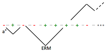
Figure 1: An illustration of the ERM learner as an extreme point of a random walk. Only points to the r.h.s. of $a^{*}$ are depicted. Positive points are correctly labeled; the labels of negative points are due to noise.

Now we will analyze the “deviation” random variable $D:=|\hat{a}-a^{*}|$. (In case of non-unique $\hat{a}$, define $D$ to be the “worst” deviation.) Let $D_{+}$ be the distance from $a^{*}$ to the farthest empirical optimum to its right and define $D_{-}$ analogously on the left. Clearly, $D_{+},D_{-}$ are independent and identically distributed, and $D=\max(D_{+},D_{-})$. Hence

$$\mathbb{E}[D]\leq 2\mathbb{E}[D_{+}].$$

We will define the random variable $T$ as the last time that the drunkard visits the bottommost point (i.e., minimum) of his entire walk. Note that $T$ and $D_{+}$ have the same distribution. Now, as $n\rightarrow\infty$, we use Theorem 1 and substitute $4pq=4\eta-4\eta^{2}$, and we get that with probability $1-\delta$, the ERM algorithm will produce a hypothesis $\hat{a}$ such that

$$|a^{*}-\hat{a}| \;\in\; O\left(\frac{\log{{({1}/{\delta})}}}{\log{({1}/{(\eta-\eta^{2})})}}\right)\;\subset\;O\left(\frac{\log{(1/\delta)}}{(1-2\eta)^{2}}\right).$$

Finally, we can get rid of our assumption that the data lies on arbitrarily many integer points on the line by making the following two observations:

1. Our argument does not require the sample to be on integer points. Rather, the “drunkard” takes a step upon encountering a new point, so as long as he sees

   $$m=O\left(\frac{\log{{(1/\delta)}}}{\log(1/(\eta-\eta^{2}))}\right)$$

   data points within $\varepsilon$ from $a^{*}$, the ERM hypothesis will also be within distance $\varepsilon$.

2. Given that the algorithm has seen sufficiently many points (denoted $m$ above) within $\varepsilon$ of $a^{*}$, seeing additional data is not necessary for the algorithm to succeed (in fact, it only increases the probability of failure). Hence, seeing only $m$ samples is sufficient.

This completes the proof. ∎

To analyze the case of an interval, we must again compare the ERM hypothesis with the true interval. The size overlap between the ERM and the target will guide how many points need to be within $\epsilon$ of both thresholds. As before, focus on analyzing an idealized problem, where the interval simply contains points from a set. Theorem 6 gives a bound on the number of points needed.

Corollary 13 (To Theorem 6).

Let $h_{(a^{*},b^{*})}$ be the target interval. There exists an $m_{0}=m_{0}(\delta,\eta)$, of magnitude

$$m_{0}=\tilde{O}\left(\frac{\log{{({1}/{\delta})}}}{\log{({1}/{(\eta-\eta^{2})})}}\right)\subset\tilde{O}\left(\frac{\log{{(1/\delta)}}}{(1-2\eta)^{2}}\right),$$

such that if the sample contains $m\geq m_{0}$ data points both in the intervals $[a^{*}-\varepsilon,a^{*})$, $(a^{*},a^{*}+\varepsilon]$, $[b^{*}-\varepsilon,b^{*})$, and $(b^{*},b^{*}+\varepsilon]$ then any ERM learner will output a hypothesis $h_{(\hat{a},\hat{b})}$ such that both $|a^{*}-\hat{a}|\leq\varepsilon$ and $|b^{*}-\hat{b}|\leq\varepsilon$ hold with probability at least $1-\delta$.

Proof.

We follow the logic of the proof of Theorem 12, but using the bound from Theorem 6 instead of Theorem 1. We again substitute $4pq=4\eta-4\eta^{2}$ (as $q=\eta$ and $p=1-\eta$), which cancels the $(p-q)^{4}=1$. The remaining difference, the term of $n$, only a polylog factor to the analysis of the sample complexity. ∎

4.3 Relationship to PAC learning

Let us briefly recall the (proper) noisy PAC learning model (Angluin and Laird, 1987; Kearns and Vazirani, 1997). A teacher and a learner agree on the instance space $\mathcal{X}$ and concept class $\mathcal{C}\subset\left\{0,1\right\}^{\mathcal{X}}$. The teacher privately chooses any $c\in\mathcal{C}$ and any distribution $D$ over $\mathcal{X}$. He proceeds to draw $m$ examples i.i.d. $\sim D$ and label each example $x_{i}$ with $c(x_{i})$. Each label is then flipped independently with probability $\eta<1/2$, and the learner gets to see the $m$ examples along with their (potentially corrupted) labels. Based on this noisy sample, the learner produces a hypothesis $h\in\mathcal{C}$, with its associated generalization error

$$\operatorname{err}(h):=\mathbb{P}_{X\sim D}[h(X)\neq c(X)].$$

The learner is $(\varepsilon,\delta)$-successful if

$$\mathbb{P}(\operatorname{err}(h)>\varepsilon)<\delta.$$

A PAC learner is one who is $(\varepsilon,\delta)$-successful whenever $m>m_{0}$, where $m_{0}$ depends on $\mathcal{C},\varepsilon,\delta$ but, crucially, not $c$ or $D$.

We will now show that the adversarial design result we proved for thresholds in Theorem 12 has implications for noisy PAC learnability of this concept class under the uniform distribution. Formally, we take $\mathcal{X}=[0,1]$ with uniform distribution and $\mathcal{C}$ to be the collection of thresholds $c_{a}$, as defined above.

Corollary 14.

Thresholds are (properly) PAC learnable, with label noise $0\leq\eta<1/2$, under the uniform distribution over $[0,1]$, by any ERM algorithm that has access $m\geq m_{0}$ i.i.d. examples, for

$$m_{0}=O\left(\frac{\log^{2}{(1/\delta)}}{\varepsilon(1-2\eta)^{2}}\right).$$

Proof.

Theorem 12 says that we require $m=\Omega\left(\frac{\log{(1/\delta)}}{(1-2\eta)^{2}}\right)$ data points within $\varepsilon$ to the left and right of the target, $a^{*}$. This will happen after $O(\log(1/\delta)m/\varepsilon)$ points are drawn from the uniform distribution, giving a sample complexity of $O\left(\frac{\log^{2}{(1/\delta)}}{\varepsilon(1-2\eta)^{2}}\right)$ and showing the PAC learnability of thresholds under the uniform distribution with an ERM algorithm. Note that in the event that the target threshold $a^{*}$ lies within $\varepsilon$ of a boundary ($0$ or $1$), we only need points to one side of the threshold, and the same analysis goes through. ∎

4.4 Discussion

While our random walk techniques gave a nice illustration of their usefulness via an application to learning, it is possible to get these learning guarantees more simply. To obtain our asymptotic learning results in Theorem 12 and Corollary 14, to get learnability results for thresholds and intervals, we only cared about the order of the points, not the underlying distribution. Hence, these results can alternatively be obtained by reducing toPAC learning under the uniform distribution over the unit interval. Combining results for random classifciation noise (or the noise condition of Massart et al. (2006)) with VC bounds, we can cocnlude that

$$\mathbb{P}(h_{\hat{a}}(x)\neq h_{a*}(x))\leq O\left(\frac{\log 1/\delta}{m(1-2\eta)^{2}}\right),$$

which is sufficient for the purposes of these theorems. This analysis, however is not general and leads us to the following open problem.

Open problem: A natural high-dimensional analogue of thresholds are half-spaces:

$$\mathcal{H}=\left\{\boldsymbol{\mathrm{x}}\mapsto\operatorname{sign}(\boldsymbol{\mathrm{w}}\cdot\boldsymbol{\mathrm{x}}):\boldsymbol{\mathrm{w}}\in\mathbb{R}^{d}\right\}.$$

For some $p\geq 1$, define the loss

$$\ell_{p}(\boldsymbol{\mathrm{w}},\boldsymbol{\mathrm{w}}^{\prime}) = \left\|\boldsymbol{\mathrm{w}}-\boldsymbol{\mathrm{w}}^{\prime}\right\|_{p}=\left(\sum_{i=1}^{d}|w_{i}-w_{i}^{\prime}|^{p}\right)^{1/p}.$$

The noise process is the same as for the thresholds: each label is flipped with probability $0\leq\eta<1/2$. What non-trivial property must the training data satisfy in order to assure learnability under adversarial design? One possibly helpful fact is that a half-space also imposes an “ordering" (similar to the ordering implicitly used by our threshold analysis) on the points along the normal to its hyperplane, and that $n$ points in $d$ dimensions only admit $O(n^{d})$ different orderings when projected onto lines (Cover, 1967).

References

- Agarwal and Duchi [2013] Alekh Agarwal and John C. Duchi. The generalization ability of online algorithms for dependent data. IEEE Trans. Inf. Theory, 59(1):573–587, 2013.
- Anava et al. [2013] Oren Anava, Elad Hazan, Shie Mannor, and Ohad Shamir. Online learning for time series prediction. In Shai Shalev-Shwartz and Ingo Steinwart, editors, COLT 2013 - The 26th Annual Conference on Learning Theory, June 12-14, 2013, Princeton University, NJ, USA, volume 30 of JMLR Workshop and Conference Proceedings, pages 172–184. JMLR.org, 2013.
- Angluin and Laird [1987] Dana Angluin and Philip D. Laird. Learning from noisy examples. Machine Learning, 2(4):343–370, 1987.
- Audiffren and Ralaivola [2015] Julien Audiffren and Liva Ralaivola. Cornering stationary and restless mixing bandits with remix-ucb. In Corinna Cortes, Neil D. Lawrence, Daniel D. Lee, Masashi Sugiyama, and Roman Garnett, editors, Advances in Neural Information Processing Systems 28: Annual Conference on Neural Information Processing Systems 2015, December 7-12, 2015, Montreal, Quebec, Canada, pages 3339–3347, 2015.
- Bateman [1981] Harry Bateman. Higher Transcendental Functions. Krieger Pub Co, 1981. ISBN 0898742064.
- Cesa-Bianchi and Lugosi [2006] Nicolò Cesa-Bianchi and Gábor Lugosi. Prediction, learning, and games. Cambridge University Press, Cambridge, 2006.
- Cover [1967] Thomas M Cover. The number of linearly inducible orderings of points in d-space. SIAM Journal on Applied Mathematics, 15(2):434–439, 1967.
- Gamarnik [2003] David Gamarnik. Extension of the PAC framework to finite and countable Markov chains. IEEE Trans. Inform. Theory, 49(1):338–345, 2003.
- Gofer [2014] Eyal Gofer. Machine Learning Algorithms with Applications in Finance. PhD thesis, Tel Aviv University, 2014.
- Gradshteyn and Ryzhik [2007] I. S. Gradshteyn and I. M. Ryzhik. Table of integrals, series, and products. Elsevier/Academic Press, Amsterdam, seventh edition, 2007. ISBN 978-0-12-373637-6; 0-12-373637-4. Translated from the Russian, Translation edited and with a preface by Alan Jeffrey and Daniel Zwillinger, With one CD-ROM (Windows, Macintosh and UNIX).
- Harik et al. [1999] George Harik, Erick Cantú-Paz, David E Goldberg, and Brad L Miller. The gambler’s ruin problem, genetic algorithms, and the sizing of populations. Evolutionary Computation, 7(3):231–253, 1999.
- Herbrich and Williamson [2002] Ralf Herbrich and Robert C. Williamson. Algorithmic luckiness. Journal of Machine Learning Research, 3:175–212, 2002.
- Karandikar and Vidyasagar [2002] Rajeeva L. Karandikar and Mathukumalli Vidyasagar. Rates of uniform convergence of empirical means with mixing processes. Statist. Probab. Lett., 58(3):297–307, 2002. ISSN 0167-7152.
- Kearns [1998] Michael J. Kearns. Efficient noise-tolerant learning from statistical queries. J. ACM, 45(6):983–1006, 1998.
- Kearns and Schapire [1994] Michael J. Kearns and Robert E. Schapire. Efficient distribution-free learning of probabilistic concepts. J. Comput. Syst. Sci., 48(3):464–497, 1994. ISSN 0022-0000.
- Kearns et al. [1994] Michael J. Kearns, Robert E. Schapire, and Linda Sellie. Toward efficient agnostic learning. Machine Learning, 17(2-3):115–141, 1994.
- Kearns and Vazirani [1997] Micheal Kearns and Umesh Vazirani. An Introduction to Computational Learning Theory. The MIT Press, 1997.
- Koolen and Vovk [2014] Wouter M. Koolen and Vladimir Vovk. Buy low, sell high. Theoretical Computer Science, 558:144 – 158, 2014. ISSN 0304-3975. doi: https://doi.org/10.1016/j.tcs.2014.09.030. URL http://www.sciencedirect.com/science/article/pii/S0304397514007087. Algorithmic Learning Theory.
- Koshy [2009] Thomas Koshy. Catalan numbers with applications. Oxford University Press, Oxford, 2009. ISBN 978-0-19-533454-8.
- Kuznetsov and Mohri [2015] Vitaly Kuznetsov and Mehryar Mohri. Learning theory and algorithms for forecasting non-stationary time series. In Corinna Cortes, Neil D. Lawrence, Daniel D. Lee, Masashi Sugiyama, and Roman Garnett, editors, Advances in Neural Information Processing Systems 28: Annual Conference on Neural Information Processing Systems 2015, December 7-12, 2015, Montreal, Quebec, Canada, pages 541–549, 2015.
- Levin et al. [2017] David A. Levin, Yuval Peres, and Elizabeth L. Wilmer. Markov chains and mixing times. American Mathematical Society, Providence, RI, 2017. ISBN 978-1-4704-2962-1. Second edition of [ MR2466937], With a chapter on “Coupling from the past” by James G. Propp and David B. Wilson.
- London et al. [2012] Ben London, Bert Huang, and Lise Getoor. Improved generalization bounds for large-scale structured prediction. In NIPS Workshop on Algorithmic and Statistical Approaches for Large Social Networks, 2012.
- London et al. [2013] Ben London, Bert Huang, Benjamin Taskar, and Lise Getoor. Collective stability in structured prediction: Generalization from one example. In Proceedings of the 30th International Conference on Machine Learning (ICML-13), 2013.
- Massart et al. [2006] Pascal Massart, Élodie Nédélec, et al. Risk bounds for statistical learning. The Annals of Statistics, 34(5):2326–2366, 2006.
- Mohri and Rostamizadeh [2008] Mehryar Mohri and Afshin Rostamizadeh. Rademacher complexity bounds for non-i.i.d. processes. In Neural Information Processing Systems (NIPS), 2008.
- Mohri and Rostamizadeh [2010] Mehryar Mohri and Afshin Rostamizadeh. Stability bounds for stationary phi-mixing and beta-mixing processes. Journal of Machine Learning Research, 11:789–814, 2010.
- Rostamizadeh and Mohri [2007] Afshin Rostamizadeh and Mehryar Mohri. Stability bounds for non-i.i.d. processes. In Neural Information Processing Systems (NIPS), 2007.
- Rudelson and Vershynin [2009] Mark Rudelson and Roman Vershynin. Smallest singular value of a random rectangular matrix. Commun. Pure Appl. Math., 62(12):1707–1739, 2009.
- Shalizi and Kontorovich [2013] Cosma Rohilla Shalizi and Aryeh Kontorovich. Predictive PAC learning and process decompositions. In Neural Information Processing Systems (NIPS), 2013.
- Shawe-Taylor et al. [1998] John Shawe-Taylor, Peter L. Bartlett, Robert C. Williamson, and Martin Anthony. Structural risk minimization over data-dependent hierarchies. IEEE Transactions on Information Theory, 44(5):1926–1940, 1998.
- Steinwart and Christmann [2009] Ingo Steinwart and Andreas Christmann. Fast learning from non-i.i.d. observations. In NIPS, pages 1768–1776, 2009.
- Steinwart et al. [2009] Ingo Steinwart, Don Hush, and Clint Scovel. Learning from dependent observations. Journal of Multivariate Analysis, 100(1):175 – 194, 2009.
- Teichmann [2015] Josef Teichmann. Foundations of martingale theory and stochastic calculus from a finance perspective, 2015.
- Toth [2001] Balint Toth. No more than three favorite sites for simple random walk. The Annals of Probability, 29(1):484–503, 2001.
- Tsybakov [2004] Alexandre B. Tsybakov. Introduction à l’estimation non-paramétrique, volume 41 of Mathématiques & Applications (Berlin) [Mathematics & Applications]. Springer-Verlag, Berlin, 2004. ISBN 3-540-40592-5.
- Valiant [1984] Leslie G. Valiant. A theory of the learnable. Commun. ACM, 27(11):1134–1142, 1984.
- Zimin and Lampert [2017] Alexander Zimin and Christoph H. Lampert. Learning theory for conditional risk minimization. In Aarti Singh and Xiaojin (Jerry) Zhu, editors, Proceedings of the 20th International Conference on Artificial Intelligence and Statistics, AISTATS 2017, 20-22 April 2017, Fort Lauderdale, FL, USA, volume 54 of Proceedings of Machine Learning Research, pages 213–222. PMLR, 2017.
- Zou et al. [2014] Bin Zou, Zong-ben Xu, and Jie Xu. Generalization bounds of ERM algorithm with Markov chain samples. Acta Mathematicae Applicatae Sinica (English Series), pages 1–16, 2014.