ALMA observations of NGC 6334S $-$ I:
Forming massive stars and cluster in subsonic and transonic filamentary clouds

Abstract

We present Atacama Large Millimeter/submillimeter Array (ALMA) and Karl G. Jansky Very Large Array (JVLA) observations of the massive infrared dark cloud NGC 6334S (also known as IRDC G350.56+0.44), located at the southwestern end of the NGC 6334 molecular cloud complex. The H¹³CO⁺ and the NH₂D lines covered by the ALMA observations at a $\sim$3^′′ angular resolution ($\sim$0.02 pc) reveal that the spatially unresolved non-thermal motions are predominantly subsonic and transonic, a condition analogous to that found in low-mass star-forming molecular clouds. The observed supersonic non-thermal velocity dispersions in massive star forming regions, often reported in the literature, might be significantly biased by poor spatial resolutions that broaden the observed line widths due to unresolved motions within the telescope beam. Our 3 mm continuum image resolves 49 dense cores, whose masses range from 0.17 to 14 $M_{\odot}$. The majority of them are resolved with multiple velocity components. Our analyses of these gas velocity components find an anti-correlation between the gas mass and the virial parameter. This implies that the more massive structures tend to be more gravitationally unstable. Finally, we find that the external pressure in the NGC 6334S cloud is important in confining these dense structures, and may play a role in the formation of dense cores, and subsequently, the embedded young stars.

1 Introduction

Molecular clouds in the Milky Way are in general inefficient in forming stars ($\sim$1%, Myers et al., 1986; Murray, 2011; Vutisalchavakul et al., 2016), an observation that has motivated the long-standing hypotheses that they are supported by supersonic turbulence or magnetic fields against their self-gravitational collapse (for the review see Vazquez-Semadeni et al., 2000; Mac Low & Klessen, 2004; Bergin & Tafalla, 2007; McKee & Ostriker, 2007). Larson (1981) reported an empirical, positive correlation between the physical size scale and the velocity dispersion of molecular clouds. Although the study was based on measurements from different clouds, this correlation has been taken as indications that turbulence dissipates toward smaller spatial scales where gas is prone to the gravitational collapse and the subsequent star-formation (see Bonazzola et al., 1987; Stone et al., 1998; Mac Low et al., 1998; Mac Low & Klessen, 2004; Krumholz & McKee, 2005; Elmegreen & Scalo, 2004; Hennebelle & Chabrier, 2008, and references therein). As a consequence, on spatial scales of dense star-forming cores ($\lesssim$0.1 pc), the non-thermal motions may be sonic (Myers & Goodman, 1988; Goodman et al., 1998; Caselli et al., 2002). This is consistent with the observations of some filamentary, low-mass star-forming clouds (e.g., Hacar & Tafalla, 2011; Hacar et al., 2013; Pineda et al., 2015; Hacar et al., 2016b, 2017).

In contrast, previous observations towards high-mass star-forming regions have reported supersonic non-thermal velocity dispersion (Caselli & Myers, 1995; Pirogov et al., 2003; Shirley et al., 2003; Wang et al., 2008; Vasyunina et al., 2011; Sanhueza et al., 2012; Li et al., 2017). The formation of gas cores of high mass and high density may be supported by supersonic turbulence. Otherwise they may fragment to form lower-mass stars since their masses are much larger than the Jeans mass (McKee & Tan, 2003). However, recent higher angular resolution observations started to reveal subsonic non-thermal velocity dispersion in massive star-forming molecular clouds on small spatial scales (e.g., Beuther et al., 2018; Hacar et al., 2018; Monsch et al., 2018; Sokolov et al., 2018). Whether the massive star- and cluster-forming regions are initially supported by supersonic turbulence remains a matter of debate, and needs to be clarified with more observations of target sources at early evolutionary stages.

Using the Atacama Large Millimeter Array (ALMA) and the Karl G. Jansky Very Large Array (JVLA), we have carried out high angular resolution observations towards the infrared dark, massive cluster-forming molecular cloud NGC 6334S, which is located at the southwestern end of the NGC 6334 molecular cloud complex. In contrast to the other luminous OB cluster-forming clumps in the NGC 6334 molecular cloud complex, namely the I, I(N), II, III, IV, and V clumps (Persi & Tapia, 2008; Russeil et al., 2013; Willis et al., 2013), NGC 6334S is dark at IR wavelengths and lacks signs of massive star formation (see Figure 1). With a mass of 1.3 $\times$ 10³ $M_{\odot}$, comparable to the clumps with embedded massive protostars and protocluster in the complex, NGC 6334S has the potential to form massive stars with a cluster of lower mass objects. The proximity of NGC 6334S ($d\sim$1.3 kpc; Chibueze et al., 2014) makes it an ideal laboratory to investigate the key physical processes related to massive star and cluster formation.

In this paper, we investigate the dynamical motions of identified embedded dense cores and their parent cloud, as well as the dynamical stability of dense cores. First, we describe our ALMA and JVLA observations in $\S$ 2. Then, we present the results and analysis in $\S$ 3. We discuss in detail the properties of dense cores and their parent cloud in $\S$ 4. Finally, we summarize the conclusion of this work in $\S$ 5.

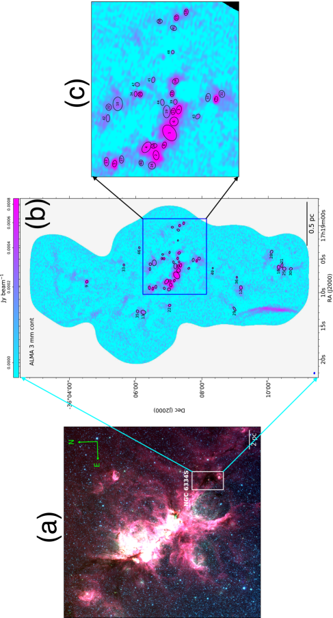
Figure 1: Panel a: three-color Spitzer composite image of the NGC 6334 molecular cloud complex with blue, green, and red representing data at $\lambda$ = 3.6, 4.5, and 8.0 $\mu\rm m$, respectively. The image is centered at 17h20m02s, -35d54m03s. The scale bar is approximately 2 pc at the distance of 1.3 kpc. The white box presents the NGC 6334S region. Panel b: the ALMA 3 mm continuum image. The beam size is shown in the bottom left of the panel. Panel c: zoom in of the central region. The black ellipses present the identified dense cores.

2 Observations

2.1 ALMA Observations

We carried out a 55-pointings mosaic of the massive infrared dark cloud (IRDC), NGC 6334S, between 2017 March 13 and 2017 March 21 using the 12-m main array of ALMA (ID: 2016.1.00951.S, PI: Shaye Strom). The overall observing time and the on-source integration time are 7.3 hours and 4.4 hours, respectively. The projected baseline lengths range from 15 to 155 meters ($\sim$4.9-51 k$\lambda$ at the averaged frequency of 98.5 GHz).

We employed two 234.4 MHz wide spectral windows to cover the H¹³CO⁺ 1-0 (86.754 GHz) and NH₂D $1_{11}$-$1_{01}$ (85.926 GHz) lines, respectively, with a spectral resolution of 61 kHz ($\sim$0.21 km s^-1 at 86 GHz). In addition, we centered three 1.875 GHz wide spectral windows at 88.5 GHz, 98.5 GHz, and 100.3 GHz to obtain broad band continuum data. We observed the quasars J1617-5858, J1713-3418, and J1733-1304, for passband, complex gain, and absolute flux calibrations, respectively.

The data calibrations were performed by the supporting staff at the ALMA Regional Center (ARC), using the CASA software package (McMullin et al., 2007). The continuum image was obtained using the three 1.875 GHz spectral windows with a Briggs’s robust weighting of 0.5 to the visibilities. This yields a synthesized beam of 3^′′.6 $\times$ 2^′′.4 (or 0.023 $\times$ 0.015 pc) with a position angle (P.A.) of 81^∘ and a 1$\sigma$ root mean square (rms) noise level of 0.03 mJy beam^-1. For both H¹³CO⁺ and NH₂D lines, we used a Briggs’s robust weighting of 0.5 to the visibilities, which achieved a synthesized beam of about 4^′′.1 $\times$ 2^′′.8 (PA= 83^∘, or 0.026 $\times$ 0.018 pc) for these two lines. The 1$\sigma$ rms noise level is about 6 mJy beam^-1 per 0.21 km s^-1 channel for both the H¹³CO⁺ and NH₂D lines.

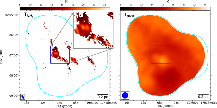
Figure 2: Left: temperatures derived from the NH₃ data. The cyan line is the JVLA mosaic pattern. Right: the dust temperatures derived from SED fitting. The blue box marks the zooming in region in the left panel. The beam size is shown in the bottom left of the panel.

2.2 JVLA Observations

We carried out a 4-pointings mosaic of the central region of NGC 6334S using the JVLA, on 2014 August 28 (project code: 14A-241; PI: Qizhou Zhang). These observations simultaneously covered the NH₃ (1,1) through (5,5) metastable inversion transitions. The overall observing time was 2 hours, which yielded an on-source integration of $\sim$20 minutes for each pointing. The Quasars 3C286, J1743-0350 and J1744-3316 were observed for flux, bandpass and gain calibrations, respectively.

The data calibration and imaging were carried out using the CASA software package. Our target source is located in the south, which leads to shorter projected baselines in the north-south direction. To increase the signal-to-noise (S/N) ratio, we tapered the visibilities with an elliptical Gaussian with full width at half-maximum (FWHM) of 6^′′$\times$ 3^′′ (P.A. = 0^∘). The achieved synthesized beam size is about 10^′′$\times$ 5^′′ (P.A. = 26^∘, or 0.063 $\times$ 0.032 pc) for the NH₃ (1,1) and (2,2) lines. The continuum image achieved a 1$\sigma$ rms noise of 30 $\mu$Jy beam^-1, while spectral line images achieved a 1$\sigma$ rms noise of 9 mJy beam^-1 at a spectral resolution of 0.2 km s^-1.

2.3 Fitting molecular line spectra

We fit Gaussian line profiles to the H¹³CO⁺ image cube pixel by pixel, using the PySpecKit package (Ginsburg & Mirocha, 2011). We excluded regions where the peak intensity in the spectral domain is below 5 times the rms noise level. For data above the cutoff, we regarded spectral peaks that are separated by more than 2 spectral channels and brighter than 5 times the rms noise level as independent velocity components. We then simultaneously fit Gaussian profiles to all of the independent velocity components. We eliminated poor fits by only keeping pixels that fulfill the following criteria: (1) $\sigma_{\rm obs}$ $>$ 3$\Delta_{\sigma_{\rm obs}}$, which ensures that the derived observed velocity dispersion is reliable. (2) -8 $\leqslant$ $v_{\rm lsr}\leqslant$ 0 km s^-1, which is the H¹³CO⁺ line emission velocity range in the NGC 6334S. (3) $I>$ 3$\Delta_{I}$. (In these criteria, $\Delta_{\sigma_{\rm obs}}$ is the uncertainty of the observed velocity dispersion $\sigma_{\rm obs}$, $v_{\rm lsr}$ is the central velocity, and $\Delta_{I}$ is the uncertainty of velocity integrated intensity $I$.) The observed velocity dispersion, $\sigma_{\rm obs}$, is the combination of both thermal and non-thermal velocity dispersion values. The NH₂D line cubes were fit following a similar routine but including its 36 hyperfine components (Daniel et al., 2016).

The NH₃ (1,1) and (2,2) transitions were jointly fit, pixel by pixel, using PySpecKit in order to estimate the gas kinetic temperature and the line width. Details of the procedure have been provided in Friesen et al. (2017). Limited by S/N ratios, we cannot robustly fit multiple velocity components to the NH₃ spectra. Nevertheless, for our purpose of deriving the gas temperature and assessing the uncertainty of converting the NH₃ rotational temperature to the gas kinetic temperature, it is adequate to assume a single velocity component. We have compared the gas temperatures estimated from NH₃ and dust temperatures estimated by SED fitting the PACS 160 $\mu\rm m$, SPIRE 250 $\mu\rm m$, PLANCK and ATLASGAL 870 $\mu\rm m$  data (see Appendix A). In spite of the different angular resolutions, we found that the derived gas and dust temperatures are consistent to within $\leqslant$ 3 K at the central part of NGC 6334S, and are consistent to around 6 K over a more extended area (Figure 2). We use a uniform temperature of $\langle T_{\rm NH_{3}}\rangle$ = 15 K, the averaged temperature from the NH₃ data, to calculate the gas masses, thermal line widths and the sound speeds for the regions where the NH₃ data are not available (see Section 3.3 and Section 3.4).

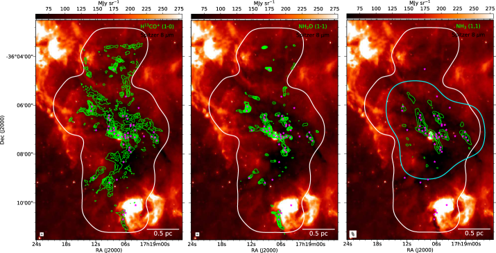
Figure 3: Figure shows the velocity integrated intensity map (green contours) of the H¹³CO⁺ (1-0), NH₂D (1-1), and NH₃ (1,1) overlaid on the Spitzer 8 $\mu\rm m$ emission. The green contours are $\pm$(3, 6, 9 ….) $\times$ $\sigma$, where $\sigma$ is the rms level for each line. The pink stars mark the dense cores revealed in the 3 mm continuum data. The white and cyan solid lines show the ALMA and VLA primary-beam responses at 20%, respectively. The beam size is shown in the bottom right of the panel.

3 Results and Analysis

The present work focuses on the non-thermal velocity dispersion of the NGC 6334S cloud and the embedded dense cores, as well as the stability of the dense cores. Both H¹³CO⁺ 1-0 (critical density, n${}_{\rm cr}\sim$ 2 $\times$10⁴ cm^-3) and NH₂D $1_{11}$-$1_{01}$ (n${}_{\rm cr}\sim$ a few 10⁵ cm^-3) are good dense gas tracers in star formation regions (e.g., Pillai et al., 2007; Busquet et al., 2010; Sanhueza et al., 2012), which allows us to investigate the kinematic properties on spatial scales of both molecular cloud and dense cores. The H¹³CO⁺ molecule ($\mu$ = 30, $\sigma_{\rm th(15\rm K)}$ = 0.06 km s^-1) has a higher molecular weight than the NH₂D molecule ($\mu$ = 18, $\sigma_{\rm th(15\rm K)}$ = 0.08 km s^-1), and therefore is a better probe of the non-thermal gas motions. In spite of the hyperfine line splitting of the H¹³CO⁺ 1-0 transitions with six components, they are closer than 0.14 km s^-1 (41 kHz) at the frequency of the H¹³CO⁺ 1-0 line (Schmid-Burgk et al., 2004). The averaged line width reduction is about 0.01 km s^-1 when the hyperfine structure of the H¹³CO⁺ is fully taken into account, which is much smaller than the derived line widths (Section 3.3). Therefore, the hyperfine components of the H¹³CO⁺ 1-0 can be treated as the same transition for our analysis. The main hyperfine line components of the NH₂D 1-1 line are resolved by the observations, which permits robustly deriving the line widths towards the localized cores with higher gas column densities (e.g., Pillai et al., 2011). When there are multiple velocity components along the line-of-sight, they can be confused with the hyperfine line structures of the NH₂D. Nevertheless, this issue can be mitigated by comparing them with the spectrum of the H¹³CO⁺ line. Finally, the multiple inversion line transitions of NH₃ can be simultaneously covered by the observations of JVLA thanks to its broad bandwidth capability.

3.1 Dense core identification

We employed the astrodendro algorithm to pre-select dense cores (i.e., the leaves in the terminology of astrodendro) from the 3 mm continuum image (Figure 1). The specific properties of the dense cores (size, flux density, peak intensity and position) identified from the astrodendro analysis are obtained using the CASA-imfit task. There are some compact sources that are detected at $>$ 5$\sigma$ significance but missed by astrodendro; we use CASA-imfit to recover them from the image. We avoid identifying sources from the elongated filament southeast of NGC 6334S (Figure 1). This elongated filament is not detected with spectral line emission counterpart, and is likely dominated by free-free or synchrotron emission and likely associated with the Hii region east of this filament. When computing the dendrogram the following parameters are used: the minimum pixel value $\mathbf{min_{-}value}$ = 3$\sigma$, where $\sigma$ is the rms noise of continuum image; the minimum difference in the peak intensity between neighboring compact structures $\mathbf{min_{-}delta}$ = 1$\sigma$; the minimum number of pixels required for a structure to be considered an independent entity $\mathbf{min_{-}npix}$ = 40, which is approximately the synthesized beam area.

We identified 49 dense cores (Table 1), which are labelled in Figure 1 and presented as pink stars in Figure 3. They are closely associated with gas filamentary structures, and the majority (39) of these cores are concentrated in the central 1 pc area of the image.

3.2 Intensity distributions of molecular gas tracers

Figure 3 shows the velocity integrated intensity maps of the H¹³CO⁺, NH₂D and NH₃ emission, overlaid with the Spitzer 8 $\mu\rm m$ emission. We detected significant H¹³CO⁺ line emission coinciding with the 8 $\mu\rm m$ dark filamentary structures, as well as with the majority of embedded dense cores. On the other hand, the NH₂D and NH₃ line emissions are preferentially detected at the location of dense cores.

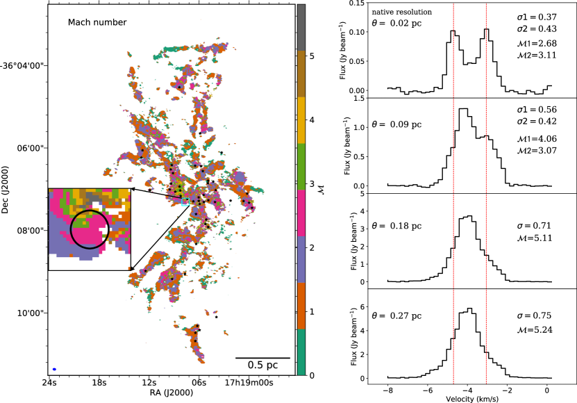
Figure 4: Left: Mach number map estimated from the H¹³CO⁺ line for NGC 6334S. The black stars represent the identified dense cores. The beam size is shown in the bottom left of the panel. Right: averaged spectrum of the H¹³CO⁺ line within the black circle showed on the left panel with different beam sizes. The two dashed vertical lines show the central velocities of the two velocity components measured at the native spatial resolution. The beam sizes ($\theta$), velocity dispersion ($\sigma_{\rm obs}$) and Mach number are presented inside the panel.

3.3 Line width and Mach number

3.3.1 $\rm H^{13}CO^{+}$

Single, double and triple velocity components were resolved in 84.8%, 15.1% and 1.1% of the areas where significant H¹³CO⁺ emission was detected (Table 2). We refer to spectra with single, double and triple velocity components as $v$1, $v$2 and $v$3, respectively. We found a $\langle\sigma_{\rm obs}\rangle$ = 0.31 km s^-1 mean observed velocity dispersion from the dense cores, and a $\langle\sigma_{\rm obs}\rangle$ = 0.23 km s^-1 mean observed velocity dispersion exterior to the dense cores. The area of each dense core is marked with an open ellipse in Figure 1, while the remaining regions in the NGC 6334S are defined as areas exterior to the dense cores. The non-thermal velocity dispersion ($\sigma_{\rm nt}$) of the H¹³CO⁺ line was estimated by $\sigma_{\rm nt}=\sqrt{\left(\sigma_{\rm obs}^{2}-\triangle_{\rm ch}^{2}/(2\sqrt{2\;\rm ln\;2})^{2}\right)-\sigma_{\rm th}^{2}}$, where $\triangle_{\rm ch}$ and $\sigma_{\rm th}$ are velocity channel width and thermal velocity dispersion, respectively. The molecular thermal velocity dispersion was estimated by $\sigma_{\rm th}$ = $\sqrt{(k_{\rm B}T)/(\mu\,m_{\rm H})}$ = 9.08 $\times$ 10^-2 km s${}^{-1}\left(\frac{T}{\rm K}\right)^{0.5}\mu^{-0.5}$, where $\mu=m/m_{\rm H}$ is the molecular weight, $m$ is the molecular mass, $m_{\rm H}$ is the proton mass, $k_{\rm B}$ is the Boltzmann constant, and $T$ is the gas temperature. The thermal velocity dispersion (sound speed $c_{\rm s}$) of the particle of mean mass was estimated assuming a mean mass of gas of 2.37$\,m_{\rm H}$ (Kauffmann et al., 2008). The gas temperatures, $T_{\rm NH_{3}}$, derived from the NH₃ line ratios were used to calculate the thermal velocity dispersion (Figure 2, see Section 2.3). We assumed a gas kinetic temperature of $\langle T_{\rm NH_{3}}\rangle$ = 15 K for regions where the NH₃ detection is insufficient for our temperature fittings or without NH₃ observations. For each of the velocity components observed from the entire NGC 6334S region we also derived the Mach number, $\mathcal{M}=\sqrt{3}\sigma_{\rm nt}/c_{\rm s}$. The derived Mach numbers range from 0.02 to 6.3, with a mean value of 1.5.

Figure 4 shows the Mach number map of NGC 6334S. From this map, it appears that non-thermal motions in the majority of the observed regions are subsonic or transonic ($0<\mathcal{M}<2$). The upper left panel of Figure 5 shows a normalized histogram of Mach numbers, which is derived from the regions in which is detected one single velocity component. We found that the $\sigma_{\rm nt}$ values of 29.6%, 46.4%, and 24% of these regions are subsonic ($\mathcal{M}\leqslant 1$), transonic ($1<\mathcal{M}\leqslant 2$), and supersonic ($\mathcal{M}>2$), respectively (for a complete summary see Table 2).

The upper right panel of Figure 5 shows the histograms of Mach numbers derived from all observed velocity components. The contribution from the areas of dense cores and from the areas exterior to the dense cores are distinguished with colors. From areas exterior to the dense cores, we observed a histogram similar to the one presented in the left panel of Figure 5. We found systematically higher yet mostly still subsonic-to-transonic Mach numbers in the areas of dense cores. As can be seen from Figure 4, supersonic motions are mostly found in the central part of NGC 6334S, where there are multiple velocity components around dense cores. In summary, the non-thermal motions in the NGC 6334S cloud and the embedded dense cores are predominantly subsonic and transonic.

3.3.2 $\rm NH_{2}D$

In 89.3% and 10.7% of the regions with NH₂D emission, we resolved single and double velocity components, respectively. The mean $\sigma_{\rm obs}$ of the NH₂D line is 0.21 km s^-1 and 0.16 km s^-1 for the dense cores and the remaining region in NGC 6334S, respectively, which are smaller than those of the H¹³CO⁺ line. Explanations for this discrepancy are discussed further in Section 4.2.2. The Mach numbers estimated from the NH₂D line range from 0.01 to 3.7, with a mean value of 1 (Table 2). The majority of cores (89%) have a mean Mach number of less than 2, and 43% of cores have a mean March number smaller than 1. Figure 5 shows the normalized histogram of Mach numbers estimated from the the NH₂D line, which indicates that Mach numbers are smaller than 2 at the majority of regions, and are between 2 and 3 in 4.9% of the observed regions.

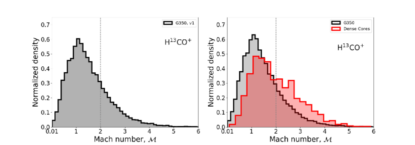
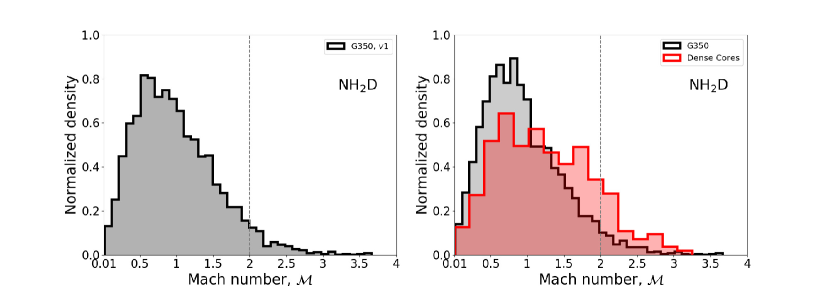
Figure 5: Gaussian kernel density estimate (KDE) of the Mach number distribution. Upper left: the distribution of Mach numbers for regions where a single velocity component was detected in NGC 6334S. Upper right: the distribution of Mach number for all velocity components for the entire NGC 6334S excluding the dense cores (black histogram), and for all velocity components from the dense cores only (red histogram). Bottom: same as the upper panels but using the NH₂D line. The grey vertical dash-dotted line represents the position of Mach number equal to 2.

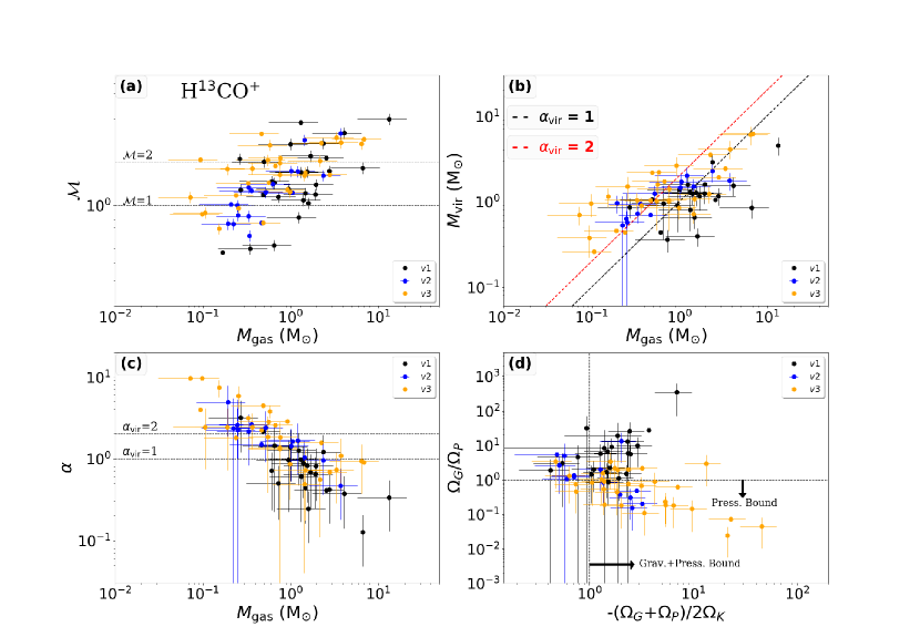
Figure 6: Panel a: Mach number versus gas mass for the H¹³CO⁺ decomposed structures. Panel b: virial mass versus gas mass. The black and red dash-dotted lines show the $\alpha_{\rm vir}$ = 1 and $\alpha_{\rm vir}$ = 2 lines, respectively. Panel c: virial parameter versus gas mass. Panel d: the ratio of $\Omega_{G}$/$\Omega_{P}$ versus ratio of -($\Omega_{G}$ +$\Omega_{P}$)/2$\Omega_{K}$. $v1$, $v2$ and $v3$ represent the single, double and triple velocity components, respectively.

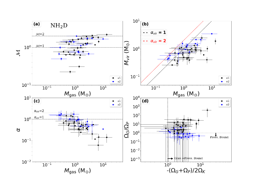
Figure 7: Same as Figure 6 but for the NH₂D decomposed structures.

3.4 Dense Core Properties

With the observed 3 mm continuum fluxes, we estimated the gas mass ($M_{\rm gas}$) of identified cores assuming optically thin modified black body emission in the Rayleigh-Jeans limit, following

$$M_{\rm gas}=\eta\frac{F_{\nu}d^{2}}{B_{\nu}(T)\kappa_{\nu}},$$ (1)

where $\eta$ = 100 is the assumed gas-to-dust mass ratio, $d$ is the source distance, $F_{\nu}$ is the continuum flux at frequency $\nu$, $B_{\nu}(T)$ is the Planck function at temperature $T$, and $\kappa_{\nu}$ is the dust opacity at frequency $\nu$. We adopt $\kappa_{\rm 98.5\;GHz}$ = 0.235 cm²g^-1, assuming $\kappa_{\nu}$ = 10(${\nu}$/1.2 THz)^β cm²g^-1 and $\beta$ = 1.5 for all of dense cores (Hildebrand, 1983).

The derived gas masses are between 0.17 and 14 $M_{\odot}$: two cores have masses of 13 $M_{\odot}$ and 14 $M_{\odot}$; the masses of 12 cores are between 2 and 7 $M_{\odot}$; the masses of the rest of the cores range from 0.17 to 1.97 $M_{\odot}$ (Table 1). Our 1$\sigma$ mass sensitivity corresponds to $\sim$0.03 $M_{\odot}$. The uncertainty in the continuum flux is adopted to be a typical value of 10% in interferometer observations. The uncertainty in distance from the trigonometric parallax measurement is about 20% (Chibueze et al., 2014). The typical uncertainty in temperatures estimated from the NH₃ lines is about 15%, which is mainly due to the low S/N in the NH₃ data. $\eta$ is adopted to be 100 in this study, while its standard deviation is 23 (corresponding to 1$\sigma$ uncertainty of 23%) assuming it is uniformly distributed between 70 and 150 (Devereux & Young, 1990; Vuong et al., 2003; Sanhueza et al., 2017). We adopted a conservative uncertainty of 28% in $\kappa_{\nu}$ (e.g., Sanhueza et al., 2017). Taking into account these uncertainties, we estimate an uncertainty of 57% for the gas mass.

Assuming spherical symmetry for identified dense cores, we evaluated their volume densities ($n_{\rm H_{2}}=M_{\rm gas}/(\mu m_{\rm H}4\pi R^{3}/3)$) using the gas mass and effective radius. The derived volume densities vary between 4.3$\times$10⁵ and 2.2$\times$10⁸ cm^-3, with the mean and median value of 1.1$\times$10⁷ and 2.5 $\times$10⁶ cm^-3, respectively. The typical uncertainty is about 58% for volume density, with the exception of eight marginally resolved cores that have an uncertainty of $>$ 100% due to a large uncertainty in the beam-deconvolved effective radius.

For cores which were resolved with multiple velocity components (Appendix B), we further estimated the gas mass ($M_{i}$) of each individual component $i$ assuming that its continuum flux is $F_{\rm cont}^{i}=F_{\rm cont}^{\rm tot}\times I_{\rm line}^{i}/I_{\rm line}^{\rm tot}$, where $F_{\rm cont}^{\rm tot}$ is the overall continuum flux, $I_{\rm line}^{i}$ is the velocity integrated intensity of the $i$th velocity component, and $I_{\rm line}^{\rm tot}$ = $\sum I_{\rm line}^{i}$ is the overall velocity integrated intensity. This provides a reasonable estimate of gas mass for decomposed structures since the dense cores are dense enough ($>4\times 10^{5}$ cm^-3) for the gas and the dust to be well coupled (Goldsmith, 2001). Using H¹³CO⁺ emission, we have decomposed 67 structures (hereafter decomposed structures).

The virial ratio is evaluated for each decomposed structure using (Bertoldi & McKee, 1992):

$$\alpha_{\rm vir}=\frac{M_{\rm vir}}{M_{\rm gas}}$$ (2)

$$M_{\rm vir}=\frac{5}{a\beta}\frac{\sigma_{\rm tot}^{2}R}{G},$$ (3)

where $M_{\rm vir}$ is the virial mass, $\sigma_{\rm tot}$ = $\sqrt{\sigma_{\rm nt}^{2}+c_{s}^{2}}$ is the total velocity dispersion, $R$ is the effective radius, $G$ is the gravitational constant, parameter $a$ equals to $(1-b/3)/(1-2b/5)$ for a power-law density profile $\rho\propto r^{-b}$ (Bertoldi & McKee, 1992), and $\beta=(\arcsin e)/e$ is the geometry factor. Here, we assume a typical density profile of $b$ = 1.6 for all decomposed structures (Beuther et al., 2002; Butler & Tan, 2012; Palau et al., 2014; Li et al., 2019a). The eccentricity $e$ is determined by the axis ratio of the dense structure, $e=\sqrt{1-f_{\rm int}^{2}}$. The axis ratio of the decomposed structure is assumed to be the value of its corresponding dense core. Considering the projection effect and the dense cores are likely prolate ellipsoids (Myers et al., 1991), the observed axis ratio, $f_{\rm obs}$, is larger than the intrinsic axis ratio, $f_{\rm int}$. The $f_{\rm int}$ can be estimated from $f_{\rm obs}$ with

$$f_{\rm int}=\frac{2}{\pi}\;f_{\rm obs}\;\mathcal{F}_{1}\;(0.5,0.5,-0.5,1.5,1,1-f_{\rm obs}^{2})$$ (4)

(Fall & Frenk, 1983; Li et al., 2013), where $\mathcal{F}_{1}$ is the Appell hypergeometric function of the first kind.

The corresponding virial mass of each velocity component is derived based on the corresponding effective radius, $R_{i}=R\times\sqrt{A_{i}/A_{\rm core}}$. Here, $R_{i}$ is the effective radius for the $i$th velocity component, $R$ is the dense core beam-deconvolved effective radius (Table 1), $A_{i}$ is the number of pixels for the $i$th velocity component within the dense core measured in the moment-zeroth map, and the $A_{\rm core}$ is the number of pixels for the dense core (Figure 8).

Taking into account the uncertainties of $\sigma_{v}$ and $R$, leads to an uncertainty of about 24% for virial mass. With the uncertainties of virial mass and dense core mass, the typical uncertainty is about 46% for the virial ratios, except for three marginal resolved dense cores that have an uncertainty of $>$ 100% due to the large uncertainty in the beam-deconvolved effective radius.

Based on the 67 H¹³CO⁺ decomposed structures, we found that the virial ratios range from 0.1 to 9.7, with the mean and median value of 1.8 and 1.4, respectively. Forty-three out of 67 H¹³CO⁺ decomposed structures have virial ratios smaller than 2, while 27 of them have ratios below 1. Non-magnetized cores with $\alpha_{\rm vir}<$ 2, $\alpha_{\rm vir}\sim$ 1 and $\alpha_{\rm vir}<$ 1 are considered to be gravitationally bound, in hydrostatic equilibrium and gravitationally unstable, respectively (Bertoldi & McKee, 1992; Kauffmann et al., 2013). Those with $\alpha_{\rm vir}>$ 2 could be gravitationally unbound. Figure 6 shows the virial ratio versus the gas mass of the H¹³CO⁺ decomposed structures. From this plot, it is apparent that there is an inverse relationship between the mass and the virial ratio. This indicates that the most massive structures tend to be more gravitationally unstable, while the less massive structures are gravitationally unbound and may eventually be disperse, unless there are other mechanism(s) that help to confine them such as external pressure and/or embedded protostar(s) with a significant mass.

We have decomposed 45 structures with the NH₂D emission. For these NH₂D decomposed structures, the derived virial ratios are between 0.1 and 12, with the mean and median values of 1.3 and 0.6, respectively. All of the NH₂D decomposed structures have virial ratios lower than 2, and 36 of them have ratios smaller than 1. This suggests that these decomposed structures are gravitationally bound. The analysis of both NH₂D and H¹³CO⁺ give a similar result: the virial ratios of the decomposed structures decrease with increasing gas masses.

3.5 Pressure

Previous studies of star-forming regions have suggested that the external pressure provided by the ambient molecular cloud materials might help to confine dense structures in molecular clouds (Kirk et al., 2006; Liu et al., 2013a; Kirk et al., 2017; Seo et al., 2015; Pattle et al., 2015). In order to examine whether the external pressure can play a significant role in confining the dense structures, we estimate the external pressure from the ambient cloud for each decomposed structure (McKee, 1989; Kirk et al., 2017) using:

$$P_{\rm cl}=\pi G\bar{\Sigma}\Sigma_{r}\beta_{\rm cl},$$ (5)

where $P_{\rm cl}$ is the gas pressure, $\bar{\Sigma}$ is the mean column density of the cloud, $\Sigma_{r}$ is the column density integrated from the cloud surface to depth $r$, and $\beta_{\rm cl}$ is the geometry factor for the cloud. We assumed that $\Sigma_{r}$ is equal to half of the observed column density at the footprint of dense structures, $\Sigma_{r}=\Sigma_{\rm obs}$/2, which is reasonable for most of star-forming regions (e.g., Kirk et al., 2006, 2017). To estimate the mean column density of a cloud, we consider only the central region where the mean column density of the cloud is about $\bar{\Sigma}$ = 0.15 g cm^-2 estimated from the SED fitting (see Appendix A).

The derived external pressure of the H¹³CO⁺ decomposed structures is between 9.1$\times 10^{6}$ and 1.9 $\times 10^{8}\,\rm K\,cm^{-3}$, with a mean value of $\langle P_{\rm cl}/k_{\rm B}\rangle=3.8\times 10^{7}\,\rm K\,cm^{-3}$. For the NH₂D decomposed structures, the derived external pressures range from 9.1$\times 10^{6}$ to 1.9$\times 10^{8}\,\rm K\,cm^{-3}$, with a mean value of $\langle P_{\rm cl}/k_{\rm B}\rangle=3.9\times 10^{7}\,\rm K\,cm^{-3}$.

To determine the energy balance, we evaluated the external pressure energy, gravitational potential energy and internal kinetic energy in the virial equation (McKee, 1989; Bertoldi & McKee, 1992):

$$\Omega_{P}=-4\pi P_{\rm cl}R^{3}$$ (6)

$$\Omega_{G}=-\frac{3}{5}a\beta\frac{GM^{2}}{R}$$ (7)

$$\Omega_{K}=\frac{3}{2}M\sigma_{\rm tot}^{2}$$ (8)

where $\Omega_{P}$, $\Omega_{G}$ and $\Omega_{K}$ are the external pressure, gravitational and kinetic terms, respectively.

For the H¹³CO⁺ decomposed structure, the derived $\Omega_{P}$ ranges from 4.8$\times$10⁴⁰ to 4.1$\times$10⁴⁴ erg, the $\Omega_{G}$ is between 3.7$\times$10⁴⁰ and 7.0$\times$10⁴⁴ erg, and the $\Omega_{K}$ is between 3.7$\times$10⁴⁰ and 1.3$\times$10⁴⁴ erg. The NH₂D decomposed structures have similar values compared to that of the H¹³CO⁺ with the $\Omega_{P}$ ranging from 1.5$\times$10⁴¹ to 4.1$\times$10⁴⁴ erg, the $\Omega_{G}$ between 5.9$\times$10⁴¹ and 7.9$\times$10⁴⁴ erg, and the $\Omega_{K}$ between 5.2$\times$10⁴¹ and 5.6$\times$10⁴³ erg.

4 Discussion

4.1 sonic-to-transonic motion

The mean observed values for $\sigma_{\rm obs}$ are about 0.23 km s^-1 (or 0.54 km s^-1 in FWHM) and 0.17 km s^-1 (or 0.40 km s^-1 in FWHM) for H¹³CO⁺ and NH₂D, respectively, which indicates that the observed spectra are resolved in these ALMA observations with a spectral velocity channel width of 0.21 km s^-1 (see also the Appendix C). These line widths may be regarded as conservative upper limits, given the limited spectral resolution, the hyperfine line splittings, the blending of velocity components along the line-of-sight, and the outflows and shocks all of which can lead to overestimates of the line widths (Li et al., 2019b).

In spite of the aforementioned biases, from Figure 5 we can see that the spatially unresolved non-thermal motions are predominantly subsonic and transonic ($\sim$77% regions). The normalized distribution function of $\mathcal{M}$ derived from the H¹³CO⁺ observations peaks at 1.2. We have run a test with temperatures ranging from 8 to 25 K, corresponding to the range of the dust temperatures in the region, and found that 56% to up to 99% of Mach numbers are smaller than 2. This confirms that the Mach numbers are still dominated by subsonic and transonic motions within this temperature range.

More interestingly, such features persist down to the dense core scales ($\sim$0.015 pc) but with a higher fraction of larger Mach numbers as shown in Figure 5. There are several reasons that may cause the relatively broad line widths toward the dense cores. First, the line widths may be broadened by protostellar activities (e.g., outflow, infall, and/or rotation). Second, given that the majority of dense cores are associated with multiple velocity components, the line widths could be enhanced by the intersection of gas components at different velocities. Third, high optical depths could broaden the detected line widths (Hacar et al., 2016a). Unfortunately, we can not discriminate between these possibilities with the data at hand.

The subsonic-to-transonic dominated nature in both dense cores and NGC 6334S cloud suggests that these cores are still at very early evolutionary stages such that the protostellar feedback-induced turbulence is small as compared to the initial turbulence. Such low turbulence is similar to what is seen in low-mass star formation regions, e.g., Musca, L1517, NGC1333 and Taurus (Hacar & Tafalla, 2011; Hacar et al., 2013, 2016b, 2017)

Figure 4 shows the spectral lines of the H¹³CO⁺ at different spatial resolutions. It is clear that the line widths increase with increasing beam sizes. Therefore, the observed supersonic non-thermal velocity dispersions in massive star forming regions often reported in the literature might be significantly biased by the poor spatial resolution, since the spatially unresolved motions within the telescope beam can broaden the observed line widths.

4.2 Dynamical State of Dense Cores

The relationship of decreasing $\alpha_{\rm vir}$ with $M_{\rm gas}$ shown in Figures 6 and 7 has also been reported in previous studies of parsec scale massive clumps (Urquhart et al., 2015; Kauffmann et al., 2013), subparsec scale ($\leqslant 0.1$ pc) massive dense cores (Li et al., 2019a), and low-mass star formation regions (Lada et al., 2008; Foster et al., 2009). Traficante et al. (2018) pointed out that such a decreasing trend of $\alpha_{\rm vir}$ may be attributed to systematic measurement errors when a particular molecular line preferentially traces molecular gas with densities above the critical density of the line transition. This effect could lead to a lower estimate of the virial parameter due to an underestimation of the observed line width. However, this effect may not be significant since the critical density of a given gas tracer is typically higher than the effective excitation density because of the effect of radiative trapping (Shirley, 2015; Hull & Zhang, 2019). The assumption of a certain density profile (equation 3, with $b=1.6$) could introduce some uncertainties to the virial mass, while it does not appear to be the dominant factor in the inverse $\alpha_{\rm vir}-M_{\rm gas}$ relation since the density structures do not show significant differences between the massive cores and the low-mass cores (see for example, van der Tak et al., 2000; Motte & André, 2001; Mueller et al., 2002; Shirley et al., 2002; Beuther et al., 2002; Butler & Tan, 2012; Palau et al., 2014; Tobin et al., 2015; Li et al., 2019a).

Chemical segregation may introduce biases in the measurements of $M_{\rm vir}$. For example, the study of the B-type star-forming region G192.16-3.84 (Liu et al., 2013b) found that the H¹³CO⁺ emission did not trace the gravitationally accelerated, high-velocity gas that is probed by the H¹³CN emission and other hot core tracers. The decreasing trend of $\alpha_{\rm vir}$ with $M_{\rm gas}$ therefore may be alternatively interpreted as indicating that higher mass cores evolve faster, and have lower H¹³CO⁺ and NH₂D abundances at their centers. This hypothesis can be tested by spatially resolving gas temperature profiles for individual cores or by spatially resolving the abundance distribution of H¹³CO⁺ and NH₂D at higher angular resolutions. Additionally, Vázquez-Semadeni et al. (2019) suggest that the core sample satisfies the relation $M_{\rm gas}\propto R^{p}$, with $0<p<3$, would naturally yield an inverse $\alpha_{\rm vir}-M_{\rm gas}$ relation.

On the other hand, investigations of a protocluster-forming molecular clump IRDC G28.34+0.06 have revealed that the line width decreases toward smaller spatial scales of denser regions (Wang et al., 2008). The change of line width could be due to dissipation of turbulence from the clump scale to core scale (Wang et al., 2008; Zhang et al., 2015). The spatially resolved studies of the OB cluster-forming molecular clump G33.92+0.11 (Liu et al., 2012, 2015, 2019) have demonstrated that in its inner $\sim$0.5 pc region, the turbulent energy is indeed much less important as compared to the gravitational potential energy. Molecular gas in this region is highly gravitationally unstable, is collapsing towards the central ultra compact Hii region, and is fragmenting to form a cluster of young stellar objects (YSOs). The 0.5 pc scale molecular clump and all embedded objects are detected with small $M_{\rm vir}$ and have $\alpha_{\rm vir}<$ 1, which is likely due to the fact that the dominant rotational and infall motions are perpendicular to the line-of-sight. Compared with our present observations on NGC 6334S, we hypothesize that turbulence in this case can dissipate more rapidly in cores with higher masses and higher densities. The diagnostics of the dynamical state of dense cores may require taking the projection effect into consideration; this can be tested by spatially resolving the gas motions within the identified cores.

4.2.1 H¹³CO⁺ decomposed structures

Two observational biases can lead to an overestimate of the virial ratio: (1) overestimating the line width due to poor fitting; (2) incorrectly accounting for potential multiple velocity components not resolved in the current observations, which would broaden the observed line width. The observed velocity dispersions are similar among the identified cores with a mean value of 0.31 km s^-1, with the exception of one massive and one intermediate-mass cores having slightly larger observed velocity dispersion of around 0.5 km s^-1. To address the first issue, we inspected the line fitting of the H¹³CO⁺ line for each core and removed or refitted the pixels with poor fitting in an effort to insure that the high virial ratio we measure in the less massive regimes is real. The second bias does not appear to be a significant factor in our dataset since the spectral resolution is high enough to resolve the observed lines (see the Appendix C). We conclude that the dense structures with high virial ratios are indeed unbound gravitationally.

The structures with high virial ratios may disperse and may not form stars in the future without additional mechanism(s) to counteract the internal pressures. In Section 3.4, our simplified virial analysis considered only balance between self-gravity and the internal support, and did not include the external pressure. In order to check whether the external pressure term plays an important role in confining the identified dense structures, we have computed the energy due to the external pressure ($\Omega_{P}$), gravitational potential energy ($\Omega_{G}$) and internal kinetic energy ($\Omega_{K}$) (see Section 3.5).

When $\Omega_{P}>\Omega_{G}$ the external pressure plays a dominant role in binding the dense structure, while $\Omega_{P}<\Omega_{G}$ means that the gravity is the dominant element. In the panel c of Figure 6, we show the ratio of $\Omega_{G}$/$\Omega_{P}$ versus the ratio of -($\Omega_{G}$ +$\Omega_{P}$)/2$\Omega_{K}$. The mean ratio of $\Omega_{G}/\Omega_{P}$ is 8.9, with a median value of 1.4. From Figure 6, it is clear that the gravity dominates over the external pressure ($\Omega_{G}/\Omega_{P}>$ 1) for more than half (60%) of the structures, while 20 structures are dominated by the external pressure ($\Omega_{G}/\Omega_{P}<$ 1).

In the energy density form, the virial ratio is -2$\Omega_{K}$/($\Omega_{G}$ +$\Omega_{P}$), when the external pressure is considered. In Figure 6, the vertical dashed line marks the locus of virial equilibrium. The structures that lie to the right of this line are confined by gravity and external pressure, while structures on the left of this line are unbound. The mean energy ratio of -($\Omega_{G}$ +$\Omega_{P}$)/2$\Omega_{K}$ is about 3.6, with a median value of 1.8. As described in the previous paragraph (Section 3.4), a fraction (36%) of decomposed structures are gravitationally unbound in the simplified virial analysis, while most of them (79%) can be confined by gravity and external pressure, -($\Omega_{G}$ +$\Omega_{P}$)/2$\Omega_{K}>$ 1. This suggests that the external pressure plays a role in confining the dense structures in this early evolutionary stage of star formation region. There are 14 structures which are not bound, even when accounting for the effect of external pressure.

In the above analysis, the external pressure only includes the pressure from the clump-scale cloud, but all of our dense cores are embedded within filamentary structures in the NGC 6334S cloud. These filaments could provide an additional external pressure on these dense cores. We are not able to accurately compute the filament pressure because it is difficult to extract the column density belonging to the filaments from this complex system. Kirk et al. (2017) suggests that the filament pressure is about a factor of 10 smaller than the pressure from the larger-scale cloud; however, this is a lower limit for their objects because they used parameters for low-mass star formation regions to estimate the filament pressure. The filament pressure in our sources could be higher than 10% of the pressure from the larger-scale cloud. In addition, the infall ram pressure is expected to provide an additional support to confine the dense cores (Heitsch et al., 2009; Kirk et al., 2017).

4.2.2 NH₂D decomposed structures

We also analyzed the energy density ratio for the NH₂D decomposed structures as shown in the panel d of Figure 7. These ratios behave in a similar way as in the H¹³CO⁺ decomposed structures. The gravity plays a bigger role than the external pressure in confining 31 out of 45 structures with the other 14 structures being bound mostly due to the external pressure. In general, the virial ratio ($\alpha_{\rm vir}$ and -2$\Omega_{K}$/($\Omega_{G}$ +$\Omega_{P}$)) of the NH₂D decomposed structures tends to be lower than those of the H¹³CO⁺, due to the fact that the widths of the NH₂D line are narrower than those of the H¹³CO⁺ line. The NH₂D emission traces colder gas and is less affected by the protostellar feedback (e.g., molecular outflows) as compared with the H¹³CO⁺ emission. The derived line widths are also affected by the hyperfine splitting due to the limited spectral resolution. Overall, the results from both NH₂D and H¹³CO⁺ lines are consistent, which supports our conclusion that the dense cores and their parent cloud are dominated by subsonic and transonic motions with external pressure helping to confine the younger and less massive dense structures.

5 Conclusion

We conducted ALMA and VLA observations toward the massive IRDC NGC 6334S. We used the cold and dense gas tracers, H¹³CO⁺, NH₂D and NH₃, to study the gas properties from the clump scale down to the dense core scale. The main findings are

1. Forty-nine embedded dense cores are identified in the ALMA 3 mm dust continuum image. The majority of the cores are located in the central region of NGC 6334S and are embedded in filamentary structures. The masses of the dense cores range from 0.17 to 14 $M_{\odot}$, with the effective radius between 0.005 and 0.041 pc.

2. The non-thermal velocity dispersion reveals that this massive cloud, as well as the embedded dense cores, are dominated by subsonic and transonic motions. The narrow non-thermal line widths resemble those seen in the low-mass star formation regions. Supersonic non-thermal velocity dispersions have been reported often in massive star forming regions. However, we caution that these studies might be significantly biased by poor spatial resolutions that broaden the observed line widths due to unresolved motions within the telescope beam.

3. The majority of identified dense cores have multi-velocity components. We find that the virial ratios decrease with increasing mass despite the fact that they are dominated by subsonic and transonic motions. This implies that most massive structures tend to be gravitationally unstable. Most of dense structures can be confined by the gravity and external pressure, although a fraction of them are unbound. This result indicates that the external pressure plays a role in confining the dense structures during the early stages of star formation.

Table 1: Dense core properties

Core ID	R.A.	Decl.	$\sigma_{maj}$	$\sigma_{min}$	PA	$R_{\rm eff}$	$R_{\rm deceff}$	$S_{\nu}^{\rm peak}$	$F_{\nu}$	$M_{\rm gas}$	$T$	$n_{\rm H_{2}}$
	(hh:mm:ss)	(dd:mm:ss)	(arcsec)	(arcsec)	(deg)	(arcsec)	(arcsec)	(mJy beam-1)	(mJy)	($M_{\odot}$)	(K)	(cm-3)
1	17:19:07.41	-36:07:14.16	13.51	9.39	124.46	6.76	6.49	1.213	1.846	14.03	18	9.27E+05
2	17:19:08.85	-36:07:03.59	7.24	4.53	97.12	3.44	2.93	3.770	1.491	13.36	15	9.72E+06
3	17:19:05.92	-36:07:21.43	6.55	3.85	77.05	3.02	2.45	2.771	0.837	6.93	16	8.69E+06
4	17:19:08.34	-36:06:56.14	9.41	5.85	54.56	4.46	4.06	0.896	0.595	4.47	18	1.23E+06
5	17:19:09.39	-36:06:31.18	5.17	3.19	79.69	2.44	1.69	2.896	0.574	5.19	15	1.97E+07
6	17:19:06.68	-36:07:17.62	6.95	6.51	72.60	4.04	3.61	1.032	0.560	5.46	14	2.14E+06
7	17:19:05.23	-36:07:50.55	3.98	2.62	81.06	1.94	0.83	3.749	0.467	6.67	10	2.15E+08
8	17:19:08.20	-36:07:10.00	5.05	3.13	68.55	2.39	1.58	2.197	0.417	4.08	14	1.92E+07
9	17:19:08.36	-36:04:31.70	5.16	4.15	67.48	2.78	2.12	1.134	0.307	2.77	15	5.37E+06
10	17:19:05.54	-36:06:33.64	10.60	7.49	88.96	5.35	5.05	0.320	0.304	3.40	13	4.84E+05
11	17:19:06.03	-36:07:16.98	4.96	3.38	80.35	2.46	1.72	1.343	0.270	1.80	20	6.48E+06
12	17:19:09.23	-36:09:10.58	6.89	5.21	95.40	3.60	3.12	0.614	0.263	2.38	15	1.44E+06
13	17:19:12.92	-36:06:13.95	8.99	6.94	160.36	4.74	4.31	0.334	0.252	2.28	15	5.22E+05
14	17:19:04.08	-36:07:18.75	5.24	4.17	38.86	2.81	2.05	0.878	0.231	1.96	16	4.15E+06
15	17:18:59.99	-36:07:19.56	4.43	3.48	78.65	2.36	1.54	0.927	0.229	2.61	12	1.32E+07
16	17:18:59.63	-36:07:27.08	5.02	3.22	80.09	2.42	1.66	0.711	0.220	1.72	17	6.90E+06
17	17:19:09.27	-36:06:24.85	6.76	3.63	91.57	2.98	2.37	0.737	0.218	1.97	15	2.73E+06
18	17:19:06.20	-36:10:18.96	7.08	5.25	95.22	3.66	3.20	0.464	0.213	1.93	15	1.08E+06
19	17:19:06.04	-36:07:11.91	9.76	5.58	88.28	4.43	4.06	0.287	0.188	1.48	17	4.07E+05
20	17:19:04.93	-36:06:51.23	3.93	3.45	87.31	2.21	1.17	1.087	0.178	1.61	15	1.83E+07
21	17:19:05.93	-36:10:24.93	7.68	3.79	84.00	3.24	2.69	0.459	0.172	1.56	15	1.47E+06
22	17:19:04.88	-36:07:16.13	4.82	3.05	86.72	2.30	1.48	0.605	0.165	1.33	16	7.56E+06
23	17:19:11.91	-36:07:01.46	4.82	4.09	25.94	2.67	1.80	0.929	0.165	1.49	15	4.70E+06
24	17:19:09.52	-36:07:00.40	5.65	5.61	88.28	3.38	2.82	0.426	0.163	1.25	17	1.02E+06
25	17:19:06.43	-36:10:29.03	6.21	6.08	178.28	3.69	3.18	0.315	0.156	1.41	15	8.02E+05
26	17:19:08.25	-36:07:01.92	4.97	3.57	16.54	2.53	1.09	0.689	0.147	1.31	15	1.87E+07
27	17:19:09.13	-36:06:36.59	5.84	3.50	88.28	2.71	2.05	0.467	0.115	1.86	9	3.95E+06
28	17:19:03.91	-36:10:06.01	6.59	4.57	61.61	3.30	2.76	0.225	0.114	1.03	15	9.01E+05
29	17:19:12.42	-36:08:58.99	8.43	3.35	122.53	3.19	2.02	0.234	0.111	1.00	15	2.23E+06
30	17:19:06.44	-36:10:40.93	5.92	4.58	18.95	3.13	2.40	0.254	0.104	0.94	15	1.25E+06
31	17:19:04.90	-36:07:55.00	5.47	4.48	103.28	2.98	2.35	0.311	0.092	2.54	15	1.17E+06
32	17:19:05.76	-36:06:26.55	4.94	4.30	91.33	2.77	2.09	0.317	0.081	0.72	15	1.46E+06
33	17:19:05.87	-36:05:38.76	3.99	3.11	95.33	2.12	1.03	0.417	0.080	0.72	15	1.22E+07
34	17:19:04.90	-36:06:47.57	4.08	2.31	88.28	1.84	…	0.651	0.074	0.67	15	…
35	17:19:07.70	-36:09:03.24	3.54	2.38	87.15	1.74	…	0.259	0.072	0.65	15	…
36	17:19:12.78	-36:06:03.37	5.25	4.42	119.33	2.89	2.20	0.719	0.072	0.66	15	1.14E+06
37	17:19:05.13	-36:07:44.19	6.42	3.82	79.90	2.97	2.39	0.236	0.069	0.89	11	1.19E+06
38	17:19:00.22	-36:07:06.41	4.09	3.53	6.75	2.28	…	0.320	0.066	0.84	11	…
39	17:19:05.41	-36:07:18.64	3.95	2.90	86.25	2.03	0.97	0.467	0.064	0.58	15	1.18E+07
40	17:19:09.35	-36:06:51.91	4.62	3.43	101.73	2.39	1.53	0.331	0.063	0.49	17	2.51E+06
41	17:19:00.65	-36:07:17.19	4.97	3.68	149.83	2.57	1.26	0.243	0.062	0.59	14	5.40E+06
42	17:19:06.47	-36:06:25.96	5.71	2.85	88.60	2.42	1.57	0.284	0.056	0.53	14	2.52E+06
43	17:19:06.36	-36:07:36.21	4.13	3.00	46.38	2.11	…	0.373	0.055	0.50	15	…
44	17:19:05.44	-36:07:08.49	4.86	2.92	96.22	2.26	1.32	0.285	0.049	0.27	23	2.18E+06
45	17:19:03.99	-36:07:01.38	4.37	2.59	79.76	2.02	0.97	0.313	0.043	0.39	15	7.74E+06
46	17:19:03.28	-36:06:06.66	3.80	2.98	104.60	2.02	…	0.256	0.039	0.35	15	…
47	17:19:04.29	-36:06:48.94	3.49	2.99	166.63	1.94	…	0.233	0.029	0.27	15	…
48	17:19:02.21	-36:07:16.60	2.78	2.25	91.49	1.50	…	0.266	0.020	0.18	15	…
49	17:19:06.34	-36:08:19.64	2.78	2.38	90.09	1.55	…	0.233	0.019	0.17	15	…

Note. — R.A.: right ascension. Decl.: declination. $\sigma_{maj}$: beam-convolved major axis. $\sigma_{min}$: beam-convolved minor axis. PA: position angle. $R_{\rm eff}$: beam-convolved effective radius. $R_{\rm deceff}$: beam-deconvolved effective radius. $F_{\nu}^{\rm peak}$: peak intensity. $F_{\nu}$: total integrated flux. $M_{\rm gas}$: gas mass. $T$: temperature. $n_{\rm H_{2}}$: averaged volume density.

Table 2: Mach number

Line	Velocity component	Area	$\mathcal{M}$	$\mathcal{M}_{\rm mean}$	$\mathcal{M}_{\rm median}$	$\mathcal{M}\leqslant$ 1	1 $<\mathcal{M}\leqslant$ 2	$\mathcal{M}>$ 2
H13CO+	$v1$	0.72	0.02-6.3	1.5	1.4	29.6%	46.4%	24%
	$v2$	0.13	0.04-5.4	1.5	1.2	32.9%	47.5%	19.6%
	$v3$	0.01	0.1-5.1	1.4	1.2	32.5%	48.6%	18.9%
	All	0.86	0.02-6.3	1.5	1.3	30.1%	46.6%	23.3%
NH2D	$v1$	0.25	0.01-3.7	1.0	0.9	57.8%	37.5%	4.6%
	$v2$	0.03	0.05-3.0	1.0	0.8	61.2%	31.6%	7.2%
	All	0.28	0.01-3.7	1.0	0.9	58.2%	36.9%	4.9%

Note. — Area: the projection area in pc². $v_{\rm 1}$: single velocity component. $v_{\rm 2}$: double velocity components. $v_{\rm 3}$: triple velocity components. All: all emission components.

Appendix A Column density and dust temperature

We adopted the image combination and SED fitting procedure presented in Lin et al. (2016, 2017). The procedure is briefly summarized here. Planck 353 GHz emission data are deconvolved using Lucy-Richardson algorithm with a model map from Herschel PACS 160 $\mu\rm m$ (level2.5), SPIRE 250/350/500 $\mu\rm m$ (level3) derived 870 $\mu\rm m$ data. Then the deconvolved data were linearly combined with the ATLASGAL 870 $\mu\rm m$ data in the Fourier domain. PACS 160 $\mu\rm m$, SPIRE 250 $\mu\rm m$ and the combined 870 $\mu\rm m$ data are used to fit the column density $N(\rm H_{2})$ and dust temperature $T_{d}$, achieving a resolution of 18^′′.

We performed an SED fit of each pixel, using a modified-black-body model:

$$I_{\nu}=B_{\nu}(T_{d})(1-e^{-\tau_{\nu}})$$ (A1)

where $\tau_{\nu}$ = $\mu m_{\rm H}N(\rm H_{2})\kappa_{\nu}$, $m_{\rm H}$ is the mean molecular weight and we adopt a value of 2.8. We adopted a dust opacity law of $\kappa_{\nu}$ = 10(${\nu}$/1.2 THz)^β cm²g^-1, where $\kappa_{\rm 353GHz}$ = 1.6 is the dust opacity per unit mass (gas and dust) at reference frequency 353 GHz and $\beta$ is fixed to 1.5 (Hildebrand, 1983).

Appendix B Decomposed structures

As mentioned in Section 3.4, a dense core identified in dust continuum emission can be decomposed into sub-structures using the H¹³CO⁺ and NH₂D lines. Figure 8 shows the spatial distributions of the decomposed structures and their spectral line profile. The estimations of gas mass and effective radius of the decomposed structures are described in Section 3.4.

The majority of decomposed structures identified using the H¹³CO⁺ and NH₂D lines have similar gas masses and have significant overlap in projection (Figures 8 and 9), which indicates that they are consistent with each other. Some of the H¹³CO⁺ and NH₂D decomposed structures partly overlap in projection; this is due to the discrepancy in the emission regions of the H¹³CO⁺ and NH₂D lines, especially where the lines present multiple velocity components. This discrepancy is probably due to the presence of faint velocity components that are limited by the sensitivity of our observations. On the other hand, the H¹³CO⁺ and NH₂D may trace slightly different gas components toward some dense cores, since they have different excitation conditions and chemical properties.

The detected multiple velocity components in a line profile could be attributed to optical depth effects, outflows, or a number of dense cores along the line of sight (Smith et al., 2013). Optical depth effects should not be the dominant mechanism causing the multiple velocity components in the line profile, since both H¹³CO⁺ and NH₂D emission are generally optically thin, although these lines might become optically thick in the densest regions of the dense core. The narrow line widths seen in both H¹³CO⁺ and NH₂D lines suggest that they are tracing quiescent rather than the shocked material. Therefore, the detected multiple velocity components in both H¹³CO⁺ and NH₂D lines are most likely due to a number of dense cores along the line of sight (e.g., Smith et al., 2013).

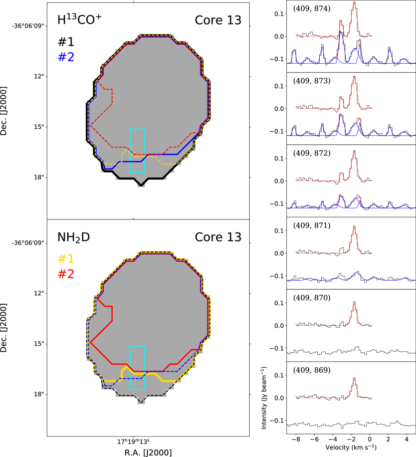
Figure 8: Left: schematic view of decomposed structures identified using the H¹³CO⁺ (upper left) and NH₂D (bottom left) lines for dense core 13. The greyscale is the dense core revealed by the continuum emission. The black and blue contours represent the spatial distributions of the H¹³CO⁺ decomposed structures, while the yellow and red contours represent the spatial distributions of the NH₂D decomposed structures. The contours are derived by the emission regions of corresponding velocity components, while #1 and #2 represent the first and second velocity components, respectively. Right: spectra of the H¹³CO⁺ (upper) and NH₂D (lower) lines within the cyan rectangle shown on the left panel. For the H¹³CO⁺ spectrum, the solid red curve represents the fitted result. For the NH₂D spectrum, the solid blue curve represents the components that are fitted, while solid red curve is the sum of them. The complete figure set (15 images) is available in the online journal.

Figure 9: The gas masses of the H¹³CO⁺ decomposed structures versus that of the NH₂D decomposed structures. The solid red line is the y = x line.

Appendix C Simulation

To examine whether the observed line widths are biased by the spectral resolution or not, we constructed a simplified model. Assuming that the dense cores are in virial equilibrium ($\alpha_{\rm vir}$ = 1), the virial velocity dispersion ($\sigma_{\rm vir}$) can be described by

$$\sigma_{\rm vir}=\sqrt{\frac{\alpha_{\rm vir}\;M_{\rm gas}\;G}{5R}}$$ (C1)

where $M_{\rm gas}$ and $R$ are the gas mass and effective radius. We used the observed line intensity and $\sigma_{\rm vir}$ as input parameters to synthesize a spectrum with a spectral resolution of 0.013 km s^-1 for dense cores (black lines in Figure 10). We fit Gaussian line profiles to the synthetic spectra, that have been smoothed to a spectral resolution of 0.21 km s^-1 and with injected a random noise in 1000 iterations; we only show the dense cores that exhibit a single velocity component in the H¹³CO⁺ emission. Figure 10 shows the fitting results. The fitted line width agrees with the input line width, indicating that the measured line widths are not significantly affected by the current spectral resolution in this study. We ran the same test for the NH₂D line, and reached the same conclusion.

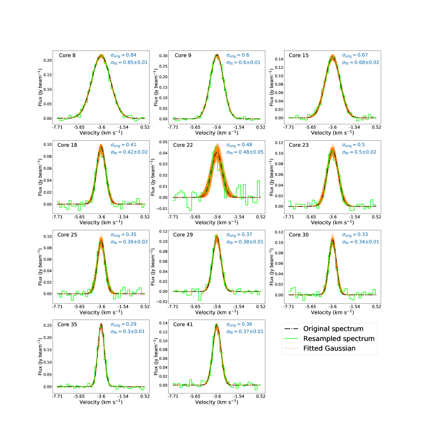
Figure 10: The black line is the original synthesized spectrum in the spectral resolution of 0.013 km s^-1, while the green line is the original synthesized spectrum smoothed to a spectral resolution of 0.21 km s^-1. The yellow lines are fitted results for each iteration. The dense core ID is presented on the upper left panel. The synthesized spectral line width and fitted line width are presented on the upper right panel.

Presented here are individual plots for Figure 8 which are available as the online material. The black cross marks the position of the spectra.

Presented here are individual plots for Figure 8 which are available as the online material.

Presented here are individual plots for Figure 8 which are available as the online material.

Presented here are individual plots for Figure 8 which are available as the online material.

References

- Astropy Collaboration et al. (2013) Astropy Collaboration, Robitaille, T. P., Tollerud, E. J., et al. 2013, A&A, 558, A33
- Bergin & Tafalla (2007) Bergin, E. A., & Tafalla, M. 2007, ARA&A, 45, 339
- Bertoldi & McKee (1992) Bertoldi, F., & McKee, C. F. 1992, ApJ, 395, 140
- Beuther et al. (2002) Beuther, H., Schilke, P., Menten, K. M., et al. 2002, ApJ, 566, 945
- Beuther et al. (2018) Beuther, H., Soler, J. D., Vlemmings, W., et al. 2018, A&A, 614, A64
- Bonazzola et al. (1987) Bonazzola, S., Heyvaerts, J., Falgarone, E., Perault, M., & Puget, J. L. 1987, A&A, 172, 293
- Busquet et al. (2010) Busquet, G., Palau, A., Estalella, R., et al. 2010, A&A, 517, L6
- Butler & Tan (2012) Butler, M. J., & Tan, J. C. 2012, ApJ, 754, 5
- Caselli et al. (2002) Caselli, P., Benson, P. J., Myers, P. C., & Tafalla, M. 2002, ApJ, 572, 238
- Caselli & Myers (1995) Caselli, P., & Myers, P. C. 1995, ApJ, 446, 665
- Chibueze et al. (2014) Chibueze, J. O., Omodaka, T., Handa, T., et al. 2014, ApJ, 784, 114
- Daniel et al. (2016) Daniel, F., Coudert, L. H., Punanova, A., et al. 2016, A&A, 586, L4
- Devereux & Young (1990) Devereux, N. A., & Young, J. S. 1990, ApJ, 359, 42
- Elmegreen & Scalo (2004) Elmegreen, B. G., & Scalo, J. 2004, ARA&A, 42, 211
- Fall & Frenk (1983) Fall, S. M., & Frenk, C. S. 1983, AJ, 88, 1626
- Foster et al. (2009) Foster, J. B., Rosolowsky, E. W., Kauffmann, J., et al. 2009, ApJ, 696, 298
- Friesen et al. (2017) Friesen, R. K., Pineda, J. E., co-PIs, et al. 2017, ApJ, 843, 63
- Ginsburg & Mirocha (2011) Ginsburg, A., & Mirocha, J. 2011, PySpecKit: Python Spectroscopic Toolkit, Astrophysics Source Code Library, , , ascl:1109.001
- Goldsmith (2001) Goldsmith, P. F. 2001, ApJ, 557, 736
- Goodman et al. (1998) Goodman, A. A., Barranco, J. A., Wilner, D. J., & Heyer, M. H. 1998, ApJ, 504, 223
- Hacar et al. (2016a) Hacar, A., Alves, J., Burkert, A., & Goldsmith, P. 2016a, A&A, 591, A104
- Hacar et al. (2016b) Hacar, A., Kainulainen, J., Tafalla, M., Beuther, H., & Alves, J. 2016b, A&A, 587, A97
- Hacar & Tafalla (2011) Hacar, A., & Tafalla, M. 2011, A&A, 533, A34
- Hacar et al. (2017) Hacar, A., Tafalla, M., & Alves, J. 2017, A&A, 606, A123
- Hacar et al. (2018) Hacar, A., Tafalla, M., Forbrich, J., et al. 2018, A&A, 610, A77
- Hacar et al. (2013) Hacar, A., Tafalla, M., Kauffmann, J., & Kovács, A. 2013, A&A, 554, A55
- Heitsch et al. (2009) Heitsch, F., Ballesteros-Paredes, J., & Hartmann, L. 2009, ApJ, 704, 1735
- Hennebelle & Chabrier (2008) Hennebelle, P., & Chabrier, G. 2008, ApJ, 684, 395
- Hildebrand (1983) Hildebrand, R. H. 1983, QJRAS, 24, 267
- Hull & Zhang (2019) Hull, C. L. H., & Zhang, Q. 2019, Frontiers in Astronomy and Space Sciences, 6, 3
- Hunter (2007) Hunter, J. D. 2007, Computing In Science & Engineering, 9, 90
- Joye & Mandel (2003) Joye, W. A., & Mandel, E. 2003, in Astronomical Society of the Pacific Conference Series, Vol. 295, Astronomical Data Analysis Software and Systems XII, ed. H. E. Payne, R. I. Jedrzejewski, & R. N. Hook, 489
- Kauffmann et al. (2008) Kauffmann, J., Bertoldi, F., Bourke, T. L., Evans, N. J., I., & Lee, C. W. 2008, A&A, 487, 993
- Kauffmann et al. (2013) Kauffmann, J., Pillai, T., & Goldsmith, P. F. 2013, ApJ, 779, 185
- Kirk et al. (2006) Kirk, H., Johnstone, D., & Di Francesco, J. 2006, ApJ, 646, 1009
- Kirk et al. (2017) Kirk, H., Friesen, R. K., Pineda, J. E., et al. 2017, ApJ, 846, 144
- Krumholz & McKee (2005) Krumholz, M. R., & McKee, C. F. 2005, ApJ, 630, 250
- Lada et al. (2008) Lada, C. J., Muench, A. A., Rathborne, J., Alves, J. F., & Lombardi, M. 2008, ApJ, 672, 410
- Larson (1981) Larson, R. B. 1981, MNRAS, 194, 809
- Li et al. (2013) Li, D., Kauffmann, J., Zhang, Q., & Chen, W. 2013, ApJ, 768, L5
- Li et al. (2019a) Li, S., Zhang, Q., Pillai, T., et al. 2019a, ApJ, 886, 130
- Li et al. (2017) Li, S., Wang, J., Zhang, Z.-Y., et al. 2017, MNRAS, 466, 248
- Li et al. (2019b) Li, S., Wang, J., Fang, M., et al. 2019b, ApJ, 878, 29
- Lin et al. (2016) Lin, Y., Liu, H. B., Li, D., et al. 2016, The Astrophysical Journal, 828, 32
- Lin et al. (2017) Lin, Y., Liu, H. B., Dale, J. E., et al. 2017, The Astrophysical Journal, 840, 22
- Liu et al. (2015) Liu, H. B., Galván-Madrid, R., Jiménez-Serra, I., et al. 2015, ApJ, 804, 37
- Liu et al. (2013a) Liu, H. B., Ho, P. T. P., Wright, M. C. H., et al. 2013a, ApJ, 770, 44
- Liu et al. (2012) Liu, H. B., Jiménez-Serra, I., Ho, P. T. P., et al. 2012, ApJ, 756, 10
- Liu et al. (2013b) Liu, H. B., Qiu, K., Zhang, Q., Girart, J. M., & Ho, P. T. P. 2013b, ApJ, 771, 71
- Liu et al. (2019) Liu, H. B., Chen, H.-R. V., Román-Zúñiga, C. G., et al. 2019, ApJ, 871, 185
- Mac Low & Klessen (2004) Mac Low, M.-M., & Klessen, R. S. 2004, Reviews of Modern Physics, 76, 125
- Mac Low et al. (1998) Mac Low, M.-M., Klessen, R. S., Burkert, A., & Smith, M. D. 1998, Physical Review Letters, 80, 2754
- McKee (1989) McKee, C. F. 1989, ApJ, 345, 782
- McKee & Ostriker (2007) McKee, C. F., & Ostriker, E. C. 2007, ARA&A, 45, 565
- McKee & Tan (2003) McKee, C. F., & Tan, J. C. 2003, ApJ, 585, 850
- McMullin et al. (2007) McMullin, J. P., Waters, B., Schiebel, D., Young, W., & Golap, K. 2007, in Astronomical Society of the Pacific Conference Series, Vol. 376, Astronomical Data Analysis Software and Systems XVI, ed. R. A. Shaw, F. Hill, & D. J. Bell, 127
- Monsch et al. (2018) Monsch, K., Pineda, J. E., Liu, H. B., et al. 2018, ApJ, 861, 77
- Motte & André (2001) Motte, F., & André, P. 2001, A&A, 365, 440
- Mueller et al. (2002) Mueller, K. E., Shirley, Y. L., Evans, II, N. J., & Jacobson, H. R. 2002, ApJS, 143, 469
- Murray (2011) Murray, N. 2011, ApJ, 729, 133
- Myers et al. (1986) Myers, P. C., Dame, T. M., Thaddeus, P., et al. 1986, ApJ, 301, 398
- Myers et al. (1991) Myers, P. C., Fuller, G. A., Goodman, A. A., & Benson, P. J. 1991, ApJ, 376, 561
- Myers & Goodman (1988) Myers, P. C., & Goodman, A. A. 1988, ApJ, 329, 392
- Palau et al. (2014) Palau, A., Estalella, R., Girart, J. M., et al. 2014, ApJ, 785, 42
- Pattle et al. (2015) Pattle, K., Ward-Thompson, D., Kirk, J. M., et al. 2015, MNRAS, 450, 1094
- Persi & Tapia (2008) Persi, P., & Tapia, M. 2008, Star Formation in NGC 6334, ed. B. Reipurth, Vol. 5, 456
- Pillai et al. (2011) Pillai, T., Kauffmann, J., Wyrowski, F., et al. 2011, A&A, 530, A118
- Pillai et al. (2007) Pillai, T., Wyrowski, F., Hatchell, J., Gibb, A. G., & Thompson, M. A. 2007, A&A, 467, 207
- Pineda et al. (2015) Pineda, J. E., Offner, S. S. R., Parker, R. J., et al. 2015, Nature, 518, 213
- Pirogov et al. (2003) Pirogov, L., Zinchenko, I., Caselli, P., Johansson, L. E. B., & Myers, P. C. 2003, A&A, 405, 639
- Robitaille & Bressert (2012) Robitaille, T., & Bressert, E. 2012, APLpy: Astronomical Plotting Library in Python, Astrophysics Source Code Library, , , ascl:1208.017
- Russeil et al. (2013) Russeil, D., Schneider, N., Anderson, L. D., et al. 2013, A&A, 554, A42
- Sanhueza et al. (2012) Sanhueza, P., Jackson, J. M., Foster, J. B., et al. 2012, ApJ, 756, 60
- Sanhueza et al. (2017) Sanhueza, P., Jackson, J. M., Zhang, Q., et al. 2017, ApJ, 841, 97
- Schmid-Burgk et al. (2004) Schmid-Burgk, J., Muders, D., Müller, H. S. P., & Brupbacher-Gatehouse, B. 2004, A&A, 419, 949
- Seo et al. (2015) Seo, Y. M., Shirley, Y. L., Goldsmith, P., et al. 2015, ApJ, 805, 185
- Shirley (2015) Shirley, Y. L. 2015, PASP, 127, 299
- Shirley et al. (2002) Shirley, Y. L., Evans, Neal J., I., & Rawlings, J. M. C. 2002, ApJ, 575, 337
- Shirley et al. (2003) Shirley, Y. L., Evans, II, N. J., Young, K. E., Knez, C., & Jaffe, D. T. 2003, ApJS, 149, 375
- Smith et al. (2013) Smith, R. J., Shetty, R., Beuther, H., Klessen, R. S., & Bonnell, I. A. 2013, ApJ, 771, 24
- Sokolov et al. (2018) Sokolov, V., Wang, K., Pineda, J. E., et al. 2018, A&A, 611, L3
- Stone et al. (1998) Stone, J. M., Ostriker, E. C., & Gammie, C. F. 1998, ApJ, 508, L99
- Tobin et al. (2015) Tobin, J. J., Stutz, A. M., Megeath, S. T., et al. 2015, ApJ, 798, 128
- Traficante et al. (2018) Traficante, A., Lee, Y.-N., Hennebelle, P., et al. 2018, A&A, 619, L7
- Urquhart et al. (2015) Urquhart, J. S., Figura, C. C., Moore, T. J. T., et al. 2015, MNRAS, 452, 4029
- van der Tak et al. (2000) van der Tak, F. F. S., van Dishoeck, E. F., Evans, II, N. J., & Blake, G. A. 2000, ApJ, 537, 283
- van der Walt et al. (2011) van der Walt, S., Colbert, S. C., & Varoquaux, G. 2011, Computing in Science and Engineering, 13, 22
- Vasyunina et al. (2011) Vasyunina, T., Linz, H., Henning, T., et al. 2011, A&A, 527, A88
- Vazquez-Semadeni et al. (2000) Vazquez-Semadeni, E., Ostriker, E. C., Passot, T., Gammie, C. F., & Stone, J. M. 2000, in Protostars and Planets IV, ed. V. Mannings, A. P. Boss, & S. S. Russell, 3
- Vázquez-Semadeni et al. (2019) Vázquez-Semadeni, E., Palau, A., Ballesteros-Paredes, J., Gómez, G. C., & Zamora-Avilés, M. 2019, MNRAS, 490, 3061
- Vuong et al. (2003) Vuong, M. H., Montmerle, T., Grosso, N., et al. 2003, A&A, 408, 581
- Vutisalchavakul et al. (2016) Vutisalchavakul, N., Evans, Neal J., I., & Heyer, M. 2016, ApJ, 831, 73
- Wang et al. (2008) Wang, Y., Zhang, Q., Pillai, T., Wyrowski, F., & Wu, Y. 2008, ApJ, 672, L33
- Willis et al. (2013) Willis, S., Marengo, M., Allen, L., et al. 2013, ApJ, 778, 96
- Zhang et al. (2015) Zhang, Q., Wang, K., Lu, X., & Jiménez-Serra, I. 2015, ApJ, 804, 141