Re-purposing Heterogeneous Generative Ensembles with Evolutionary Computation

Abstract.

Generative Adversarial Networks (GANs) are popular tools for generative modeling. The dynamics of their adversarial learning give rise to convergence pathologies during training such as mode and discriminator collapse. In machine learning, ensembles of predictors demonstrate better results than a single predictor for many tasks. In this study, we apply two evolutionary algorithms (EAs) to create ensembles to re-purpose generative models, i.e., given a set of heterogeneous generators that were optimized for one objective (e.g., minimize Fréchet Inception Distance), create ensembles of them for optimizing a different objective (e.g., maximize the diversity of the generated samples). The first method is restricted by the exact size of the ensemble and the second method only restricts the upper bound of the ensemble size. Experimental analysis on the MNIST image benchmark demonstrates that both EA ensembles creation methods can re-purpose the models, without reducing their original functionality. The EA-based demonstrate significantly better performance compared to other heuristic-based methods. When comparing both evolutionary, the one with only an upper size bound on the ensemble size is the best.

1. Introduction

Generative Adversarial Networks (GANs) consist of a set of unsupervised machine learning methods to learn generative models (Goodfellow et al., 2014). They take a training set drawn from a specific distribution and learn to represent an estimate of that distribution. GANs combine a generative network (generator) and a discriminative network (discriminator) that apply adversarial learning to be trained. Thus, the generator learns how to create “artificial/fake” samples that approximate the real distribution, and the discriminator is trained to distinguish the “natural/real” samples from the ones produced by the generator. GAN training is formulated as a minmax optimization problem by the definitions of generator and discriminator loss. Hopefully, the GAN training can converge on a generator that is able to approximate the real distribution so well that the discriminator only provides a random label for real and fake samples.

GANs have been successfully applied to a wide range of applications (Wu et al., 2017; Wang et al., 2019; Pan et al., 2019). However, training GANs is difficult since the adversarial dynamics may give rise to different convergence pathologies (Arjovsky and Bottou, 2017; Arora et al., 2018), e.g. vanishing gradient, gradient explosion, and mode collapse. When gradient pathologies appear, the generator is not able to learn and, if the problem persists, it basically generates noise for the whole training process. Mode(generator) collapse happens when the training converges to a local optimum, i.e. the generator produces realistic fake images that only represent a portion of the real data distribution. Therefore, the GAN has not successfully learned the distribution.

A large body of work is devoted to mitigate these problems and improve GAN training robustness (Chintala et al., 2016; Mao et al., 2017; Gulrajani et al., 2017; Nguyen et al., 2017; Radford et al., 2015). A promising approach is training ensembles of networks (Gulrajani et al., 2017; Grover and Ermon, 2018; Toutouh et al., 2019). The ensemble is created by training multiple instances of a GAN (generator/discriminator) in different ways (e.g., different initialization seeds) and combining them (e.g., randomly drawing samples from any generator in the ensemble).

Machine learning (ML) has been taking advantage of evolutionary computing (EC) to address many different tasks (Alexandropoulos et al., 2019; Jin, 2006). In addition, EC has also been applied to ensembles creation (Abbass, 2003; Larcher and Barbosa, 2019; Islam et al., 2003; Langdon et al., 2002; Liu et al., 2000; Chandra and Yao, 2006; Zhang et al., 2017; Fernandes et al., 2019). In particular, EC and GANs have been studied with Lipizzaner (Al-Dujaili et al., 2018; Schmiedlechner et al., 2018) and Mustangs (Toutouh et al., 2019), which apply a distributed coevolutionary approach to train a population of GANs to create an ensemble of generators. Through the training epochs these methods use an evolutionary algorithm (EA) to learn mixture weights to optimize the quality of the generative models.

Lipizzaner and Mustangs apply common measures to assess the the quality of a generative model, e.g., Inception Score (IS) (Salimans et al., 2016) and Fréchet Inception Distance (FID) (Heusel et al., 2017). FID is widely used in image generation problems since it correlates well with the perceived quality of samples and is sensitive to dropped modes. However, FID is not able to distinguish between different failure cases (Borji, 2019). For example, generative models with competitive results in FID score may produce high quality images but only a subset of them (Sajjadi et al., 2018).

The total variation distance (TVD) is a scalar measure used to assess the capacity of a generative model to cover the real data distribution (Li et al., 2017) by accounting for class balance. In this study, we are concerned with the diversity in the generative models (i.e., mode collapse). It is empirically shown that FID is not correlated with the diversity of the generated samples (Borji, 2019; Sajjadi et al., 2018). Thus, we define two problems to optimize ensembles of generators already trained in terms of FID (quality of the image generated) to obtain high diverse samples, i.e., to re-purpose already trained GANs to optimize TVD: Restricted Ensemble Optimization of GENenrators (REO-GEN) and Non-Restricted Ensemble Optimization of GENenrators (NREO-GEN). The main difference between both problems is the first one is restricted by the specific size (number of generators) of the ensemble and the second does not define the size of the ensemble but an upper bound. Finally, we devised two methods evolutionary algorithm (EA) methods to address them.

The main contributions of this paper are: 1) proposing two optimization problems, REO-GEN and NREO-GEN, to obtain high quality and diverse samples from already trained generative models, 2) proposing different methods to address these optimization problems, 3) and obtaining generative models that maximize the diversity of the high quality generated samples.

Thus, we answer the following research questions:

RQ1::

Is it possible to re-purpose GANs trained in terms of a given objective (e.g., FID) to optimize another objective (e.g., TVD) without requiring applying the high computational cost of GAN training?

RQ2::

How can we create high quality and diverse ensembles?

RQ3::

Can be created ensembles of GANs trained independently?

RQ4::

Can we use EC to create competitive ensembles?

RQ5::

Is there any relation between the ensemble size and the quality of the generative model created to deal with a given problem?

The paper is organized as follows. Section 2 and Section 3 present the related work and the optimization problems, respectively. Section 4 describes the methods devised to address the problems. The experimental setup is in Section 5 and results in Section 6. Finally, conclusions are drawn and future work is outlined in Section 7.

2. Related Work

In this section, we introduce some previous research in the main topics of our study: EC to create ensembles and GAN ensembles.

2.1. Evolutionary Ensemble Learning

In ML, an important approach to improve the performance (e.g., classification or prediction) of the models is to strategically combine/fuse them. This is known as ensemble learning (Zhang and Ma, 2012).

There is a body of work on Evolutionary Ensemble Learning (EEL), i.e., the application of EC to learn ensembles. The main idea is to compensate for the limitations of the models trained with the abilities of the others by combining EC with learning algorithms. Accurate and diverse models are the best candidates to satisfactorily create strong ensembles (Dietterich, 2000). Ensemble creation includes several strategies such as (Al-Sahaf et al., 2019; Alexandropoulos et al., 2019): boosting (Schapire, 1990), cascade generalization (Gama and Brazdil, 2000), and stacking (Wolpert, 1992). Genetic Algorithms (GAs) have been used to successfully create ensembles by multiple ML methods, e.g. Support Vector Machines, Neural Networks (NN), and Genetic Programming (GP) (Pławiak et al., 2019; Zhou et al., 2002; Padilha et al., 2016; Sohn and Yoo, 2019).

GP has been used as a base learner for classification or regression problems. Moreover, GP has been used to improve such a models by creating ensembles (Bhowan et al., 2011; Mauša and Grbac, 2017; Folino et al., 2006; Fitzgerald et al., 2013; Folino et al., 2003; Iba, 1999). A bagging method based on GP has been applied to ensemble Interval GP (IGP) classifiers that are independently trained (i.e., performing different runs) (Tran et al., 2018). The experimental analyses have shown that this new method is able to outperform single IGP and different types of ensembles. In order to reduce the computational complexity of ruining GP training methods to obtain the models, a method based on a spatial structure with bootstrapped elitism (SS+BE) has been presented (Dick et al., 2018). This method is able to generate an ensemble from a single run.

Multi-objective (MO) GP has been applied to build an ensemble of classifiers with unbalanced data, which competing objectives are the minority and majority class accuracy (Bhowan et al., 2011). Other MO approaches have been applied to generate ensembles (Ribeiro and Reynoso-Meza, 2018; Bi et al., 2019). For example, Pareto Differential Evolution (PDE) has been used to evolve an ensemble of NN using negative correlation learning (NCL) in the fitness to increase ensemble diversity (Abbass, 2003). PDE and Nondominated Sorting GA-II (NSGA-II) have been similarly applied to evolve NN ensembles. In this case, the training accuracy is traded off against the diversity of the evolved models, measured using the NLC of the ensemble members (Chandra and Yao, 2006).

There is also a lot of research about applyingapplying Evolutionary Strategies (Lima et al., 2013; Schmiedlechner et al., 2018; Toutouh et al., 2019), Particle Swarm Optimization (Pulido et al., 2016; Aburomman and Reaz, 2016; Ripon et al., 2020) or Ant Colony Optimization (Meng and Xu, 2018; Ripon et al., 2020).

2.2. GAN Ensemble Models

Recently, a number of variants of GANs have raised to address training issues suffered by the seminal approach presented by Goodfellow (Goodfellow et al., 2014). Inspired by the works that propose creating ensembles of convolutional neural networks (CNNs) as a straightforward way to improve results (Krizhevsky et al., 2012; Chen et al., 2019), several authors have proposed similar solutions to deal with GAN learning pathologies. Many GAN methods have been proposed for remedying the convergence pathologies of GAN training by creating mixtures(ensembles) of GANs (Gulrajani et al., 2017; Wang et al., 2016; Tolstikhin et al., 2017; Grover and Ermon, 2018; Hoang et al., 2017; Durugkar et al., 2016).

EC has been also applied to generate ensembles of GANs. Lipizzaner (Al-Dujaili et al., 2018; Schmiedlechner et al., 2018) and Mustangs (Toutouh et al., 2019) train a spatially distributed population of GANs. Sub-populations (neighborhoods) of GANs apply a competitive coevolutionary algorithm to adversarially train the generators and the discriminators. The main motivation behind Lipizzaner is to maintain diversity in order to improve the robustness of GAN training. At the end of each epoch, these algorithms apply a number of generations of the Evolutionary Strategies (ES) algorithm (Loshchilov, 2013) to evolve the mixture weights used to define the ensemble of generators defined by the sub-populations to maximize the quality of the generated samples (e.g., to optimize IS or FID).

Thus, the main motivation of this research is to define a novel method to re-purpose (or to improve) GANs by coupling concepts coming from EEL and GANs training. The aim is to fill the gap that exists in addressing GAN training issues by applying a methodology motivated by the successful EEL. This methodology can obtain more competitive new generative models by combining heterogeneously trained generators, without requiring the high computational cost of re-training new GANs.

3. Output Diversity GAN Optimization

The goal of this study is to re-purpose generative models to allow them to generate samples according to a new objective function. We focus on optimizing TVD (diversity) of GANs that have been optimized to get high quality images in terms of FID. Eq. 1 defines TVD applied to assess the class balance (i.e., diversity of the samples generated), lower TVD means more diverse samples.

(1) $$\small TVD=\frac{1}{2}\sum_{c\in Classes}{\mid freq(real_{c})-freq(fake_{c})\mid}$$

In general, the quality of the generative models is assessed by using one-dimensional metrics (e.g., IS and FID) that are not able to measure the diversity of the samples (Sajjadi et al., 2018). We empirically evaluated the correlation between FID and TVD scores of 700 generators trained to generate digits of MNIST dataset (LeCun, 1998) by creating 50,000 images from each generator. The generators with high quality (FID$<$40) have a Spearman’s correlation coefficient between FID and TVD of 0.2, i.e. no correlation. Thus, when FID is being optimized does not mean that TVD is also being improved. This motivates the optimization of TVD for generators that have been optimized on FID. We have defined REO-GEN and NREO-GEN to create ensembles of generators that maximize the diversity (i.e., minimize TVD) without worsening the FID.

Given a set of trained generators $\mathbf{G}=\{g_{0},...,g_{n-1}\}$. We define the ensemble optimization problem as to find the $n$-dimensional mixture weight vector $\bm{w}$ that is defined as follows

(2) $$\footnotesize\bm{w}^{*}=\operatorname*{arg\,min}TVD\big{(}\sum_{0\leq i<s}w_{i}G_{g_{i}}\big{)}\;,$$

where $w_{i}$ represents the probability that a data sample comes from the $i$th generator in $\mathbf{G}$ and $G_{g_{i}}$ represents the samples created by $g_{i}$, with $\sum_{w_{i}\in\bm{w}}w_{i}=1$. REO-GEN applies the restriction that the ensemble size $s$ is known, and therefore, $|w_{i}\neq 0|=s$ (i.e., number of mixture weights different to 0 are $s$). In contrast, NREO-GEN relaxes the restriction by defining an upper bound for the size, $|w_{i}\neq 0|\leq s$.

4. Genetic Ensemble Creation

In order to address REO-GEN and NREO-GEN problems, we apply two evolutionary approaches based on GA. We use two different solutions representations to deal with the difference between these two variants of the problem (e.g., fixed size and variable size of the ensemble) Subsequently, we also have two different types of evolutionary operators to complement their encoding.

The solutions are randomly initialized keeping the values in the correct range according to the representation (see sections 4.1.1 and 4.2.1), the recombination operators are versions of the two point crossover, and ad hoc mutation operators are specifically devised for these problems. In the following subsections, we present them, as well as the objective (fitness) function evaluation.

4.1. REO-GEN Encoding and Operators.

This section describes the solution encoding and the evolutionary operators applied to address REO-GEN by using a GA.

4.1.1. REO-GEN Encoding

A solution is represented as a vector of real numbers with two decimals of precision, having length $s$ (size of the ensemble). Thus a solution $\mathbf{e}$ is represented by $\mathbf{e}=\langle g^{0}.w^{0},\dots,\ g^{s-1}.w^{s-1}\rangle$. The integer part $g^{i}$ of these real numbers identifies the generator in the ensemble, where $g^{i}\neq g^{j}$ for $i\neq j$ The probability of using $g^{i}$ to draw a sample is given by the two digits of the fractional part ($w^{i}$). Thus, we have the following restrictions: having $n$ pre-trained models $g^{i}\in\{0,...,n-1\}$, $w^{i}\neq 0$, and $\sum^{0\leq i<s}w_{i}=100\%$.

Figure 1 solutions for two different problem instances defined by different ensemble sizes: $e_{i}$ and $e_{j}$. The first one represents a vector $\langle 5.13,\ 2.15,\ 0.72\rangle$ that encapsulates an ensemble of size three which is made of generators identified with numbers 5, 2, and 0 that draw samples with probabilities 0.13, 0.15, and 0.72, respectively. The second one shows an ensemble of size four built with generators identified with numbers 4, 1, 2, and 5 that draw samples with probabilities 0.22, 0.16, 0.22, and 0.19, respectively.

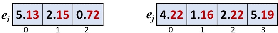
Figure 1. REO-GEN solution representation examples.

4.1.2. REO-GEN Recombination

From the parents ($e_{i}$ and $e_{j}$), the offspring ($e_{i+1}$ and $e_{j+1}$) are generated by exchanging information of the genes (with index $c$) located between two randomly selected points within the chromosome. The operator swaps the integer part of the real numbers (i.e., it exchanges the generators identifier $g^{c}_{i}$ and $g^{c}_{j}$) and it averages the weights (i.e., $w^{c}_{i}$,$w^{c}_{j}$=$\frac{w^{c}_{i}+w^{c}_{j}}{2}$). Figure 2 shows an example of the application of this recombination operator.

After applying the recombination a fixing operator is applied to fix duplicate of generators and to keep the solution under restriction $\sum^{0\leq i<s}w_{i}=100$. It avoids duplicate generators $g_{i+1}^{c}$ (if there is some) by keeping the new occurrence of that generator (i.e., the one that came from the other parent) and changing the old one by the generator that was encoded in $g_{i}^{c}$. After swapping generators in Figure 2, $g_{i+1}^{2}$=$g_{i+1}^{3}$=5, the solution is fixed by $g_{i+1}^{3}$=$g_{i}^{2}$=2. The weights are fixed by keeping the same proportions after computing the new weights, but normalizing them to sum 100.

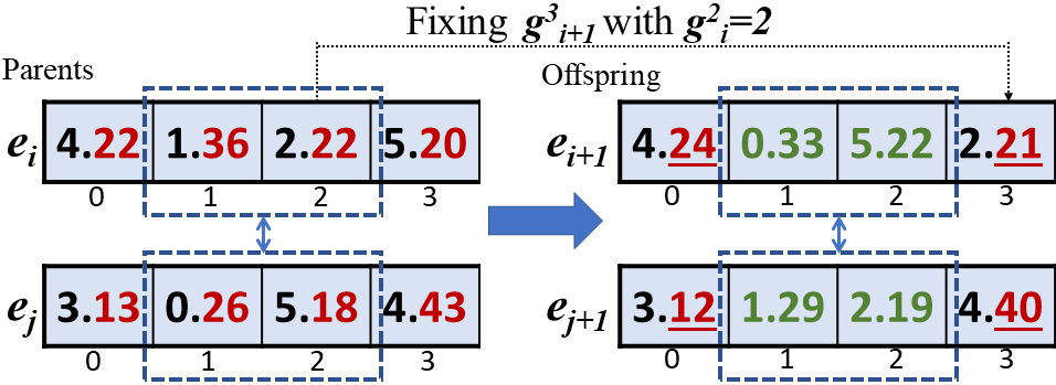
Figure 2. REO-GEN crossover/recombination example.

4.1.3. REO-GEN Mutation

The mutation operator equally likely applies three variations on solutions (see Figure 3). These variations work as follows: 1) changing the generatorin the mutated gene with a randomly selected one of the ones not included in the ensemble; 2) modifying the probabilitiesof the mutated gen $w^{c}_{i}$ and another one randomly selected $w^{d}_{i}$ by adding or subtracting a random value (doing the opposite operation in the other gen) keeping the sum of probabilities in 100 and $w^{c}_{i},w^{d}_{i}>0$; and 3) combining both, the generator and the weight mutations (mutation 1 and 2).

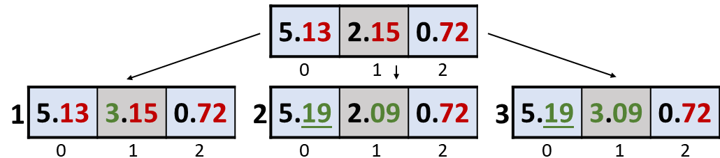
Figure 3. REO-GEN mutation examples.

4.2. NREO-GEN Encoding and Operators.

This section describes the solution encoding and the evolutionary operators applied to address NREO-GEN by applying a GA.

4.2.1. NREO-GEN Encoding

Solutions are represented as vectors of integer numbers divided in three segments: ensemble size (one element), generators identification ($n$ elements), and probability definition ($n$ elements); having length $2n+1$. The ensemble $\mathbf{e}$ is represented by $\mathbf{e}=\langle e^{0},e^{1},\dots,e^{n},e^{n+1},\dots,e^{2n}\rangle$. The first element of the vector defines the size of the ensemble, i.e, $e^{0}<n$. The following $n$ elements (generators identification segment) identify the $n$ pre-trained generators, which identifiers are randomly shuffled and located when the GA initializes the solution. The last $n$ elements represent the probabilities of using the generators in the same order specified in the generators identification segment, i.e., $e^{n+i}$ element of the vector encapsulates the probability of using the generator identified in the $e^{i}$ (i.e., $w_{i}$=$e^{n+i}/100$).

Thus, we have the following restrictions: $e^{i}\neq e^{j}$ for $i,j\in\{1,...,n\}$ if $i\neq j$ (i.e., there is not any repetition in the generators identification segment of the vector), $e^{i}\neq 0$ $i\in\{n+1,...,e^{0}\}$ (i.e., all probabilities are higher than 0), and $\sum_{n+1\leq i<n+e^{0}}e^{i}=100$.

Figure 4 illustrates two examples of solutions, $e_{i}$ and $e_{j}$, in a problem to create ensembles from six pre-trained generators. The first one represents an ensemble with three generators: generators identified with numbers 5, 2, and 0 that draw samples with probabilities 0.13, 0.15, and 0.72 of the samples, respectively. The second one hast four generators: 4, 1, 2, and 5, with the following probabilities: 0.22, 0.16, 0.43 and 0.19.

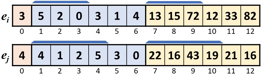
Figure 4. NREO-GEN solution representation examples.

4.2.2. NREO-GEN Recombination

The offspring ($e_{i+1}$ and $e_{j+1}$) are generated by swapping the generators and the weights between two points in both vector segments of the parents, $e_{i}$ and $e_{j}$ (see Figure 5). The two points are selected within the range of the size of the smallest ensemble.

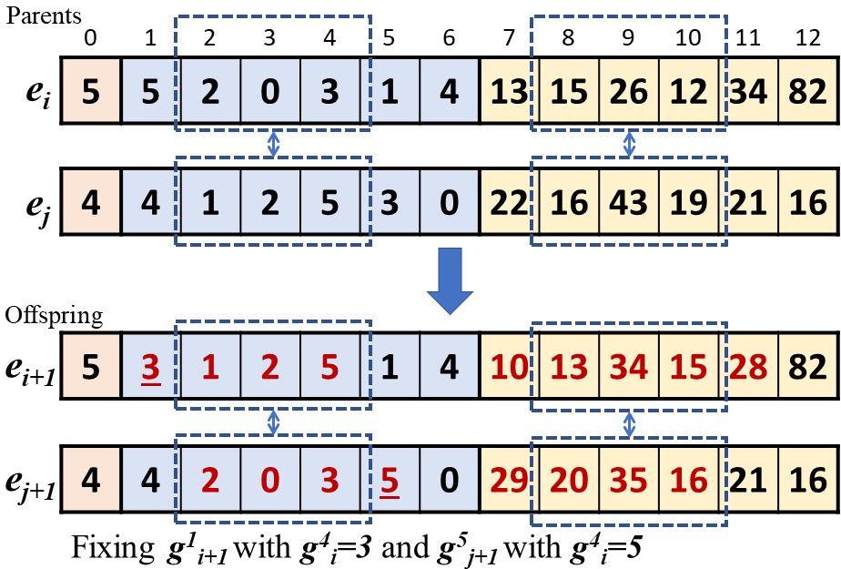
Figure 5. NREO-GEN crossover/recombination example.

Figure 5 shows an example of applying recombination to $e_{i}$ and $e_{j}$ solutions. As the smallest ensemble ($e_{j}$) has size four, the two points for swapping the gens will be randomly picked between one and four. In this example, the two points are two and four. If after the recombination a solution has a generator duplicated, the fixing operator is applied. The genetic information that has just come from the other parent is kept and the old occurrence of that generator is changed for some generator that will be missing in the ensemble. The underlined generators in Figure 5 (i.e, generator 3 in $e_{i}$ and 5 in $e_{j}$) have been modified to avoid generators repetition. If the sum of weights is not 100 (i.e., $\sum_{n+1\leq i<n+e^{0}}e^{i}\neq 100$), the probability definition is fixed, too. As in REO-GEN recombination, the weights are fixed by keeping the same proportions after computing the new weights, but normalizing them to sum 100.

4.2.3. NREO-GEN Mutation

The mutation operator equally likely applies four variations on solutions (see Figure 6). These variations work as follows: 1) exchanging a generatorin the ensemble with another one that is not included; 2) mutating the probabilitiesby exchanging the mutated gen and another one in the probabilities definition segment (within the range of $n$ and $n$+$e^{0}$) by adding or subtracting a random value (doing the opposite operation in the other gen) keeping the sum of the probabilities being 100; 3) mutating both, the generator and the weight; and 4) changing the ensemble size, which requires updating the probabilities in the way that they sum 100, but keeping proportional probabilities.

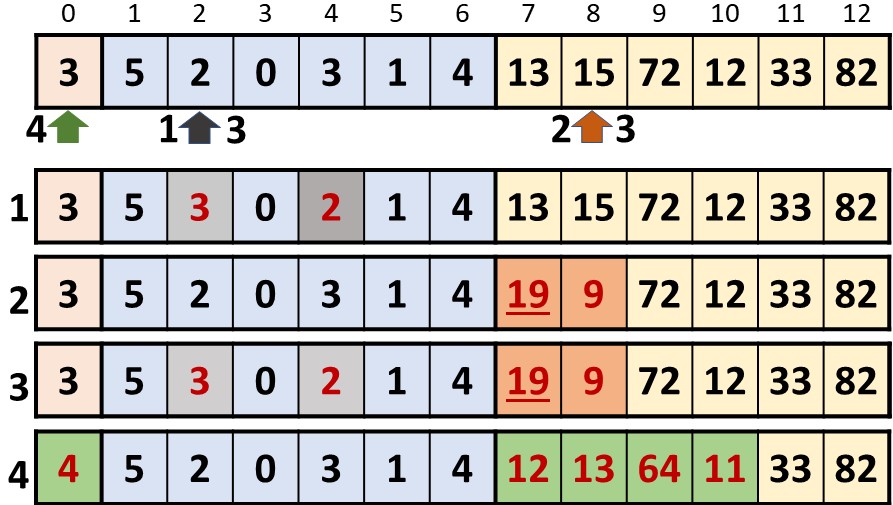
Figure 6. NREO-GEN mutation examples.

4.3. REO-GEN and NREO-GEN Solutions Evaluation

The solutions are evaluated by drawing a number of samples (images) by using the ensemble represented in the chromosome and assessing the resulted TVD, i.e., fitness($e_{i}$)=TVD($e_{i}$). As stated in Section 3, this is a minimization problem.

5. Experimental Analysis

This section details the experimental analysis performed to evaluate the evolutionary generative ensemble creators proposed to improve output diversity.

5.1. Implementation and Execution Platform

The experiments are performed on a cloud that provides 16 Intel Cascade Lake cores up to 3.8 GHz with 64 GB RAM and a GPU which are either NVIDIA Tesla P4 (8 GB RAM) or NVIDIA Tesla P100 (16 GB RAM). All methods have been implemented in Python3 using pytorch and DEAP (Distributed Evolutionary Algorithms in Python) (Kim and Yoo, 2019) libraries. The source code implemented is public.

5.2. Problem Instance – MNIST

We use the common dataset from the GAN literature: MNIST (LeCun, 1998), which consists of low dimensional handwritten digits images. We have had access to a pool of 700 GANs trained by using several different methods. After evaluating them in terms of FID and TVD, we filter out low-quality generators, we pick quality based on results of previous GAN studies based on MNIST, i.e., $FID<40$. Applying the threshold, we get 220 different generators with average FID of 36.393 and average TVD of 0.113. Finally, we address REO-GEN and NREO-GEN to compute ensembles that optimize TVD constructed from this set of 220 generators.

We define different experiments for REO-GEN and NREO-GEN. First, we address the problem for ensembles sizes between three and 10 (number of classes in MNIST). For NREO-GEN, we perform two different experiments, one addressing the problem with a maximum of eight generators in the ensemble, and the second one, with a maximum of 100 (the max ensemble size in the current implementation, 100 generators with a minimum probability of 0.01).

5.3. Baseline Methods

To evaluate the quality of the solutions from our EAs we implemented two versions of a constructive heuristic to solve variants of the REO-GEN problem, named Iterative Greedy (IG) and Random Greedy (RG). Both methods start by sorting the generators according to the quality of the images generated (i.e, FID). The identifier of the sorted generators are stored on a vector $\mathbf{G^{FID}}$=$\langle g^{FID}_{0},\dots,g^{FID}_{n-1}\rangle,g^{FID}_{i}\leq g^{FID}_{i+1},i\in[0,n]$, which the first element is the generator with the best FID.

Once the generators are sorted, IG applies a constructive heuristic to select the generators and their weights to create an ensemble of size $s$, defined by two vectors $\mathbf{G^{FID}_{o}}$ that contains the generators’ identifiers and $\mathbf{W^{FID}_{o}}$ that includes the weights (see Algorithm 1).

The heuristic starts by evaluating the TVD of the current ensemble, which is defined by just one generator, i.e., $\mathbf{G^{FID}_{o}}=\langle g^{FID}_{0}\rangle$ and $\mathbf{W^{FID}_{o}}=\langle 1.00\rangle$ (line 4). Then, IG iterates over $\mathbf{G^{FID}}$ starting by the second generator to create an ensemble.

For each iteration $i$ a new generator $g^{FID}_{i}\in$ $\mathbf{G^{FID}}$ is considered to be part of the optimal ensemble, see line 7 (i.e., it creates an auxiliary ensemble $\mathbf{G}$ by adding $g^{FID}_{i}$ to $\mathbf{G^{FID}_{o}}$). Then, IG iteratively tests all the possible combinations of weights $\mathbf{W}$ that belong to $\mathbf{W^{g}}$ for the generators in $\mathbf{G}$, where $\mathbf{W^{g}}$=$\{0.0,0.1,0.2,0.3,0.4,0.5,0.6,0.7,0.8,0.9\}$ to limit the possible combinations of weights and considering that all the combinations satisfy the restriction $\sum_{w_{i}\in\mathbf{W}}w_{i}=1$. It evaluates the TVD of all the tentative generative models defined by the generators in $\mathbf{G}$ and all the combinations in $\mathbf{W}$ (line 10). If the best tentative ensemble has better TVD than the best ensemble found so far defined by $\mathbf{G^{FID}_{o}}$ and $\mathbf{W^{FID}_{o}}$, these ensemble is considered the new best ensemble found so far. In contrast, if the best TVD of the new ensemble is lower, $g^{FID}_{i}$ is not considered to be part of $\mathbf{G^{FID}_{o}}$ (line 11).

At the end of each iteration $i$, if there are any generators with weight equal to 0, these generators are not considered as a part of the ensemble and they are removed from the current solution, i.e., $\mathbf{G^{FID}_{o}}$ (line 15). This iterative method finishes when the size of the best ensemble found so far is $s$, i.e., $|\mathbf{G^{FID}_{o}}|=|\mathbf{W^{FID}_{o}}|=s$.

Algorithm 1 Iterative Greedy
Input:  $G$: Set of generators, $W^{g}$: Set of possible weights, $s$: Size of ensemble
Return:  $\mathbf{G^{FID}_{o}}$: Generators in ensemble,  $\mathbf{W^{FID}_{o}}$: Weights in ensemble

1:$\mathbf{G^{FID}_{o}}\leftarrow$ sortGenerators($G$) $\triangleright$ Sort generator by FID

2:$\mathbf{G^{FID}_{o}}\leftarrow\langle g^{FID}_{0}\rangle$ $\triangleright$ First element of the ensemble, the best generator

3:$\mathbf{W^{FID}_{o}}\leftarrow\langle 1.00\rangle$

4:$bestTVD\leftarrow$ evaluateTVD($\mathbf{G^{FID}_{o}},\mathbf{W^{FID}_{o}}$) $\triangleright$ Evaluate TVD

5:$i\leftarrow 1$ $\triangleright$ Initialize counter

6:while sizeOf($\mathbf{G^{FID}_{o}}$)$<s$ and $i<|G|$ do$\triangleright$ Loop over generators

7:    $\mathbf{G}\leftarrow$ addGenerator$(\mathbf{G^{FID}_{o}},g_{i}^{FID})$ $\triangleright$ Add $g_{i}^{FID}$ to $\mathbf{G^{FID}_{o}}$

8:    for $\mathbf{W}$ $\in$ allPossibleCombinations($\mathbf{G},W^{g}$) do

9:$\triangleright$ Iterate through all possible weights

10:         $TVD\leftarrow$ evaluateTVD($\mathbf{G},\mathbf{W}$) $\triangleright$ Evaluate TVD

11:         if $TVD<bestTVD$ then$\triangleright$ Replace if new ensemble is better

12:             $bestTVD\leftarrow TVD$

13:             $\mathbf{G^{FID}_{o}}\leftarrow\mathbf{G}$

14:             $\mathbf{W^{FID}_{o}}\leftarrow\mathbf{W}$              

15:    $\mathbf{G^{FID}_{o}}\leftarrow$ fixEnsemble($\mathbf{G^{FID}_{o}}$) $\triangleright$ Remove generators with weights 0

16:    $i\leftarrow i+1$

RG applies the same method, but in each iteration, it randomly picks the new generator $g^{FID}_{r}$ to be added to $\mathbf{G^{FID}_{o}}$, instead of iterating over $\mathbf{G^{FID}}$. The only restriction is $g^{FID}_{r}\notin\mathbf{G^{FID}_{o}}$. Additionally, two random search methods are applied to address both REO-GEN and NREO-GEN, named Random REO Search (RRS) and Random NREO Search (RNRS) respectively. They randomly generate a number of ensembles and return the ensemble with the best TVD.

5.4. Experimental setup

The solutions are evaluated by generating 50,000 samples (images) to get a robust result of the non-deterministic TVD evaluation. The stop condition of the GA and random search methods is performing 10,000 of fitness (TVD) evaluations. The GA is configured to evolve a population of 100 ensembles. The stop condition of the heuristic methods, IG and RG, is given by finding the ensemble of the required size ($s$). Although IG applies an iterative deterministic method, the algorithm does not return the same result every independent run because it relies on the stochastic evaluation of the TVD. Moreover, this has an effect on the number of evaluations required to construct the ensemble, which may be different even for the same ensemble size. Thus, we perform 30 independent runs of each experiment (methods and ensemble sizes). To assess the statistical significance, as the results are not normally distributed, we perform Wilcoxon statistical tests (fixing p-value$<$0.01).

In addition, to compare against the heuristics for different ensemble sizes, we also report the output of RRS and GA when performing a “similar” number of fitness evaluations. The stop condition, in this case, is the average number of fitness evaluations performed by both greedy methods, which is different for each ensemble size. In the tables, these results are identified with a triangle ($\blacktriangledown$) in the name of the algorithm, i.e., RRS$\blacktriangledown$ and GA$\blacktriangledown$.

Finally, owing to the stochastic nature of EAs, a parameter configuration is mandatory prior to the experimental analysis. We performed an experimental analysis to configure two important parameters of the GA: the recombination probability ($p_{r}$) and the mutation probability ($p_{m}$). For each parameter, three candidate values were tested: $p_{r}\in\{0.25,0.50,0.75\}$ and $p_{m}\in\{0.01,0.05,0.1\}$. We keep the configuration that computed the best results.

6. Results and Discussion

This section discusses the main results of the experiments carried out to evaluate the evolutionary GAN ensembles creation problem by addressing REO-GEN and NREO-GEN.

6.1. Final Fitness (TVD)

Tables 1 and 2 summarize the results by showing the best fitness (TVD) for the different methods and ensemble sizes in the 30 independent runs for REO-GEN and NREO-GEN, respectively. These results are not normally distributed. Thus, the tables present the best solution found (Min), the median value (Median), the interquartile range (Iqr), and the least competitive result (Max).

Table 1. REO-GEN final fitness (TVD). Best value is bold.

Method	Min (Best)	Median	Iqr	Max
Ensemble size ($s$): 3
IG	0.067	0.074	0.005	0.086
RG	0.055	0.069	0.014	0.089
RRS$\blacktriangledown$	0.048	0.064	0.014	0.074
GA$\blacktriangledown$	0.053	0.062	0.006	0.071
RRS	0.036	0.046	0.004	0.051
GA	0.030	0.046	0.011	0.061
Ensemble size ($s$): 4
IG	0.056	0.066	0.005	0.073
RG	0.045	0.065	0.010	0.079
RRS$\blacktriangledown$	0.047	0.060	0.008	0.067
GA$\blacktriangledown$	0.034	0.052	0.008	0.062
RRS	0.038	0.046	0.004	0.052
GA	0.030	0.039	0.005	0.050
Ensemble size ($s$): 5
IG	0.047	0.063	0.007	0.071
RG	0.044	0.063	0.018	0.096
RRS$\blacktriangledown$	0.040	0.053	0.006	0.067
GA$\blacktriangledown$	0.034	0.046	0.005	0.062
RRS	0.036	0.047	0.007	0.064
GA	0.033	0.042	0.008	0.056
Ensemble size ($s$): 6
IG	0.054	0.060	0.007	0.075
RG	0.040	0.050	0.012	0.063
RRS$\blacktriangledown$	0.042	0.049	0.004	0.053
GA$\blacktriangledown$	0.036	0.044	0.007	0.055
RRS	0.042	0.048	0.003	0.053
GA	0.033	0.043	0.008	0.055
Ensemble size ($s$): 7
IG	0.046	0.057	0.003	0.070
RG	0.030	0.050	0.007	0.062
RRS	0.035	0.047	0.006	0.052
GA	0.035	0.043	0.005	0.050
Ensemble size ($s$): 8
RRS	0.036	0.047	0.006	0.053
GA	0.036	0.044	0.006	0.050
Ensemble size ($s$): 9
RRS	0.034	0.047	0.004	0.053
GA	0.031	0.044	0.007	0.054
Ensemble size ($s$): 10
RRS	0.042	0.048	0.004	0.054
GA	0.037	0.044	0.005	0.053

Focusing on REO-GEN results in Table 1, we observe that for the ensemble sizes 8, 9, and 10, there are no results from the heuristic methods because of computational cost restrictions. Additionally, for size 7, there are no results of GA$\blacktriangledown$ and RRS$\blacktriangledown$ because the heuristics on average performed 17,630 fitness evaluations ($>>$10,000). GA obtained the best results in terms of the median value for all ensemble sizes. Wilcoxon statistical analysis confirms that GA is the best method for all ensemble sizes.

When evaluating the second most competitive algorithm, there are two cases: first, GA$\blacktriangledown$ is reported (ensemble sizes from 3 to 6), and second, there is not GA$\blacktriangledown$ (ensemble sizes from 7 to 10). In the first case, RRS gets the second-best results for small ensembles sizes (3 and 4), i.e, a very limited number of fitness evaluations, and GA$\blacktriangledown$ is the second-best for ensemble sizes of 5 and 6. As GA$\blacktriangledown$ performs more generations, it converges to better solutions. Thus, the evolutionary operators guide GA to more competitive results than RRS requiring a lower computational cost. In the second case, RRS keeps being the second most competitive.

Regarding the best ensemble found (minimum TVD), similar results are obtained: GA is the most competitive except for ensemble size 7. RG finds the best ensemble so far that size (TVD=0.030), but it required an average of 17,630 fitness evaluations.

Regarding the methods with similar computational cost (i.e., IG, RG, RRS$\blacktriangledown$, and GA$\blacktriangledown$), GA$\blacktriangledown$ obtains the best median value and the best minimum (except for the smallest ensemble).

Focusing NREO-GEN results in Table 2, we can clearly state that GA significantly outperforms RRS in both types of experiments. These results are confirmed by the Wilcoxon statistical test (i.e., p-value$<<$0.01). GA solving the second variant of the problem provides significantly better results than when addressing REO-GEN.

Table 2. NREO-GEN final fitness (TVD). Best value is bold.

Method	Min (Best)	Median	Iqr	Max
Maximum ensemble size: 8
RRS	0.045	0.050	0.004	0.056
GA	0.025	0.034	0.007	0.042
Maximum ensemble size: 100
RRS	0.048	0.052	0.003	0.059
GA	0.026	0.035	0.006	0.042

The results obtained by using GA to address REO-GEN and NREO-GEN allow us to answer RQ4: Can we use EC to create better ensembles? Yes, EC can be used to create better generative models that are able to be re-purposed to optimize a new objective (TVD).

6.2. Fitness (TVD) Evolution

Figure 7 shows the evolution of fitness during the independent run that returns the median fitness. We evaluated that for GA addressing REO-GEN (for all values of $s$) and NREO-GEN, which in the figure are named GA-REO(s), GA-NREO(8), respectively.

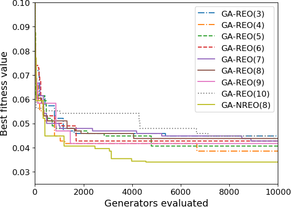
Figure 7. Fitness evolution of the median run.

We can see in Figure 7 that GA-NREO(8) converges faster than the other methods to ensembles with low TVD. It converges to the best ensemble before the first 5,000 fitness evaluations. When analyzing the fitness evolution of the GA addressing REO-GEN, when $s$=10 the algorithm converges slower and it converges to the least competitive results (to the same results than ensembles of size 3). For the other ensemble sizes, the performance is similar. However, for the ensemble size $s$=4, the fitness converges to the best results of the GA-REO(s). This is consistent with the results in Table 1, where the best results are provided by GA for $s$=4.

6.3. Comparison between Optimizers

In order to compare the different methods, we evaluate the generative models returned in each independent run by GA and RRS when solving REO-GEN (for all values of $s$) and the ones computed by GA when addressing NREO-GEN (with a maximum size of 8). Thus, we compute the percentage of improvement in the TVD of method $A$ over method $B$ by evaluating $\Delta(A,B)$=$\frac{TVD(B)-TVD(A)}{TVD(B)}\%$ for the same ensemble size. Additionally, we performed Wilcoxon statistical tests to assess statistical significance. Table 3 presents the results of evaluating $\Delta$. A diamond $\diamond$ is used to specify that there is statistical significance (i.e., $\alpha<0.01$).

Table 3. Delta between methods in different ensemble sizes.

Ensemble	GA-REO(s) vs	GA-NREO(8) vs	GA-NREO(8) vs
size ($s$)	RRS-REO(s)	RRS-REO(s)	GA-REO(s)
3	-1.12%	$\diamond$ 37.81%	$\diamond$ 39.37%
4	$\diamond$ 14.42%	$\diamond$ 37.19%	$\diamond$ 19.90%
5	$\diamond$ 14.56%	$\diamond$ 46.30%	$\diamond$ 27.71%
6	$\diamond$ 9.62%	$\diamond$ 42.50%	$\diamond$ 30.00%
7	$\diamond$ 7.64%	$\diamond$ 39.37%	$\diamond$ 29.48%
8	$\diamond$ 5.75%	$\diamond$ 37.92%	$\diamond$ 30.42%
9	$\diamond$ 8.20%	$\diamond$ 41.98%	$\diamond$ 31.23%
10	$\diamond$ 7.81%	$\diamond$ 45.21%	$\diamond$ 34.69%

As it can be seen in Table 3, when comparing GA-REO(s) and RRS-REO(s). The first one is always statistically better than RRS-REO(s) for all ensemble sizes, except for the smallest ensemble ($s$=3) in which GA lightly worsen the results of the random search. As shown in Figure 7, for this ensemble size the GA converges to the least competitive fitness values. The best improvements of GA-REO(s) over RRS-REO(s) are obtained for ensembles of size 4 and 5. The improvements of GA-NREO(8) over RRS-REO(s) that are shown in the third column of Table 3 are very significant ($>$37%). The same occurs when we compare the ensembles obtained by this evolutionary approach and the GA solving REO-GEN. The ones got by the first one are statistically better for all ensemble sizes.

With these results we can answer RQ2: How can we create high quality and diverse ensembles? The best way to obtain a generative model based on ensembles to create the digits of MNIST is by solving NREO-GEN by using GA. The grade of freedom of GA when solving NREO-GEN allows the method to explore better the search space to find diverse and better (high quality) solutions.

6.4. Generative Models Quality

In this section, we evaluate the performance of the generative models obtained in terms of TVD and FID. But, before we evaluate the shape (number of generators) of the generative models returned by GA when it addresses NREO-GEN since we observe that the best generator size for solving REO-GEN is $s$=4 (see Section 6.1). Table 4 shows the percentage of solutions given the size of the ensemble.

Table 4. Delta between methods in different ensemble sizes.

Ensemble size	3	4	5	6	7	8
Percentage of solutions ($\%$)	23.3	46.7	20.0	6.7	0.0	3.3

According to the results in Table 4, the most repeated size of a final solution given by GA is 4. Thus, this method likely converges to ensembles with the size of the most competitive results addressing REO-GEN, but obtaining more competitive TVD.

Table 5 presents the mean (Mean) and standard deviation (Stdev) of the TVD and FID obtained by the ensembles returned by RRS and GA for each value of $s$. Moreover, we report the same metrics for the ensembles computed by GA addressing NREO-GEN (last row). The results of individually evaluating the 220 generators used to define the problem instance are shown in the first row.

Table 5. Quality of samples according to the ensemble size.

Ensemble size ($s$)	TVD	FID
	Mean$\pm$Stdev	Mean$\pm$Stdev
1	0.113$\pm$0.010	36.393$\pm$1.985
3	0.046$\pm$0.006	27.576$\pm$3.947
4	0.043$\pm$0.005	27.890$\pm$3.048
5	0.046$\pm$0.007	28.225$\pm$3.888
6	0.045$\pm$0.005	27.077$\pm$3.030
7	0.045$\pm$0.005	27.556$\pm$3.531
8	0.046$\pm$0.005	26.726$\pm$3.515
9	0.046$\pm$0.005	26.919$\pm$3.181
10	0.047$\pm$0.004	27.218$\pm$3.408
GA-NREO(8)	0.033$\pm$0.004	27.342$\pm$3.530

The use of the evolutionary created generative models (ensembles) critically improves the output produced in terms of TVD and FID, when comparing them with single generators results.

The TVD of the samples generated by solving NREO-GEN is significantly the most competitive one. Focusing on the ensembles created by addressing REO-GEN, the best mean results are obtained by the ensembles of size 4. The Wilcoxon statistical test confirms that the TVD of the samples generated by the ensembles of size 4 is the most competitive with p-value$<<$0.01 (i.e., there are statistical differences between these ensembles and the others). The competitive results are produced by the generative models with 8 to 10 generators. The FID keeps similar good values between 26.7 ($s$=8) and 28.2 ($s$)=5. There are not any statistical differences between the ensemble sizes.

The results in Table 5 allows us to answer RQ3: Can be created ensembles of networks trained independently? Yes, we can since the results of the ensembles critically improved the results of the networks trained independently. Thus, these networks are able to work together to provide better TVD (and even better FID), no matter how they were optimized.

The complete set of results until now give us the information to answer RQ5: Is there any relation between the ensemble size and the quality of the generative model created to deal with a given problem? Yes, there is a relation between the ensemble size and the quality of the generative model created. The results and the statistical analysis show that the ensembles that produce higher quality and diversity MNIST samples with the generators of our instance are the ones with size 4. Actually, the worst results have been obtained by the ensembles of sizes 3 (too small) and 10 (too big).

6.5. Generators in Ensembles

Here, we want to investigate if there is a set of predominant generators in the built ensembles (i.e., those that figure more often in the returned solutions). Thus, we measure the frequency of the generators in the returned solutions for all the computed generative models grouped by ensemble size. Figure 8 illustrates the frequencies of the ensembles that appear at least in more than 2% of the solutions. Darker blue indicates the more frequently used generator in the ensemble construction.

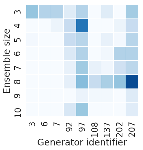
Figure 8. Frequencies of the most used generators.

The smallest size of generators ($s$=3) includes several generators with the smallest identifiers (3, 6, and 7). This is mainly because the IG constructed most of its solutions with these generators, IG iterates through the generators starting from the one with index 0. But it also includes generator number 207.

Focusing on the most used generators for all ensembles, there are three strong generators (that appear in most of the ensemble sizes): generator 92, 97, and 207. These generators probably are able to generate diverse types of MNIST digits.

6.6. Computational Cost

An important advantage of re-purposing the GANs is we get generative models without requiring the computational cost of training the GANs from the beginning to optimize the new objective. Here, we report the average computational time of running the different methods presented here.

The heuristic greedy methods (IG and RG) spent between 2.1 minutes (mins) for $s$=3 and 307.2 mins (when $s$=7). This last high computational cost makes these methods impractical to find ensembles with larger ensembles.

The GA spent 181.2 mins on average to address REO-GEN and 204.8 mins on average to finish when solving NREO-GEN. In the case of the proposed EAs, there is not a correlation between $s$ and the computation time, since the stop condition is performing 10,000 fitness evaluations.

It seems considerable computational cost, but these evolutionary methods are able to return a population of 100 competitive generative models. The average computational cost spent to train each one of the GAN used to create the ensembles is about  60 mins.

It is noticeable that according to the evolution of the fitness shown in Figure 7, both GA proposed here are able to converge to ensembles with high output diversity within the first 5,000 fitness evaluations. Therefore, they could be executed for half of the time and they still could keep returning very competitive results.

Thus, we can see the benefit of applying the proposed methodology and answer to RQ1: Is it possible to re-purpose GANs trained in terms of a given objective (e.g., FID) to optimize another objective (e.g., TVD) without requiring applying the high computational cost of GAN training? is yes. Since the GA re-purposes the generative models requiring a bounded computational time, which is much lower than re-train a number of models to optimize them for the new objective (if it is possible to optimize such a new objective).

7. Conclusions and Future Work

We have empirically shown that EEL can be applied to re-purpose GANs by optimizing the diversity, as measured by TVD, of the generated samples. Specifically, starting from a number of generators previously trained, we defined an optimization problem to combine them in ensembles able to enhance the diversity of the samples generated. We devised two heuristics (greedy), IG and RG, and two different evolutionary approaches to address the problem. The first evolutionary approach addressed REO-GEN, in which the size of the ensemble is specified as a restriction. The second evolutionary approach solved NREO-GEN, which restriction is the maximum size of the ensemble.

These methods were tested on the MNIST. The results demonstrated that both evolutionary approaches construct generative models that greatly improve the diversity of the pre-trained generators while requiring a bounded computational cost. The best TVD results were obtained when the GA was used to address NREO-GEN. The degree of freedom of searching for ensembles without specific sizes allows this method to move through the search space in the way that it converges to better results than the other methods.

Even the greedy methods were the least competitive ones, they also found ensembles that improved diversity. However, they were able to find small ensembles since they become impractical due to the required computational cost when the sizes increased.

When evaluating the quality of the computed ensembles, we have shown that they critically improve the TVD, but they also improve the FID. Additionally, ensembles of size four provided the best results for the problem of generating MNIST digits. Actually, 46.7% of the ensembles returned by the GA that solves NREO-GEN had this specific size.

Future work will include the evaluation of other evolutionary approaches that will encode the weights in a different way such as a larger set of integers or continuous values. We will dive into the predominant generators in the built ensembles to find specific characteristics. In addition, we will address the problem applying a multi-objective approach in order to see the capability of such a methodology in finding ensembles that simultaneously optimize quality (FID) and diversity (TVD). Moreover, we want to evaluate our evolutionary approach with other datasets that require more complex networks (e.g, CIFAR-10, CIFAR-100 or CelebA).

References

- (1)
- Abbass (2003) Hussein A Abbass. 2003. Pareto neuro-evolution: Constructing ensemble of neural networks using multi-objective optimization. In The 2003 Congress on Evolutionary Computation, 2003. CEC’03., Vol. 3. IEEE, 2074–2080.
- Aburomman and Reaz (2016) Abdulla Amin Aburomman and Mamun Bin Ibne Reaz. 2016. A novel SVM-kNN-PSO ensemble method for intrusion detection system. Applied Soft Computing 38 (2016), 360–372.
- Al-Dujaili et al. (2018) Abdullah Al-Dujaili, Tom Schmiedlechner, Erik Hemberg, and Una-May O’Reilly. 2018. Towards distributed coevolutionary GANs. In AAAI 2018 Fall Symposium.
- Al-Sahaf et al. (2019) Harith Al-Sahaf, Ying Bi, Qi Chen, Andrew Lensen, Yi Mei, Yanan Sun, Binh Tran, Bing Xue, and Mengjie Zhang. 2019. A survey on evolutionary machine learning. Journal of the Royal Society of New Zealand 49, 2 (2019), 205–228.
- Alexandropoulos et al. (2019) Stamatios-Aggelos N. Alexandropoulos, Christos K. Aridas, Sotiris B. Kotsiantis, and Michael N. Vrahatis. 2019. Multi-Objective Evolutionary Optimization Algorithms for Machine Learning: A Recent Survey. Springer International Publishing, Cham, 35–55.
- Arjovsky and Bottou (2017) Martin Arjovsky and Léon Bottou. 2017. Towards Principled Methods for Training Generative Adversarial Networks. arXiv e-prints, art. arXiv preprint arXiv:1701.04862 (2017).
- Arora et al. (2018) Sanjeev Arora, Andrej Risteski, and Yi Zhang. 2018. Do GANs learn the distribution? Some Theory and Empirics. In International Conference on Learning Representations. https://openreview.net/forum?id=BJehNfW0-
- Bhowan et al. (2011) Urvesh Bhowan, Mark Johnston, and Mengjie Zhang. 2011. Evolving Ensembles in Multi-Objective Genetic Programming for Classification with Unbalanced Data. In Proceedings of the 13th Annual Conference on Genetic and Evolutionary Computation (GECCO ’11). Association for Computing Machinery, New York, NY, USA, 1331–1338.
- Bi et al. (2019) Ying Bi, Bing Xue, and Mengjie Zhang. 2019. An Automated Ensemble Learning Framework Using Genetic Programming for Image Classification. In Proceedings of the Genetic and Evolutionary Computation Conference (GECCO ’19). Association for Computing Machinery, New York, NY, USA, 365–373. https://doi.org/10.1145/3321707.3321750
- Borji (2019) Ali Borji. 2019. Pros and cons of gan evaluation measures. Computer Vision and Image Understanding 179 (2019), 41–65.
- Chandra and Yao (2006) Arjun Chandra and Xin Yao. 2006. Ensemble learning using multi-objective evolutionary algorithms. Journal of Mathematical Modelling and Algorithms 5, 4 (2006), 417–445.
- Chen et al. (2019) Y. Chen, Y. Yang, W. Wang, and C. . J. Kuo. 2019. Ensembles of Feedforward-Designed Convolutional Neural Networks. In 2019 IEEE International Conference on Image Processing (ICIP). 3796–3800.
- Chintala et al. (2016) Soumith Chintala, Emily Denton, Martin Arjovsky, and Michael Mathieu. 2016. How to Train a GAN? Tips and tricks to make GANs work. https://github.com/soumith/ganhacks. (2016).
- Dick et al. (2018) Grant Dick, Caitlin A Owen, and Peter A Whigham. 2018. Evolving bagging ensembles using a spatially-structured niching method. In Proceedings of the Genetic and Evolutionary Computation Conference. 418–425.
- Dietterich (2000) Thomas G. Dietterich. 2000. Ensemble Methods in Machine Learning. In Multiple Classifier Systems. Springer Berlin Heidelberg, Berlin, Heidelberg, 1–15.
- Durugkar et al. (2016) Ishan Durugkar, Ian Gemp, and Sridhar Mahadevan. 2016. Generative multi-adversarial networks. arXiv preprint arXiv:1611.01673 (2016).
- Fernandes et al. (2019) E. Fernandes, A. C. P. d. L. F. De Carvalho, and X. Yao. 2019. Ensemble of Classifiers based on MultiObjective Genetic Sampling for Imbalanced Data. IEEE Transactions on Knowledge and Data Engineering (2019), 1–1. https://doi.org/10.1109/TKDE.2019.2898861
- Fitzgerald et al. (2013) Jeannie Fitzgerald, R Muhammad Atif Azad, and Conor Ryan. 2013. A bootstrapping approach to reduce over-fitting in genetic programming. In Proceedings of the 15th annual conference companion on Genetic and evolutionary computation. 1113–1120.
- Folino et al. (2003) Gianluigi Folino, Clara Pizzuti, and Giandomenico Spezzano. 2003. Ensemble techniques for parallel genetic programming based classifiers. In European Conference on Genetic Programming. Springer, 59–69.
- Folino et al. (2006) Gianluigi Folino, Clara Pizzuti, and Giandomenico Spezzano. 2006. GP ensembles for large-scale data classification. IEEE Transactions on Evolutionary Computation 10, 5 (2006), 604–616.
- Gama and Brazdil (2000) João Gama and Pavel Brazdil. 2000. Cascade generalization. Machine learning 41, 3 (2000), 315–343.
- Goodfellow et al. (2014) Ian Goodfellow, Jean Pouget-Abadie, Mehdi Mirza, Bing Xu, David Warde-Farley, Sherjil Ozair, Aaron Courville, and Yoshua Bengio. 2014. Generative adversarial nets. In Advances in neural information processing systems. 2672–2680.
- Grover and Ermon (2018) Aditya Grover and Stefano Ermon. 2018. Boosted generative models. In Thirty-Second AAAI Conference on Artificial Intelligence.
- Gulrajani et al. (2017) Ishaan Gulrajani, Faruk Ahmed, Martin Arjovsky, Vincent Dumoulin, and Aaron C Courville. 2017. Improved training of wasserstein gans. In Advances in neural information processing systems. 5767–5777.
- Heusel et al. (2017) Martin Heusel, Hubert Ramsauer, Thomas Unterthiner, and Bernhard Nessler. 2017. GANs Trained by a Two Time-Scale Update Rule Converge to a Local Nash Equilibrium. arXiv preprint arXiv:1706.08500 (2017).
- Hoang et al. (2017) Quan Hoang, Tu Dinh Nguyen, Trung Le, and Dinh Phung. 2017. Multi-generator generative adversarial nets. arXiv preprint arXiv:1708.02556 (2017).
- Iba (1999) Hitoshi Iba. 1999. Bagging, boosting, and bloating in genetic programming. In Proceedings of the 1st Annual Conference on Genetic and Evolutionary Computation-Volume 2. 1053–1060.
- Islam et al. (2003) Md M Islam, Xin Yao, and Kazuyuki Murase. 2003. A constructive algorithm for training cooperative neural network ensembles. IEEE Transactions on neural networks 14, 4 (2003), 820–834.
- Jin (2006) Yaochu Jin. 2006. Multi-objective machine learning. Vol. 16. Springer Science & Business Media.
- Kim and Yoo (2019) Jinhan Kim and Shin Yoo. 2019. Software review: DEAP (Distributed Evolutionary Algorithm in Python) library. Genetic Programming and Evolvable Machines 20, 1 (2019), 139–142.
- Krizhevsky et al. (2012) Alex Krizhevsky, Ilya Sutskever, and Geoffrey E Hinton. 2012. Imagenet classification with deep convolutional neural networks. In Advances in neural information processing systems. 1097–1105.
- Langdon et al. (2002) William B Langdon, SJ Barrett, and Bernard F Buxton. 2002. Combining decision trees and neural networks for drug discovery. In European Conference on Genetic Programming. Springer, 60–70.
- Larcher and Barbosa (2019) Celio H. N. Larcher and Helio J. C. Barbosa. 2019. Auto-CVE: A Coevolutionary Approach to Evolve Ensembles in Automated Machine Learning. In Proceedings of the Genetic and Evolutionary Computation Conference (GECCO ’19). Association for Computing Machinery, New York, NY, USA, 392–400. https://doi.org/10.1145/3321707.3321844
- LeCun (1998) Yann LeCun. 1998. The MNIST database of handwritten digits. http://yann. lecun. com/exdb/mnist/ (1998).
- Li et al. (2017) Chengtao Li, David Alvarez-Melis, Keyulu Xu, Stefanie Jegelka, and Suvrit Sra. 2017. Distributional Adversarial Networks. arXiv preprint arXiv:1706.09549 (2017).
- Lima et al. (2013) Aranildo R Lima, Alex J Cannon, and William W Hsieh. 2013. Nonlinear regression in environmental sciences by support vector machines combined with evolutionary strategy. Computers & Geosciences 50 (2013), 136–144.
- Liu et al. (2000) Yong Liu, Xin Yao, and Tetsuya Higuchi. 2000. Evolutionary ensembles with negative correlation learning. IEEE Transactions on Evolutionary Computation 4, 4 (2000), 380–387.
- Loshchilov (2013) Ilya Loshchilov. 2013. Surrogate-assisted evolutionary algorithms. Ph.D. Dissertation. University Paris South Paris XI; National Institute for Research in Computer Science and Automatic-INRIA.
- Mao et al. (2017) Xudong Mao, Qing Li, Haoran Xie, Raymond YK Lau, Zhen Wang, and Stephen Paul Smolley. 2017. Least squares generative adversarial networks. In Proceedings of the IEEE International Conference on Computer Vision. 2794–2802.
- Mauša and Grbac (2017) Goran Mauša and Tihana Galinac Grbac. 2017. Co-evolutionary multi-population genetic programming for classification in software defect prediction: an empirical case study. Applied soft computing 55 (2017), 331–351.
- Meng and Xu (2018) QN Meng and Xun Xu. 2018. Price forecasting using an ACO-based support vector regression ensemble in cloud manufacturing. Computers & Industrial Engineering 125 (2018), 171–177.
- Nguyen et al. (2017) Tu Nguyen, Trung Le, Hung Vu, and Dinh Phung. 2017. Dual discriminator generative adversarial nets. In Advances in Neural Information Processing Systems. 2670–2680.
- Padilha et al. (2016) Carlos Alberto de Araújo Padilha, Dante Augusto Couto Barone, and Adrião Duarte Dória Neto. 2016. A Multi-Level Approach Using Genetic Algorithms in an Ensemble of Least Squares Support Vector Machines. Know.-Based Syst. 106, C (2016), 85–95.
- Pan et al. (2019) Zhaoqing Pan, Weijie Yu, Xiaokai Yi, Asifullah Khan, Feng Yuan, and Yuhui Zheng. 2019. Recent progress on generative adversarial networks (GANs): A survey. IEEE Access 7 (2019), 36322–36333.
- Pławiak et al. (2019) Paweł Pławiak, Moloud Abdar, and U Rajendra Acharya. 2019. Application of new deep genetic cascade ensemble of SVM classifiers to predict the Australian credit scoring. Applied Soft Computing 84 (2019), 105740.
- Pulido et al. (2016) Martha Pulido, Patricia Melin, and Oscar Castillo. 2016. Design of Ensemble Neural Networks for Predicting the US Dollar/MX Time Series with Particle Swarm Optimization. In Recent Developments and New Direction in Soft-Computing Foundations and Applications. Springer, 317–329.
- Radford et al. (2015) Alec Radford, Luke Metz, and Soumith Chintala. 2015. Unsupervised Representation Learning with Deep Convolutional Generative Adversarial Networks. arXiv preprint arXiv:1511.06434 (2015).
- Ribeiro and Reynoso-Meza (2018) Victor Henrique Alves Ribeiro and Gilberto Reynoso-Meza. 2018. A multi-objective optimization design framework for ensemble generation. In Proceedings of the Genetic and Evolutionary Computation Conference Companion. 1882–1885.
- Ripon et al. (2020) Shamim Ripon, Md Golam Sarowar, Fahima Qasim, and Shamse Tasnim Cynthia. 2020. An Efficient Classification of Tuberous Sclerosis Disease Using Nature Inspired PSO and ACO Based Optimized Neural Network. In Nature Inspired Computing for Data Science. Springer, 1–28.
- Sajjadi et al. (2018) Mehdi SM Sajjadi, Olivier Bachem, Mario Lucic, Olivier Bousquet, and Sylvain Gelly. 2018. Assessing generative models via precision and recall. In Advances in Neural Information Processing Systems. 5228–5237.
- Salimans et al. (2016) Tim Salimans, Ian Goodfellow, Wojciech Zaremba, Vicki Cheung, Alec Radford, and Xi Chen. 2016. Improved techniques for training gans. In Advances in neural information processing systems. 2234–2242.
- Schapire (1990) Robert E Schapire. 1990. The strength of weak learnability. Machine learning 5, 2 (1990), 197–227.
- Schmiedlechner et al. (2018) Tom Schmiedlechner, Ignavier Ng Zhi Yong, Abdullah Al-Dujaili, Erik Hemberg, and Una-May O’Reilly. 2018. Lipizzaner: A System That Scales Robust Generative Adversarial Network Training. In the 32nd Conference on Neural Information Processing Systems (NeurIPS 2018) Workshop on Systems for ML and Open Source Software.
- Sohn and Yoo (2019) Jeongju Sohn and Shin Yoo. 2019. Why Train-and-Select When You Can Use Them All? Ensemble Model for Fault Localisation. In Proceedings of the Genetic and Evolutionary Computation Conference (GECCO ’19). Association for Computing Machinery, New York, NY, USA, 1408–1416. https://doi.org/10.1145/3321707.3321873
- Tolstikhin et al. (2017) Ilya O Tolstikhin, Sylvain Gelly, Olivier Bousquet, Carl-Johann Simon-Gabriel, and Bernhard Schölkopf. 2017. AdaGAN: Boosting generative models. In Advances in Neural Information Processing Systems. 5424–5433.
- Toutouh et al. (2019) Jamal Toutouh, Erik Hemberg, and Una-May O’Reilly. 2019. Spatial Evolutionary Generative Adversarial Networks. In Proceedings of the Genetic and Evolutionary Computation Conference (GECCO ’19). ACM, New York, NY, USA, 472–480. https://doi.org/10.1145/3321707.3321860
- Tran et al. (2018) Cao Truong Tran, Mengjie Zhang, Bing Xue, and Peter Andreae. 2018. Genetic Programming with Interval Functions and Ensemble Learning for Classification with Incomplete Data. In Australasian Joint Conference on Artificial Intelligence. Springer, 577–589.
- Wang et al. (2016) Yaxing Wang, Lichao Zhang, and Joost van de Weijer. 2016. Ensembles of generative adversarial networks. arXiv preprint arXiv:1612.00991 (2016).
- Wang et al. (2019) Zhengwei Wang, Qi She, and Tomas E Ward. 2019. Generative adversarial networks: A survey and taxonomy. arXiv preprint arXiv:1906.01529 (2019).
- Wolpert (1992) David H Wolpert. 1992. Stacked generalization. Neural networks 5, 2 (1992), 241–259.
- Wu et al. (2017) Xian Wu, Kun Xu, and Peter Hall. 2017. A survey of image synthesis and editing with generative adversarial networks. Tsinghua Science and Technology 22, 6 (2017), 660–674.
- Zhang et al. (2017) C. Zhang, P. Lim, A. K. Qin, and K. C. Tan. 2017. Multiobjective Deep Belief Networks Ensemble for Remaining Useful Life Estimation in Prognostics. IEEE Transactions on Neural Networks and Learning Systems 28, 10 (Oct 2017), 2306–2318. https://doi.org/10.1109/TNNLS.2016.2582798
- Zhang and Ma (2012) Cha Zhang and Yunqian Ma. 2012. Ensemble machine learning: methods and applications. Springer.
- Zhou et al. (2002) Zhi-Hua Zhou, Jianxin Wu, and Wei Tang. 2002. Ensembling neural networks: many could be better than all. Artificial intelligence 137, 1-2 (2002), 239–263.