Bounding the expectation of the supremum of empirical processes indexed by Hölder classes

Abstract

In this note, we provide upper bounds on the expectation of the supremum of empirical processes indexed by Hölder classes of any smoothness and for any distribution supported on a bounded set in $\mathbb{R}^{d}$. These results can alternatively be seen as non-asymptotic risk bounds, when the unknown distribution is estimated by its empirical counterpart, based on $n$ independent observations, and the error of estimation is quantified by integral probability metrics (IPM). In particular, IPM indexed by Hölder classes are considered and the corresponding rates are derived. These results interpolate between two well-known extreme cases: the rate $n^{-1/d}$ corresponding to the Wassertein-1 distance (the least smooth case) and the fast rate $n^{-1/2}$ corresponding to very smooth functions (for instance, functions from a RKHS defined by a bounded kernel).

1 Introduction

In many problems of mathematical statistics and learning theory, a crucial step is to understand how well the empirical distribution of a sample approximates the underlying true distribution. The theory of empirical processes is devoted to this question. There are many papers and books treating this and related problems, both from asymptotic and nonasymptotic points of view; see, for instance, van der Vaart and Wellner, (1996); del Barrio et al., (2007). Among many remarkable achievements of the theory of empirical processes, there are two results that have been particularly often evoked and used in the recent literature in statistics and machine learning.

To quickly present these two results, let us give some details on the framework. It is assumed that $n$ independent copies $X_{1},\ldots,X_{n}$ of a random variable $X$ taking its values in the $d$-dimensional hypercube $[0,1]^{d}$ are observed. The aforementioned two results characterize the order of magnitude of supremum of the empirical process $\mathbb{X}_{n}(f)=\frac{1}{n}\sum_{i=1}f(X_{i})-\mathbb{E}[f(X)]$ over some class of functions $\mathcal{F}$. More precisely, the first result established by Dudley, (1968) states that $\sup_{f\in\sf Lip(1)}\mathbb{X}_{n}(f)$ is of order $O(n^{-1/d})$,where ${\sf Lip(1)}$ is the set of all the Lipschitz-continuous functions with Lipschitz constant 1. The second result (Briol et al.,, 2019, Lemma 1), tells us that if $\mathcal{F}$ contains functions that are smooth enough, for instance functions that are in a finite ball of a RKHS defined by a bounded kernel, then $\sup_{f\in\mathcal{F}}\mathbb{X}_{n}(f)$ is of order $O(n^{-1/2})$, i.e., the same order as in the case when $\mathcal{F}$ contains only one function.

The main result of this note provides an interpolation between the two aforementioned results. Roughly speaking, it shows that if $\mathcal{F}$ is the class of functions defined on $[0,1]^{d}$ that are Hölder-continuous for a given constant $L$ and a given order $\alpha>0$, then the supremum of the empirical process over $\mathcal{F}$ is of order $O(n^{-(\frac{\alpha}{d}\wedge\frac{1}{2})})$ with an additional slowly varying factor $\log n$ when $\alpha=d/2$. Clearly, when $\alpha=1$ this coincides with the result from Dudley, (1968), while for $\alpha\geq d/2$ we get the fast and dimension-free rate $n^{-1/2}$, up to a log factor.

The rest of this note is organized as follows. We complete this introduction by providing all the important notations used throughout this note. Section 2 is devoted to presenting and formally defining Hölder classes and Integral Probability Metrics (IPM). In Section 3, we expose some important concepts and results from empirical process theory needed for our proofs. We end this note by stating our main theorem in Section 4. Some extensions are mentioned in Section 5. The proofs are postponed to the appendix.

Notations

A multi-index $\boldsymbol{k}$ is a vector with integer coordinates $(k_{1},\dots,k_{d})$. We write $\lvert\boldsymbol{k}\rvert=\sum_{i=1}^{d}k_{i}$. For a given multi-index $\boldsymbol{k}=(k_{1},\dots,k_{d})$, we define the differential operator

$$D^{\boldsymbol{k}}=\frac{\partial^{\rvert\boldsymbol{k}\lvert}}{\partial x_{1}^{k_{1}}\dots\partial x_{d}^{k_{d}}}.$$ (1)

For any positive real number $x$, $\lfloor x\rfloor$ denotes the largest integer strictly smaller than $x$. We let $\mathcal{X}$ be a convex bounded set in $\mathbb{R}^{d}$ with non-empty interior. We assume that all the functions and function classes considered in this note are supported on the bounded set $\mathcal{X}$. For any integer $k$, we denote by $C^{k}(\mathcal{X},\mathbb{R})$ the class of real-valued functions with domain $\mathcal{X}$ which are $k$-times differentiable with continuous $k$-th differentials. For any real-valued bounded function $f$ on $\mathcal{X}$, we let $\lVert f\rVert_{\infty}\coloneqq\sup_{x\in\mathcal{X}}\lvert f(x)\rvert\in[0,+\infty)$. Note that we can consider the essential supremum instead of the supremum over $\mathcal{X}$ in which case our results would hold almost surely. We let $\lVert\cdot\rVert$ denote some norm on $\mathbb{R}^{d}$. We denote by $\sigma_{1},\dots,\sigma_{n}$ i.i.d. Rademacher random variables, i.e., discrete random variables such that $\mathbb{P}(\sigma_{1}=1)=\mathbb{P}(\sigma_{1}=-1)=1/2$ which are independent of any other source of randomness. We use the convention $\nicefrac{{1}}{{0}}=+\infty$.

2 A primer on Hölder classes and integral probability metrics

In this section we define Hölder classes of functions and integral probability metrics. We then discuss some properties of these notions and highlight their role in statistics and statistical learning theory.

2.1 Hölder classes

A central problem in nonparametric statistics is to estimate a function belonging to an infinite-dimensional space (e.g., density estimation, regression function estimation, hazard function estimation), see Tsybakov, (2008) for an introduction to the topic of nonparametric estimation. To obtain nontrivial rates of convergence, some kind of regularity is assumed on the function of interest. It can be expressed as conditions on the function itself, on its derivatives, on the coefficients of the function in a given basis, etc. Hölder classes are one of the most common classes considered in the nonparametric estimation literature, they form a natural extension of Lipschitz-continuous functions and can be formalised with the following simple conditions. For any real number $\alpha>0$, we define the Hölder norm of smoothness $\alpha$ of a $\lfloor\alpha\rfloor$-times differentiable function $f$ as

$$\lVert f\rVert_{\mathcal{H}^{\alpha}}\coloneqq\max_{\lvert k\rvert\leq\lfloor\alpha\rfloor}\lVert D^{k}f\rVert_{\infty}+\max_{\lvert k\rvert=\lfloor\alpha\rfloor}\sup_{x\neq y}\frac{\lvert D^{k}f(x)-D^{k}f(y)\rvert}{\lVert x-y\rVert^{\alpha-\lfloor\alpha\rfloor}}.$$ (2)

The Hölder ball of smoothness $\alpha$ and radius $L>0$, denoted by $\mathcal{H}^{\alpha}(L)$, is then defined as the class of $\lfloor\alpha\rfloor$-times continuously differentiable functions with Hölder norm bounded by the radius $L$:

$$\mathcal{\mathcal{H}}^{\alpha}(L)=\left\{f\in C^{\lfloor\alpha\rfloor}(\mathcal{X},\mathbb{R})\mid\lVert f\rVert_{\mathcal{H}^{\alpha}}\leq L\right\}.$$ (3)

To get a grasp of why Hölder classes are convenient, let us consider the case $d=1$. In this setting, one can easily derive an upper bound on the remainder of the best polynomial approximation of any given Hölder function. Indeed, for any positive $\alpha>0$ with $\lfloor\alpha\rfloor=\ell$, for any function $f\in\mathcal{H}^{\alpha}(L)$, Taylor’s theorem yields that for any points $x,y\in\mathcal{X}$,

$$\bigg{\lvert}f(y)-\sum_{k=0}^{\ell}\frac{f^{(k)}(x)}{k!}(y-x)^{k}\bigg{\rvert} \leq\frac{\lvert y-x\rvert^{\ell}}{(\ell-1)!}\int_{0}^{1}\lvert f^{(\ell)}(x+t(y-x))-f^{(\ell)}(x)\rvert(1-t)^{\ell}dt$$ (4)

$$\leq L\frac{\lvert y-x\rvert^{\alpha}}{(\ell-1)!}\int_{0}^{1}t^{\alpha-\ell}(1-t)^{\ell}dt$$ (5)

$$\leq L\frac{\lvert y-x\rvert^{\alpha}}{\ell!}.$$ (6)

Note that this bound holds uniformly over the Hölder ball $\mathcal{H}^{\alpha}(L)$.

2.2 Integral probability metrics

The class $\mathcal{H}^{1}$(1) of $1$-Lipschitz functions has received a lot of attention in the optimal transport literature; see (Santambrogio,, 2015) for an overview of the topic of mathematical optimal transport. This interest comes from the Kantorovitch duality, which implies that the Wasserstein-1 distance (also known as the earth mover’s distance) can be expressed, for any probability measures $P,Q$, as a supremum of some functional over $1$-Lipschitz functions:

$$W_{1}(P,Q)=\sup_{f\in\mathcal{H}^{1}(1)}\lvert\mathbb{E}_{X\sim P}f(X)-\mathbb{E}_{Y\sim Q}f(Y)\rvert.$$ (7)

More generally, for a given class $\mathcal{F}$ of bounded functions, one can define a pseudo-metric on the space of probability measures, the integral probability metric (IPM) induced by the class $\mathcal{F}$, as

$$d_{\mathcal{F}}(P,Q)=\sup_{f\in\mathcal{F}}\lvert\mathbb{E}_{X\sim P}f(X)-\mathbb{E}_{Y\sim Q}f(Y)\rvert.$$ (8)

The literature on IPM has recently been boosted by the advent of adversarial generative models (Arjovsky et al.,, 2017; Goodfellow et al.,, 2014). A reason for this is that an IPM can be seen as an adversarial loss: to compare two probability distributions, it seeks for the function which discriminates the most the two distributions in expectation. Initially studied by the deep learning community, impressive empirical results obtained by adversarial generative models on several tasks such as image generation led statisticians to study it theoretically (Liang,, 2018; Chen et al.,, 2020; Briol et al.,, 2019) (see also Sriperumbudur et al., (2012) for statistical results on IPM in a general framework). Since, as pointed out earlier, Lipschitz functions are also Hölder, one can wonder what happens for IPM indexed by general Hölder classes. Such IPM already appeared in the literature: Scetbon et al., (2020) showed that $\alpha$-Hölder IPM with smoothness $\alpha\leq 1$ correspond to the cost of a generalized optimal transport problem.

To further motivate our study, let us consider the abstract problem of minimum distance estimation: for a given probability measure $P$, find a distribution $Q$ in a given set of probability measures $\mathcal{Q}$ such that $Q$ is close to $P$ under the metric $d_{\mathcal{F}}$:

$$\min_{Q\in\mathcal{Q}}d_{\mathcal{F}}(Q,P).$$ (9)

For example, when $\mathcal{F}$ is taken to be the class of $1$-Lipschitz function, this problem is known as minimum Kantorovitch estimation (Bassetti et al.,, 2006). In statistics, the probability $P$ is usually unknown and one is only given i.i.d. samples $X_{1},\dots,X_{n}$ from the probability distribution $P$. A natural strategy is then to employ the empirical distribution $P_{n}=1/n\sum_{i=1}^{n}\delta_{X_{i}}$ as a proxy for the theoretical distribution and instead of (9) solve the problem:

$$\min_{Q\in\mathcal{Q}}d_{\mathcal{F}}(Q,P_{n}).$$ (10)

Since the triangle inequality yields

$$\lvert d_{\mathcal{F}}(Q,P)-d_{\mathcal{F}}(Q,P_{n})\rvert\leq d_{\mathcal{F}}(P,P_{n})=\sup_{f\in\mathcal{F}}\bigg{\lvert}\frac{1}{n}\sum_{i=1}^{n}f(X_{i})-\mathbb{E}f(X)\bigg{\rvert},$$ (11)

one question of interest is to measure how fast the empirical measure approximates the true measure under the IPM $d_{\mathcal{F}}$. If the rates are fast, we do not loose much by considering the empirical problem (10) instead of the theoretical one of (9). However if the rates are slow, one cannot expect the distances of the solutions to the measure $P$ to be close. We will see in the next section that the latter expression corresponds to the supremum of the empirical process indexed by the class $\mathcal{F}$, it will enable us to leverage the rich literature on empirical processes to obtain rates of convergence for $d_{\mathcal{F}}(P,P_{n})$.

3 Empirical processes, metric entropy and Dudley’s bounds

This section provides a short account of the notions and tools from the theory of empirical processes which are necessary for stating and establishing the main result.

3.1 Empirical processes

Empirical process are ubiquitous in statistical learning theory, we refer the reader to Koltchinskii, (2011); Giné and Nickl, (2016) for a general presentation of results on empirical processes and their link with statistics and learning theory. For clarity, we begin by recalling the definition of an empirical process.

Definition 1.

Let $\mathcal{F}$ be a class of real-valued functions $f\colon\mathcal{X}\to\mathbb{R}$, where $(\mathcal{X},\mathcal{A},P)$ is a probability space. Let $X$ be a random point in $\mathcal{X}$ distributed according to the distribution $P$ and let $X_{1},\dots,X_{n}$ be independent copies of $X$. The random process $\big{(}\mathbb{X}_{n}(f)\big{)}_{f\in\mathcal{F}}$ defined by

$$\mathbb{X}_{n}(f)\coloneqq\frac{1}{n}\sum_{i=1}^{n}f(X_{i})-\mathbb{E}f(X)$$ (12)

is called an empirical process indexed by $\mathcal{F}$.

In our case, we are interested in controlling the (expectation of the) supremum of an empirical process, a common case in the literature. Most of the time, the first step to apply for achieving this goal is to “symmetrize” the empirical process as allowed by the following lemma. Let $\widehat{R}_{n}(\mathcal{F})$ be the empirical Rademacher complexity of function class $\mathcal{F}$, defined as

$$\widehat{R}_{n}(\mathcal{F})=\mathbb{E}\left[\sup_{f\in\mathcal{F}}\frac{1}{n}\sum_{i=1}^{n}\sigma_{i}f(X_{i})\,\Big{|}\,X_{1},\ldots,X_{n}\right].$$ (13)

Lemma 1 (Symmetrization).

For any class $\mathcal{F}$ of $P$-integrable functions,

$$\mathbb{E}\bigg{[}\sup_{f\in\mathcal{F}}\lvert\mathbb{X}_{n}(f)\rvert\bigg{]}\leq 2\,\mathbb{E}\big{[}\widehat{R}_{n}(\mathcal{F})\big{]}.$$ (14)

The advantage of Rademacher processes is that, regardless of the distribution of the random variable $X$ and the function class $\mathcal{F}$, for a fixed sample $X_{1},\dots,X_{n}$, the random variable $\sum_{i=1}^{n}\sigma_{i}f(X_{i})$ has a sub-Gaussian behavior, in the following sense.

Definition 2 (Sub-Gaussian behavior).

A centered random variable $Y$ has a sub-Gaussian behavior if there exists a positive constant $\sigma$ such that

$$\mathbb{E}e^{\lambda Y}\leq e^{\lambda^{2}\sigma^{2}/2},\quad\forall\lambda\in\mathbb{R}.$$ (15)

In that case, we define the sub-Gaussian norm of $Y$ as

$$\lVert Y\rVert_{\psi_{2}}=\inf\left\{t>0:\mathbb{E}e^{Y^{2}/t^{2}}\leq 2\right\}.$$ (16)

Having a sub-Gaussian behavior essentially means to be at least as concentrated as a Gaussian random variable around its mean. Our definition is equivalent to the tail inequalities

$$\mathbb{P}(\lvert Y\rvert>t)\leq 2e^{-t^{2}/(2\sigma^{2})},\quad\forall t>0.$$ (17)

This type of behavior will be crucial to obtain the main result of this note. Indeed, as we will see, the behavior of the supremum of an empirical process (and more generally a stochastic process) which has sub-Gaussian increments exclusively depends on the topology of the space by which the process is indexed.

3.2 Metric entropy

Let $(T,d)$ be a totally bounded metric space, i.e., for every real number $\varepsilon>0$, there exists a finite collection of open balls of radius $\varepsilon$ whose union contains $T$. We give a formal definition of such finite collections, see also Figure 1 for an illustration.

Definition 3.

Given $\varepsilon>0$, a subset $T_{\varepsilon}\subset T$ is called an $\varepsilon$-cover of $T$ if for every $t\in T$, there exists $s\in T_{\varepsilon}$ such that $d(s,t)\leq\varepsilon$.

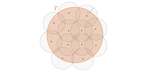
Figure 1: Illustration of an $\varepsilon$-cover for some space $T$.

Note that adding any point to an $\varepsilon$-cover still yields an $\varepsilon$-cover. Thus we can look for $\varepsilon$-covers of a set with smallest cardinality, which we call covering number.

Definition 4.

The $\varepsilon$-covering number of $T$, denoted by $\mathcal{N}(T,d,\varepsilon)$, is the cardinality of the smallest $\varepsilon$-cover of $T$, that is

$$\mathcal{N}(T,d,\varepsilon)\coloneqq\min\big{\{}\lvert T_{\varepsilon}\rvert:T_{\varepsilon}\text{ is an }\varepsilon\text{-cover of }T\big{\}}.$$ (18)

The metric entropy of $T$ is given by the logarithm of the $\varepsilon$-covering number.

Remark 1.

A totally bounded metric space $(T,d)$ is pre-compact in the sense that its closure is compact. The metric entropy (or entropic numbers) of $(T,d)$ can then be seen as some measure of compactness of the space. Indeed, $\mathcal{N}(T,d,\varepsilon)$ quantifies precisely how many balls of radius $\varepsilon$ are needed to cover the whole space $T$.

Entropic numbers for Hölder classes are known and can be found in e.g. Shiryayev, (1993); van der Vaart and Wellner, (1996).

Theorem 1 (Theorem 2.7.3 in van der Vaart and Wellner, (1996)).

Let $\mathcal{X}$ be a bounded, convex subset of $\mathbb{R}^{d}$ with nonempty interior. There exists a constant $K_{\alpha,d}$ depending only on $\alpha$ and $d$ such that, for every $\varepsilon>0$,

$$\log\mathcal{N}(\mathcal{H}^{\alpha}(1),\lVert\cdot\rVert_{\infty},\varepsilon)\leq K_{\alpha,d}\lambda_{d}(\mathcal{X}^{1})\,\varepsilon^{-d/\alpha},$$ (19)

where $\lambda_{d}$ is the $d$-dimensional Lebesgue measure and $\mathcal{X}^{1}$ is the $1$-blowup of $\mathcal{X}$: $\mathcal{X}^{1}=\{y:\inf_{x\in\mathcal{X}}\lVert y-x\rVert<1\}$.

3.3 Dudley’s bound and its refined version

We now present classic results which show the link between the topology of the indexing set and the behavior of the supremum of the corresponding empirical process. Following (Vershynin,, 2018, Definition 8.1.1), for $K\geq 0$, we say that a random process $(X_{t})_{t\in T}$ on a metric space $(T,d)$ has $K$-sub-Gaussian increments if

$$\lVert X_{t}-X_{s}\rVert_{\psi_{2}}\leq Kd(t,s),\quad\text{ for all }\quad t,s\in T.$$ (20)

Theorem 2 (Dudley’s inequality).

Let $(X_{t})_{t\in T}$ be a mean-zero random process on a metric space $(T,d)$ with $K$-sub-Gaussian increments. Then

$$\mathbb{E}\Big{[}\sup_{t\in T}X_{t}\Big{]}\leq CK\int_{0}^{+\infty}\sqrt{\log\mathcal{N}(T,d,\varepsilon)}\,d\varepsilon,$$ (21)

for some universal constant $C>0$.

One drawback of Dudley’s bound is that the integral on the right hand side may diverge if the metric entropy of $T$ tends to infinity at a very fast rate when $\varepsilon\to 0$. For example, when the metric entropy is upper bounded by $\varepsilon^{-\gamma}$, as it was seen to be the case with $\gamma=d/\alpha$ for $\alpha$-Hölder-smooth $d$-variate functions, the integral converges if and only if $\gamma<2$.

An improvement of Dudley’s bound in the case where the process $X_{t}$ is a Rademacher average indexed by a class of functions $\mathcal{F}$—circumventing the problem of divergence of the integral—was proposed by (Srebro et al.,, 2010, Lemma A.3) (see also Srebro and Sridharan, (2010)). Before stating the theorem, let us recall the definition of the $L_{2}(P_{n})$ norm of a function $f$:

$$\lVert f\rVert_{L_{2}(P_{n})}^{2}=\int_{\mathcal{X}}f^{2}\,dP_{n}=\frac{1}{n}\sum_{i=1}^{n}f(X_{i})^{2}.$$ (22)

Theorem 3.

Let $\mathcal{F}\subset\{f\colon\mathcal{X}\to\mathbb{R}\}$ be any class of measurable functions containing the uniformly zero function and let $S_{n}(\mathcal{F})=\sup_{f\in\mathcal{F}}\lVert f\rVert_{L_{2}(P_{n})}$. We have

$$\widehat{R}_{n}(\mathcal{F})\leq\inf_{\tau>0}\left\{4\tau+\frac{12}{\sqrt{n}}\int_{\tau}^{S_{n}(\mathcal{F})}\sqrt{\log\mathcal{N}(\mathcal{F},L_{2}(P_{n}),\varepsilon)}\,d\varepsilon\right\}.$$ (23)

Note that the refined Dudley bound gives an upper bound on the empirical Rademacher process and depends on the metric entropy with respect to the empirical norm $L_{2}(P_{n})$. The following simple lemma shows that the $L_{2}(P_{n})$-norm can be replaced by the supremum-norm in the refined Dudley bound.

Lemma 2.

Let $\mathcal{F}$ be any class of bounded functions defined on $\mathcal{X}$. For any sample $X_{1},\dots,X_{n}$, let $\mathcal{F}_{|X_{1},\ldots,X_{n}}$ be the subset of $\mathbb{R}^{n}$ defined by

$$\mathcal{F}_{|X_{1},\ldots,X_{n}}=\big{\{}u\in\mathbb{R}^{n}:\exists f\in\mathcal{F}\text{ such that }u_{i}=f(X_{i})\text{ for all }i=1,\ldots,n\big{\}}.$$

For any $\varepsilon>0$, we have

$$\mathcal{N}(\mathcal{F},L_{2}(P_{n}),\varepsilon)\leq\mathcal{N}(\mathcal{F}_{|X_{1},\dots,X_{n}},\lVert\cdot\rVert_{\infty},\varepsilon)\leq\mathcal{N}(\mathcal{F},\lVert\cdot\rVert_{\infty},\varepsilon).$$ (24)

Proof.

Let $\{u_{1},\dots,u_{M}\}$ be a minimal $\varepsilon$-net for $\mathcal{F}_{|X_{1},\dots,X_{n}}$ with respect to the supremum norm. Let $f_{1},\ldots,f_{M}\in\mathcal{F}$ be such that $\big{(}f_{j}(X_{1}),\ldots,f_{j}(X_{n}))=u_{j}$ for every $j=1,\ldots,M$. Then, for any $f\in\mathcal{F}$, there exists an index $j\in[M]$ such that $\max_{i}\lvert f(X_{i})-(u_{j})_{i}\rvert=\max_{i}\lvert f(X_{i})-f_{j}(X_{i})\rvert\leq\varepsilon$. Since for any function $f$ in $\mathcal{F}$,

$$\lVert f-f_{j}\rVert_{L_{2}(P_{n})}^{2}=\frac{1}{n}\sum_{i=1}^{n}(f(X_{i})-f_{j}(X_{i}))^{2}\leq\lVert f-f_{j}\rVert_{\infty}^{2},$$ (25)

$\{f_{1},\dots,f_{M}\}$ is an $\varepsilon$-net for $\mathcal{F}$ with respect to the empirical $L_{2}$ norm. This proves the first inequality. Let now $f_{1},\ldots,f_{M}$ be an $\varepsilon$-net of $(\mathcal{F},\lVert\cdot\rVert_{\infty})$. One readily checks that $u_{1},\ldots,u_{M}$ defined by $u_{j}=(f_{j}(X_{1}),\ldots,f_{j}(X_{n}))$ is an $\varepsilon$-net of $\mathcal{F}_{|X_{1},\dots,X_{n}}$. This completes the proof. ∎

4 Main result

We are now in a position to state the main theorem which gives, for an IPM defined by a Hölder class, the rate of convergence of the empirical measure towards its theoretical counterpart.

Theorem 4.

Let $\mathcal{X}\subset\mathbb{R}^{d}$ be a convex bounded set with non-empty interior. Let $\mathcal{H}^{\alpha}(L)$ be the Hölder class of $\alpha$-smooth functions supported on the set $\mathcal{X}$ and with Hölder norm bounded by $L$. For any probability distribution $P$ supported on $\mathcal{X}$, denoting by $P_{n}$ the empirical measure associated to i.i.d. samples $X_{1},\dots,X_{n}\sim P$, we have,

$$\mathbb{E}\big{[}d_{\mathcal{H}^{\alpha}(L)}(P_{n},P)\big{]}=\mathbb{E}\bigg{[}\sup_{h\in\mathcal{H}^{\alpha}(L)}\big{\lvert}\mathbb{X}_{n}(h)\big{\rvert}\bigg{]}\leq cL\begin{cases}n^{-\nicefrac{{\alpha}}{{d}}}&\text{if $\alpha<\nicefrac{{d}}{{2}}$},\\ n^{-\nicefrac{{1}}{{2}}}\ln(n)&\text{if $\alpha=\nicefrac{{d}}{{2}}$},\\ n^{-\nicefrac{{1}}{{2}}}&\text{if $\alpha>\nicefrac{{d}}{{2}}$},\end{cases}$$ (26)

where $c$ is a constant depending only on $d$, $\lambda_{d}(\mathcal{X}^{1})$ and $\alpha$.

We notice two different regimes: for highly smooth functions ($\alpha>d/2$), the rate of convergence does not depend on the smoothness $\alpha$ nor on the dimension $d$ and corresponds to the usual parametric rate of convergence (note that it also matches the rate known for the Maximum Mean Discrepancy metric, which is an IPM indexed by the unit ball of a RKHS with bounded kernel (Briol et al.,, 2019)). For less regular Hölder functions ($\alpha<d/2$), the rate of convergence depends both on the smoothness and on the dimension in a typical curse of dimensionality behavior. These two regimes coincide, up to a logarithmic factor, at their smoothness boundary $\alpha=d/2$: we have a continuous transition in terms of the exponent of the sample size. Interestingly the rates we obtain interpolate between the $n^{-1/d}$ rate known for Wasserstein-1 distance (Weed et al.,, 2019) when considering $\mathcal{H}^{1}(1)$ and the $n^{-1/2}$ rate for Maximum Mean Discrepancy when considering Hölder classes with enough smoothness. Those observations are summarised in Figure 2.

Finally, let us mention that the formulation of Theorem 4 given above aims at characterizing the behaviour of the expected error in the asymptotic setting of large samples. This result follows from the following finite sample upper bound (proved in Section 6.2):

$$\mathbb{E}\left[d_{\mathcal{H}^{\alpha}}(P_{n},P)\right]\leq 12\begin{cases}\left(\frac{K\lambda}{n}\right)^{\nicefrac{{\alpha}}{{d}}}\left[\frac{d}{d-2\alpha}\wedge(1+0.5\log(\frac{n}{9K\lambda}))\right]&\text{if $\alpha<\nicefrac{{d}}{{2}}$},\\[10.0pt] \left(\frac{K\lambda}{n}\right)^{\nicefrac{{1}}{{2}}}\left[\frac{2\alpha}{2\alpha-d}\wedge(1+\frac{\alpha}{d}\log(\frac{n}{9K\lambda}))\right]&\text{if $\alpha\geq\nicefrac{{d}}{{2}}$},\end{cases}$$ (27)

where $\lambda\coloneqq\lambda_{d}(\mathcal{X}^{1})$ and $K=K_{\alpha,d}$ is the constant depending only on $\alpha$ and $d$ borrowed from Theorem 1.

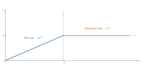
Figure 2: Exponent $p$ appearing in the rates of convergence $n^{-p}$ in Theorem 4 as a function of the smoothness $\alpha$.

5 Some extensions

A slightly less precise but more general result can be obtained for any bounded class whose entropy grows polynomially in $1/\varepsilon$; see also Rakhlin et al., (2017, Theorem 2), where this condition naturally arises. Such an extension can be stated as follows.

Theorem 5.

Let $\mathcal{X}\subset\mathbb{R}^{d}$ be a convex bounded set with non-empty interior. Let $\mathcal{H}$ be a bounded class of functions supported on the set $\mathcal{X}$. Assume that the entropy of the class grows polynomially, i.e., there exist positive real numbers $p$ and $A$ such that

$$\forall\varepsilon>0,\quad\log\mathcal{N}(\mathcal{H},\lVert\cdot\rVert_{\infty},\varepsilon)\leq A\varepsilon^{-p}.$$ (28)

Then, for any probability distribution $P$ supported on $\mathcal{X}$, denoting by $P_{n}$ the empirical measure associated to i.i.d. samples $X_{1},\dots,X_{n}\sim P$, we have,

$$\mathbb{E}\big{[}d_{\mathcal{H}}(P_{n},P)\big{]}=\mathbb{E}\bigg{[}\sup_{h\in\mathcal{H}}\big{\lvert}\mathbb{X}_{n}(h)\big{\rvert}\bigg{]}\leq c\begin{cases}n^{-\nicefrac{{1}}{{p}}}&\text{if $p>2$},\\ n^{-\nicefrac{{1}}{{2}}}\ln(n)&\text{if $p=2$},\\ n^{-\nicefrac{{1}}{{2}}}&\text{if $p<2$},\end{cases}$$ (29)

where $c$ is a constant.

The proof of the extension is exactly the same as the proof of Theorem 4 up to constants. In this note we have seen Hölder classes as examples of classes with polynomial growth of the entropy but there are many other such classes. To illustrate this we give the example of Sobolev classes which, in some cases, are more general than Hölder classes. For a positive integer $s$ and a real number $1\leq p\leq+\infty$, define the Sobolev space $\mathcal{W}_{p}^{s}(r)$ with radius $r>0$ as

$$\mathcal{W}^{s}_{p}(r)\coloneqq\left\{f\in C^{s}(\mathcal{X},\mathbb{R}):\sum_{\lvert k\rvert\leq s}\lVert D^{k}f\rVert_{p}\leq r\right\}.$$ (30)

Note that for any positive integer $s$ and for any positive radius $L$, there exist radii $r$ and $r^{\prime}$ such that

$$\mathcal{W}^{s}_{\infty}(r)\subset\mathcal{H}^{s}(L)\subset\mathcal{W}^{s-1}_{\infty}(r^{\prime}).$$ (31)

A consequence of (Nickl and Pötscher,, 2007, Corollary 1) is that for any positive integer $s>0$, and real number $p$ such that $d/s<p\leq+\infty$, the entropy of a Sobolev class grows polynomially as

$$\log\mathcal{N}(\mathcal{W}^{s}_{p}(L),\lVert\cdot\rVert_{\infty},\varepsilon)\leq A\varepsilon^{-d/s},$$ (32)

for some positive constant $A$. Thus Theorem 5 holds for this class. Finally we point out that such bounds on the entropy hold for more general spaces such as some Besov spaces. We refer the reader to Nickl and Pötscher, (2007) for more details.

6 Appendix: proofs

This section contains the proofs of the main results, Theorems 3 and 4, stated in the main body of the note.

6.1 Proof of Theorem 3

The proof of Theorem 3 can be found in Srebro and Sridharan, (2010). We add it here for completeness.

Let $\gamma_{0}=S_{n}(\mathcal{F})=\sup_{f\in\mathcal{F}}\lVert f\rVert_{L_{2}(P_{n})}$. Define $\gamma_{j}=2^{-j}\gamma_{0}$, for every integer $j\in\mathbb{N}$, and let $T_{j}$ be a minimal $\gamma_{j}$-cover of $\mathcal{F}$ with respect to $L_{2}(P_{n})$. For any function $f\in\mathcal{F}$, we denote by $\widehat{f}_{j}$ an element of $T_{j}$ which is an $\gamma_{j}$ approximation of $f$. For any positive integer $N$ we can decompose the function $f$ as

$$f=f-\widehat{f}_{N}+\sum_{j=1}^{N}(\widehat{f}_{j}-\widehat{f}_{j-1})$$ (33)

where $\widehat{f}_{0}=0\in\mathcal{F}$. Hence, for any positive integer $N$, we have

$$\widehat{R}_{n}(\mathcal{F}) =\frac{1}{n}\mathbb{E}_{\sigma}\left[\sup_{f\in\mathcal{F}}\sum_{i=1}^{n}\sigma_{i}\left(f(X_{i})-\widehat{f}_{N}(X_{i})+\sum_{j=1}^{N}(\widehat{f}_{j}(X_{i})-\widehat{f}_{j-1}(X_{i}))\right)\right]$$ (34)

$$\leq\frac{1}{n}\mathbb{E}_{\sigma}\left[\sup_{f\in\mathcal{F}}\sum_{i=1}^{n}\sigma_{i}(f(X_{i})-\widehat{f}_{N}(X_{i}))\right]+\sum_{j=1}^{N}\frac{1}{n}\mathbb{E}_{\sigma}\left[\sup_{f\in\mathcal{F}}\sum_{i=1}^{n}\sigma_{i}(\widehat{f}_{j}(X_{i})-\widehat{f}_{j-1}(X_{i}))\right]$$ (35)

$$\leq\frac{1}{n}\sup_{f\in\mathcal{F}}\sum_{i=1}^{n}|(f(X_{i})-\widehat{f}_{N}(X_{i}))|+\sum_{j=1}^{N}\frac{1}{n}\mathbb{E}_{\sigma}\left[\sup_{f\in\mathcal{F}}\sum_{i=1}^{n}\sigma_{i}(\widehat{f}_{j}(X_{i})-\widehat{f}_{j-1}(X_{i}))\right]$$ (36)

$$=\sup_{f\in\mathcal{F}}\lVert f-\widehat{f}_{N}\rVert_{L_{2}(P_{n})}+\sum_{j=1}^{N}\frac{1}{n}\mathbb{E}_{\sigma}\left[\sup_{f\in\mathcal{F}}\sum_{i=1}^{n}\sigma_{i}(\widehat{f}_{j}(X_{i})-\widehat{f}_{j-1}(X_{i}))\right]$$ (37)

$$\leq\gamma_{N}+\sum_{j=1}^{N}\frac{1}{n}\mathbb{E}_{\sigma}\left[\sup_{f\in\mathcal{F}}\sum_{i=1}^{n}\sigma_{i}(\widehat{f}_{j}(X_{i})-\widehat{f}_{j-1}(X_{i}))\right].$$ (38)

For any positive integer $j$, the triangle inequality gives

$$\lVert\widehat{f}_{j}-\widehat{f}_{j-1}\rVert_{L_{2}(P_{n})}\leq\lVert\widehat{f}_{j}-f\rVert_{L_{2}(P_{n})}+\lVert f-\widehat{f}_{j-1}\rVert_{L_{2}(P_{n})}\leq\gamma_{j}+\gamma_{j-1}=3\gamma_{j}.$$ (39)

We need the following classic lemma which controls the expectation of a Rademacher average over a finite set.

Lemma 3 (Massart’s finite class lemma).

Let $\mathcal{X}$ be a finite subset of $\mathbb{R}^{n}$ and let $\sigma_{1},\dots,\sigma_{n}$ be independent Rademacher random variables. Denote the radius of $\mathcal{X}$ by $R=\sup_{x\in\mathcal{X}}\lVert x\rVert$. Then, we have,

$$\mathbb{E}\left[\sup_{x\in\mathcal{X}}\frac{1}{n}\sum_{i=1}^{n}\sigma_{i}x_{i}\right]\leq R\frac{\sqrt{2\log\lvert\mathcal{X}\lvert}}{n}.$$ (40)

Applying this lemma to $\mathcal{X}_{j}=\left\{(\widehat{f}_{j}(X_{i})-\widehat{f}_{j-1}(X_{i}))_{i=1}^{n}\in\mathbb{R}^{n}:f\in\mathcal{F}\right\}$ for any $j=1,\dots,n$ and using (39), we get

$$\sum_{j=1}^{N}\frac{1}{n}\mathbb{E}_{\sigma}\left[\sup_{f\in\mathcal{F}}\sum_{i=1}^{n}\sigma_{i}(\widehat{f}_{j}(X_{i})-\widehat{f}_{j-1}(X_{i}))\right]\leq\sum_{j=1}^{N}3\gamma_{j}\frac{\sqrt{2\log(\lvert T_{j}\rvert\cdot\rvert T_{j-1}\lvert)}}{n}$$ (41)

Therefore we have

$$\widehat{R}_{n}(\mathcal{F}) \leq\gamma_{N}+\sum_{j=1}^{N}3\gamma_{j}\frac{\sqrt{2\log(\lvert T_{j}\rvert\cdot\rvert T_{j-1}\lvert)}}{n}$$ (42)

$$\leq\gamma_{N}+\frac{6}{n}\sum_{j=1}^{N}\gamma_{j}\sqrt{\log\lvert T_{j}\rvert}$$ (43)

$$=\gamma_{N}+\frac{12}{n}\sum_{j=1}^{N}(\gamma_{j}-\gamma_{j+1})\sqrt{\log\lvert T_{j}\rvert}$$ (44)

$$=\gamma_{N}+\frac{12}{n}\sum_{j=1}^{N}(\gamma_{j}-\gamma_{j+1})\sqrt{\log\mathcal{N}(\mathcal{F},L_{2}(P_{n}),\gamma_{j})}$$ (45)

$$\leq\gamma_{N}+\frac{12}{n}\int_{\gamma_{N+1}}^{\gamma_{0}}\sqrt{\log\mathcal{N}(\mathcal{F},L_{2}(P_{n}),\varepsilon)}d\varepsilon.$$ (46)

For any $\tau>0$, pick $N=\sup\{j:\gamma_{j}>2\tau\}$. Then $\gamma_{N}=2\gamma_{N+1}\leq 4\tau$ and $\gamma_{N+1}=\gamma_{N}/2\geq\tau$. Hence, we conclude that

$$\widehat{R}_{n}(\mathcal{F})\leq 4\tau+\frac{12}{\sqrt{n}}\int_{\tau}^{\gamma_{0}}\sqrt{\log\mathcal{N}(\mathcal{F},L_{2}(P_{n}),\varepsilon)}\,d\varepsilon.$$ (47)

Since $\tau$ can take any positive value we can take the infimum over all positive $\tau$ and this concludes the proof.

6.2 Proof of Theorem 4

Without loss of generality, we prove the theorem in the case $L=1$. The general case will follow by homogeneity. For simplicity we write $\mathcal{H}^{\alpha}=\mathcal{H}^{\alpha}(1)$, $Ph=\int_{\mathcal{X}}h\,dP$ and $P_{n}h=\int_{\mathcal{X}}h\,dP_{n}$. A symmetrization argument (1) gives

$$\mathbb{E}\bigg{[}\sup_{h\in\mathcal{H}^{\alpha}}\lvert Ph-P_{n}h\rvert\bigg{]}\leq 2\mathbb{E}\big{[}\widehat{R}_{n}(\mathcal{H}^{\alpha})\big{]},$$ (48)

where the empirical Rademacher process $\widehat{R}_{n}(\mathcal{H}^{\alpha})$ is given by

$$\widehat{R}_{n}(\mathcal{H}^{\alpha})=\frac{1}{n}\mathbb{E}\left[\sup_{h\in\mathcal{H}^{\alpha}}\sum_{i=1}^{n}\sigma_{i}h(X_{i})\bigg{|}X_{1},\ldots,X_{n}\right].$$ (49)

Noting that, for any $h\in\mathcal{H}^{\alpha}$,

$$P_{n}h^{2}\coloneqq\frac{1}{n}\sum_{i=1}^{n}h^{2}(X_{i})\leq\lVert h^{2}\rVert_{\infty}\leq 1,$$ (50)

the improved Dudley bound (Theorem 3) coupled with 2 yields,

$$\mathbb{E}\bigg{[}\sup_{h\in\mathcal{H}^{\alpha}}\lvert P_{n}h-Ph\rvert\bigg{]} \leq\inf_{\tau>0}\left(4\tau+\frac{12}{\sqrt{n}}\int_{\tau}^{1}\sqrt{\log\mathcal{N}(\mathcal{H}^{\alpha},\lVert\cdot\rVert_{\infty},\varepsilon)}d\varepsilon\right)$$ (51)

$$\leq\inf_{\tau>0}\left(4\tau+\frac{12\sqrt{K\lambda_{d}(\mathcal{X}^{1})}}{\sqrt{n}}\int_{\tau}^{1}\varepsilon^{-d/2\alpha}d\varepsilon\right)$$ (52)

Applying 4 with $\beta=\frac{d}{2\alpha}$ and $a=3\sqrt{\frac{K\lambda}{n}}$ where $K=K_{\alpha,d}$ is the constant depending only on $\alpha$ and $d$ borrowed from Theorem 1 and $\lambda\coloneqq\lambda_{d}(\mathcal{X}^{1})$, we get

$$\mathbb{E}\bigg{[}\sup_{h\in\mathcal{H}^{\alpha}}\lvert P_{n}h-Ph\rvert\bigg{]}\leq 12\begin{cases}\left(\frac{K\lambda}{n}\right)^{\nicefrac{{\alpha}}{{d}}}\left[\frac{d}{d-2\alpha}\wedge(1+0.5\log(\frac{n}{9K\lambda}))\right]&\text{if $\alpha<\nicefrac{{d}}{{2}}$},\\[10.0pt] \left(\frac{K\lambda}{n}\right)^{\nicefrac{{1}}{{2}}}\left[\frac{2\alpha}{2\alpha-d}\wedge(1+\frac{\alpha}{d}\log(\frac{n}{9K\lambda}))\right]&\text{if $\alpha\geq\nicefrac{{d}}{{2}}$}.\end{cases}$$ (54)

The proof is finished since the upper bound stated in Theorem 4 is a direct consequence of (54)

6.3 Additional lemma

The following lemma enables to obtain an upper bound on Dudley’s refined bound (Theorem 3) for any bounded class whose entropy grows polynomially in $1/\varepsilon$.

Lemma 4.

For any real positive numbers $a$ and $\beta$, it holds

$$\min_{0\leq\tau\leq 1}\left(\tau+a\int_{\tau}^{1}\varepsilon^{-\beta}d\varepsilon\right)\leq(a^{\nicefrac{{1}}{{\beta}}}\vee a)\left[\left(\frac{\beta\vee 1}{\lvert\beta-1\rvert}\right))\wedge\left(1+\frac{\log(\nicefrac{{1}}{{a}})}{\beta\vee 1}\right)\right].$$ (55)

Proof.

Let $a$ and $\beta$ be real positive numbers. Define the function

$$f\colon[0,1] \to\mathbb{R}$$ (56)

$$\tau \mapsto\tau+a\int_{\tau}^{1}\varepsilon^{-\beta}d\varepsilon.$$ (57)

One can easily check that

$$f^{*}\coloneqq\min_{0\leq\tau\leq 1}f(\tau)=\begin{cases}1&\text{if $a>1$},\\ a^{\nicefrac{{1}}{{\beta}}}+\frac{a}{1-\beta}(1-a^{\nicefrac{{1}}{{\beta}}-1})&\text{if $a<1$ }.\end{cases}$$ (58)

In the case $a<1$, using the fact that $1-x^{\alpha}\leq\log(x^{-\alpha})$ for any $\alpha>0$ and $x\in(0,1]$, we have

$$f^{*}\leq(a^{\nicefrac{{1}}{{\beta}}}\vee a)\left[\left(\frac{\beta\vee 1}{\lvert\beta-1\rvert}\right))\wedge\left(1+\frac{\log(\nicefrac{{1}}{{a}})}{\beta\vee 1}\right)\right].$$ (59)

Finally, since the RHS of (59) is greater than $1$ for any $a>1$, (59) holds for any positive real $a$ and this concludes the proof. ∎

References

- Arjovsky et al., (2017) Arjovsky, M., Chintala, S., and Bottou, L. (2017). Wasserstein generative adversarial networks. In Precup, D. and Teh, Y. W., editors, Proceedings of the 34th International Conference on Machine Learning, volume 70 of Proceedings of Machine Learning Research, pages 214–223, International Convention Centre, Sydney, Australia. PMLR.
- Bassetti et al., (2006) Bassetti, F., Bodini, A., and Regazzini, E. (2006). On minimum Kantorovich distance estimators. Statistics & probability letters, 76(12):1298–1302.
- Briol et al., (2019) Briol, F.-X., Barp, A., Duncan, A. B., and Girolami, M. (2019). Statistical inference for generative models with maximum mean discrepancy. arXiv preprint arXiv:1906.05944.
- Chen et al., (2020) Chen, M., Liao, W., Zha, H., and Zhao, T. (2020). Statistical guarantees of generative adversarial networks for distribution estimation. arXiv preprint arXiv:2002.03938.
- del Barrio et al., (2007) del Barrio, E., Deheuvels, P., and van de Geer, S. (2007). Lectures on empirical processes. EMS Series of Lectures in Mathematics. European Mathematical Society (EMS), Zürich. Theory and statistical applications, With a preface by Juan A. Cuesta Albertos and Carlos Matrán.
- Dudley, (1968) Dudley, R. M. (1968). The speed of mean Glivenko-Cantelli convergence. Ann. Math. Statist., 40:40–50.
- Giné and Nickl, (2016) Giné, E. and Nickl, R. (2016). Mathematical foundations of infinite-dimensional statistical models, volume 40. Cambridge University Press.
- Goodfellow et al., (2014) Goodfellow, I., Pouget-Abadie, J., Mirza, M., Xu, B., Warde-Farley, D., Ozair, S., Courville, A., and Bengio, Y. (2014). Generative adversarial nets. In Advances in neural information processing systems, pages 2672–2680.
- Koltchinskii, (2011) Koltchinskii, V. (2011). Oracle Inequalities in Empirical Risk Minimization and Sparse Recovery Problems: Ecole d’Eté de Probabilités de Saint-Flour XXXVIII-2008, volume 2033. Springer Science & Business Media.
- Liang, (2018) Liang, T. (2018). On how well generative adversarial networks learn densities: Nonparametric and parametric results. arXiv preprint arXiv:1811.03179.
- Nickl and Pötscher, (2007) Nickl, R. and Pötscher, B. M. (2007). Bracketing metric entropy rates and empirical central limit theorems for function classes of besov-and sobolev-type. Journal of Theoretical Probability, 20(2):177–199.
- Rakhlin et al., (2017) Rakhlin, A., Sridharan, K., and Tsybakov, A. B. (2017). Empirical entropy, minimax regret and minimax risk. Bernoulli, 23(2):789–824.
- Santambrogio, (2015) Santambrogio, F. (2015). Optimal transport for applied mathematicians. Birkäuser, NY, 55(58-63):94.
- Scetbon et al., (2020) Scetbon, M., Meunier, L., Atif, J., and Cuturi, M. (2020). Equitable and optimal transport with multiple agents. arXiv preprint arXiv:2006.07260.
- Shiryayev, (1993) Shiryayev, A. (1993). Selected Works of AN Kolmogorov: Volume III: Information Theory and the Theory of Algorithms, volume 27. Springer.
- Srebro and Sridharan, (2010) Srebro, N. and Sridharan, K. (2010). Note on refined Dudley integral covering number bound. Unpublished results. http://ttic. uchicago. edu/karthik/dudley. pdf.
- Srebro et al., (2010) Srebro, N., Sridharan, K., and Tewari, A. (2010). Smoothness, low noise and fast rates. In Advances in neural information processing systems, pages 2199–2207.
- Sriperumbudur et al., (2012) Sriperumbudur, B. K., Fukumizu, K., Gretton, A., Schölkopf, B., Lanckriet, G. R., et al. (2012). On the empirical estimation of integral probability metrics. Electronic Journal of Statistics, 6:1550–1599.
- Tsybakov, (2008) Tsybakov, A. B. (2008). Introduction to nonparametric estimation. Springer Science & Business Media.
- van der Vaart and Wellner, (1996) van der Vaart, A. W. and Wellner, J. A. (1996). Weak convergence and empirical processes. Springer Series in Statistics. Springer-Verlag, New York. With applications to statistics.
- Vershynin, (2018) Vershynin, R. (2018). High-dimensional probability: An introduction with applications in data science, volume 47. Cambridge university press.
- Weed et al., (2019) Weed, J., Bach, F., et al. (2019). Sharp asymptotic and finite-sample rates of convergence of empirical measures in wasserstein distance. Bernoulli, 25(4A):2620–2648.