Abstract

We propose a model for the universe based on Jordan algebras. The action consists of cubic terms with coefficients being the structure constants of a Jordan algebra. Coupling constants only enter the theory via symmetry breaking which also selects a physical vacuum. “Before” the symmetry breaking the universe is in a pre-geometric state where it makes no sense to talk about space or time, but time comes into existence with the symmetry breaking together with a Hamiltonian which can create space from “nothing” and in some cases can propagate the space to macroscopic size in a finite time. There exists symmetry breaking which results in macroscopic spacetime dimensions 3, 4, 6 and 10, based on the Jordan algebras of Hermitian 3x3 matrices with real, complex, quarternion and octonion entries, respectively.

PACS codes: 11.25.Pm, 11.25.Sq and 04.60.$-$m

Keywords: Quantum gravity

1 Introduction

Observations indicate that our present universe is expanding and that it at an earlier stage has been much smaller and hotter than today. A theory of our universe should preferable explain what happened before this early and hot time. One scenario which brings us further back in time is the concept of inflation. This scenario was invented to solve a number of issues related to a Big Bang theory which naively extrapolated the hot and small universe which once existed further backwards in time. However, the concept of inflation still leaves unanswered what happened before inflation: can one at all speak of space and time when the universe is of “Planck scale”, and if not, what kind of theory can one image leads to our present universe. The purpose of this article is to present a model with allows us to address such questions. Needless to say it will not answer the questions in a completely satisfactory way, but we nevertheless feel that it is important to address such questions if we believe that there is an underlying theory from which the behaviour of our universe can be derived in some way. One interesting aspect of the model is that it links properties of the universe at the shortest scales, namely the possibility of the universe to change topology by quantum fluctuations, to the acceleration of the universe observed today. Another interesting aspect of the model is that it presents a scenario where the “universe” is naturally in a pre-geometric, very symmetric state where it makes no sense to talk about time and spatial geometry. After symmetry breaking there is then the possibility of emergence of time and an associated Hamiltonian and after that of spatial geometry and thus the emergence of a “universe” which may resemble our universe. Different kinds of “universes” might emerge from different patterns of symmetry breaking, and one intriguing possibility is a universe with 9 extended and 16 small, compact spatial dimensions, a situation similar to what occurs for the heterotic string. It is also possible to obtain a universe with three extended spatial dimensions, while the rest are small and compact.

In the pre-geometric phase there is no concept of time and thus no concept of unitary evolution. This has the consequence that the symmetry breaking results in the emergence of time and an associated Hamiltonian which is not entirely Hermitian: it is possible to create spatial universes of infinitesimal extension. Such universes can grow with time and they can merge and split and eventually evolve to something resembling our universe. Under suitable assumptions one can then derive a modified Friedmann equation for such a universe, which, as already mentioned, links the future acceleration to the coupling constant responsible for splitting and merging of universes.

We were led to the present model by the study of causal dynamical triangulations (CDT). It is a non-perturbative lattice model of quantum gravity. In four dimensions the model can be studied by Monte Carlo simulations (see [1, 2] for reviews, [3] for orginal articles and [4] for recent results). However, in two dimensions (one space and one time dimension) the lattice model can be solved analytically and a continuum limit can be taken [5]. The continuum limit turns out to be a simple version [6] of Horava-Lifshitz gravity [7]. However, there is an generalisation of two-dimensional CDT which allows for topology change of space-time [8]. This generalisation can be formulated as a string field theory [9] which is quite similar to the standard non-critical string field theory [10, 11], just simpler since the kinetic term for string propagation is not singular in CDT string field theory, contrary to the situation for standard non-critical string field theory. Both CDT string field theory and non-critical string field theory describes how the string can split and joining, or in the context of two-dimensional quantum gravity how a spatial (one-dimensional) universe can split and join. However, these theories tell us surprisingly little about the creation of a universe from “nothing”, the confusing question we are confronted with in cosmology when we extrapolate backwards in time. It is well known that there is a $W_{3}$ symmetry underlying the standard non-critical string theory [12, 11]. In [13] we showed that one can also associate a $W_{3}$ symmetry with CDT string field theory, but the difference to non-critical string field theory was that insisting on a $W_{3}$ symmetric action from the beginning leads to a CDT string field theory which allows for the creation of spatial universes of infinitesimal size from the vacuum. In [14] this approach was generalized to include models with exended $W_{3}$ algebra symmetry, various space dimensions being assigned different “flavours”. In this way one can create higher dimensional space from “nothing”, and potentially created space-times which resemble our present universe. In our model the concept of inflation is somewhat different from the usual concept. Our model does not need an inflaton field, but is nevertheless able to solve the horizon problem, which is the most serious problem that the inflation models solve. It is also solves the flatness problem. It has nothing to say about the monopole problem, but there is of course only a monopole problem if there exists a suitable grand unified quantum field theory, which is maybe not so obvious any longer.

The purpose of this article is to provide some of the details of this model. Part of the present work has been published in short articles earlier [13, 14]. The rest of the article is organized as follows: In Sec. 2 we describe CDT string field theory, its relation to the $W^{(3)}$ algebra and how this gives rise to the emergence of time and space. In Sec. 3 we we describe Jordan algebras and their relation to extended $W^{(3)}$ algebras. In Sec. 4 we discuss some concrete models. Sec. 5 deals with the dynamics which can create higher dimensional universes from two-dimensional CDT universes with different “flavours”. Finally Sec. 6 contains a discussion of the results obtained so far.

2 Two-dimensional CDT gravity

2.1 Non-interacting CDT

The theory of causal dynamical triangulations in two dimensions was first formulated in [5] where the lattice theory was solved explicitly. The continuum limit of the lattice theory was found. It describes (in continuum notation) the amplitude for a spatial universe of size $L$ to propagate to a spatial universe of size $L^{\prime}$, the propagation taking a proper time $T$. This amplitude, or propagator, $G(L,L^{\prime},T)$ satisfies the follow differential equation

$$\frac{\partial}{\partial T}G(L,L^{\prime};T)=-H_{0}G(L,L^{\prime};T),\qquad H_{0}=L{\hskip 0.55603pt}\bigg{(}\!-\frac{\partial^{2}}{\partial L^{2}}+\mu\bigg{)}.$$ (2.1)

Figure 2.1: A typical configuration appearing in the path integral of the Green function. The arrow describes the direction of time $T$. The entrance loop has length $L$ and a marked point and the exit loop has length $L^{\prime}$ and no marked points.

In the path integral used for calculating the propagator $G(L,L^{\prime},T)$ one integrates over all two-dimensional geometries where the two space-like boundaries of lengths $L$ and $L^{\prime}$ are separated by proper time $T$ and where the topology of spacetime is that of a cylinder. Finally one assumes that the entrance loop with length $L$ has a marked point and the the initial condition when $T\to 0$ is

$$G(L,L^{\prime};0)\,=\,\delta(L-L^{\prime}).$$ (2.2)

A typical geometry associated with the propagator or Green function is illustrated in Fig. 2.1. The solution to this differential equation is

$$G(L,L^{\prime};T)\,=\,\frac{e^{-\sqrt{\mu}\,(L+L^{\prime})\coth(\sqrt{\mu}\,T)}}{\sinh(\sqrt{\mu}\,T)}\sqrt{\frac{\mu L}{L^{\prime}}}I_{1}\!\!\;\bigg{(}\frac{2\sqrt{\mu LL^{\prime}}}{\sinh(\sqrt{\mu}\,T)}\bigg{)}.$$ (2.3)

Using the Green function we can obtain various amplitudes of interest, which we will now discuss. The first is the so-called disk amplitude $F_{1}^{(0)}(L)$ obtained by contracting the exit loop to a point, i.e. taking $L^{\prime}\to 0$, and integrating over $T$

$$F_{1}^{(0)}(L)\,=\,\int\limits_{0}^{\infty}{\rm d}T\,G(L,0{\hskip 0.55603pt};T)\,=\,e^{-\sqrt{\mu}{\hskip 0.38922pt}L}\,.$$ (2.4)

(See Figure 2.2.)

Figure 2.2: A typical configuration of disk amplitude. The arrow describes the direction of time $T$. The entrance loop has length $L$ with a marked point.

Let us denote the size (the length) of the entrance loop $L_{0}$ and the size of the exit loop $L$. For $L_{0}\to 0$ one obtains the amplitude of the universe after what we denote “Big Bang”, i.e. the amplitude as a function of $T$ after the universe starts out with zero extension at $T=0$,

$$G_{\rm BB}(L;T)\! := \!\lim_{L_{0}\to 0}\frac{1}{L_{0}}\!\;G(L_{0},L;T)\,=\,\frac{\mu{\hskip 1.11206pt}e^{-\sqrt{\mu}\,L\coth(\sqrt{\mu}\,T)}}{\sinh^{2}(\sqrt{\mu}\,T)}.$$ (2.5)

The reason we divide by $L_{0}$ in the definition (2.5) is that a mark on the entrance boundary of length $L_{0}$ as shown in Fig. 2.1 has introduced such a factor in the first place and we have done that to be in accordance with the standard definition of the disk amplitude.

If we have a universe which at time $T=0$ has length $L_{0}$, we can calculate the expectation value of the length (i.e. the expectation value of the size of the universe) at $T$:

$$\langle L\rangle_{(L_{0},T)}\,:=\,\frac{\int_{0}^{\infty}dL{\hskip 1.11206pt}L{\hskip 0.55603pt}G(L_{0},L;T)}{\int_{0}^{\infty}dL{\hskip 1.11206pt}G(L_{0},L;T)}\,,$$ (2.6)

As shown in Appendix A we obtain

$$\langle L\rangle_{(L_{0},T)}\! = \!\frac{L_{0}}{\cosh^{2}(\sqrt{\mu}\,T)\big{(}1-e^{-2\sqrt{\mu}\,L_{0}/\sinh(2\sqrt{\mu}\,T)}\big{)}}\,,$$ (2.7)

and especially, for $L_{0}\!=\!0$, we have

$$\langle L\rangle_{(0,T)}\! = \!\frac{\tanh(\sqrt{\mu}\,T)}{\sqrt{\mu}}\,.$$ (2.8)

This gives the average size of space at time $T$ after the Big Bang. For short time $T$, (2.8) behaves as $\langle L\rangle_{(0,T)}=T+O(T^{3})$. This implies that the curvature at the birth of the universe is finite. It is seen that already when $T$ is of the order of $\frac{1}{\sqrt{\mu}}$ after the Big Bang, the size of space is close to its maximum value $L_{\rm cs}:=\frac{1}{\sqrt{\mu}}$. Finally we can ask for the amplitude that such a Big Bang universe vanishes at time $T$:

$$\lim_{L_{0}\to 0}\lim_{L\to 0}\frac{1}{L_{0}}{\hskip 1.11206pt}G(L_{0},L;T)\,=\,\frac{\mu}{\sinh^{2}(\sqrt{\mu}\,T)}\,.$$ (2.9)

Below we will also need the corresponding results when $\mu$ is negative. The details are provided in Appendix A. Here we just state the results:

$$G(L_{0},L;T)\,=\,\frac{e^{-\sqrt{-\mu}\,(L_{0}+L)\cot(\sqrt{-\mu}\,T)}}{\sin(\sqrt{-\mu}\,T)}\,\sqrt{\frac{-\mu L_{0}}{L}}\;I_{1}\!\!\;\bigg{(}\frac{2\sqrt{-\mu L_{0}L}}{\sin(\sqrt{-\mu}\,T)}\bigg{)}.$$ (2.10)

$$G_{\rm BB}(L;T)\! = \!\frac{-\mu{\hskip 1.11206pt}e^{-\sqrt{-\mu}\,L\cot(\sqrt{-\mu}\,T)}}{\sin^{2}(\sqrt{-\mu}\,T)}\,.$$ (2.11)

$$\langle L\rangle_{(0,T)}\! = \!\frac{\tan(\sqrt{-\mu}\,T)}{\sqrt{-\mu}}\,.$$ (2.12)

$$\lim_{L_{0}\to 0}\lim_{L\to 0}\frac{1}{L_{0}}{\hskip 1.11206pt}G(L_{0},L;T)\,=\,\frac{-\mu}{\sin^{2}(\sqrt{-\mu}\,T)}\,.$$ (2.13)

It is seen that a negative $\mu$ results in “inflation”: the universe is expanding as a function of $T$ and for $T=T_{\rm ps}:=\frac{\pi}{2\sqrt{-\mu}}$ it reaches infinite spatial size. We will later argue that in an interacting theory it does not imply that the theory breaks down for values of $T>T_{\rm ps}$, but rather that Coleman’s mechanism [15] forces the effective value of $\mu$ to be close to zero.

2.2 Second quantization

We can now introduce a “second quantized” notation and the corresponding Fock space, much like in many body theory. We let $H_{0}$ from (2.1) denote the “single (spatial) universe” Hamiltonian or single (closed) string Hamiltonian, in analogy with a single particle Hamiltonian in many body theory. Let $\Psi^{\dagger}(L)$ and $\Psi(L)$ be operators which create and annihilate one closed string with length $L$, respectively. More precisely $\Psi^{\dagger}(L)$ creates one closed string with a marked point, and $\Psi(L)$ annihilates one closed string with no marked points. The commutation relations of the string operators are

$$\big{[}\,\Psi(L)\,,\Psi^{\dagger}(L^{\prime})\,\big{]}\,=\,\delta(L-L^{\prime})\,,$$ (2.14)

$$\big{[}\,\Psi(L)\,,\Psi(L^{\prime})\,\big{]}\,=\,\big{[}\,\Psi^{\dagger}(L)\,,\Psi^{\dagger}(L^{\prime})\,\big{]}\,=\,0\,.$$ (2.15)

The vacuum states (no string states, in analogy with the no particle states in many body theory) $|{\rm vac}\rangle$ and $\langle{\rm vac}|$ are the Fock states defined by

$$\Psi(L)|{\rm vac}\rangle\,=\,\langle{\rm vac}|\Psi^{\dagger}(L)\,=\,0\,.$$ (2.16)

In this second quantized Hamiltonian formalism the Green function $G(L,L^{\prime};T)$ is obtained by

$$G(L,L^{\prime};T)\,=\,\langle{\rm vac}|\Psi(L^{\prime}){\hskip 1.11206pt}e^{-T{\cal H}_{\rm disk}}\Psi^{\dagger}(L)|{\rm vac}\rangle,\,.$$ (2.17)

where ${\cal H}_{\rm disk}$ consists of a tapole term and the kinetic term:

$${\cal H}_{\rm disk}\,=\,{\cal H}_{\rm tad}+{\cal H}_{0}$$ (2.18)

$${\cal H}_{\rm tad}=-\int\limits_{0}^{\infty}\!dL{\hskip 1.11206pt}\delta(L){\hskip 0.55603pt}\Psi(L),\qquad{\cal H}_{0}=\int\limits_{0}^{\infty}\!\frac{dL}{L}{\hskip 1.11206pt}\Psi^{\dagger}(L){\hskip 0.55603pt}H_{0}\,L\Psi(L)\,.$$ (2.19)

For the purpose of calculating $G(L,L^{\prime},T)$ one does not need the tadpole term in (2.18). However, if we want to reproduce the disk amplitude (2.4) directly in the second quantised formalism we need a closed string of length zero to have the possibility of disappearing into the vacuum. Including the tadpole term we can write

$$F_{1}^{(0)}(L)\,=\,\lim_{T\rightarrow\infty}\langle{\rm vac}|{\hskip 0.55603pt}e^{-T{\cal H}_{\rm disk}}\Psi^{\dagger}(L)|{\rm vac}\rangle\,.$$ (2.20)

Using that the right-hand side of eq. (2.20) converges to the left-hand side of eq. (2.20) which is independent of $T$, we have

$$\lim_{T\rightarrow\infty}\frac{\partial}{\partial T}\langle{\rm vac}|{\hskip 0.55603pt}e^{-T{\cal H}_{\rm disk}}\Psi^{\dagger}(L)|{\rm vac}\rangle\,=\,0\,.$$ (2.21)

This equation is equivalent to the so-called Schwinger-Dyson equation derived directly from CDT when one allows a spatial universe to split in two [8].

2.3 Interacting CDT: String Field Theory

One advantage of the second quantisation formalism in many body theory is that interaction between different particles is easily included in such a way that the statistics of many particles is automatically accounted for. The same is true when the particles are replaced by closed strings. If we assume that the interaction is that one string can split in two or two strings can merge into one, we can write the complete CDT string field Hamiltonian as

$${\cal H}\! = \!{\cal H}_{\rm disk}$$ (2.22)

$$\!-\;g\!\int\limits_{0}^{\infty}\!dL_{1}\!\int\limits_{0}^{\infty}\!dL_{2}{\hskip 1.11206pt}\Psi^{\dagger}(L_{1}){\hskip 0.55603pt}\Psi^{\dagger}(L_{2}){\hskip 0.55603pt}(L_{1}{}+{}L_{2})\Psi(L_{1}{}+{}L_{2})$$

$$\!-\;G{\hskip 0.55603pt}g\!\int\limits_{0}^{\infty}\!dL_{1}\!\int\limits_{0}^{\infty}\!dL_{2}{\hskip 1.11206pt}\Psi^{\dagger}(L_{1}{}+{}L_{2}){\hskip 0.55603pt}L_{1}\Psi(L_{1}){\hskip 0.55603pt}L_{2}\Psi(L_{2})\,.$$

The coupling constant $g$ counts the combined number of times strings will split or join while $G$ counts the handles (genus) of the spacetime created by the string. The Hamiltonian (2.22) can be derived from so-called generalized two-dimensional CDT [8]. The dynamics of spacetime created by the Hamiltonian (2.22) is illustrated in Fig. 2.3.

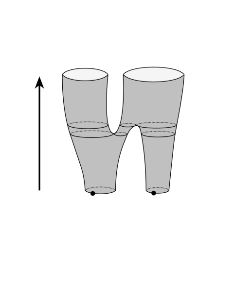
Figure 2.3: Dynamics of two spatial universes according to (2.22). At time $T=0$ we have two spatial universes. Both propagate according to the first term in (2.22). At a later time the left universe splits into two according to the second term in (2.22). Then one of these universes merges with the universe at the right of the picture, according to the third term in (2.22), and after that the universes propagate according to the first term in (2.22).

The Hamiltonian ${\cal H}$ is defined such that it satisfies

$${\cal H}{\hskip 0.55603pt}|{\rm vac}\rangle\,=\,0\,.$$ (2.23)

This condition expresses that the vacuum is stable under the time evolution generated by ${\cal H}$.

The model does not have time reversal symmetry. However, under the transformation

$$\Psi^{\dagger}(L)\,\leftrightarrow\,G\,L\Psi(L)$$ (2.24)

the only term in ${\cal H}$ not compatible with time reversal symmetry is the the tadpole term in (2.18).

As a generalisation of the disk amplitude (2.20) one can define the amplitude for merging many entrance loops, where the corresponding spacetime can have any topology by

$$\sum_{h=0}^{\infty}G^{{\hskip 0.38922pt}h+N-1}\,F_{N}^{(h)}(L_{1},\ldots,L_{N})\! = \!\lim_{T\rightarrow\infty}\langle{\rm vac}|{\hskip 0.55603pt}e^{-T{\cal H}}\Psi^{\dagger}(L_{1})\ldots\Psi^{\dagger}(L_{N})|{\rm vac}\rangle\,.$$

In eq. (2.3) $N$ denotes the number of entrance loops and $h$ the number of handles (i.e. the genus) of the spacetime. The generalisation of (2.21) is then

$$\lim_{T\rightarrow\infty}\frac{\partial}{\partial T}\langle{\rm vac}|{\hskip 0.55603pt}e^{-T{\cal H}}\Psi^{\dagger}(L_{1})\ldots\Psi^{\dagger}(L_{N})|{\rm vac}\rangle\,=\,0\,.$$ (2.26)

In the following it will be convenient to introduce the Laplace transformation of $\Psi^{\dagger}(L)$ and $\Psi(L)$ as

$$\tilde{\Psi}^{\dagger}(\xi)\,=\,\int\limits_{0}^{\infty}\!dL\,e^{-L\xi}{\hskip 0.55603pt}\Psi^{\dagger}(L)\,,\qquad\tilde{\Psi}(\eta)\,=\,\int\limits_{0}^{\infty}\!dL\,e^{-L\eta}{\hskip 0.55603pt}\Psi(L)\,.$$ (2.27)

Similarly, we also introduce the Laplace transformation for the other functions as

$$\tilde{G}(\xi,\eta;T)\,=\,\int\limits_{0}^{\infty}\!dL\!\int\limits_{0}^{\infty}\!dL^{\prime}\,e^{-L\xi-L^{\prime}\eta}{\hskip 0.55603pt}G(L,L^{\prime};T)\,,$$ (2.28)

$$\tilde{F}_{1}^{(0)}(\xi)\,=\,\int\limits_{0}^{\infty}\!dL\,e^{-L\xi}{\hskip 0.55603pt}F_{1}^{(0)}(L)\,,$$ (2.29)

and

$$\tilde{F}_{N}^{(h)}(\xi_{1},\ldots,\xi_{N})\,=\,\int\limits_{0}^{\infty}\!dL_{1}\ldots\!\int\limits_{0}^{\infty}\!dL_{N}\,e^{-L_{1}\xi_{1}-\ldots-L_{N}\xi_{N}}{\hskip 0.55603pt}F_{N}^{(h)}(L_{1},\ldots,L_{N})\,.$$ (2.30)

Then, the differential equation (2.1) and the initial condition (2.2) become

$$\frac{\partial}{\partial T}{\hskip 0.55603pt}\tilde{G}(\xi,\eta;T)\,=\,-(\xi^{2}-\mu)\frac{\partial}{\partial\xi}{\hskip 0.55603pt}\tilde{G}(\xi,\eta;T)\,,$$ (2.31)

and

$$\tilde{G}(\xi,\eta;0)\,=\,\frac{1}{\xi+\eta}\,.$$ (2.32)

The disk amplitude expressions (2.4) and (2.20) transform to

$$\tilde{F}_{1}^{(0)}(\xi)\,=\,\lim_{T\rightarrow\infty}\langle{\rm vac}|{\hskip 0.55603pt}e^{-T\tilde{{\cal H}}_{\rm disk}}\tilde{\Psi}^{\dagger}(\xi)|{\rm vac}\rangle\,=\,\frac{1}{\xi+\sqrt{\mu}}\,,$$ (2.33)

and the amplitudes with general topology (2.3) read

$$\sum_{h=0}^{\infty}G^{{\hskip 0.38922pt}h+N-1}\,\tilde{F}_{N}^{(h)}(\xi_{1},\ldots,\xi_{N})\! = \!\lim_{T\rightarrow\infty}\langle{\rm vac}|{\hskip 0.55603pt}e^{-T\tilde{{\cal H}}}\tilde{\Psi}^{\dagger}(\xi_{1})\ldots\tilde{\Psi}^{\dagger}(\xi_{N})|{\rm vac}\rangle\,,$$

where $\tilde{{\cal H}}_{\rm disk}=\tilde{{\cal H}}\big{|}_{g=0}$ and

$$\tilde{{\cal H}}\! = \!\!{\int\limits_{-i\infty}^{+i\infty}\frac{d\zeta}{2\pi i}}\,\Bigl{\{}-\,\tilde{\Psi}(-\zeta)\,-\,(\tilde{\Psi}^{\dagger}(\zeta))\big{(}\zeta^{2}-\mu\big{)}{\hskip 0.55603pt}\frac{\partial}{\partial\zeta}\tilde{\Psi}(-\zeta)$$ (2.35)

$$\!\!\phantom{{\int\limits_{-i\infty}^{+i\infty}\frac{d\zeta}{2\pi i}}\,\Bigl{\{}}\!\!{\hskip 1.11206pt}-\,g{\hskip 0.55603pt}(\tilde{\Psi}^{\dagger}(\zeta))^{2}\frac{\partial}{\partial\zeta}\tilde{\Psi}(-\zeta)\,-\,G{\hskip 0.55603pt}g{\hskip 0.55603pt}\tilde{\Psi}^{\dagger}(\zeta)\Bigl{(}\frac{\partial}{\partial\zeta}\tilde{\Psi}(-\zeta)\Bigr{)}^{2}\,\Bigr{\}}\,.\quad$$

This Hamiltonian can be obtained directly from (2.22).

If we introduce the generating function

$$Z_{F}[{\cal J}]\,\stackrel{{\scriptstyle\rm def}}{{\equiv}}\,\lim_{T\rightarrow\infty}\langle{\rm vac}|\,e^{-T\tilde{{\cal H}}}\exp\!\Big{\{}\int\!\frac{d\zeta}{2\pi i}\tilde{\Psi}^{\dagger}(\zeta){\cal J}(-\zeta)\Big{\}}|{\rm vac}\rangle\,,$$ (2.36)

the amplitudes with general topology (2.3) can be obtain in the standard way by functional differentiation after $\ln Z_{F}({\cal J})$:

$$\sum_{h=0}^{\infty}G^{{\hskip 0.38922pt}h+N-1}\tilde{F}_{N}^{(h)}(\xi_{1},\ldots,\xi_{N};\mu)\! = \!\frac{\delta^{N}}{\delta{\cal J}(\xi_{1})\,\cdots\,\delta{\cal J}(\xi_{N})}\ln Z_{F}[{\cal J}]\Bigg{|}_{{\cal J}=0}\,.\quad$$ (2.37)

Again, as in ordinary quantum field theory, the advantage of using the generating function $Z_{F}({\cal J})$ is that operators $A$ of $\Psi^{\dagger}$ and $\Psi$ acting $Z_{F}(J)$ can be expressed in terms of $\frac{\delta}{\delta{\cal J}}$ and ${\cal J}$. To be more explicit we associate with an operator $A$ of $\Psi^{\dagger}$ and $\Psi$ the operator $A^{\star}$ of $\frac{\delta}{\delta J}$ and $J$ defined by

$$A^{\star}Z_{F}[{\cal J}]\,=\,\lim_{T\rightarrow\infty}\langle{\rm vac}|\,e^{-T\tilde{{\cal H}}}A\exp\!\Big{\{}\int\!\frac{d\zeta}{2\pi i}\tilde{\Psi}^{\dagger}(\zeta){\cal J}(-\zeta)\Big{\}}|{\rm vac}\rangle\,.$$ (2.38)

For example,

$$\bigl{(}\tilde{\Psi}^{\dagger}(\xi)\bigr{)}^{\star}\,=\,\frac{\delta}{\delta{\cal J}(\xi)}\,,\qquad\bigl{(}\tilde{\Psi}(\eta)\bigr{)}^{\star}\,=\,{\cal J}(\eta)\,.$$ (2.39)

Under this so-called star operation, one finds the following property:

$$\bigl{(}A_{1}A_{2}\cdots A_{n}\bigr{)}^{\star}\,=\,A_{n}^{\star}\cdots A_{2}^{\star}{\hskip 0.55603pt}A_{1}^{\star}\,.$$ (2.40)

Using the star operation the Schwinger-Dyson equation (2.26) can be rewritten as

$$\tilde{{\cal H}}^{\star}Z_{F}[{\cal J}]\ =\ 0\,,$$ (2.41)

where

$$\tilde{{\cal H}}^{\star}\! = \!\!{\int\limits_{-i\infty}^{+i\infty}\frac{d\zeta}{2\pi i}}\Bigl{\{}\,-\,{\cal J}(-\zeta)\,-\,\Bigl{(}\frac{\partial}{\partial\zeta}{\cal J}(-\zeta)\Bigr{)}\big{(}\zeta^{2}-\mu\big{)}\Bigl{(}\frac{\delta}{\delta{\cal J}(\zeta)}\Bigr{)}$$

$$\!\!\phantom{{\int\limits_{-i\infty}^{+i\infty}\frac{d\zeta}{2\pi i}}\Bigl{\{}}\!\!{\hskip 1.11206pt}-\,g\Bigl{(}\frac{\partial}{\partial\zeta}{\cal J}(-\zeta)\Bigr{)}\Bigl{(}\frac{\delta}{\delta{\cal J}(\zeta)}\Bigr{)}^{2}\,-\,G{\hskip 0.55603pt}g\Bigl{(}\frac{\partial}{\partial\zeta}{\cal J}(-\zeta)\Bigr{)}^{2}\frac{\delta}{\delta{\cal J}(\zeta)}\,\Bigr{\}}\,.$$

2.4 The mode expansion of string field theory

We now introduce the so-called mode expansion. It is the mode expansion which allows us to relate CDT string field theory to $W$ symmetry in the most transparent way. For large $\xi$ the disk amplitude (2.33) has the expansion

$$\tilde{F}_{1}^{(0)}(\xi)\,=\,\xi^{-1}+\sum_{l=1}^{\infty}\xi^{-l-1}f_{1}^{(0)}(l)\,.$$ (2.43)

Similarly, the amplitudes with general topology have for large $\xi_{i}$ the expansion

$$\tilde{F}_{N}^{(h)}(\xi_{1},\ldots,\xi_{N})\,=\,\xi_{1}^{-1}\delta_{N,1}\delta_{h,0}\,+\sum_{l_{1},\ldots,l_{N}=1}^{\infty}\xi_{1}^{-l_{1}-1}\ldots\xi_{N}^{-l_{N}-1}f_{N}^{(h)}(l_{1},\ldots,l_{N})\,.$$ (2.44)

Note that the first term, $\xi^{-1}$, on the right-hand side of the last two equations does not contribute to the finite spacetime volume since it does not contain any reference to $\mu$. It can thus be considered as kind of non-universal term which we are free to choose in the mode expansion of the string fields. With this remark in mind we assume that the string fields have the following mode expansion

$$\tilde{\Psi}^{\dagger}(\xi)\,=\,\xi^{-1}+\sum_{l=1}^{\infty}\xi^{-l-1}\phi^{\dagger}_{l}\,,\qquad\tilde{\Psi}(\eta)=\sum_{l=1}^{\infty}(-\eta)^{l}\phi_{l}\,.$$ (2.45)

Using this mode expansion the commutation relations of string fields (2.14) and (2.15) become

$$\big{[}\,\phi_{l}\,,\phi^{\dagger}_{l^{\prime}}\,\big{]}\ =\ \delta_{l,l^{\prime}}\,,\qquad\big{[}\,\phi^{\dagger}_{l}\,,\phi^{\dagger}_{l^{\prime}}\,\big{]}\ =\ \big{[}\,\phi_{l}\,,\phi_{l^{\prime}}\,\big{]}\ =\ 0\,.$$ (2.46)

Substituting the string mode expansion (2.45) into the Hamiltonian (2.22) we obtain

$${\cal H}\! = \!\mu{\hskip 0.27802pt}\phi_{1}-\,2g{\hskip 0.27802pt}\phi_{2}\,-\,G{\hskip 0.55603pt}g{\hskip 0.27802pt}\phi_{1}\phi_{1}$$ (2.47)

$$\!-\>\sum_{l=1}^{\infty}\phi_{l+1}^{\dagger}l\phi_{l}\,+\,\mu\sum_{l=2}^{\infty}\phi_{l-1}^{\dagger}l\phi_{l}\,-\,2g\sum_{l=3}^{\infty}\phi_{l-2}^{\dagger}l\phi_{l}$$

$$\!-\>g\sum_{l=4}^{\infty}\sum_{n=1}^{l-3}\phi_{n}^{\dagger}\phi_{l-n-2}^{\dagger}l\phi_{l}$$

$$\!-\>G{\hskip 0.55603pt}g\sum_{l=1}^{\infty}\sum_{n=\max(3-l,1)}^{\infty}\phi_{n+l-2}^{\dagger}n\phi_{n}l\phi_{l}\,.$$

Note here that the term $2g\sum_{l=3}^{\infty}\phi_{l-2}^{\dagger}l\phi_{l}$ originates from the production of baby universes.

In particular we have for the non-interacting part of ${\cal H}$

$${\cal H}_{0}=\int\limits_{0}^{\infty}\!\frac{dL}{L}{\hskip 1.11206pt}\Psi^{\dagger}(L){\hskip 0.55603pt}H_{0}\,L\Psi(L)=-\sum_{l=1}^{\infty}\phi_{l+1}^{\dagger}l\phi_{l}+\mu\sum_{l=2}^{\infty}\phi_{l-1}^{\dagger}l\phi_{l}.$$ (2.48)

We have already seen that this part of the Hamiltonian is the one which determines the amplitude $G(L,L^{\prime},T)$ for a spatial universe of length $L$ to evolve into a spatial a universe of length $L^{\prime}$ in time $T$ without the spatial universe splitting in two or being joined by another spatial universe. From the explicit expression for $G(L,L^{\prime},T)$ it is seen that there is a non-zero amplitude for even a spatial universe of infinitesimal length space to expand to macroscopic size $L^{\prime}$ in a finite time $T$. Let us now consider a spatial universe in the quantum state $\phi^{\dagger}_{l}|{\rm vac}\rangle$. This is not a state where space has a specific length $L$. However, the distribution of lengths can be expressed in terms of $\delta(L)$ and derivatives of $\delta(L)$, i.e. $\phi^{\dagger}_{l}|{\rm vac}\rangle$ has to be assigned an infinitesimal length (distribution) for any finite mode number $l$. This is seen by working out the relation between the operators $\phi_{l},~{}\phi^{\dagger}_{l}$ and the operators $\Psi(L),~{}\Psi^{\dagger}(L)$ which annihilate and create spatial universes of macroscopic length $L$. We have

$$\Psi^{\dagger}(L)=\sum_{l=0}\frac{L^{l}}{l!}\;\phi^{\dagger}_{l},\qquad\phi^{\dagger}_{l}=\frac{d^{\,l}}{dL^{l}}\Psi^{\dagger}(L)\Big{|}_{L=0}.$$ (2.49)

The message to take along for the future discussion is that the kinetic term ${\cal H}_{0}$, given by the right hand side of eq. (2.48), is able to propagate a state of infinitesimal length like $|l\rangle=\phi^{\dagger}_{l}|{\rm vac}\rangle$ to a state of finite length $L^{\prime}$ within finite time $T$.

Introducing the mode expansion for the source term ${\cal J}(\eta)$, in analogy with the mode expansion (2.45) for $\Psi(\eta)$, i.e. ${\cal J}(\eta)=\sum_{l=1}^{\infty}(-\eta)^{l}j_{l}$, the generating function $Z_{F}[{\cal J}]$ (2.36) can be written as

$$Z_{f}[j]\,\stackrel{{\scriptstyle\rm def}}{{\equiv}}\,\lim_{T\rightarrow\infty}\langle{\rm vac}|\,e^{-T{\cal H}}\exp\!\Big{\{}\sum_{l=1}^{\infty}\phi^{\dagger}_{l}j_{l}\Big{\}}|{\rm vac}\rangle\,.$$ (2.50)

Then, the amplitudes $f_{N}^{(h)}$ defined in (2.44) can be obtain by differentiation after $\ln Z_{f}[j]$:

$$\sum_{h=0}^{\infty}G^{{\hskip 0.38922pt}h+N-1}f_{N}^{(h)}(l_{1},\ldots,l_{N})\! = \!\frac{\partial^{N}}{\partial j_{l_{1}}\,\cdots\,\partial j_{l_{N}}}\ln Z_{f}[j]\Bigg{|}_{j=0}\,.\quad$$ (2.51)

We can now apply the star operation (2.38) to the string modes. Using the mode decomposition, equation (2.38) now reads

$$A^{\star}Z_{f}[j]\,=\,\lim_{T\rightarrow\infty}\langle{\rm vac}|\,e^{-T{\cal H}}A\exp\!\Big{\{}\sum_{l=1}^{\infty}\phi^{\dagger}_{l}j_{l}\Big{\}}|{\rm vac}\rangle\,,$$ (2.52)

from which we obtain the analogy of (2.39)

$$\bigl{(}\phi^{\dagger}_{l}\bigr{)}^{\star}\ =\ \frac{\partial}{\partial j_{l}}\,,\qquad\bigl{(}\phi_{l}\bigr{)}^{\star}\ =\ j_{l}\,.$$ (2.53)

Thus the star operation applied to the Hamiltonian (2.47) leads to the following expression, which is the analogy of (2.3),

$${{\cal H}^{\star}}\! = \!\mu{\hskip 0.27802pt}j_{1}-\,2{\hskip 0.27802pt}gj_{2}\,-\,G{\hskip 0.55603pt}gj_{1}j_{1}$$ (2.54)

$$\!-\,\sum_{l=1}^{\infty}lj_{l}{\hskip 1.11206pt}\frac{\partial}{\partial j_{l+1}}\,+\,\mu\sum_{l=2}^{\infty}lj_{l}{\hskip 1.11206pt}\frac{\partial}{\partial j_{l-1}}\,-\,2g\sum_{l=3}^{\infty}lj_{l}{\hskip 1.11206pt}\frac{\partial}{\partial j_{l-2}}$$

$$\!-\>g\sum_{l=4}^{\infty}\sum_{n=1}^{l-3}lj_{l}{\hskip 1.11206pt}\frac{\partial}{\partial j_{n}}{\hskip 1.11206pt}\frac{\partial}{\partial j_{l-n-2}}$$

$$\!-\>G{\hskip 0.55603pt}g\sum_{l=1}^{\infty}\sum_{n=\max(3-l,1)}^{\infty}nj_{n}{\hskip 0.55603pt}lj_{l}{\hskip 1.11206pt}\frac{\partial}{\partial j_{n+l-2}}\,,$$

Corresponding to (2.41) we have

$${{\cal H}^{\star}}\;Z_{f}[j]=0.$$ (2.55)

It should be noted that three parameters $g$, $G$ and $\mu$ appear in CDT string field theory, while only $G$ and $\mu$ appear in conventional, $c=0$ non-critical string theory. The reason is that in $c=0$ non-critical string theory one can remove $g$ by a rescaling $T\to T/\sqrt{g}$, $\Psi^{\dagger}\to\Psi^{\dagger}/\sqrt{g}$, $\Psi\to\sqrt{g}\,\Psi$ and $G\to G/\sqrt{g}$ because $H_{0}=0$. This is impossible in CDT string field theory because $H_{0}\neq 0$.

2.5 The appearance of the W-algebra

The role of the $W$-algebra in non-critical string theory is well known [12, 11]. For a description which is closest to the one we will use here, we refer to [11]. For completeness let us define the $W^{(3)}$ algebra. Given a Fock space and operators $\alpha_{n}$ satisfying

$$[\alpha_{m},\alpha_{n}]=m\;\delta_{0,n+m},$$ (2.56)

we define

$$J(z)=\sum_{n\in Z}\frac{\alpha_{n}}{z^{n+1}},~{}~{}~{}~{}W^{(3)}(z)=\;\frac{1}{3}:J(z)^{3}:\;=\sum_{n\in Z}\frac{W^{(3)}_{n}}{z^{n+3}}.$$ (2.57)

The normal ordering $:\!(\cdot)\!:$ refers to the $\alpha_{n}$ operators ($\alpha_{n}$ to the left of $\alpha_{m}$ for $n<m$). We then have

$$W^{(3)}_{n}=\frac{1}{3}\sum_{a+b+c=n}:\alpha_{a}\alpha_{b}\alpha_{c}:.$$ (2.58)

In standard non-critical string theory for central charge $c=0$, i.e. the case of pure Euclidean two-dimensional quantum gravity, the Hamiltonian corresponding to our ${{\cal H}^{\star}}$ can be written as

$${{\cal H}^{\star}}\propto-\bar{W}^{(3)}_{-2}+Y,$$ (2.59)

where the $\alpha_{n}$ operators can be expressed in terms of $j_{n}$ and $\frac{\partial}{\partial j_{n}}$ and the operator $Y$ contains a few $\alpha_{n}$ needed to ensure the equivalent of (2.41) in the case of $c=0$ non-critical string theory. The bar over the $W$ in (2.59) refers to the fact that $W$-algebra which appears in standard non-critical string theory is a so-called 2-reduced $W$ algebra, which (loosely speaking) only involve the summation over even $n$ in formulas (2.57) and (2.58) (see [11] for precise definitions). The reason we recall these results from standard non-critical string theory is that we expect similar results for CDT string field theory, since the structure of this theory is quite similar to that of standard non-critical string theory (and, as already mentioned, in some sense simpler). Indeed, after a short calculation one finds that (2.54) can be expressed as

$${{\cal H}^{\star}}\! = \!-\,g\sqrt{G}\,W^{(3)}_{-2}\,+\,\frac{1}{G}\bigg{(}\frac{\mu^{2}}{4g}+\frac{1}{4g}\frac{\partial}{\partial j_{4}}-\frac{\mu}{2g}\frac{\partial}{\partial j_{2}}+\frac{\partial}{\partial j_{1}}\!\;\bigg{)}\,,$$ (2.60)

where, according to (2.58),

$$W^{(3)}_{-2}\ =\ \frac{1}{3}\sum_{k,l,m}\!:\!\alpha_{k}\alpha_{l}\alpha_{m}\!:\delta_{k+l+m,-2}=\mbox{res}_{z=0}\;W^{(3)}(z)\,,$$ (2.61)

and

$$\alpha_{n}:=\left\{\begin{array}[]{cl}\displaystyle\frac{1}{\sqrt{G}}{\hskip 1.11206pt}\frac{\partial}{\partial j_{n}}&\hbox{[\,$n\!>\!0$\,]}\rule[-12.0pt]{0.0pt}{30.0pt}\\ \displaystyle\nu&\hbox{[\,$n\!=\!0$\,]}\rule[-12.0pt]{0.0pt}{30.0pt}\\ \displaystyle-n(\lambda_{-n}+\sqrt{G}{\hskip 1.11206pt}j_{-n})&\hbox{[\,$n\!<\!0$\,]}\end{array}\right.$$ (2.65)

and

$$\nu=\frac{1}{\sqrt{G}}\,,\quad\lambda_{1}=-\,\frac{\mu}{2g{\sqrt{G}}}\,,\quad\lambda_{3}=\frac{1}{6g{\sqrt{G}}}\,,\quad\lambda_{n}=0,~{}~{}n\neq 1,3\,.$$ (2.66)

The Fock space where the $\alpha_{n}$ operators act is formed by suitable functions of the sequence $j_{n}$ by a standard construction.

Let us now use the (inverse) star operation to return from ${{\cal H}^{\star}}$ to ${\cal H}$ which is expressed in terms of string modes. First we apply the (inverse) star operation to $\alpha_{n}$:

$$\alpha_{n}=\left\{\begin{array}[]{cl}\displaystyle(a_{n}^{\dagger})^{\star}&\hbox{[\,$n\!>\!0$\,]}\rule[-12.0pt]{0.0pt}{30.0pt}\\ \displaystyle(p)^{\star}&\hbox{[\,$n\!=\!0$\,]}\rule[-12.0pt]{0.0pt}{30.0pt}\\ \displaystyle-n(a_{-n})^{\star}&\hbox{[\,$n\!<\!0$\,]}\end{array}\right.$$ (2.70)

The $a_{n}$ and $a^{\dagger}_{n}$ operators are related to our string modes $\phi_{n}$ and $\phi_{n}^{\dagger}$ by

$$a_{n}^{\dagger}\,=\,\frac{1}{\sqrt{G}}{\hskip 1.11206pt}\phi^{\dagger}_{n}\,,\qquad a_{n}\,=\,\lambda_{n}+\sqrt{G}{\hskip 1.11206pt}\phi_{n},$$ (2.71)

and with this notation the Hamiltonian (2.47) can be written as

$${\cal H}\! = \!g\sqrt{G}\,{\cal H}_{\rm W}\,+\,\frac{1}{G}\bigg{(}\frac{\mu^{2}}{4g}+\frac{1}{4g}\phi_{4}^{\dagger}-\frac{\mu}{2g}\phi_{2}^{\dagger}+\phi_{1}^{\dagger}\!\;\bigg{)}\,,$$ (2.72)

where ${\cal H}_{\rm W}$ is related to the $W^{(3)}_{-2}$-operator by an (inverse) star operation:

$${\cal H}_{\rm W}^{\star}\,=\,-W^{(3)}_{-2}=-\mbox{res}_{z=0}W^{(3)}(z)\,,$$ (2.73)

and explicitly one has

$${\cal H}_{\rm W}=-\!\!\!\!\!\!\sum_{\stackrel{{\scriptstyle\scriptstyle l,\,m,\,n}}{{[n+m+2=l\,]}}}\!\!\!\!a_{n}^{\dagger}a_{m}^{\dagger}la_{l}\;-\!\!\!\!\!\!\sum_{\stackrel{{\scriptstyle\scriptstyle n,\,m,\,l}}{{[n+2=m+l\,]}}}\!\!\!\!a_{n}^{\dagger}ma_{m}la_{l}-2\!\!\!\sum_{\stackrel{{\scriptstyle\scriptstyle n,\,l}}{{[n+2=l\,]}}}\!\!p\!\>a_{n}^{\dagger}la_{l}-p\!\>a_{1}a_{1}-2p^{2}a_{2}\,,$$ (2.74)

where the commutation relations are

$$\big{[}\,a_{m}\,,\,a_{n}^{\dagger}\,\big{]}=\delta_{m,n}\,,\qquad\quad\big{[}\,q\,,\,p\,\big{]}=i\,,$$ (2.75)

$$\big{[}\,p\,,\,a_{n}^{\dagger}\,\big{]}=\big{[}\,p\,,\,a_{n}\,\big{]}=\big{[}\,q\,,\,a_{n}^{\dagger}\,\big{]}=\big{[}\,q\,,\,a_{n}\,\big{]}=0\,,$$ (2.76)

and where we have introduced an operator $q$ which commutes with all $\alpha_{n}$ except $\alpha_{0}$. The pair $\alpha_{n},\alpha_{-n}$ is related to the creation and annihilation operator $a^{\dagger}_{n},a_{n}$ for $n>0$, while $\alpha_{0}=p$ is an Hermitian operator. Introducing $q$ allow us to talk about annihilation and creation operators also for the mode corresponding to $n=0$, precisely as for the ordinary harmonic oscillator if we define

$$a_{0}\,=\,\frac{1}{\sqrt{2}}(q+ip)\,,\qquad\quad a_{0}^{\dagger}\,=\,\frac{1}{\sqrt{2}}(q-ip)\,.$$ (2.77)

For furture reference we note that the eigenstates of $a_{0}$, i.e. states which satisfy $a_{0}|\lambda_{0}\rangle=\lambda_{0}|\lambda_{0}\rangle$, are related to the eigenstates of $p$, i.e. the states which satisfy $p|\nu\rangle=\nu|\nu\rangle$ by a standard formula from the theory of coherent states:

$$\langle\nu|\lambda_{0}\rangle=\exp\Big{(}-\frac{1}{2}(\sqrt{2}\lambda_{0}^{(i)}-\nu)^{2}+i(\sqrt{2}\lambda_{0}^{(i)}-\nu)\sqrt{2}\lambda_{0}^{(r)}\Big{)},$$ (2.78)

where $\lambda_{0}=\lambda_{0}^{(r)}+i\lambda_{0}^{(i)}$ and $\nu$ is real.

Note that ${\cal H}_{\rm W}$ does not contain any coupling constants when expressed in terms of the operators $p$, $a_{n}$ and $a_{n}^{\dagger}$ . Even the time $T$ placed in front of the Hamiltonian ${\cal H}_{\rm W}$ can be absorbed by the rescaling $\alpha_{n}\to T^{n/2}\alpha_{n}$.

2.6 Coherent states and the emergence of time and space

When two-dimensional CDT was formulated as a theory of quantum gravity the assumption was that there existed a stable vacuum state, $|{\rm vac}\rangle$, such that ${\cal H}|{\rm vac}\rangle=0$ (eq. (2.23)). However, if we assume that the relevant Hamiltonian is proportional to ${\cal H}_{\rm W}$, another state is the natural vacuum state, and we denote it the absolute vacuum $|0\rangle$. It satisfies

$$a_{n}|0\rangle=p|0\rangle=0\,,\qquad\quad\hbox{[\,$n\!=\!1$, $2$, \ldots\,]}\,,$$ (2.79)

and we have

$${\cal H}_{\rm W}|0\rangle=0.$$ (2.80)

The states in the Fock space ${\cal F}$ associated with ${\cal H}_{\rm W}$ are obtained by acting repeatedly on the absolute vacuum $|0\rangle$ with the operators $a_{n}^{\dagger}$ and $q$. If our stating point is just the algebraic structure dictated by the $\alpha_{n}$’s, we have no geometric interpretation of these states, and we denote them as “pre-geometric”. However, the vacuum state for ${\cal H}$ is a coherent state obtained from the absolute vacuum $|0\rangle$ in the following way

$$|\nu\rangle\,=\,{\rm e}^{i\nu q}|0\rangle\,,\qquad|{\rm vac}\rangle\,=\,V(\lambda_{1},\lambda_{3})|\nu\rangle\,,$$ (2.81)

$$V(\lambda_{1},\lambda_{3}):=\,\exp\!\bigg{(}\!-\frac{|\lambda_{1}|^{2}}{2}-\frac{|\lambda_{3}|^{2}}{2}+\lambda_{1}a_{1}^{\dagger}+\lambda_{3}a_{3}^{\dagger}\bigg{)}\,,$$ (2.82)

where $\lambda_{1}$ and $\lambda_{3}$ are given by (2.66), and where we have

$$a_{1}|{\rm vac}\rangle=\lambda_{1}|{\rm vac}\rangle\,,\qquad a_{3}|{\rm vac}\rangle=\lambda_{3}|{\rm vac}\rangle\,,\qquad p|{\rm vac}\rangle=\nu|{\rm vac}\rangle\,.$$ (2.83)

If we now assume that our system prefers $|{\rm vac}\rangle$ as the physical vacuum, we can put a geometrical interpretation into the various terms appearing in ${\cal H}_{W}$ via ${\cal H}$. ${\cal H}$ is an ordinary Hamiltonian, and we have seen that the states in the Hilbert space associated with ${\cal H}$ via its string field representation has a clear geometric interpretation. In addition we have a time evolution of these geometric states, governed by ${\cal H}$. The fact that $a_{1}$ and $a_{3}$ has an expectation value in the state $|{\rm vac}\rangle$, i.e. that $|{\rm vac}\rangle$ represents a condensate of $\phi_{1}$ and $\phi_{3}$ modes, implies that a quadratic term, namely the term ${\cal H}_{0}$ defined in (2.48), is created among the otherwise cubic interaction terms in ${\cal H}_{W}$. We know already the ${\cal H}_{0}$ can be associated with the propagation of states in ${\cal F}$ if we view $T$ as a time. The emergence of time is thus associated with the choice of a suitable coherent state in ${\cal F}$ which we denote the physical vacuum. The important difference between ${\cal H}$ and ${\cal H}_{\rm W}$ in this context is that ${\cal H}_{\rm W}|{\rm vac}\rangle\neq 0$: the last terms in the rhs of eq. (2.72) create universes of infinitesimal length, but the lengths of these universes will grow to macroscopic size because of the presence of ${\cal H}_{0}$. Thus we have the picture that a choice of $|{\rm vac}\rangle$ will first lead to the emergence of time, and successively to the emergence of space.

2.7 The interaction of two-dimensional W-universes

Once coupling constants associated with a universe are assigned in the manner described above, we are confronted with the situation that two universes with different coupling constants can merge into a third universe. This is a kind of generalised string field theory. Can we imagine some kind of interaction between states of different universes which governs such a merging? In order to suggest a suitable “vertex” for such an interaction we first establish a suitable notation for coherent states.

In ${\cal F}$ we can choose an (overcomplete) basis of coherent states as follows. Let us generalise the vertex operator (2.82) and introduce the corresponding coherent states

$$V[\lambda]:=V(\lambda_{0},\lambda_{1},\lambda_{2},\ldots)\,=\,\exp\!\bigg{(}\sum_{n=0}^{\infty}\lambda_{n}a_{n}^{\dagger}-\frac{1}{2}\sum_{n=0}^{\infty}\lambda_{n}^{2}\bigg{)}$$ (2.84)

and

$$|\lambda\rangle\!\rangle=V[\lambda]\;|0\rangle\!\rangle\,,$$ (2.85)

where the state $|0\rangle\!\rangle$ is defined by

$$a_{n}|0\rangle\!\rangle=0\quad{\rm for}\quad n=0,1,2,\ldots.$$ (2.86)

From (5.1) and the completeness relation for coherent states we have the following expression of the absolut vacuum $|0\rangle$ in terms of the coherent states $|\lambda\rangle\!\rangle$:

$$|0\rangle=\int\frac{d^{2}\lambda_{0}}{2\pi}|\lambda_{0},\lambda_{1}=0,\lambda_{2}=0,\ldots\rangle\!\rangle\;{\rm e}^{-\big{(}\big{(}\lambda_{0}^{(i)}\big{)}^{2}+\,i\lambda_{0}^{(i)}\lambda_{0}^{(r)}\big{)}}.$$ (2.87)

By declaring ${\cal H}_{W}$ the central object of our model, the absolut vacuum $|0\rangle$ as well as $|0\rangle\!\rangle$ become natural selected states in ${\cal F}$. From the properties of coherent states the overlap between states $|\lambda\rangle\!\rangle$ and $|\lambda^{\prime}\rangle\!\rangle$ will in general be non-zero and inspired by string field theory where two strings with different quantum numbers can join and form a string with new quantum numbers, or a string can split into two, also with different quantum numbers, we can imagine something similar here, the splitting and joining mediated by interactions

$$V_{-\langle} = \int\!\frac{{\rm d}^{2}\lambda}{\pi}\!\>\frac{{\rm d}^{2}\lambda^{\prime}}{\pi}\!\>\bigg{\{}e^{(\lambda+\lambda^{\prime})a^{\dagger}}|0\rangle\!\rangle\,\langle\!\langle 0|e^{\lambda^{\ast}a}\otimes\langle\!\langle 0|e^{\lambda^{\prime\ast}a}\bigg{\}}{\hskip 0.83405pt}e^{-|\lambda|^{2}-|\lambda^{\prime}|^{2}}\,,$$ (2.88)

$$V_{{\hskip 0.77844pt}\rangle-} = \int\!\frac{{\rm d}^{2}\lambda}{\pi}\!\>\frac{{\rm d}^{2}\lambda^{\prime}}{\pi}\!\>\bigg{\{}e^{(\lambda-\lambda^{\prime})a^{\dagger}}|0\rangle\!\rangle{}\otimes e^{\lambda^{\prime\ast}a^{\dagger}}|0\rangle\!\rangle\,\langle\!\langle 0|e^{\lambda^{{}\ast}a}\bigg{\}}{\hskip 0.83405pt}e^{-|\lambda|^{2}-|\lambda^{\prime}|^{2}}\,.$$ (2.89)

In these equations we have used the following notation

$$\frac{{\rm d}^{2}\lambda}{\pi}\,=\,\prod_{n=0}^{\infty}\frac{{\rm d}^{2}\lambda_{n}}{\pi}\,,\qquad\qquad e^{-|\lambda|^{2}}\,=\,\exp\!\bigg{(}\!\!-\!\sum_{n=0}^{\infty}|\lambda_{n}|^{2}\bigg{)}\,,$$ (2.90)

$$e^{\lambda a^{\dagger}}\,=\,\exp\!\bigg{(}\sum_{n=0}^{\infty}\lambda_{n}a_{n}^{\dagger}\bigg{)}\,,\qquad\quad e^{\lambda^{{}\ast}a}\,=\,\exp\!\bigg{(}\sum_{n=0}^{\infty}\lambda_{n}^{*}a_{n}\bigg{)}\,.$$ (2.91)

In these interaction vertices the total value of $\lambda$ (i.e. the sum of all $\lambda$’s) is preserved:

$$V_{-\langle}\,\big{(}{\hskip 1.11206pt}|\lambda_{0},\lambda_{1},\lambda_{2},\ldots\rangle\!\rangle\otimes|\lambda_{0}^{\prime},\lambda_{1}^{\prime},\lambda_{2}^{\prime},\ldots\rangle\!\rangle\big{)}\ =\ |\lambda_{0}+\lambda_{0}^{\prime},\lambda_{1}+\lambda_{1}^{\prime},\lambda_{2}+\lambda_{2}^{\prime},\ldots\rangle\!\rangle\,.$$ (2.92)

As an example the state $a^{\dagger}|0\rangle\!\rangle$ can be changed into the state $a^{\dagger}|{\rm vac}\rangle$, representing an excitation of the physical vacuum by

$$V_{-\langle}\,\big{(}{\hskip 1.11206pt}a^{\dagger}|0\rangle\!\rangle\otimes|{\rm vac}\rangle\big{)}\ =\ a^{\dagger}|{\rm vac}\rangle\,.$$ (2.93)

“Before” the interaction mediated by $V_{-\langle}$ the concept of time did not exist in the universe defined by the excited state $a^{\dagger}|0\rangle\!\rangle$, but it existed in $|{\rm vac}\rangle$. “After” the interaction by $V_{-\langle}$, the new universe $a^{\dagger}|{\rm vac}\rangle$ represents an excitation in the physical universe where time exists. In this sense we can say that “time” has survived the interaction. In this way, changing the value of $\lambda_{n}$ makes it possible to discuss some aspects of a so-called “pregeometric age”, where time has come into existence but space not. This also makes it possible to discuss certain aspects of a possible end of our universe as we know it.

The formulation of ordinary CDT as a path integral over geometries of fixed spatial topology can be viewed as a “first quantization”, like the path integral for a particle. The “second quantization” we introduced above allows several of these spatial universes to interact, to split and join while the spatial volume (the length) is conserved. It led in a natural way to the concept of creation and annihilation operators for spatial universes of length $L$. Dealing with operators creating and destroying spatial universes has sometimes in quantum gravity been denoted “third quantization”, to distinguish it from a standard second quantized matter theory defined on a fixed background geometry. In this sense, what we have suggested above is a “fourth quantization”, where two universes with different coupling constants can interact and form a new universe with new coupling constants (or vice versa, a universe can split in two universes, but with different coupling constants).

3 Extension by Jordan symmetry

Above we have described a model of a two-dimensional universes, where universes can be continuously created from a pre-geometric state, and where these universes when once created, can split and merge. The emergence of the universes and with them the concept of time and space from a the pre-geometric state was related to a breaking of an underlying $W$ symmetry. The breaking of the $W$ symmetry was signalled by the condensation of some of the $W$ modes and the accompanying assignment of coupling constants to the universe, in the same way as the condensation of the Higgs field determines a number of the coupling constants in the Standard Model. We now want to extend this scenario to higher dimensions, following the idea that in string theory different dimensions $X^{\mu}$ come with different flavors $\mu=1,2,\ldots,D$, but they are interrelated via the symmetry and the interaction governed of the string-action. Here we will thus look for extended $W^{(3)}$ symmetric Hamiltonians $H_{W}$, i.e. $W$ algebras where our operators $\alpha_{n}$ have an additional flavour index $a$, i.e. $\alpha_{n}\to\alpha_{n}^{a}$, $a=1,2,\ldots,N$. It turns out [16, 17] that the classical extended $W^{(3)}$ algebras are related to Jordan algebras, so for completeness the next section provides the definitions of Jordan algebras and how this relation comes about.

3.1 Formally real Jordan algebras

A Jordan algebra is an algebra where the multiplication $\circ$ satisfies

$$X\circ Y=Y\circ X,\qquad(X\circ Y)\circ(X\circ X)=X\circ(Y\circ(X\circ X))).$$ (3.1)

One of the most important properties of Jordan algebra is power-associativity which implies that the expression $X^{n}\stackrel{{\scriptstyle\rm def}}{{\equiv}}\underbrace{{\hskip 1.11206pt}X\!\circ\!X\!\circ\!\ldots\!\circ\!X}_{n}$ [ $n{}\in{}\leavevmode\raise-0.43057pt\hbox{\twelvemsbm N}$ ] can be defined without specifying the order of multiplications. We consider here the so-called formally real Jordan algebras which are algebras over the real numbers which have the properties that a sum of squares is zero only if each individual term in the sum is zero (the extension to non-real Jordan algebras is relatively straight forward). Every finite dimensional formally real Jordan algebra can be written as a direct sum of simple formally real algebras (where “simple” means that the algebra cannot be further decomposed in non-trivial direct sums), and these have been classified. Apart from the trivial algebra ℝ, the real numbers, they consist of four families of algebras and one “exceptional” algebra, called the Albert algebra. The first family is constructed from the real vector space $V_{n}$ generated by the $n$ Hermitian, traceless $\gamma$-matrices $\gamma_{a}$, $a=1,\ldots,n$ of dimension $2^{[n/2]}$ and the $2^{[n/2]}\times 2^{[n/2]}$ identity matrix $\gamma_{0}=I$, $n\geq 2$. Thus

$$\gamma_{a}\gamma_{b}+\gamma_{b}\gamma_{a}=2\delta_{ab}I,\qquad a,b=1,\ldots,n.$$ (3.2)

The next three families consist of the real vector spaces formed by $H_{n}(\leavevmode\raise-0.43057pt\hbox{\twelvemsbm R})$, $H_{n}(\leavevmode\raise-0.43057pt\hbox{\twelvemsbm C})$, $H_{n}(\leavevmode\raise-0.43057pt\hbox{\twelvemsbm H})$, i.e. the $n\times n$ Hermitian matrices, $n\geq 3$, with real, complex and quaternion entries, respectively. Finally, the exceptional case consists of the real vector space $H_{3}(\leavevmode\raise-0.43057pt\hbox{\twelvemsbm O})$ of Hermitian $3\times 3$ matrices with octonion entries. Ordinary matrix multiplication is defined on all of these vector spaces of matrices and for two elements $X$ and $Y$ we write $XY$ for this matrix multiplication (the matrix $XY$ does not necessarily belong to the vector space). The vector spaces become Jordan algebras with the following multiplication

$$X\!\circ\!Y\ \stackrel{{\scriptstyle\rm def}}{{\equiv}}\ \frac{1}{2}\{X{\hskip 0.55603pt},{\hskip 0.55603pt}Y\}\ \stackrel{{\scriptstyle\rm def}}{{\equiv}}\ \frac{1}{2}(XY+YX)\,.$$ (3.3)

For all of these Jordan algebras we can defined a real scalar product by

$$\langle X,Y\rangle=c_{1}{\rm tr}{\hskip 1.11206pt}X\circ Y,$$ (3.4)

where $c_{1}$ is a positive constant which can be chosen freely for each algebra. Relative to this scalar product we can now make an orthogonal decomposition of the algebras (viewed as vector spaces)

$$H_{n}(\leavevmode\raise-0.43057pt\hbox{\twelvemsbm Q}) = \leavevmode\raise-0.43057pt\hbox{\twelvemsbm R}\;I\oplus{\tilde{H}}_{n}(\leavevmode\raise-0.43057pt\hbox{\twelvemsbm Q}),\qquad\leavevmode\raise-0.43057pt\hbox{\twelvemsbm Q}=\leavevmode\raise-0.43057pt\hbox{\twelvemsbm R},\,\leavevmode\raise-0.43057pt\hbox{\twelvemsbm C},\,\leavevmode\raise-0.43057pt\hbox{\twelvemsbm H},$$ (3.5)

$$H_{3}(\leavevmode\raise-0.43057pt\hbox{\twelvemsbm O}) = \leavevmode\raise-0.43057pt\hbox{\twelvemsbm R}\;I\oplus{\tilde{H}}_{n}(\leavevmode\raise-0.43057pt\hbox{\twelvemsbm O}),$$ (3.6)

$$V_{n} = \leavevmode\raise-0.43057pt\hbox{\twelvemsbm R}\;I\oplus\tilde{V}_{n},$$ (3.7)

where $I$ is the identity matrix and $\tilde{W}$ denotes a vector space of traceless matrices. Let us now for each of the algebras choose an orthogonal basis with respect to the scalar product and let us denote the basis vectors $E_{\mu}$. We always assume a vector proportional to the unit vector is among the basic vectors and we denote it $E_{0}$. Further we assume that the basis vectors $E_{a}$, $a\neq 0$ are normalised such that

$${\rm tr}{\hskip 1.11206pt}E_{\mu}\circ E_{\nu}=g_{\mu\nu},\qquad{\rm tr}{\hskip 1.11206pt}E_{a}\circ E_{b}=g_{ab}=d_{2}\delta_{ab}.$$ (3.8)

One defines the structure constants of the Jordan algebra with respect to this orthogonal basis as:

$$d_{\kappa\mu\nu}=c_{2}{\rm tr}{\hskip 1.11206pt}E_{\kappa}\circ(E_{\mu}\circ E_{\nu}),$$ (3.9)

where $c_{2}$ is also a constant which we can choose freely for each algebra. It is clear that $d_{000}=c_{2}g_{00}^{3/2}$ and that $d_{0ab}=c_{2}g_{00}^{1/2}g_{ab}$, i.e. diagonal in the orthogonal basis of $\tilde{W}$. The only non-trivial structure constants are the ones involving $E_{a},E_{b},E_{c}$ from $\tilde{W}$. The automorphisms of a Jordan algebra are the invertible linear mappings of the algebra onto itself which respect the multiplication. The corresponding Lie algebras are isomorphic to the derivation algebras of the Jordan algebras. If we define $J=J^{\mu}E_{\mu}$ one can show that the automorphisms leave invariant the forms

$${\rm tr}{\hskip 1.11206pt}J^{2}=\sum_{\mu,\nu}g_{\mu\nu}J^{\mu}J^{\nu},\qquad{\rm tr}{\hskip 1.11206pt}J^{3}=c_{2}\sum_{\lambda,\mu,\nu}d_{\lambda\mu\nu}J^{\lambda}J^{\mu}J^{\nu}.$$ (3.10)

The automorphisms leave the identity element invariant and map $\tilde{W}$ onto $\tilde{W}$.

The automorphism groups of $H_{3}(\leavevmode\raise-0.43057pt\hbox{\twelvemsbm Q})$, $\leavevmode\raise-0.43057pt\hbox{\twelvemsbm Q}=\leavevmode\raise-0.43057pt\hbox{\twelvemsbm R},\leavevmode\raise-0.43057pt\hbox{\twelvemsbm C},\leavevmode\raise-0.43057pt\hbox{\twelvemsbm H},\leavevmode\raise-0.43057pt\hbox{\twelvemsbm O}$, are $SO(3)$, $SU(3)$, ${U\!sp}(6)$ and $F_{4}$ respectively, while it is $SO(n)$ for $V_{n}$.

3.1.1 Spin factor type Jordan algebras

The simplest family of Jordan algebras is the one generated by a set of $2^{[n/2]}$-dimensional Hermitian $\gamma_{\mu}$-matrices, $\mu=0,1,\ldots,n$ which constitute a basis $E_{\mu}$. These Jordan algebras are sometimes denoted spin factor type Jordan algebras. The structure constants $d_{\mu\nu\rho}$ are defined by

$$d_{\mu\nu\rho}\ =\ \frac{1}{2^{{\hskip 0.38922pt}[n/2]}}{\hskip 1.11206pt}{\rm tr}{\hskip 1.11206pt}\!\big{(}\gamma_{\mu}\!\circ\!(\gamma_{\nu}\!\circ\!\gamma_{\rho})\big{)}\qquad\hbox{[\,$\mu$, $\nu$, $\rho{}=\!0$, $1$, \ldots, $n$\,]}\,.$$ (3.11)

They are symmetric in the indices $\mu$, $\nu$, $\rho$ and we have

$$d_{000}\,=\,1\,,\qquad d_{0ab}\,=\,d_{a0b}\,=\,d_{ab0}\,=\,\delta_{ab}\qquad\hbox{[\,$a$, $b{}=\!1$, \ldots, $n$\,]}\,,$$

$$\hbox{otherwise}\,=\,0\,.$$ (3.12)

3.1.2 The Hermitian-matrix type Jordan algebras

Let us now consider the simple Jordan algebras $H_{3}(\leavevmode\raise-0.43057pt\hbox{\twelvemsbm Q})$, $\leavevmode\raise-0.43057pt\hbox{\twelvemsbm Q}=\leavevmode\raise-0.43057pt\hbox{\twelvemsbm R},\,\leavevmode\raise-0.43057pt\hbox{\twelvemsbm C},\,\leavevmode\raise-0.43057pt\hbox{\twelvemsbm H},\,\leavevmode\raise-0.43057pt\hbox{\twelvemsbm O}$ (we consider only the $3\times 3$ matrices since these are the ones related to the $W^{(3)}$ algebras). We denote an orthogonal basis $E_{\mu}$ by $\lambda_{\mu}$, following convention, and we write

$$\lambda_{0},\;\lambda_{a},\quad\hbox{$a\!=\!1$, \ldots, $N$},$$ (3.13)

where $N$ denotes the dimension of the vector space ${\tilde{H}}_{3}(\leavevmode\raise-0.43057pt\hbox{\twelvemsbm Q})$ and $\lambda_{0}$ is proportional to the three-dimensional unit matrix. Finally the $\lambda_{a}$ ( $a\!=\!1$, …, $N$ ) are the three-dimensional Hermitian, traceless matrices with entries in ℚ. which satisfy

$$\frac{1}{2}\{\,\lambda_{a}\,,{\hskip 0.55603pt}\lambda_{b}\,\}\ =\ \frac{2}{3}{\hskip 1.11206pt}\delta_{ab}\,+\,\sum_{c}d_{abc}{\hskip 0.55603pt}\lambda_{c}\qquad\hbox{[\,$a$, $b$, $c{}=\!1$, \ldots, $N$\,]}\,.$$ (3.14)

The detailed structures of these matrices are described in Appendix C for the four ℚ, while the reader is reminded about properties of the ℚ’s in Appendix B. The $d_{\mu\nu\rho}$ in (3.14) are the structure constants from (3.9) with $c_{2}=1/2$:

$$d_{\mu\nu\rho}\ =\ \frac{1}{2}{\hskip 1.11206pt}{\rm tr}{\hskip 1.11206pt}\!\big{(}\lambda_{\mu}\!\circ\!(\lambda_{\nu}\!\circ\!\lambda_{\rho})\big{)}\qquad\hbox{[\,$\mu$, $\nu$, $\rho{}=\!0$, $1$, \ldots, $N$\,]}\,.$$ (3.15)

Again, by construction, the structure constants $d_{\mu\nu\rho}$ are totally symmetric in $\mu$, $\nu$, $\rho$, and it is convenient to choose $\lambda_{0}=\sqrt{\frac{2}{3}}I$. Then we have

$$d_{000}\,=\,\sqrt{\frac{2}{3}}\,,\qquad d_{0ab}\,=\,d_{a0b}\,=\,d_{ab0}\,=\,\sqrt{\frac{2}{3}}\,\delta_{ab}\qquad\hbox{[\,$a$, $b{}=\!1$, \ldots, $N$\,]},$$ (3.16)

while the $d_{abc}$ are listed in Appendix C for the various ${\tilde{H}}_{3}(\leavevmode\raise-0.43057pt\hbox{\twelvemsbm Q})$. With our choice of $\lambda_{0}$ we can further write

$$\lambda_{\mu}\circ\lambda_{\nu}=\sum_{\rho}d_{\mu\nu\rho}\lambda_{\rho},\qquad\frac{1}{2}\;{\rm tr}{\hskip 1.11206pt}(\lambda_{\mu}\circ\lambda_{\nu})=\delta_{\mu\nu}\,.$$ (3.17)

Finally, we have the following dimensions $N=\mbox{dim}({\tilde{H}}_{3}(\leavevmode\raise-0.43057pt\hbox{\twelvemsbm Q}))$ of the vector spaces ${\tilde{H}}_{3}(\leavevmode\raise-0.43057pt\hbox{\twelvemsbm Q})$:

$$\mbox{dim}({\tilde{H}}_{3}(\leavevmode\raise-0.43057pt\hbox{\twelvemsbm R}))=5,\quad\mbox{dim}({\tilde{H}}_{3}(\leavevmode\raise-0.43057pt\hbox{\twelvemsbm C}))=8,\quad\mbox{dim}({\tilde{H}}_{3}(\leavevmode\raise-0.43057pt\hbox{\twelvemsbm H}))=14,\quad\mbox{dim}({\tilde{H}}_{3}(\leavevmode\raise-0.43057pt\hbox{\twelvemsbm O}))=26.$$ (3.18)

We refer to appendix C for details.

3.2 Classical $W^{(3)}$ algebras and Jordan Algebras

Consider the free two-dimensional action

$$S_{0}=\int dz\,d{\bar{z}}\;\partial_{z}\phi\partial_{\bar{z}}\phi\,.$$ (3.19)

The classical theory is invariant under the symmetries generated by the infinitesimal transformations

$$\delta\phi=\varepsilon^{(1)}(z)\partial_{z}\phi+\varepsilon^{(2)}(z)\partial_{z}\phi\partial_{z}\phi+\varepsilon^{(3)}(z)\partial_{z}\phi\partial_{z}\phi\partial_{z}\phi+\cdots\,.$$ (3.20)

The conserved currents (viewing ${\bar{z}}$ as a formal time) corresponding to these symmetries are

$$W^{(2)}(z)=\frac{1}{2}\partial_{z}\phi\partial_{z}\phi,\quad W^{(3)}(z)=\frac{1}{3}\partial_{z}\phi\partial_{z}\phi\partial_{z}\phi,\;\cdots\,,$$ (3.21)

where $W^{(2)}(z)=T(z)$ is the holomorphic part of the energy-momentum tensor corresponding to the free action (3.19). Classically there are no normal ordering issues related to the $W^{(n)}(z)$ and we are then free to write $W^{(4)}(z)=(W^{(2)}(z))^{2}$. Again, viewing ${\bar{z}}$ as a formal time, the momentum conjugate to $\phi(z,{\bar{z}})$ with the action (3.19), is $\pi=\partial\phi$. If we denote the Poisson bracket for the system by $[\cdot,\cdot]_{cl}$, in general $[W^{(n)}(z),W^{(m)}(z^{\prime})]_{cl}$ will contain $W^{n+m-2}(z)$, and thus the algebra generated by $W^{(2)}(z),W^{(3)}(z)$ by $[\cdot,\cdot]_{cl}$ will only close if we make the identification $W^{(4)}(z)=(W^{(2)}(z))^{2}$, and it thus closes in a non-linear way. This is contrary to the situation where we only consider $W^{(2)}(z)$.

The situation becomes less trivial if we consider extended, classical $W^{(3)}$ algebras. Again the simplest way to introduce these algebras is by introducing the “flavour” generalisation of the action (3.19)

$$S_{0}=\int dz\,d{\bar{z}}\;\sum_{a,b}g_{ab}\;\partial_{z}\phi^{a}\partial_{\bar{z}}\phi^{a}.$$ (3.22)

The classical theory is now invariant under the symmetries generated by the infinitesimal transformations

$$\delta\phi^{a}=\varepsilon^{(1)}(z)\partial_{z}\phi^{a}+\varepsilon^{(2)}(z)\sum_{b,c}d^{a}_{\;bc}\partial_{z}\phi^{b}\partial_{z}\phi^{c}+\cdots\,,$$ (3.23)

where $d_{a_{1}\cdots a_{i}}$ are symmetric tensors and indices are lowered and raised by $g_{ab}$ and $g^{ab}$ ($\sum_{b}g_{ab}g^{bc}=\delta_{a}^{c}$). Here we will only need a trivial $g_{ab}=\delta_{ab}$. The conserved currents corresponding to these symmetries are

$$W^{(2)}(z)=\frac{1}{2}\sum_{a,b}g_{ab}\partial_{z}\phi^{a}\partial_{z}\phi^{b},\quad W^{(3)}(z)=\frac{1}{3}\sum_{a,b,c}d_{abc}\,\partial_{z}\phi^{a}\partial_{z}\phi^{a}\partial_{z}\phi^{c},\;\cdots\,.$$ (3.24)

However, it now becomes non-trivial that the classical currents $W^{(2)}(z),W^{(3)}(z)$ form a closed algebra with respect to $[\cdot,\cdot]_{cl}$. In fact a necessary and sufficient condition for this is that the symmetric tensor $d_{abc}$ satisfies

$$\sum_{e,f}g^{ef}d_{\underline{ab}e}d_{\underline{cd}f}\propto g_{\underline{ab}}g_{\underline{cd}}\,,$$ (3.25)

where underlined indices are symmetrized. It can be shown that the constants defined by (3.9) satisfy (3.25) (for more relations satisfied by the $d_{abc}$ for the Hermitian-matrix like Jordan algebras, see appendix D). Thus if the symmetric tensor $d_{abc}$ can be associated with a Jordan algebra, the classical currents $W^{(2)}(z),W^{(3)}(z)$ form a closed algebra with respect to $[\cdot,\cdot]_{cl}$ [16, 17]..

3.3 Quantum Jordan and $W^{(3)}$ algebras

The moment we leave the realm of classical physics, e.g. by considering the free quantum field theory corresponding to (3.22), the condition that $d_{abc}$ can be associated with a Jordan algebra is not a sufficient condition for quantum operators $W^{(2)}(z),W^{(3)}(z)$ to form a closed algebra, the problem being caused by the need for a normal ordering prescription of operators at coinciding points. In fact it is know for the cases of most interest for us that they will not form a closed algebra [18]. Below, we will describe certain features of this enlarged algebra which we will still denote an “extended” $W^{(3)}$ algebra. However, one can ask a simpler question: does the definition (3.1) of a Jordan algebra survive extending $X,Y$ to suitable operators acting in a Hilbert space.

As already mentioned we want to add “flavours” to our CDT string field theory and we do that by writing $\alpha^{\mu}_{n}$ instead of $\alpha_{n}$. In this way the $W^{(3)}$ algebra associated with the CDT string field theory in a natural way becomes an “extended” $W^{(3)}$ algebra in the way described above.

Let us first define the generalisations of eqs. (2.57) and (2.58)

$$J(z)\ \stackrel{{\scriptstyle\rm def}}{{\equiv}}\ \sum_{\mu}E_{\mu}J^{\mu}(z),\qquad J^{\mu}(z)\,\stackrel{{\scriptstyle\rm def}}{{\equiv}}\,\sum_{n}\frac{\alpha^{\mu}_{n}}{z^{n+1}},\qquad[J^{\mu}(z),J^{\nu}(\omega)]=\frac{\delta^{\mu\nu}}{(z-\omega)^{2}}\,,$$ (3.26)

$${\cal W}^{(3)}(z)\ =\frac{c_{2}}{3}\!:\!{\rm tr}{\hskip 1.11206pt}{}\big{(}J(z)\big{)}^{3}\!:\;\;=\frac{1}{3}\sum_{\mu,\nu,\rho}d_{\mu\nu\rho}:\!J^{\mu}(z)J^{\nu}(z)J^{\rho}(z)\!:\,,$$ (3.27)

which promotes $J(z)$ to a quantum operator which lives in the tensor product of the Jordan algebra and the free field Fock space, and is used in (3.27) to define the quantum ${\cal W}^{(3)}(z)$ operator. It is interesting to check if the operators $J(z)$ themselves constitute a Jordan algebra, or if the quantum nature of $J(z)$ provides an obstruction to this, i.e.  do $J(z)$’s defined by (3.26) satisfy

$$(J(z)\circ J(\omega))\circ(J(z)\circ J(z))=J(z)\circ(J(\omega)\circ(J(z)\circ J(z)))).$$ (3.28)

Clearly this relation needs to be regularised since the product of two $J$’s at the same $z$ is singular. For instance, using point splitting, i.e.

$$J^{\mu}(z)J^{\nu}(z)\to J^{\mu}(z+\varepsilon)J^{\nu}(z)-\frac{\delta^{\mu\nu}}{\varepsilon^{2}},$$ (3.29)

one verifies that (3.28) is satisfied provided

$$\sum_{\rho}(E^{\mu}\circ E^{\nu})\circ(E^{\rho}\circ E^{\rho})=\sum_{\rho}E^{\mu}\circ(E^{\nu}\circ(E^{\rho}\circ E^{\rho})),$$ (3.30)

$$\sum_{\rho}(E^{\rho}\circ E^{\mu})\circ(E^{\rho}\circ E^{\nu})=\sum_{\rho}E^{\rho}\circ(E^{\mu}\circ(E^{\rho}\circ E^{\nu})).$$ (3.31)

While these relations are trivial when the Jordan algebra is associative, they can also easily be proven in the case $H_{3}(\leavevmode\raise-0.43057pt\hbox{\twelvemsbm O})$ using (3.17). We thus conclude that the regularised version of (3.28) is true, and one can show that it can be written as

$$:(J(z)\circ J(\omega))\circ(J(z)\circ J(z)):~{}=~{}:J(z)\circ(J(\omega)\circ(J(z)\circ J(z)))):.$$ (3.32)

With these definitions the ${\cal W}_{n}$-operators from eq. (2.58) are generalised to:

$${\cal W}^{(3)}(z)\,\stackrel{{\scriptstyle\rm def}}{{\equiv}}\,\sum_{n}\frac{{\cal W}^{(3)}_{n}}{z^{n+3}}\qquad{\cal W}^{(3)}_{n}\,=\frac{1}{3}\sum_{\mu,\nu,\rho}d_{\mu\nu\rho}\!\sum_{k,l,m}\!:\!\alpha^{\mu}_{k}\alpha^{\nu}_{l}\alpha^{\rho}_{m}\!:\delta_{k+l+m,n}\,.$$ (3.33)

We now define the Hamiltonian as a generalisation of eq. (2.73)

$${\cal H}_{\rm W}^{\star}\,=\,-{\cal W}^{(3)}_{-2}=-\mbox{res}_{z=0}{\cal W}^{(3)}(z).$$ (3.34)

Before discussing the physics associated with ${\cal H}_{\rm W}^{\star}$ we will discuss the algebraic structure of the various $W$-operators (3.33).

3.3.1 Spin factor type algebras

In the case of a spin factor type Jordan algebra, the $W$-operator (3.33) has the following structure

$${\cal W}^{(3)}_{n}\! = \!\frac{1}{3}\sum_{k,l,m}\!:\!\alpha^{0}_{k}\alpha^{0}_{l}\alpha^{0}_{m}\!:\delta_{k+l+m,n}\,+\,\sum_{a}\sum_{k,l,m}\!:\!\alpha^{0}_{k}\alpha^{a}_{l}\alpha^{a}_{m}\!:\delta_{k+l+m,n}$$ (3.35)

$$= \!W^{(3)}_{n}\,+\,2\sum_{k,m}\alpha^{0}_{k}{\hskip 1.11206pt}\widetilde{W}^{(2)}_{m}{\hskip 1.11206pt}\delta_{k+m,n}\,,$$

where

$$W^{(3)}_{n}\,\stackrel{{\scriptstyle\rm def}}{{\equiv}}\,\frac{1}{3}\sum_{k,l,m}\!:\!\alpha^{0}_{k}\alpha^{0}_{l}\alpha^{0}_{m}\!:\delta_{k+l+m,n}\,,$$ (3.36)

$$\widetilde{W}^{(2)}_{n}\,\stackrel{{\scriptstyle\rm def}}{{\equiv}}\,\frac{1}{2}\sum_{a}\sum_{k,m}\!:\!\alpha^{a}_{k}\alpha^{a}_{m}\!:\delta_{k+m,n}\,.$$ (3.37)

$W^{(3)}_{n}$ is the $W$-operator of the singlet mode $\alpha^{0}$ while $\widetilde{W}^{(2)}_{n}$ is the Virasoro operator of the flavour modes $\alpha^{a}$, i.e. the $\alpha^{\mu}$ with $\mu\neq 0$. If we introduce the Laurent expansion as usual

$$W^{(3)}(z)\,\stackrel{{\scriptstyle\rm def}}{{\equiv}}\,\sum_{n}\frac{W^{(3)}_{n}}{z^{n+3}}\,,\qquad\quad\widetilde{W}^{(2)}(z)\,\stackrel{{\scriptstyle\rm def}}{{\equiv}}\,\sum_{n}\frac{\widetilde{W}^{(2)}_{n}}{z^{n+2}}\,,$$ (3.38)

we can (as above) express $W^{(3)}(z)$ and $\widetilde{W}^{(2)}(z)$ in terms of the currents $J^{\mu}(z)$ as follows

$$W^{(3)}(z)\! = \!\frac{1}{3}:\!J^{{\hskip 0.38922pt}0}(z)J^{{\hskip 0.38922pt}0}(z)J^{{\hskip 0.38922pt}0}(z)\!:\,,$$ (3.39)

$$\widetilde{W}^{(2)}(z)\! = \!\frac{1}{2}\sum_{a}:\!J^{{\hskip 0.38922pt}a}(z)J^{{\hskip 0.38922pt}a}(z)\!:\,.$$ (3.40)

The $W$-operator ${\cal W}^{(3)}(z)$ can finally be written as

$${\cal W}^{(3)}(z)\,=\,W^{(3)}(z)+2{\hskip 0.55603pt}J^{{\hskip 0.38922pt}0}(z){\hskip 0.55603pt}\widetilde{W}^{(2)}(z)\,.$$ (3.41)

3.3.2 Hermitian matrix type algebras

In the case of $3\times 3$ Hermitian-matrix type Jordan algebra, the $W$-operator (3.33) becomes

$${\cal W}^{(3)}_{n}\! = \!\frac{1}{3}\sum_{k,l,m}\!d_{000}:\!\alpha^{0}_{k}\alpha^{0}_{l}\alpha^{0}_{m}\!:\delta_{k+l+m,n}\,+\,\sum_{a}\sum_{k,l,m}\!d_{0aa}:\!\alpha^{0}_{k}\alpha^{a}_{l}\alpha^{a}_{m}\!:\delta_{k+l+m,n}$$ (3.42)

$$\!+\;\frac{1}{3}\sum_{a,b,c}d_{abc}\!\sum_{k,l,m}\!:\!\alpha^{a}_{k}\alpha^{b}_{l}\alpha^{c}_{m}\!:\delta_{k+l+m,n}$$

$$= \!\sqrt{\frac{2}{3}}{\hskip 0.55603pt}W^{(3)}_{n}\,+\,2\sqrt{\frac{2}{3}}\sum_{k,m}\alpha^{0}_{k}{\hskip 0.55603pt}\widetilde{W}^{(2)}_{m}{\hskip 1.11206pt}\delta_{k+m,n}\,+\,\widetilde{W}^{(3)}_{n}\,,$$

where $W^{(3)}_{n}$ and $\widetilde{W}^{(2)}_{m}$ are defined in eqs. (3.36), (3.37) and where

$$\widetilde{W}^{(3)}_{n}\,\stackrel{{\scriptstyle\rm def}}{{\equiv}}\,\frac{1}{3}\sum_{a,b,c}d_{abc}\!\sum_{k,l,m}\!:\!\alpha^{a}_{k}\alpha^{b}_{l}\alpha^{c}_{m}\!:\delta_{k+l+m,n}\,.$$ (3.43)

$\widetilde{W}^{(3)}_{n}$ is the $W$-operator of the flavour modes and will be the operator which has our primary interest. $W^{(3)}_{n}$ and $\widetilde{W}^{(2)}_{m}$ modes had the Laurent expansion (3.38), and we introduce a corresponding expansion for the $W$-operator corresponding to the flavour modes:

$$\widetilde{W}^{(3)}(z)\,\stackrel{{\scriptstyle\rm def}}{{\equiv}}\,\sum_{n}\frac{\widetilde{W}^{(3)}_{n}}{z^{n+3}}\,.$$ (3.44)

We find that $W^{(3)}(z)$ and $\widetilde{W}^{(2)}(z)$ can still be expressed via the currents $J^{0}(z)$ and $J^{a}(z)$ by formulas (3.39) and (3.40), respectively, and that $\widetilde{W}^{(3)}(z)$ in analogy is given by

$$\widetilde{W}^{(3)}(z)\! = \!\frac{1}{3}\sum_{a,b,c}d_{abc}:\!J^{{\hskip 0.38922pt}a}(z)J^{{\hskip 0.38922pt}b}(z)J^{{\hskip 0.38922pt}c}(z)\!:\,.$$ (3.45)

Finally we find that for the $W$-operator ${\cal W}^{(3)}(z)$ an expression similar to eq. (3.41) for the spin factor type algebra:

$${\cal W}^{(3)}(z)\,=\,\sqrt{\frac{2}{3}}{\hskip 0.55603pt}W^{(3)}(z)+2\sqrt{\frac{2}{3}}{\hskip 0.55603pt}J^{{\hskip 0.38922pt}0}(z){\hskip 0.55603pt}\widetilde{W}^{(2)}(z)+\widetilde{W}^{(3)}(z)\,.$$ (3.46)

3.3.3 The operator product expansions of the singlet mode

First, let us consider the closure of the algebra generated by $W^{(3)}_{n}$. This algebra is well understood. The commutation relation of $W^{(3)}(z)$ operators is

$$\big{[}\,W^{(3)}(z)\,,W^{(3)}(w)\,\big{]}\!\! \sim \!\!\frac{4{\hskip 0.55603pt}W^{(4)}(w)}{(z-w)^{2}}+\frac{2{\hskip 0.55603pt}\partial W^{(4)}(w)}{z-w}$$ (3.47)

$$\!\!+\,\frac{4{\hskip 0.55603pt}W^{(2)}(w)}{(z-w)^{4}}+\frac{2{\hskip 0.55603pt}\partial W^{(2)}(w)}{(z-w)^{3}}+\frac{3{\hskip 0.55603pt}\partial^{2}W^{(2)}(w)}{5{\hskip 0.55603pt}(z-w)^{2}}$$

$$\!\!+\,\frac{2{\hskip 0.55603pt}\partial^{3}W^{(2)}(w)}{15{\hskip 0.55603pt}(z-w)}+\frac{2}{3{\hskip 0.55603pt}(z-w)^{6}}\,,\qquad$$

where

$$W^{(2)}(z)\! \stackrel{{\scriptstyle\rm def}}{{\equiv}} \!\frac{1}{2}{}:\!J^{{\hskip 0.38922pt}0}(z)J^{{\hskip 0.38922pt}0}(z)\!:\,,$$ (3.48)

$$W^{(4)}(z)\! \stackrel{{\scriptstyle\rm def}}{{\equiv}} \!\frac{1}{4}{}:\!J^{{\hskip 0.38922pt}0}(z)J^{{\hskip 0.38922pt}0}(z)J^{{\hskip 0.38922pt}0}(z)J^{{\hskip 0.38922pt}0}(z)\!:$$ (3.49)

$$\!+\>\frac{1}{20}\!:\!\big{(}{\hskip 0.55603pt}2J^{{\hskip 0.38922pt}0}(z){\hskip 0.55603pt}\partial^{2}{}J^{{\hskip 0.38922pt}0}(z)-3{\hskip 0.55603pt}\partial J^{{\hskip 0.38922pt}0}(z){\hskip 0.55603pt}\partial J^{{\hskip 0.38922pt}0}(z)\big{)}\!:\,.$$

The notation “$\sim$” means the equality up to non-singular terms.

The commutation relation (3.47) implies that the operators $W^{(2)}(z)$ and $W^{(4)}(z)$ should be incorporated in order to close the algebra. The commutation relations involving only $W^{(2)}(z)$ are closed and one obtain the Virasoro algebra with central charge $1$,

$$\big{[}\,W^{(2)}(z)\,,W^{(2)}(w)\,\big{]}\!\! \sim \!\!\frac{2{\hskip 0.55603pt}W^{(2)}(w)}{(z-w)^{2}}+\frac{\partial W^{(2)}(w)}{z-w}+\frac{1}{2{\hskip 0.55603pt}(z-w)^{4}}\,.$$ (3.50)

The commutation relations involving $W^{(2)}(z)$, $W^{(3)}(z)$ and $W^{(4)}(z)$ are

$$\big{[}\,W^{(2)}(z)\,,W^{(3)}(w)\,\big{]}\!\! \sim \!\!\frac{3{\hskip 0.55603pt}W^{(3)}(w)}{(z-w)^{2}}+\frac{\partial W^{(3)}(w)}{z-w}+\frac{J^{{\hskip 0.38922pt}0}(w)}{(z-w)^{4}}\,,$$ (3.51)

$$\big{[}\,W^{(2)}(z)\,,W^{(4)}(w)\,\big{]}\!\! \sim \!\!\frac{4{\hskip 0.55603pt}W^{(4)}(w)}{(z-w)^{2}}+\frac{\partial W^{(4)}(w)}{z-w}+\frac{21{\hskip 0.55603pt}W^{(2)}(w)}{5{\hskip 0.55603pt}(z-w)^{4}}\,,$$ (3.52)

$$\big{[}\,W^{(3)}(z)\,,W^{(4)}(w)\,\big{]}\!\! \sim \!\!\frac{5{\hskip 0.55603pt}W^{(5)}(w)}{(z-w)^{2}}+\frac{2{\hskip 0.55603pt}\partial W^{(5)}(w)}{z-w}$$ (3.53)

$$\!\!+\,\frac{54{\hskip 0.55603pt}W^{(3)}(w)}{5{\hskip 0.55603pt}(z-w)^{4}}+\frac{18{\hskip 0.55603pt}\partial W^{(3)}(w)}{5{\hskip 0.55603pt}(z-w)^{3}}+\frac{27{\hskip 0.55603pt}\partial^{2}W^{(3)}(w)}{35{\hskip 0.55603pt}(z-w)^{2}}$$

$$\!\!+\,\frac{9{\hskip 0.55603pt}\partial^{3}W^{(3)}(w)}{70{\hskip 0.55603pt}(z-w)}+\frac{2{\hskip 0.55603pt}J^{{\hskip 0.38922pt}0}(w)}{(z-w)^{6}}\,,\qquad$$

where

$$W^{(5)}(z)\! \stackrel{{\scriptstyle\rm def}}{{\equiv}} \!\frac{1}{5}{}:\!J^{{\hskip 0.38922pt}0}(z)J^{{\hskip 0.38922pt}0}(z)J^{{\hskip 0.38922pt}0}(z)J^{{\hskip 0.38922pt}0}(z)J^{{\hskip 0.38922pt}0}(z)$$ (3.54)

$$\!+\>\frac{1}{7}\!:\!\big{(}{\hskip 0.55603pt}2J^{{\hskip 0.38922pt}0}(z)J^{{\hskip 0.38922pt}0}(z){\hskip 0.55603pt}\partial^{2}{}J^{{\hskip 0.38922pt}0}(z)-3J^{{\hskip 0.38922pt}0}(z){\hskip 0.55603pt}\partial J^{{\hskip 0.38922pt}0}(z){\hskip 0.55603pt}\partial J^{{\hskip 0.38922pt}0}(z)\big{)}\!:\,.$$

The closure of algebra requires the operator $W^{(5)}(z)$. The standard definition of the $W^{(n)}(z)$ operator is:

$$W^{(n)}(z)\! = \!\sum_{k=0}^{n-1}\frac{(-1)^{k}{\hskip 0.55603pt}({\hskip 0.55603pt}[n{}-{}1]_{k})^{2}}{(n{}-{}k){\hskip 0.55603pt}k!{\hskip 1.11206pt}[2n{}-{}2]_{k}}{\hskip 1.11206pt}\partial^{{\hskip 0.38922pt}k}\big{(}\!:\!e^{-\phi(z)}\partial^{{\hskip 0.38922pt}n-k}e^{\phi(z)}\!:\!\big{)}\qquad\hbox{[\,$n\!=\!1$, $2$, $3$, \ldots\,]}\,,\qquad$$ (3.55)

where $[n]_{k}\stackrel{{\scriptstyle\rm def}}{{\equiv}}\frac{n!}{(n-k)!}$ and where $W^{(1)}(z)=\partial\phi(z)$. In our case $\phi(z)$ in (3.55) should be identified with $\alpha^{0}$, and thus $W^{(1)}(z)=\partial\alpha^{0}(z)=J^{0}(z)$.

With these definitions the commutator of $W^{(m)}(z)$ and $W^{(n)}(z)$ will include $W^{(m+n-2)}(z)$, so an infinite number of $W^{(n)}(z)$ [ $n\!=\!4$, $5$, … ] will appear in order to close the $W^{(3)}(z)$ algebra. Further, the current operator $J^{{\hskip 0.38922pt}0}(z)$ appears explicitly in the algebra. This kind of closed algebra is denoted a $W^{(1+\infty)}$ algebra, the “1” refering to $J^{0}=W^{(1)}$ and “$\infty$” to the $W^{(n)}$, $n=2,3,\ldots$.

3.3.4 The operator product expansions with flavour modes

Next, let us consider the closure of the “flavour” algebra generated by $\widetilde{W}^{(3)}_{n}$. In order to derive the formulas below we need various identities for the $d_{abc}$ symbols. They are listen in Appendix D. The commutation relation of two $\widetilde{W}^{(3)}(z)$ operators is

$$\big{[}\,\widetilde{W}^{(3)}(z)\,,\widetilde{W}^{(3)}(w)\,\big{]}\!\! \sim \!\!\frac{4{\hskip 0.55603pt}\widetilde{W}^{(4)}(w)}{(z-w)^{2}}+\frac{2{\hskip 0.55603pt}\partial\widetilde{W}^{(4)}(w)}{z-w}$$ (3.56)

$$\!\!+\,\frac{4{\hskip 0.55603pt}C_{2}{\hskip 0.55603pt}\widetilde{W}^{(2)}(w)}{(z-w)^{4}}+\frac{2{\hskip 0.55603pt}C_{2}{\hskip 0.55603pt}\partial\widetilde{W}^{(2)}(w)}{(z-w)^{3}}+\frac{3{\hskip 0.55603pt}C_{2}{\hskip 0.55603pt}\partial^{2}\widetilde{W}^{(2)}(w)}{5{\hskip 0.55603pt}(z-w)^{2}}$$

$$\!\!+\,\frac{2{\hskip 0.55603pt}C_{2}{\hskip 0.55603pt}\partial^{3}\widetilde{W}^{(2)}(w)}{15{\hskip 0.55603pt}(z-w)}+\frac{2{\hskip 0.55603pt}NC_{2}}{3{\hskip 0.55603pt}(z-w)^{6}}\,,\qquad$$

where $\widetilde{W}^{(2)}(z)$ is defined by (3.40) and where

$$\widetilde{W}^{(4)}(z)\! \stackrel{{\scriptstyle\rm def}}{{\equiv}} \!\frac{1}{12}\sum_{a,b}\!:\!J^{{\hskip 0.38922pt}a}(z)J^{{\hskip 0.38922pt}a}(z)J^{{\hskip 0.38922pt}b}(z)J^{{\hskip 0.38922pt}b}(z)\!:$$ (3.57)

$$\!+\>\frac{C_{2}}{20}\sum_{a}\!:\!\big{(}{\hskip 0.55603pt}2J^{{\hskip 0.38922pt}a}(z){\hskip 0.55603pt}\partial^{2}{}J^{{\hskip 0.38922pt}a}(z)-3{\hskip 0.55603pt}\partial J^{{\hskip 0.38922pt}a}(z){\hskip 0.55603pt}\partial J^{{\hskip 0.38922pt}a}(z)\big{)}\!:\,,$$

and

$$C_{2}{\hskip 0.55603pt}\delta_{ab}{}={}\sum_{c,d}d_{acd}{\hskip 0.55603pt}d_{bcd},\qquad C_{2}=\frac{N{}+{}2}{6}\,.$$ (3.58)

In (3.58) $N$ denotes the number of flavours, and is given by (3.18) for the various $3\times 3$ matrices with entries in $\leavevmode\raise-0.43057pt\hbox{\twelvemsbm Q}=\leavevmode\raise-0.43057pt\hbox{\twelvemsbm R},\leavevmode\raise-0.43057pt\hbox{\twelvemsbm C},\leavevmode\raise-0.43057pt\hbox{\twelvemsbm H}$ and 𝕆, respectively.

The commutation relation (3.56) leads to the fact that the operators $\widetilde{W}^{(2)}(z)$ and $\widetilde{W}^{(4)}(z)$ should be incorporated in order to close the algebra. The commutation relation of $\widetilde{W}^{(2)}(z)$ is closed and is the Virasoro algebra with the central charge $N$,

$$\big{[}\,\widetilde{W}^{(2)}(z)\,,\widetilde{W}^{(2)}(w)\,\big{]}\!\! \sim \!\!\frac{2{\hskip 0.55603pt}\widetilde{W}^{(2)}(w)}{(z-w)^{2}}+\frac{\partial\widetilde{W}^{(2)}(w)}{z-w}+\frac{N}{2{\hskip 0.55603pt}(z-w)^{4}}\,.$$ (3.59)

The commutation relations of $\widetilde{W}^{(2)}(z)$, $\widetilde{W}^{(3)}(z)$ and $\widetilde{W}^{(4)}(z)$ are

$$\big{[}\,\widetilde{W}^{(2)}(z)\,,\widetilde{W}^{(3)}(w)\,\big{]}\!\! \sim \!\!\frac{3{\hskip 0.55603pt}\widetilde{W}^{(3)}(w)}{(z-w)^{2}}+\frac{\partial\widetilde{W}^{(3)}(w)}{z-w}\,,$$ (3.60)

$$\big{[}\,\widetilde{W}^{(2)}(z)\,,\widetilde{W}^{(4)}(w)\,\big{]}\!\! \sim \!\!\frac{4{\hskip 0.55603pt}\widetilde{W}^{(4)}(w)}{(z-w)^{2}}+\frac{\partial\widetilde{W}^{(4)}(w)}{z-w}+\frac{16{\hskip 0.55603pt}C_{2}\widetilde{W}^{(2)}(w)}{5{\hskip 0.55603pt}(z-w)^{4}}\,,$$ (3.61)

$$\big{[}\,\widetilde{W}^{(3)}(z)\,,\widetilde{W}^{(4)}(w)\,\big{]}\!\! \sim \!\!\frac{5{\hskip 0.55603pt}\widetilde{W}^{(5)}(w)}{(z-w)^{2}}+\frac{2{\hskip 0.55603pt}\partial\widetilde{W}^{(5)}(w)}{z-w}+\frac{\widetilde{W}^{(5,1)}(w)}{z-w}$$ (3.62)

$$\!\!+\,\frac{54{\hskip 0.55603pt}C_{3}{\hskip 0.55603pt}\widetilde{W}^{(3)}(w)}{5{\hskip 0.55603pt}(z-w)^{4}}+\frac{18{\hskip 0.55603pt}C_{3}{\hskip 0.55603pt}\partial\widetilde{W}^{(3)}(w)}{5{\hskip 0.55603pt}(z-w)^{3}}+\frac{27{\hskip 0.55603pt}C_{3}{\hskip 0.55603pt}\partial^{2}\widetilde{W}^{(3)}(w)}{35{\hskip 0.55603pt}(z-w)^{2}}$$

$$\!\!+\,\frac{9{\hskip 0.55603pt}C_{3}{\hskip 0.55603pt}\partial^{3}\widetilde{W}^{(3)}(w)}{70{\hskip 0.55603pt}(z-w)}\,,\qquad$$

where

$$\widetilde{W}^{(5)}(z)\! \stackrel{{\scriptstyle\rm def}}{{\equiv}} \!\frac{1}{15}\sum_{a,b,c,k}\!d_{abc}\!:\!J^{{\hskip 0.38922pt}a}(z)J^{{\hskip 0.38922pt}b}(z)J^{{\hskip 0.38922pt}c}(z)J^{{\hskip 0.38922pt}k}(z)J^{{\hskip 0.38922pt}k}(z)\!:$$ (3.63)

$$\!+\>\frac{N{}+{}4}{105}\sum_{a,b,c}d_{abc}\!:\!\big{(}{\hskip 0.55603pt}2J^{{\hskip 0.38922pt}a}(z)J^{{\hskip 0.38922pt}b}(z){\hskip 0.55603pt}\partial^{2}{}J^{{\hskip 0.38922pt}c}(z)-3J^{{\hskip 0.38922pt}a}(z){\hskip 0.55603pt}\partial J^{{\hskip 0.38922pt}b}(z){\hskip 0.55603pt}\partial J^{{\hskip 0.38922pt}c}(z)\big{)}\!:\,,\qquad$$

$$\widetilde{W}^{(5,1)}(z)\! \stackrel{{\scriptstyle\rm def}}{{\equiv}} \!\frac{4}{15}\sum_{a,b,c,k}\!d_{abc}\!:\!J^{{\hskip 0.38922pt}a}(z)J^{{\hskip 0.38922pt}b}(z)\partial J^{{\hskip 0.38922pt}c}(z)J^{{\hskip 0.38922pt}k}(z)J^{{\hskip 0.38922pt}k}(z)$$ (3.64)

$$\!\phantom{\frac{1}{15}\sum_{a,b,c,k}\!d_{abc}\!:\!}-J^{{\hskip 0.38922pt}a}(z)J^{{\hskip 0.38922pt}b}(z)J^{{\hskip 0.38922pt}c}(z)J^{{\hskip 0.38922pt}k}(z)\partial J^{{\hskip 0.38922pt}k}(z)\!:$$

$$\!+\>\frac{3{\hskip 0.55603pt}N{}+{}2}{360}\sum_{a,b,c}d_{abc}\!:\!\big{(}{\hskip 0.55603pt}6{\hskip 0.55603pt}J^{{\hskip 0.38922pt}a}(z){\hskip 0.55603pt}\partial J^{{\hskip 0.38922pt}b}(z){\hskip 0.55603pt}\partial^{2}{}J^{{\hskip 0.38922pt}c}(z)-J^{{\hskip 0.38922pt}a}(z){\hskip 0.55603pt}J^{{\hskip 0.38922pt}b}(z){\hskip 0.55603pt}\partial^{3}{}J^{{\hskip 0.38922pt}c}(z)$$

$$\!\phantom{+\>\frac{3{\hskip 0.55603pt}N{}+{}2}{360}\sum_{a,b,c}d_{abc}\!:\!\big{(}{\hskip 0.55603pt}}-6{\hskip 0.55603pt}\partial J^{{\hskip 0.38922pt}a}(z){\hskip 0.55603pt}\partial J^{{\hskip 0.38922pt}b}(z){\hskip 0.55603pt}\partial J^{{\hskip 0.38922pt}c}(z)\big{)}\!:\,,\qquad$$

and

$$C_{3}=\frac{3N{}+{}26}{108}\,.$$ (3.65)

The closure of the algebra requires the operators $\widetilde{W}^{(5)}(z)$ and $\widetilde{W}^{(5,1)}(z)$. In general, the commutator of $\widetilde{W}^{(m)}(z)$ and $\widetilde{W}^{(n)}(z)$ includes $\widetilde{W}^{(m+n-2)}(z)$, so an infinite number of $\widetilde{W}^{(n)}$ [ $n\!=\!4$, $5$, … ] appears in order to close the algebra. Note however that the the current operator $J^{{\hskip 0.38922pt}a}(z)$ does not appear explicitly in this algebra because ${\rm tr}{\hskip 1.11206pt}\lambda_{a}\!=\!0$. Therefore, this closed algebra is a kind of $W^{(\infty)}$ algebra rather than a $W^{(1+\infty)}$ algebra.

4 Several concrete models

In the case of the CDT with Jordan algebra, we assume nonzero expectation values for $\alpha^{\mu}_{0}$, $\alpha^{\mu}_{-1}$, and $\alpha^{\mu}_{-3}$, in the same way as we did for the simple non-extended CDT model. We denote these $\nu^{\mu}$, $\lambda^{\mu}_{1}$, $\lambda^{\mu}_{3}$ and, as before, they are are related to $\omega^{\mu}$, $\mu^{\mu}$, $\sigma^{\mu}$, $g$ and $G$ by

$$\nu^{\mu}\,=\,\frac{\omega^{\mu}}{\sqrt{G}}\,,\qquad\lambda^{\mu}_{1}\,=\,-\,\frac{\mu^{\mu}}{2g\sqrt{G}}\,,\qquad\lambda^{\mu}_{3}\,=\,\frac{\sigma^{\mu}}{6g\sqrt{G}}\,.$$ (4.1)

Then, the Hamiltonian ${\cal H}_{\rm W}$ becomes

$${\cal H}_{\rm W}^{\star}\,=\,-{W}^{(3)}_{-2}\,,$$ (4.2)

$$g\sqrt{G}\,{\cal H}_{\rm W}\! = \!{\cal H}\,+\,\frac{1}{G}\sum_{\mu,\nu,\rho}d_{\mu\nu\rho}{\hskip 1.11206pt}\sigma^{\mu}\bigg{(}\!\!-\frac{\sigma^{\nu}}{4g}{\hskip 0.55603pt}\phi^{\rho\dagger}_{4}+\frac{\mu^{\nu}}{2g}{\hskip 0.55603pt}\phi^{\rho\dagger}_{2}-\omega^{\nu}\phi^{\rho\dagger}_{1}\!\;\bigg{)}$$ (4.3)

$$\!\phantom{{\cal H}}\,-\frac{1}{4g{\hskip 0.55603pt}G}\sum_{\mu,\nu,\rho}d_{\mu\nu\rho}{\hskip 1.11206pt}\mu^{\mu}\mu^{\nu}\omega^{\rho}\,,$$

where

$${\cal H}\ = \ \sum_{\mu,\nu,\rho}d_{\mu\nu\rho}{\hskip 1.11206pt}\omega^{\rho}\big{(}\mu^{\mu}{\hskip 0.55603pt}\phi^{\nu}_{1}-2g{\hskip 0.55603pt}\omega^{\mu}\!\>\phi^{\nu}_{2}-g{\hskip 0.55603pt}G{\hskip 0.55603pt}\phi^{\mu}_{1}\phi^{\nu}_{1}{\hskip 0.55603pt}\big{)}$$ (4.4)

$$\ -\>\sum_{\mu,\nu,\rho}d_{\mu\nu\rho}{\hskip 1.11206pt}\sigma^{\rho}\sum_{l=1}^{\infty}\phi^{\mu\dagger}_{l+1}l\phi^{\nu}_{l}+\sum_{\mu,\nu,\rho}d_{\mu\nu\rho}{\hskip 1.11206pt}\mu^{\rho}\sum_{l=2}^{\infty}\phi_{l-1}^{\mu\dagger}l\phi^{\nu}_{l}$$

$$\ -\>2g\sum_{\mu,\nu,\rho}d_{\mu\nu\rho}{\hskip 1.11206pt}\omega^{\rho}\sum_{l=3}^{\infty}\phi^{\mu\dagger}_{l-2}l\phi^{\nu}_{l}$$

$$\ -\>g\sum_{\mu,\nu,\rho}d_{\mu\nu\rho}\sum_{l=4}^{\infty}\sum_{n=1}^{l-3}\phi^{\mu\dagger}_{n}\phi^{\nu\dagger}_{l-n-2}l\phi^{\rho}_{l}$$

$$\ -\>g\sum_{\mu,\nu,\rho}d_{\mu\nu\rho}\sum_{l=1}^{\infty}\sum_{m=\max(3-l,1)}^{\infty}\phi^{\rho\dagger}_{m+l-2}m\phi^{\mu}_{m}l\phi^{\nu}_{l}\,.$$

Now, let us consider only the kinetic terms. These will determine the possibilities of propagation from a pre-geometric state to a universe of macroscopic size. We first neglect the term which vanishes for $g\!=\!0$.

$${\cal H}_{\rm kin}\Big{|}_{g=0}\,=\,-\sum_{\mu,\nu,\rho}d_{\mu\nu\rho}{\hskip 1.11206pt}\sigma^{\rho}\sum_{l=1}^{\infty}\phi^{\mu\dagger}_{l+1}\!\;l\phi^{\nu}_{l}+\sum_{\mu,\nu,\rho}d_{\mu\nu\rho}{\hskip 1.11206pt}\mu^{\rho}\sum_{l=2}^{\infty}\phi^{\mu\dagger}_{l-1}\!\;l\phi^{\nu}_{l}.$$ (4.5)

The notation ${\cal H}_{\rm kin}\big{|}_{g=0}$ is a little bit of a misnormer since it is the first term which is the real kinetic term since it, when translated to $L$ variables, contains the second derivative of $L$, while the last term is a “mass” or cosmological term.

In the following we will only consider the extensions of CDT based on the Jordan algebras $H_{3}(\leavevmode\raise-0.43057pt\hbox{\twelvemsbm Q})$, $\leavevmode\raise-0.43057pt\hbox{\twelvemsbm Q}=\leavevmode\raise-0.43057pt\hbox{\twelvemsbm R},\leavevmode\raise-0.43057pt\hbox{\twelvemsbm C},\leavevmode\raise-0.43057pt\hbox{\twelvemsbm H},\leavevmode\raise-0.43057pt\hbox{\twelvemsbm O}$, with main emphasis on $H_{3}(\leavevmode\raise-0.43057pt\hbox{\twelvemsbm O})$. As explained in Appendix B and C it is then natural to divide the indices $\mu$ into four groups.

$$\{\mu\}\,=\,\{0,\,a\}\qquad\{a\}\,=\,\{8,\,3,\,i,\,I,\,\tilde{I}{\hskip 1.11206pt}\}$$

$$\{i\}=\{1,\,2,\,2^{\prime},\,2^{\prime\prime},\,\ldots{\hskip 0.55603pt}\}\qquad\{I{\hskip 1.11206pt}\}=\{4,\,5,\,5^{\prime},\,5^{\prime\prime},\,\ldots{\hskip 0.55603pt}\}\qquad\{\tilde{I}{\hskip 1.11206pt}\}=\{6,\,7,\,7^{\prime},\,7^{\prime\prime},\,\ldots{\hskip 0.55603pt}\}$$

Then, as explained in Appendix C, the non-zero coefficients $d_{abc}$ are classified as

$$d_{888},\,d_{833},\,d_{8ii},\,d_{8II},\,d_{8\tilde{I}\tilde{I}},\,d_{3II},\,d_{3\tilde{I}\tilde{I}},\,d_{iI\tilde{I}}.$$ (4.7)

The rest of the $d_{abc}$ are all zero.

4.1 Hermitian-matrix $0$-$8$-$3$ type

This model has the following vacumm expectation values:

$$\sigma^{0}=1\,,\qquad\sigma^{\mu}=0\,,\quad\mu\neq 0\,,$$ (4.8)

$$\mu^{0}=\mu_{0}\,,\quad\mu^{8}=\sqrt{3}{\hskip 1.11206pt}\mu\,,\quad\mu^{3}=\sqrt{3}{\hskip 1.11206pt}\mu^{\prime}\,,\qquad\mu^{\mu}=0\,,\quad\mu^{\mu}\neq 0,3,8\,.$$ (4.9)

This choice is actually the most general assignment one can make for $\mu^{\mu}$ when we have made the choice (4.8). Recall from $SU(3)$ that the matrices of form $\mu^{\prime}\lambda_{3}+\mu\lambda_{8}$ span a Cartan subalgebra of the Lie algebra $su(3)$ of $SU(3)$, i.e. the traceless Hermitian $3\times 3$ matrices, and further that any element in $su(3)$ can be mapped to this Cartan subalgebra by an automorphism. The same is true for the Jordan algebras $H_{3}(\leavevmode\raise-0.43057pt\hbox{\twelvemsbm Q})$, $\leavevmode\raise-0.43057pt\hbox{\twelvemsbm Q}=\leavevmode\raise-0.43057pt\hbox{\twelvemsbm R},\leavevmode\raise-0.43057pt\hbox{\twelvemsbm C},\leavevmode\raise-0.43057pt\hbox{\twelvemsbm H},\leavevmode\raise-0.43057pt\hbox{\twelvemsbm O}$ where the automorphism groups are $SO(3)$, $SU(3)$, $U\!sp(6)$ and $F_{4}$ respectively. The automophism group leaves the identity matrix invariant, and a traceless Hermitian matrix can be rotated to belong to the subspace spanned by $\lambda_{3}$ and $\lambda_{8}$.

$${\cal H}_{\rm kin}\Big{|}_{g=0}\! = \!-\,\sum_{\mu}d_{0\mu\mu}{\hskip 1.11206pt}\sigma^{0}\sum_{l=1}^{\infty}\phi^{\mu\dagger}_{l+1}\!\;l\phi^{\mu}_{l}+\sum_{\mu}d_{0\mu\mu}{\hskip 1.11206pt}\mu^{0}\sum_{l=1}^{\infty}\phi^{\mu\dagger}_{l-1}\!\;l\phi^{\mu}_{l}$$ (4.10)

$$\!+\sum_{a}d_{8aa}{\hskip 1.11206pt}\mu^{8}\sum_{l=1}^{\infty}\phi^{a\dagger}_{l-1}\!\;l\phi^{a}_{l}+\sum_{I}d_{3II}{\hskip 1.11206pt}\mu^{3}\sum_{l=1}^{\infty}\phi^{I\dagger}_{l-1}\!\;l\phi^{I}_{l}+\sum_{\tilde{I}}d_{3\tilde{I}\tilde{I}}{\hskip 1.11206pt}\mu^{3}\sum_{l=1}^{\infty}\phi^{\tilde{I}\dagger}_{l-1}\!\;l\phi^{\tilde{I}}_{l}$$

$$\!+\,d_{808}{\hskip 1.11206pt}\mu^{8}\sum_{l=1}^{\infty}\phi^{0\dagger}_{l-1}\!\;l\phi^{8}_{l}+d_{880}{\hskip 1.11206pt}\mu^{8}\sum_{l=1}^{\infty}\phi^{8\dagger}_{l-1}\!\;l\phi^{0}_{l}$$

$$\!+\,d_{303}{\hskip 1.11206pt}\mu^{3}\sum_{l=1}^{\infty}\phi^{0\dagger}_{l-1}\!\;l\phi^{3}_{l}+d_{330}{\hskip 1.11206pt}\mu^{3}\sum_{l=1}^{\infty}\phi^{3\dagger}_{l-1}\!\;l\phi^{0}_{l}$$

$$\!+\,d_{338}{\hskip 1.11206pt}\mu^{3}\sum_{l=1}^{\infty}\phi^{3\dagger}_{l-1}\!\;l\phi^{8}_{l}+d_{383}{\hskip 1.11206pt}\mu^{3}\sum_{l=1}^{\infty}\phi^{8\dagger}_{l-1}\!\;l\phi^{3}_{l}$$

$$= \!{\cal H}_{\rm kin}^{(083)}\,+\,{\cal H}_{\rm kin}^{(12)}\,+\,{\cal H}_{\rm kin}^{(45)}\,+\,{\cal H}_{\rm kin}^{(67)}\,,$$

where (using the notation $d_{0\mu\nu}=\sqrt{\frac{2}{3}}\,\delta_{\mu\nu}=\kappa\,\delta_{\mu\nu}$)

$${\cal H}_{\rm kin}^{(083)}\! = \!-\,\kappa\sum_{l=1}^{\infty}\phi^{0\dagger}_{l+1}\!\;l\phi^{0}_{l}-\kappa\sum_{l=1}^{\infty}\phi^{8\dagger}_{l+1}\!\;l\phi^{8}_{l}-\kappa\sum_{l=1}^{\infty}\phi^{3\dagger}_{l+1}\!\;l\phi^{3}_{l}$$ (4.11)

$$\!+\,\kappa\,\mu_{0}\sum_{l=1}^{\infty}\phi^{0\dagger}_{l-1}\!\;l\phi^{0}_{l}+\,(\kappa\mu_{0}-\mu)\sum_{l=1}^{\infty}\phi^{8\dagger}_{l-1}\!\;l\phi^{8}_{l}+(\kappa\mu_{0}+\mu)\sum_{l=1}^{\infty}\phi^{3\dagger}_{l-1}\!\;l\phi^{3}_{l}$$

$$\!+\,\kappa\sqrt{3}{\hskip 1.11206pt}\mu\sum_{l=1}^{\infty}\phi^{0\dagger}_{l-1}\!\;l\phi^{8}_{l}+\,\kappa\sqrt{3}{\hskip 1.11206pt}\mu\sum_{l=1}^{\infty}\phi^{8\dagger}_{l-1}\!\;l\phi^{0}_{l}$$

$$\!+\kappa\sqrt{3}{\hskip 1.11206pt}\mu^{\prime}\sum_{l=1}^{\infty}\phi^{0\dagger}_{l-1}\!\;l\phi^{3}_{l}+\kappa\sqrt{3}{\hskip 1.11206pt}\mu^{\prime}\sum_{l=1}^{\infty}\phi^{3\dagger}_{l-1}\!\;l\phi^{0}_{l}$$

$$\!+\,\mu^{\prime}\sum_{l=1}^{\infty}\phi^{3\dagger}_{l-1}\!\;l\phi^{8}_{l}+\mu^{\prime}\sum_{l=1}^{\infty}\phi^{8\dagger}_{l-1}\!\;l\phi^{3}_{l}\,,$$

$${\cal H}_{\rm kin}^{(12)}\! = \!-\,\kappa\sum_{i}\sum_{l=1}^{\infty}\phi^{i\dagger}_{l+1}\!\;l\phi^{i}_{l}+(\kappa\mu_{0}+\mu)\sum_{i}\sum_{l=1}^{\infty}\phi^{i\dagger}_{l-1}\!\;l\phi^{i}_{l}\,,$$ (4.12)

$${\cal H}_{\rm kin}^{(45)}\! = \!-\,\kappa\sum_{I}\sum_{l=1}^{\infty}\phi^{I\dagger}_{l+1}\!\;l\phi^{I}_{l}+\Big{(}\kappa\mu_{0}-\frac{\mu-\sqrt{3}\mu^{\prime}}{2}\Big{)}\sum_{I}\sum_{l=1}^{\infty}\phi^{I\dagger}_{l-1}\!\;l\phi^{I}_{l}\,,$$ (4.13)

$${\cal H}_{\rm kin}^{(67)}\! = \!-\,\kappa\sum_{\tilde{I}}\sum_{l=1}^{\infty}\phi^{\tilde{I}\dagger}_{l+1}\!\;l\phi^{\tilde{I}}_{l}+\Big{(}\kappa\mu_{0}-\frac{\mu+\sqrt{3}\mu^{\prime}}{2}\Big{)}\sum_{\tilde{I}}\sum_{l=1}^{\infty}\phi^{\tilde{I}\dagger}_{l-1}\!\;l\phi^{\tilde{I}}_{l}\,.$$ (4.14)

Introducing new fields

$$\phi^{[0]\dagger}\!\! \stackrel{{\scriptstyle\rm def}}{{\equiv}} \!\!-\,\frac{1}{\sqrt{3}}\,\phi^{0\dagger}_{l}+\sqrt{\frac{2}{3}}\,\phi^{8\dagger}_{l}\,,\quad\hskip 54.0pt\phi^{[0]}\,\stackrel{{\scriptstyle\rm def}}{{\equiv}}\,-\,\frac{1}{\sqrt{3}}\,\phi^{0}_{l}+\sqrt{\frac{2}{3}}\,\phi^{8}_{l}\,,$$

$$\phi^{[\pm]\dagger}\!\! \stackrel{{\scriptstyle\rm def}}{{\equiv}} \!\!\pm\,\frac{1}{\sqrt{3}}\,\phi^{0\dagger}_{l}\,\pm\,\frac{1}{\sqrt{6}}\,\phi^{8\dagger}_{l}+\frac{1}{\sqrt{2}}\,\phi^{3\dagger}_{l}\,,\quad\phi^{[\pm]}\,\stackrel{{\scriptstyle\rm def}}{{\equiv}}\,\pm\,\frac{1}{\sqrt{3}}\,\phi^{0}_{l}\,\pm\,\frac{1}{\sqrt{6}}\,\phi^{8}_{l}+\frac{1}{\sqrt{2}}\,\phi^{3}_{l}\,,$$ (4.15)

the Hamiltonian (4.11) becomes

$${\cal H}_{\rm kin}^{(083)}\! = \!-\,\kappa\sum_{l=1}^{\infty}\phi^{[0]\dagger}_{l+1}\!\;l\phi^{[0]}_{l}+(\kappa\mu_{0}-2\mu)\sum_{l=1}^{\infty}\phi^{[0]\dagger}_{l-1}\!\;l\phi^{[0]}_{l}$$ (4.16)

$$\!-\,\kappa\sum_{l=1}^{\infty}\phi^{[+]\dagger}_{l+1}\!\;l\phi^{[+]}_{l}+(\kappa\mu_{0}+\mu+\sqrt{3}\mu^{\prime}\,)\sum_{l=1}^{\infty}\phi^{[+]\dagger}_{l-1}\!\;l\phi^{[+]}_{l}$$

$$\!-\,\kappa\sum_{l=1}^{\infty}\phi^{[-]\dagger}_{l+1}\!\;l\phi^{[-]}_{l}+(\kappa\mu_{0}+\mu-\sqrt{3}\mu^{\prime}\,)\sum_{l=1}^{\infty}\phi^{[-]\dagger}_{l-1}\!\;l\phi^{[-]}_{l}\,.$$

Therefore, the $0$-$8$-$3$ system consists of three singlets with cosmological constants

$$\mu^{[0]}\,=\,\kappa\mu_{0}-2\mu\,,\qquad\mu^{[\pm]}\,=\,\kappa\mu_{0}+\mu\pm\sqrt{3}\mu^{\prime}\,,$$ (4.17)

respectively. On the other hand, for $H_{3}(\leavevmode\raise-0.43057pt\hbox{\twelvemsbm O})$ the $1$-$2$, $4$-$5$, $6$-$7$ systems consist of three octets with cosmological constants

$$\mu^{\prime[0]}\,=\,\kappa\mu_{0}+\mu\,,\qquad\mu^{\prime[\pm]}\,=\,\kappa\mu_{0}+\frac{-{\hskip 1.11206pt}\mu\pm\sqrt{3}\mu^{\prime}}{2}\,,$$ (4.18)

respectively. Since these cosmological constants satisfy the relations

$$\mu^{\prime[0]}\,=\,\frac{\mu^{[+]}+\mu^{[-]}}{2}\,,\qquad\mu^{\prime[\pm]}\,=\,\frac{\mu^{[0]}+\mu^{[\pm]}}{2}\,,$$ (4.19)

the descending order of cosmological constants is singlet–octet–singlet–octet–octet–singlet, or the reflected order singlet–octet–octet–singlet–octet–singlet.

For sufficient large $\mu_{0}$ all cosmological constants are positive, and the spatial extension of a universe of any flavour is of the order $1/\sqrt{\mu_{0}}$. The spaces created by these modes are thus finite (of “Planckian size”). Similarly for sufficiently negative $\mu_{0}$ all spaces will expand to infinity in a time of order $1/\sqrt{-\mu_{0}}$. However, if $\mu_{0}$ is not dominant a number of scenarios can occur. In the case of $H_{3}(\leavevmode\raise-0.43057pt\hbox{\twelvemsbm O})$ the possible number of infinite-expanding spaces are 0, 1, 9, 10, 17, 18, 26, 27. Applying the same symmetry breaking pattern to the Jordan algebras $H_{3}(\leavevmode\raise-0.43057pt\hbox{\twelvemsbm Q})$, $\leavevmode\raise-0.43057pt\hbox{\twelvemsbm Q}=\leavevmode\raise-0.43057pt\hbox{\twelvemsbm R},\leavevmode\raise-0.43057pt\hbox{\twelvemsbm C},\leavevmode\raise-0.43057pt\hbox{\twelvemsbm H}$, the octets are replaced by singlet, doublet, quartet, respectively, as mentioned above. Then the possible number of infinite-expanding spaces is 0, 1, 2, 3, 4, 5, 6 for ℝ, 0, 1, 3, 4, 5, 6, 8, 9 for ℂ and 0, 1, 5, 6, 9, 10, 14, 15 for ℍ. It should be noted that the so-called knitting mechanism, described below in sec. 5, does not work for any $H_{3}(\leavevmode\raise-0.43057pt\hbox{\twelvemsbm Q})$ model if it has the maximum possible number of infinite-expanding spaces. The reason is that the knitting mechanism requires small wormholes.

In the case of $\mu^{\prime}\!=\!0$ or $\mu^{\prime}\!=\!\pm\sqrt{3}\mu$, the discussion becomes particular simple. One interesting scenario is the following: For $\mu_{0}\!=\!\mu^{\prime}\!=\!0$ and $\mu\!<\!0$ it is seen that $4$-$5$ and $6$-$7$ systems (4.13) and (4.14) have the same positive mass, and in the case of $H_{3}(\leavevmode\raise-0.43057pt\hbox{\twelvemsbm O})$ we have 16 compact space dimensions, like in the heterotic string model. At the same time the $1$-$2$ system (4.12) has a negative mass and will expand to infinity in a finite time of order $1/\sqrt{-\mu}$. Finally the masses of $0$-$8$-$3$ system (4.16) will in this case have one positive and two negative eigenvalues. A similar situation occurs for $\mu_{0}\!=\!0$, $\mu^{\prime}\!=\!\pm\sqrt{3}\mu$ and $\mu\!>\!0$. We thus have a scenario where we have the potential for creating $8+2$ extended spatial directions and $16+1$ compact, “Planckian size”, spatial directions. Including time $T$, this scenario thus leaves us with 11 extended spacetime dimensions, which coincides with the critical dimensions $10+1$ of the supermembrane. For other values of $\mu^{\prime}$, another interesting scenario is possible, where we have $8+1$ extended spatial directions and $16+2$ compact spatial dimensions. Including time $T$, this leads to the extended spacetime dimension 10 which coincides with the critical dimensions of the superstring. In both cases the $+1$ and $+2$ compact spaces will play the role of wormholes used in the knitting mechanism to be described in Sec. 5. Note also that the same symmetry breaking pattern in the case of Jordan algebras $H_{3}(\leavevmode\raise-0.43057pt\hbox{\twelvemsbm Q})$, $\leavevmode\raise-0.43057pt\hbox{\twelvemsbm Q}=\leavevmode\raise-0.43057pt\hbox{\twelvemsbm R},\leavevmode\raise-0.43057pt\hbox{\twelvemsbm C},\leavevmode\raise-0.43057pt\hbox{\twelvemsbm H}$ results in extended spacetime dimensions 3,4 and 6, i.e. the spacetime dimensions where one can define classical superstring theories.

Finally note that with the new fields (4.1), the interaction Hamiltonian for $0$-$8$-$3$ system becomes

$${\cal H}_{\rm int}^{(083)}\!\! = \!\!-\sqrt{2}\>\!g\sum_{l=4}^{\infty}\sum_{n=1}^{l-3}\big{(}\phi^{[+]\dagger}_{n}\phi^{[+]\dagger}_{l-n-2}l\phi^{[+]}_{l}+\phi^{[-]\dagger}_{n}\phi^{[-]\dagger}_{l-n-2}l\phi^{[-]}_{l}-\phi^{[0]\dagger}_{n}\phi^{[0]\dagger}_{l-n-2}l\phi^{[0]}_{l}\big{)}$$

$$\!\!\!\!-\sqrt{2}\>\!g\sum_{l=1}^{\infty}\sum_{m=\max(3-l,1)}^{\infty}\!\!\!\big{(}\phi^{[+]\dagger}_{m+l-2}m\phi^{[+]}_{m}l\phi^{[+]}_{l}+\phi^{[-]\dagger}_{m+l-2}m\phi^{[-]}_{m}l\phi^{[-]}_{l}-\phi^{[0]\dagger}_{m+l-2}m\phi^{[0]}_{m}l\phi^{[0]}_{l}\big{)}.$$

This result is consistent with the fact that each mode is singlet.

4.2 Other models

The modes $\alpha^{0}_{n}$, which classically related to the identity in Jordan algebras, has a special role in the above symmetry breaking. The choice $\sigma^{0}=1$ is invariant under the symmetry of the model (the automorphisms of the algebra) and that is what allowed us to reduce the other symmetry breaking to the relative simple case discussed above. However, it is of course possible to make other choices, e.g. choosing $\sigma^{8}=1$ (and $\mu^{8}\neq 0$, the rest of constants zero, say), as an example. Such a choice comes with a price, namely that the sign of the kinetic term of the various modes will not be the same. Looking at the differential equations which govern the time evolution of the system it implies naively that some modes evolve from the length $L=0$ to negative values of $L$. Clearly, there is no physical interpretation of this if we insist that $L$ has the interpretation of length. However, it is also possible to take a more formal point of view and consider the algebraic structure as the more fundamental feature of the model. Then it is up to us if we can find another way to view these negative values of $L$. Such an interpretation indeed exists. The Hamiltonian in this case will be

$${\cal H}_{\rm kin}={\cal H}_{\rm kin}^{(83)}+{\cal H}_{\rm kin}^{(12)}+{\cal H}_{\rm kin}^{(45)}+{\cal H}_{\rm kin}^{(67)},$$ (4.21)

where

$${\cal H}_{\rm kin}^{(83)}\! = \!\sum_{l=1}^{\infty}\phi^{8\dagger}_{l+1}\!\;l\phi^{8}_{l}-\sum_{l=1}^{\infty}\phi^{3\dagger}_{l+1}\!\;l\phi^{3}_{l}-\,\mu\sum_{l=1}^{\infty}\phi^{8\dagger}_{l-1}\!\;l\phi^{8}_{l}+\mu\sum_{l=1}^{\infty}\phi^{3\dagger}_{l-1}\!\;l\phi^{3}_{l}\,,$$ (4.22)

$${\cal H}_{\rm kin}^{(12)}\! = \!-\,\sum_{i}\sum_{l=1}^{\infty}\phi^{i\dagger}_{l+1}\!\;l\phi^{i}_{l}+\mu\sum_{i}\sum_{l=1}^{\infty}\phi^{i\dagger}_{l-1}\!\;l\phi^{i}_{l}\,,$$ (4.23)

$${\cal H}_{\rm kin}^{(45)}\! = \!\frac{1}{2}\sum_{I}\sum_{l=1}^{\infty}\phi^{I\dagger}_{l+1}\!\;l\phi^{I}_{l}-\frac{\mu}{2}\sum_{I}\sum_{l=1}^{\infty}\phi^{I\dagger}_{l-1}\!\;l\phi^{I}_{l}\,,$$ (4.24)

$${\cal H}_{\rm kin}^{(67)}\! = \!\frac{1}{2}\sum_{\tilde{I}}\sum_{l=1}^{\infty}\phi^{\tilde{I}\dagger}_{l+1}\!\;l\phi^{\tilde{I}}_{l}-\frac{\mu}{2}\sum_{\tilde{I}}\sum_{l=1}^{\infty}\phi^{\tilde{I}\dagger}_{l-1}\!\;l\phi^{\tilde{I}}_{l}\,.$$ (4.25)

Here the kinetic terms related to the modes 8,4,5,6 and 7 have the wrong sign. However, we can make the following redefinition of the modes

$$\begin{array}[]{lll}\phi^{8\dagger}_{l}\,\to\,(-1)^{l}\phi^{8\dagger}_{l}\,,&\quad\phi^{I\dagger}_{l}\,\to\,(-2)^{l}\phi^{I\dagger}_{l}\,,&\quad\phi^{\tilde{I}\dagger}_{l}\,\to\,(-2)^{l}\phi^{\tilde{I}\dagger}_{l}\,,\\ \phi^{8}_{l}\,\to\,(-1)^{l}\phi^{8}_{l}\,,&\quad\phi^{I}_{l}\,\to\,\big{(}\!{}-{}\frac{1}{2}\big{)}^{{}l}\phi^{I}_{l}\,,&\quad\phi^{\tilde{I}}_{l}\,\to\,\big{(}\!{}-{}\frac{1}{2}\big{)}^{{}l}\phi^{\tilde{I}}_{l}\,.\end{array}$$ (4.26)

This redefinition will not change the commutation relations between the $\phi^{\mu}_{l}$’s, so from the algebraic point of view we are allowed to make such a change. However, with the new modes the Hamiltonians read

$${\cal H}_{\rm kin}^{(83)}\! \to \!-\,\sum_{l=1}^{\infty}\phi^{8\dagger}_{l+1}\!\;l\phi^{8}_{l}-\sum_{l=1}^{\infty}\phi^{3\dagger}_{l+1}\!\;l\phi^{3}_{l}+\,\mu\sum_{l=1}^{\infty}\phi^{8\dagger}_{l-1}\!\;l\phi^{8}_{l}+\mu\sum_{l=1}^{\infty}\phi^{3\dagger}_{l-1}\!\;l\phi^{3}_{l}\,,$$ (4.27)

$${\cal H}_{\rm kin}^{(45)}\! \to \!-\,\sum_{I}\sum_{l=1}^{\infty}\phi^{I\dagger}_{l+1}\!\;l\phi^{I}_{l}+\frac{\mu}{4}\sum_{I}\sum_{l=1}^{\infty}\phi^{I\dagger}_{l-1}\!\;l\phi^{I}_{l}\,,$$ (4.28)

$${\cal H}_{\rm kin}^{(67)}\! \to \!-\,\sum_{\tilde{I}}\sum_{l=1}^{\infty}\phi^{\tilde{I}\dagger}_{l+1}\!\;l\phi^{\tilde{I}}_{l}+\frac{\mu}{4}\sum_{\tilde{I}}\sum_{l=1}^{\infty}\phi^{\tilde{I}\dagger}_{l-1}\!\;l\phi^{\tilde{I}}_{l}\,.$$ (4.29)

With the mode redefinition the model has an interpretation where all spatial directions have positive length assignment and are either “Planck size” compactified ($\mu\!>\!0$) or expanding to infinity in a finite time ($\mu\!<\!0$). However, one price to pay for such a redefinition of modes is that while the interactions involving three modes can readily be written down, it is not clear how to translate the interaction back to a geometric one where a universe of length $L$ splits into two of lengths $L_{1}$ and $L_{2}$ with $L=L_{1}+L_{2}$, and the inverse process where two universes of lengths $L_{1}$ and $L_{2}$ merge to one universe of length $L_{1}+L_{2}$. For this reason we have not pursued this line of symmetry breaking further.

5 High-dimensional CDT models

In Sec. 2 we described how a one-dimensional CDT universe can split in two and how two CDT universes can join to one. This is described by CDT string field theory, which is very similar in structure to non-critical string field theory. When we generalise this model to include “flavour” a new situation arises. A given space now carries a flavour index and the joining and splitting of space is dictated by the Jordan algebra structure constants $d_{abc}$. As an example consider the model where the non-trivial part of the Jordan algebra is ${\tilde{H}}_{3}(\leavevmode\raise-0.43057pt\hbox{\twelvemsbm C})$. The generators $\lambda_{a}$ are then the Gellmann matrices and the structure constants the corresponding $d_{abc}$ symbols of $SU(3)$. From the table of $d_{abc}$ symbols (see Appendix C) it is seen that two universes of flavours $a=1,2,3$ can only join to a universe of flavour $a=8$. Which type of flavoured universe there can be created from “nothing” and how it develops before interacting with other universes, depends on the symmetry breaking pattern. Examples were provided in the last section. Let us first for simplicity consider the $0$-$8$ breaking (i.e. $\sigma_{0}=1$, $\mu\neq 0$ and $\mu_{0}=\mu^{\prime}=0$) and further restrict ourselves to the sector of the Hilbert space where $(\phi^{0})^{\dagger}|v\rangle=0$ (i.e. we allow symmetry breaking in the $0$ direction, but no further excitations). If we consider the situation where $\mu<0$ it follows from eqs. (4.11)-(4.14) that universes of flavours 1,2 and 3 will expand to infinite, once they are created (i.e. have $\tan(\sqrt{|\mu|}T)$ behaviour) and as long as we ignore interaction with other modes during the expansion. On the other hand, universes with flavour 4,5,6 and 7 will only expand to finite (Planckian) size (i.e. have a $\tanh(\sqrt{\mu}T)$ behaviour) and the same is true for universes with flavour 8. Since the one-dimensional universes of type 1,2 or 3 can only interact via universes of flavour 8, the one-dimensional universes with flavour 1,2,3 will be “knitted” together via the point-like interactions with the 8-flavour and while one in the quadratic approximation has three independent spatial universes with flavours 1,2 and 3 and each with the spatial topology of the circle, $T^{1}$, we now have, via the cubic interact with flavour 8, effectively a three-dimensional universe with the topology of $T^{3}$. Including the time in the counting we thus have an extended four-dimension spacetime created from nothing. The “knitting” procedure which produces this dimension enhancement is illustrated in Fig. 5.4.

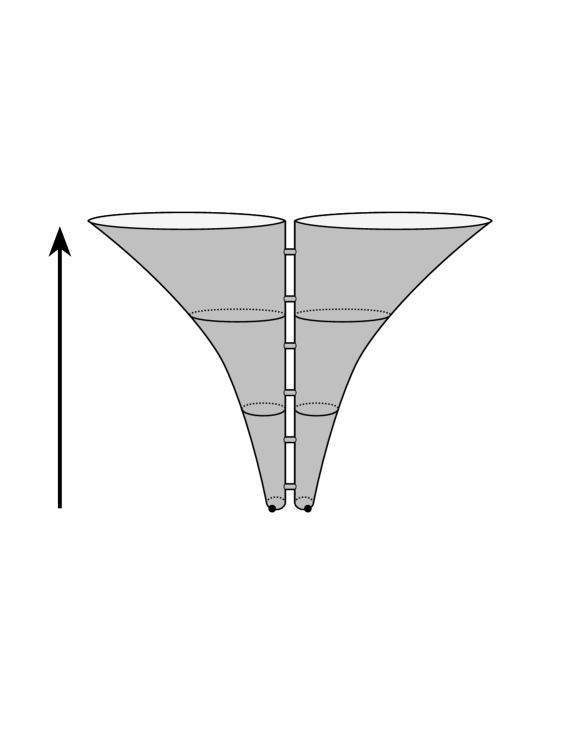
Figure 5.4: Two universes of different flavours 1,2 or 3 knitted together via interaction with flavour 8.

There are a number of aspects of such a knitting procedure which are not yet well understood. The basic process is the one shown in Fig. 2.3, now only with flavours added. Two universes of different flavours 1,2 or 3 propagate in time. Then a “wormhole” of flavour 8 is created and connects them. This wormhole is less than Planckian size. In this way two points in the different universes are connected. This is all fine and everything of this perturbative term (of order $g^{2}G$) can be explicitly calculated, and it corresponds to one of the connections shown in Fig. 5.4. In particular one can from the explicit form of the propagator calculate how the wormhole of flavour 8 glues together two universes of flavour 1 and 2, say. If the wormhole exists for a very short time $\Delta T$, the free energy related to the process is proportional to $1/2\log(L\Delta T)$, where $L$ is the spatial extension of the wormhole. Small wormholes with a short lifetime are thus favoured, as illustrated in Fig. 5.4. However, as indicated in Fig. 5.4 we want this process to be ongoing, such that the two points in the separated universes are identified, and even further, we want such identification for all points in the one-dimensional spaces. This is illustrated in Fig. 5.5 for one-dimensional universes of flavour 1 and 2, say, in this way forming $T^{2}$. Let us label the points in the spatial universe of flavour 1 by coordinate $x^{1}$ and the points in the spatial universe of flavour 2 by coordinate $x^{2}$. All flavour 1 points are now assumed to be connected to all flavour 2 points, and the combined space can be labelled by coordinates $(x^{1},x^{2})$ representing the torus $T^{2}$. It is important in the identification with $T^{2}$ that we have different flavours 1 and 2. The basic wormhole process as shown in Fig.  2.3 also takes place between two spatial universes of the same flavour (as actually shown in Fig. 2.3), but it does not lead to the formation of a space with topology $T^{2}$. Rather, when two points in the different $T^{1}$s are identified it leads to a merging of two $T^{1}$ spaces to a new $T^{1}$ space. This is not possible if the universes have different flavours. In this way the concept of distance appears in the higher dimensional space created by the knitting mechanism.

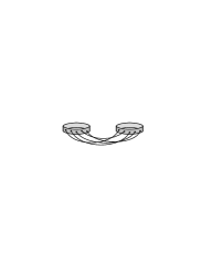
Figure 5.5: Points of two one-dimensional universes with different flavours 1,2 or 3 are identified via knitting, merging the two $T^{1}$ spatial universes into a a two-dimensional $T^{2}$ universe.

Consider now the formation the universe $T^{3}$ from three spatial universes with flavour 1, 2 and 3 mediated by a “wormhole” of flavour 8. The dominant mechanism is shown in Fig. 5.6. The fact that $d_{888}$ is different from 0, as well as $d_{118}$, $d_{228}$ and $d_{338}$, allows for three universes of flavour 8, emerging from spatial universes of flavour 1, 2 and 3, to join in a single point with coupling $d_{888}$. As in the case with only two universes, these interactions are strongest for wormholes of the smallest extension in space and time, and we obtain a gluing between points with three different flavours, labelled by three different coordinates $x^{1}$, $x^{2}$ and $x^{3}$, to a point in $T^{3}$, now labelled by coordinate $(x^{1},x^{2},x^{3})$. The important term mediating knitting is the propagator, related to the kinetic term ${\cal H}_{0}$ in (2.18) and depicted in Fig. 2.3 as a kind of “wormhole” between the two universes. Since the process does not involve the tadpole term in the Hamiltonian we expect the knitting mechanism to respect time reversal invariance.

The situation is the same if we consider the other ${\tilde{H}}_{3}(\leavevmode\raise-0.43057pt\hbox{\twelvemsbm Q})$, $\leavevmode\raise-0.43057pt\hbox{\twelvemsbm Q}=\leavevmode\raise-0.43057pt\hbox{\twelvemsbm R},\leavevmode\raise-0.43057pt\hbox{\twelvemsbm H},\leavevmode\raise-0.43057pt\hbox{\twelvemsbm O}$. In the case of ℝ we have two flavours, 1 and 3, where the universes can expand to infinite spatial volume, while universes with flavour 4,6 and 8 will stay at cut-off scale. For ℍ we five different flavoured universes which can expand to infinity and for 𝕆 we have 9 different flavoured universes which can expand to infinity, where in all cases two universes of the same flavour can merge into a flavour 8 universe which then can split in two universes of one of flavours of potential infinite spatial extension. This follows from the tables of $d_{abc}$ symbols given in Appendix C. Again we conjecture that going beyond the perturbation picture shown in Fig. 2.3, the knitting dynamics operates and creates extended spatial universes of dimensions 2, 3, 5 and 9 for $\leavevmode\raise-0.43057pt\hbox{\twelvemsbm R},\leavevmode\raise-0.43057pt\hbox{\twelvemsbm C},\leavevmode\raise-0.43057pt\hbox{\twelvemsbm H}$ and 𝕆, respectively. If we add the time extension the models we end up with 3, 4, 6 and 10 dimensions of extended spacetime. It is interesting that these are precise the spacetime where classical supersymmetric string theories can be formulated.

Recall that the automorphism groups for the Jordan algebras ${\tilde{H}}_{3}(\leavevmode\raise-0.43057pt\hbox{\twelvemsbm Q})$, $\leavevmode\raise-0.43057pt\hbox{\twelvemsbm Q}=,\leavevmode\raise-0.43057pt\hbox{\twelvemsbm R},\leavevmode\raise-0.43057pt\hbox{\twelvemsbm C},\leavevmode\raise-0.43057pt\hbox{\twelvemsbm H},\leavevmode\raise-0.43057pt\hbox{\twelvemsbm O}$, are $SO(3)$, $SU(3)$, $U\!sp(6)$ and $F_{4}$ and breaking the symmetry in the 8-direction leave us with the unbroken subgroups $SO(2)$, $SO(3)$, $SO(5)$ and $SO(9)$. This picture is compatible with knitting procedure, since the structure constants $d_{aa8}$ are the same in the unbroken directions.

Figure 5.6: Points of three one-dimensional universes with different flavours 1,2 or 3 are identified via knitting, merging the three $T^{1}$ spatial universes into a three-dimensional $T^{3}$ universe.

5.1 A small cosmological constant

The naive perturbative picture we have in our model is that universes of some flavours can be created from nothing with zero spatial extension. They can expand and split into universes of the same or different flavours, and the opposite process where two spatial universes join to one universe is also possible. All these changes are mediated (more or less) by the modes of flavour 8, and our conjecture is that if we consider the flavours which can expand to macroscopic spatial extension in a finite time, they will combine to a higher dimensional space, glued together by the flavour 8 mode. This way of expanding to macroscopic size in a finite time of order $1/\sqrt{-\mu}$ (i.e. in ”Planckian time”) is clearly very different from the standard inflationary expansion, since the model stops to exist for time larger than $1/\sqrt{-\mu}$. However, we believe that that is not really the “end of time” in our model-universe. Wormholes and baby universes are an integral part of our model, and the Coleman mechanism [15] provides a way in which the effective cosmological constant can be very different from the “bare” cosmological constant. Thus it is possible to imagine a scenario where the universes expand very fast, the scale factor growing like

$$a(T)\propto\tan(\sqrt{-\mu}T)$$ (5.1)

rather than the usual exponential growth encountered in a standard inflation scenario, but where the mutual interactions between universes or part of the same universe eventually slows down this expansion before it reaches the strict infinity at a finite time. An effective, modified Friedmann model inspired from CDT was suggested in [14].

6 Discussion and Summary

We have proposed a model for the universe which tries to address the question of which kind of theory could create macroscopic universes starting from “nothing”. “Nothing” in this context is a theory which has no obvious geometric interpretation, but which has the potential to “create” a world with spacetime geometry. The basic idea is very simple and somehow inverting the usual logic of quantum field theory where one starts out with a quadratic non-interacting Hamiltonian and then adds a cubic term which provides the interaction. Here we start with the cubic part as fundamental, and by symmetry breaking we then obtain the quadratic, non-interacting part which allows us to talk about time and space. Motivated by CDT and non-critical string theory we were led to associate the cubic interactions with Jordan algebras. The so-called “magic” Jordan algebras consisting of Hermitian $3\times 3$ matrices with entries being real numbers, complex numbers, quarternions and octonions, respectively, offered the possibility of an interesting symmetry breaking pattern where spacetime with macroscopic extensions could be 3,4 6 and 10 dimensional, can all be derived from the expectation value of the operator

$$\exp\!\bigg{\{}\mbox{res}_{z=0}\Big{(}{\rm tr}{\hskip 1.11206pt}\!:\!\frac{1}{3}J(z)^{3}\!:\!\Big{)}\bigg{\}},$$ (6.2)

where $J(z)=\sum_{\mu}E_{\mu}J^{\mu}(z)$ is a bosonic current in complex plane $z$ with favours $\mu$ and where $E_{\mu}$ are $3\times 3$ Hermitian matrices which belong to one of the “magical” Jordan algebras.

In particular the model based on the traceless part, ${\tilde{H}}_{3}(\leavevmode\raise-0.43057pt\hbox{\twelvemsbm O})$, of the Jordan algebra $H_{3}(\leavevmode\raise-0.43057pt\hbox{\twelvemsbm O})$, where 𝕆 denotes the octonions, is intriguing, since the simplest symmetry breaking pattern leads to 10 extended dimensions and 16 compactified dimensions, very much like the situation present in the heterotic string model. In our models we do not have any concept of supersymmetry, which makes it remarkable that we encounter 3,4,6 and 10 dimensions in the simplest symmetry breaking patterns, since these are precisely the dimensions where classical superstrings can be formulated. Again, this makes the 10 dimensional model especially interesting for the following reason: we know that only the 10 dimensional superstring theory can be consistently quantized. In particular, if one uses lightcone coordinates in the description of the classical string theories, Lorentz invariant is not manifest in the quantized theory, and only in 10 dimensions can it be restored. Also in the CDT quantum gravity models, Lorentz invariance is not manifest. The starting point of the whole construction was precisely a CDT string field theory which was modelled after non-critical lightcone string field theory, and maybe Lorentz invariance can be restored for the model based on the Jordan algebra $H_{3}(\leavevmode\raise-0.43057pt\hbox{\twelvemsbm O})$.

It is also remarkably that a concept like inflation seems to be a natural consequence of our model, although the “inflation” we encounter is somewhat different from the standard inflation. In fact our main problem is to actually stop the universe from expanding to infinity in a finite, very short time. For this we appealed to the Coleman mechanism. In [14] we developed a phenomenological model based on the assumption that the Coleman mechanism would work in our model. The remarkable feature was that still some trace of the creation of baby universes, i.e. the splitting and joining of spatial universes, would survive in our present universe and actually result in an expansion of the universe, very much like what is observed, and this even if the Coleman mechanism had put the cosmological constant to zero. In this way the very origin of our universe gets connected to its eventual destiny. More details of this will be published elsewhere [19], where we will also argue that our model solves the horizon and flatness problem in cosmology and that it makes explicit cosmological predictions which can be verified or falsified in the near future. There are of course many aspects of Coleman’s mechanism which are highly conjectural. One aspect is the concrete existence of wormholes and precisely how they enter in the functional integral and at which scale. Our model is well suited to turn many of these conjectures into concrete calculations, since the starting point from where we were led to the present model, namely CDT string field theory, is a theory of wormholes and not classical wormholes, but fully quantum wormholes. It was precisely constructed to have a mathematical well defined functional integral over geometries with a finite number of wormholes. In the theory outlined in this article the dominant effect of the wormholes is at short distance to glue together one-dimensional spaces with different flavour and create higher dimensional tori and provide toroidal coordinates to these spaces by the knitting mechanism. On the other hand the wormholes can have any length, although long wormholes are less probabilistic favoured, and it is precisely the long wormholes which are used by Coleman. The thickness of these wormholes are of Planck scale in our model and this feature makes the Coleman mechanism much more realistic than some of the attempts to use Einstein-Rosen bridges as the wormholes in the Coleman mechanism. We have not yet managed to perform a detailed calculation leading to a concrete example of the Coleman mechanism, but we believe it is technically doable.

There are many questions which still need to be addressed. It would nice and important to understand precisely which symmetry is present in the model. The $W^{(3)}$ algebra related to the Jordan algebra is only exact at the classical level. Clearly there are some intriguing algebraic relations involving the higher $W^{(n)}$’s, as is clear from the relations reported in Appendices D and E. However, a full understanding is still missing. It is most important to understand in detail the splitting and merging of universes and the process of “knitting”. Perturbatively one can calculate the amplitudes for these processes to any order, but we need a non-perturbative solution to truly understand how higher dimensional space emerges from the one-dimensional spaces of different flavour. If one could understand this, one would also have a tool to discuss the Coleman mechanism in detail, something which to our knowledge never has been done before. Also, it would be highly desirable to have a more explicit realisation of the symmetry breaking mechanism. Here it is postulated and implemented via the choice of a coherent state in the state space defined by the $W^{(3)}$ algebra, but the dynamics behind this is not understood. Of course the challenge is to develop what can be called “dynamics” before space and time have come into existence.

Appendix A Mathematical properties of the Green function

A.1 The eigenvalue equation

Let us consider the following eigenvalue equation obtained in CDT, as described in Sec. 2:

$$H{\hskip 0.55603pt}\psi(L)\,=\,E{\hskip 0.55603pt}\psi(L)\,,$$ (A.1)

where

$$H\,:=\,L\Big{(}\!-\frac{d^{2}}{dL^{2}}+\mu\Big{)}\,,$$ (A.2)

and $E$ is a constant and where the range of $L$ is from 0 to $\infty$. The inner product which makes $H$ an Hermitian operator is

$$\langle\psi^{\prime}|\psi\rangle\,=\,\int_{0}^{\infty}\!\frac{dL}{L}\!\>\psi^{\prime\ast}(L)\psi(L)\,.$$ (A.3)

Changing variable from $L$ to $z$ by

$$z\,:=\,2\sqrt{\mu}\!\;L\,,$$ (A.4)

and also changing the wave function $\psi(L)$ to $\varphi(z)$ by

$$\psi(L)\,=\,z{\hskip 1.11206pt}e^{-z/2}\varphi(z)\,,$$ (A.5)

we obtain

$$\bigg{\{}z\frac{d^{2}}{dz^{2}}+(2-z)\frac{d}{dz}+\frac{E}{2\sqrt{\mu}}-1\bigg{\}}\varphi(z)\,=\,0\,.$$ (A.6)

The general solution of the differential equation (A.6) is

$$\varphi(z)\,=\,c_{1}M\!\!\>\Big{(}1-\frac{E}{2\sqrt{\mu}},2,z\Big{)}\,+\,c_{2}\!\;U\!\!\>\Big{(}1-\frac{E}{2\sqrt{\mu}},2,z\Big{)}\,.$$ (A.7)

$M(\alpha,\beta,z)$ and $U(\alpha,\beta,z)$ are the confluent hypergeometric functions of the first kind and the second kind, respectively. If we demand that $\psi(L)$ is square integrable with respect to the scalar product (A.3) we cannot use the $U$-function and the argument $\alpha=1-E/2\mu$ in $M(\alpha,2,z)$ has to be a non-positive integer $n$. $M(n,2,z)$ is proportional to the associated Laguerre polynomial $L^{1}_{n}(z)$. Recall that the associated Laguerre equation is

$$\bigg{\{}z\frac{d^{2}}{dz^{2}}+(m+1-z)\frac{d}{dz}+n-m\bigg{\}}L^{m}_{n}(z)\,=\,0\,,$$ (A.8)

and the inner product, which makes the differential operator defining $L^{m}_{n}(z)$ Hermitian, is given by

$$\int_{0}^{\infty}\!dz\!\>e^{-z}z^{m}L^{m}_{k}(z)L^{m}_{n}(z)\,=\,\frac{n!}{(n-m)!}\!\;\delta_{k,n}\,,$$ (A.9)

and the completeness is

$$\sum_{n=m}^{\infty}\frac{(n\!-\!m)!}{n!}\!\>L^{m}_{n}(z)L^{m}_{n}(z^{\prime})\,=\,\frac{e^{z}}{z^{m}}\!\;\delta(z-z^{\prime})\,.$$ (A.10)

The definitions of associated Laguerre polynomials are

$$L_{n}^{m}(z)\,:=\,(-1)^{m}\frac{d^{m}}{dz^{m}}\!\>L_{n}(z)\,,$$ (A.12)

$$L_{n}(z)\,:=\,\frac{e^{z}}{n!}\!\;\frac{d^{n}}{dz^{n}}\!\>(\!\>e^{-z}z^{n})\,,\qquad\hbox{[\,$n\!=\!0$, $1$, $2$,\ldots; $m\!=\!0$, $1$, \ldots, $n$\,]}\,.\qquad$$ (A.13)

Therefore, the solution of the above differential equation is

$$\varphi=\varphi_{n}:=\frac{1}{\sqrt{n}}\!\;L^{1}_{n}(z)\,,\qquad E=E_{n}:=2\sqrt{\mu}\,n\,,\qquad\hbox{[\,$n\!=\!1$, $2$, \ldots\,]}\,.\quad$$ (A.14)

Then, we find

$$\psi_{n}(L)\,=\,\frac{A_{n}}{\sqrt{n}}{\hskip 1.11206pt}(2\sqrt{\mu}L){\hskip 1.11206pt}e^{-\sqrt{\mu}L}L^{1}_{n}\big{(}2\sqrt{\mu}\!\;L\big{)}\,,\qquad\quad\hbox{[\,$n\!=\!1$, $2$, \ldots\,]}\,,$$ (A.15)

where $A_{n}$ are the normalization factor. The inner product becomes

$$\langle\psi_{m}|\psi_{n}\rangle\! = \!\int_{0}^{\infty}\!\frac{dL}{L}\!\>\psi^{\ast}_{m}(L)\psi_{n}(L)\ =\ |A_{n}|^{2}{\hskip 0.55603pt}\delta_{m,n}\,,$$ (A.16)

for $m$, $n\geq 1$. So, $A_{n}=1$. On the other hand, the completeness becomes

$$\sum_{n=1}^{\infty}\psi_{n}(L^{\prime})\psi_{n}^{\ast}(L)\! = \!|A_{n}|^{2}{\hskip 1.11206pt}L^{\prime}{\hskip 0.55603pt}\delta(L^{\prime}-L)\,=\,L{\hskip 1.11206pt}\delta(L^{\prime}-L)\,.$$ (A.17)

In the last equation we used $A_{n}\!=\!1$. This result is consistent with the inner product (A.3).

One should note that there exists non-square-integrable solutions. One of them is, for example,

$$\varphi=\varphi_{0}:=\frac{1}{z}\qquad\quad\hskip 40.0ptE=E_{0}:=0\,.$$ (A.18)

Then, the amplitude is

$$\psi_{0}(L)\,=\,A_{0}\!\;e^{-\sqrt{\mu}L}\,.$$ (A.19)

$\psi_{0}(L)$ is not square-integrable and is not orthogonal to other $\psi_{n}(L)$ [ $n\!\geq\!1$ ]. Nevertheless it is an important solution: it is precisely the disk amplitude (2.4), and thus the solution to the Wheeler-deWitt equation for 2d CDT.

A.2 The Green function

By using the formula

$$\sum_{n=m}^{\infty}\frac{z^{n}}{(n\!-\!m\!+\!1)_{m}}\!\>L_{n}^{m}(x)L_{n}^{m}(y)\,=\,\frac{z^{m/2}\,e^{-\,\frac{z}{1-z}(x+y)}}{(1\!-\!z)(xy)^{m/2}}\,I_{m}\!\!\;\bigg{(}\frac{2\sqrt{zxy}}{1\!-\!z}\bigg{)}\,,$$ (A.20)

one finds

$$L{\hskip 0.55603pt}G(L_{0},L;T)\,:=\,\sum_{n=1}^{\infty}e^{-E_{n}T}\psi_{n}(L_{0})\psi_{n}^{\ast}(L)$$

$$=\,\frac{\sqrt{\mu L_{0}L}}{\sinh(\sqrt{\mu}\,T)}\,e^{-\sqrt{\mu}\,(L_{0}+L)\coth(\sqrt{\mu}\,T)}I_{1}\!\!\;\bigg{(}\frac{2\sqrt{\mu L_{0}L}}{\sinh(\sqrt{\mu}\,T)}\bigg{)}\,.$$ (A.21)

For $L_{0}\to 0$ one obtains the amplitude of Big Bang,

$$G_{\rm BB}(L;T)\! := \!\lim_{L_{0}\to 0}\frac{1}{L_{0}}\!\;G(L_{0},L;T)\,=\,\frac{\mu{\hskip 1.11206pt}e^{-\sqrt{\mu}\,L\coth(\sqrt{\mu}\,T)}}{\sinh^{2}(\sqrt{\mu}\,T)}\,.$$ (A.22)

We obtain the disk amplitude (2.4), i.e. a result proportional to $\psi_{0}(L)$, by integrating over $T$.

A.3 The Green function and the average size of space

The expectation value of the length of exit loop is

$$\langle L\rangle_{(L_{0},T)}\,:=\,\frac{\int_{0}^{\infty}dL{\hskip 1.11206pt}L{\hskip 0.55603pt}G(L_{0},L;T)}{\int_{0}^{\infty}dL{\hskip 1.11206pt}G(L_{0},L;T)}\,,$$ (A.23)

where $L_{0}$ is the length of entrance loop. The numerator and the denominator of the right-hand side are

$$\int\limits_{0}^{\infty}\!dL{\hskip 1.11206pt}G(L_{0},L;T)\,=\,\big{(}1-e^{-\sqrt{\mu}\,L_{0}/(\sinh(\sqrt{\mu}\,T)\cosh(\sqrt{\mu}\,T))}\big{)}\,e^{-\sqrt{\mu}\,L_{0}\tanh(\sqrt{\mu}\,T)}\,,$$ (A.24)

$$\int\limits_{0}^{\infty}\!dL{\hskip 1.11206pt}L{\hskip 0.55603pt}G(L_{0},L;T)\,=\,\frac{L_{0}\,e^{-\sqrt{\mu}\,L_{0}\tanh(\sqrt{\mu}\,T)}}{\cosh^{2}(\sqrt{\mu}\,T)}\,,$$ (A.25)

$$\int\limits_{0}^{\infty}\!dL{\hskip 1.11206pt}L^{2}G(L_{0},L;T)\,=\,\bigg{(}\frac{2L_{0}\sinh(\sqrt{\mu}\,T)}{\sqrt{\mu}\,\cosh^{3}(\sqrt{\mu}\,T)}+\frac{L_{0}^{2}}{\cosh^{4}(\sqrt{\mu}\,T)}\bigg{)}\,e^{-\sqrt{\mu}\,L_{0}\tanh(\sqrt{\mu}\,T)}\,.\qquad\quad$$ (A.26)

So, the above average becomes

$$\langle L\rangle_{(L_{0},T)}\! = \!\frac{L_{0}}{\cosh^{2}(\sqrt{\mu}\,T)\big{(}1-e^{-2\sqrt{\mu}\,L_{0}/\sinh(2\sqrt{\mu}\,T)}\big{)}}\,,$$ (A.27)

and the variance $\langle L^{2}\rangle_{(L_{0},T)}-\langle L\rangle^{2}_{(L_{0},T)}$ becomes

$${\rm Var}_{(L_{0},T)}(L)\! = \!\frac{2L_{0}\sinh(\sqrt{\mu}\,T)}{\sqrt{\mu}\cosh^{3}(\sqrt{\mu}\,T)\big{(}1-e^{-2\sqrt{\mu}\,L_{0}/\sinh(2\sqrt{\mu}\,T)}\big{)}}$$ (A.28)

$$\!-\,\frac{L_{0}^{2}\,e^{-2\sqrt{\mu}\,L_{0}/\sinh(2\sqrt{\mu}\,T)}}{\cosh^{4}(\sqrt{\mu}\,T)\big{(}1-e^{-2\sqrt{\mu}\,L_{0}/\sinh(2\sqrt{\mu}\,T)}\big{)}^{2}}\,.$$

For $L_{0}\!=\!0$, we obtain

$$\langle L\rangle_{T}=\frac{1}{\sqrt{\mu}}\,\tanh\sqrt{\mu}T,\qquad{\rm Var}_{T}(L)=\frac{1}{\mu}\,\tanh^{2}\sqrt{\mu}T=\langle L\rangle^{2}_{T}$$ (A.29)

$\langle L\rangle_{T}$ is the average size of space at time $T$ after the Big Bang, as already mentioned in the main text, (2.8). Already after a time not much longer that $T\sim 1/\sqrt{\mu}$ the size of space has almost reached its maximum $L_{\rm cs}:=\frac{1}{\sqrt{\mu}}$. It should also be noted that the standard deviation $\Delta L(T)=\sqrt{{\rm Var}_{T}(L)}=\langle L\rangle_{T}$. So the standard deviation is quite large.

If the spatial extent of the universe shrinks to zero, it will cease to exist and be absorbed in the vacuum. The probability that this happens at time $T$, starting out with the Big Bang, is proportional to

$$\lim_{L_{0}\to 0}\lim_{L\to 0}\frac{1}{L_{0}}{\hskip 1.11206pt}G(L_{0},L;T)\,=\,\frac{\mu}{\sinh^{2}(\sqrt{\mu}\,T)}\,.$$ (A.30)

A.4 The Green function with negative cosmological constant

The differential equation (A.1) is analytic with respect to the coefficient $\mu$. Without explicit calculation one can make the analytic continuation $\mu\to e^{i\theta}\mu$ [ $0\!\leq\!\theta\!\leq\!\pi$ ] in the solutions which we already obtained.

When $\mu$ is negative, the Green function (A.2) becomes

$$L{\hskip 0.55603pt}G(L_{0},L;T)\,=\,\frac{\sqrt{-\mu L_{0}L}}{\sin(\sqrt{-\mu}\,T)}\,e^{-\sqrt{-\mu}\,(L_{0}+L)\cot(\sqrt{-\mu}\,T)}I_{1}\!\!\;\bigg{(}\frac{2\sqrt{-\mu L_{0}L}}{\sin(\sqrt{-\mu}\,T)}\bigg{)}\,,$$

and the Big Bang amplitude (A.22) also becomes

$$G_{\rm BB}(L;T)\! = \!\frac{-\mu{\hskip 1.11206pt}e^{-\sqrt{-\mu}\,L\cot(\sqrt{-\mu}\,T)}}{\sin^{2}(\sqrt{-\mu}\,T)}\,.$$ (A.32)

When $\mu$ is negative, the average length of the exit loop when we start at $L_{0}=0$, becomes

$$\langle L\rangle_{T}=\frac{1}{\sqrt{-\mu}}\,\tan\sqrt{-\mu}\,T\,.$$ (A.33)

The average length goes to infinity for When $T\to T_{\rm ps}:=\frac{\pi}{2\sqrt{-\mu}}$. Thus we have a kind of inflation, culminating at $T_{\rm ps}$ where this is an infinitely fast expansion. The “inflation” can be seen from (A.32), too. When $T$ is less than $T_{\rm ps}$, $L_{\rm max}$, the peak of $G_{\rm bb}(L;T)$ with fixed $T$, is finite. But, when $T$ approaches $T_{\rm ps}$, $L_{\rm max}$ goes to infinity.

When $\mu$ is negative, the probability that a Big Bang universe disappears at time $T<T_{\rm ps}$becomes

$$\lim_{L_{0}\to 0}\lim_{L\to 0}\frac{1}{L_{0}}{\hskip 1.11206pt}G(L_{0},L;T)\,=\,\frac{-\mu}{\sin^{2}(\sqrt{-\mu}\,T)}\,.$$ (A.34)

A.5 The Green function without cosmological constant

We can directly take the limit $\mu=0$ in the above expressions and obtain the results for zero cosmological constant. When $\mu$ is zero, the Green function (A.2) becomes

$$L{\hskip 0.55603pt}G(L_{0},L;T)\,=\,\frac{\sqrt{L_{0}L}}{T}\,e^{-(L_{0}+L)/T}I_{1}\!\!\;\bigg{(}\frac{2\sqrt{L_{0}L}}{T}\bigg{)}\,,$$ (A.35)

and the Big Bang amplitude (A.22) also becomes

$$G_{\rm BB}(L;T)\! = \!\frac{e^{-L/T}}{T^{2}}\,.$$ (A.36)

Instead of (A.29) we have

$$\langle L\rangle_{T}=\frac{1}{\sqrt{\mu}}\,\tanh\sqrt{\mu}T,\qquad{\rm Var}_{T}(L)=\frac{1}{\mu}\,\tanh^{2}\sqrt{\mu}T=\langle L\rangle^{2}_{T}$$ (A.37)

and instead of (A.30)

$$\lim_{L_{0}\to 0}\lim_{L\to 0}\frac{1}{L_{0}}{\hskip 1.11206pt}G(L_{0},L;T)\,=\,\frac{1}{T^{2}}\,.$$ (A.38)

Appendix B Real, complex, quaternion and octonion numbers

The set of real numbers, complex numbers, quaternions, octonions is denoted by ℝ, ℂ, ℍ, 𝕆, respectively. One of real numbers, complex numbers, quaternions, octonions is

$$x\,+\sum_{n}e_{n}x_{n}\,,$$ (B.39)

where $x$, $x_{1}$, $x_{2}$, …are real numbers, and the set of $e_{n}$, i.e. $E=\{e_{1},e_{2},\ldots\}$ is

$$E\ \stackrel{{\scriptstyle\rm def}}{{\equiv}}\ \{\,\,\} \hbox{[\,for $\leavevmode\raise-0.43057pt\hbox{\twelvemsbm R}$\,]}\,,$$ (B.40)

$$E\ \stackrel{{\scriptstyle\rm def}}{{\equiv}}\ \{\,i\,\} \hbox{[\,for $\leavevmode\raise-0.43057pt\hbox{\twelvemsbm C}$\,]}\,,$$ (B.41)

$$E\ \stackrel{{\scriptstyle\rm def}}{{\equiv}}\ \{\,i,\,j,\,k\,\} \hbox{[\,for $\leavevmode\raise-0.43057pt\hbox{\twelvemsbm H}$\,]}\,,$$ (B.42)

$$E\ \stackrel{{\scriptstyle\rm def}}{{\equiv}}\ \{\,i,\,j,\,k,\,\ell,\,\bar{i},\,\bar{j},\,\bar{k}\,\} \hbox{[\,for $\leavevmode\raise-0.43057pt\hbox{\twelvemsbm O}$\,]}\,.$$ (B.43)

The number of imaginary units, i.e. $|E{\hskip 0.55603pt}|$, is $0$, $1$, $3$, $7$, for ℝ, ℂ, ℍ, 𝕆, respectively. For real numbers, (B.39) reads $x$ [ $x{}\in{}\leavevmode\raise-0.43057pt\hbox{\twelvemsbm R}$ ]. For complex numbers, (B.39) reads $x{}+{}iy$ [ $x$, $y{}\in{}\leavevmode\raise-0.43057pt\hbox{\twelvemsbm R}$ ]. For quaternions and octonions, we will explain the details in the following sections.

B.1 Quaternions

According to (B.39) and (B.42), the quaternions are numbers defined by

$$z\ =\ x{\hskip 0.55603pt}+{\hskip 0.55603pt}i{\hskip 0.55603pt}y{\hskip 0.55603pt}+{\hskip 0.55603pt}j{\hskip 0.55603pt}u{\hskip 0.55603pt}+{\hskip 0.55603pt}k{\hskip 0.55603pt}v\qquad\quad\hbox{[\,$x$, $y$, $u$, $v{}\in{}\leavevmode\raise-0.43057pt\hbox{\twelvemsbm R}$\,]}$$ (B.44)

The quaternion conjugate of $z$ is defined by

$$z^{\ast}\ \stackrel{{\scriptstyle\rm def}}{{\equiv}}\ x{\hskip 0.55603pt}-{\hskip 0.55603pt}i{\hskip 0.55603pt}y{\hskip 0.55603pt}-{\hskip 0.55603pt}j{\hskip 0.55603pt}u{\hskip 0.55603pt}-{\hskip 0.55603pt}k{\hskip 0.55603pt}v\,.$$ (B.45)

The norm of a quaternion is defined by

$$|z|\ \stackrel{{\scriptstyle\rm def}}{{\equiv}}\ \sqrt{x^{2}+y^{2}+u^{2}+v^{2}}\,.$$ (B.46)

The multiplication of these imaginary units are as follows:

$$i^{2}\,=\,j^{2}\,=\,k^{2}\,=\,ijk\,=\,-1$$

$$i{\hskip 0.55603pt}j\,=\,-j{\hskip 0.55603pt}i\,=\,k\qquad j{\hskip 0.55603pt}k\,=\,-k{\hskip 0.55603pt}j\,=\,i\qquad k{\hskip 0.55603pt}i\,=\,-i{\hskip 0.55603pt}k\,=\,j$$ (B.47)

Multiplications of quaternions do not necessarily do not necessarily commute, but satisfy associativity.

B.2 Octonions

According to (B.39) and (B.43), the octonions are numbers defined by

$$z\! = \!x{\hskip 1.11206pt}+{\hskip 1.11206pt}i{\hskip 0.27802pt}y{\hskip 1.11206pt}+{\hskip 1.11206pt}j{\hskip 0.27802pt}u{\hskip 1.11206pt}+{\hskip 1.11206pt}k{\hskip 0.27802pt}v{\hskip 1.11206pt}+{\hskip 1.11206pt}\ell{\hskip 0.55603pt}\bar{x}{\hskip 1.11206pt}+{\hskip 1.11206pt}\bar{i}{\hskip 0.55603pt}\bar{y}{\hskip 1.11206pt}+{\hskip 1.11206pt}\bar{j}{\hskip 0.55603pt}\bar{u}{\hskip 1.11206pt}+{\hskip 1.11206pt}\bar{k}{\hskip 0.55603pt}\bar{v}$$ (B.48)

$$= \!\xi{}+{}\eta{\hskip 0.55603pt}\ell$$

where $x$, $y$, $u$, $v$, $\bar{x}$, $\bar{y}$, $\bar{u}$, $\bar{v}{}\in{}\leavevmode\raise-0.43057pt\hbox{\twelvemsbm R}$, and

$$\xi\! = \!x{\hskip 1.11206pt}+{\hskip 1.11206pt}i{\hskip 0.27802pt}y{\hskip 1.11206pt}+{\hskip 1.11206pt}j{\hskip 0.27802pt}u{\hskip 1.11206pt}+{\hskip 1.11206pt}k{\hskip 0.27802pt}v\in\leavevmode\raise-0.43057pt\hbox{\twelvemsbm H}$$

$$\eta\! = \!\bar{x}{\hskip 1.11206pt}+{\hskip 1.11206pt}i{\hskip 0.27802pt}\bar{y}{\hskip 1.11206pt}+{\hskip 1.11206pt}j{\hskip 0.27802pt}\bar{u}{\hskip 1.11206pt}+{\hskip 1.11206pt}k{\hskip 0.27802pt}\bar{v}\in\leavevmode\raise-0.43057pt\hbox{\twelvemsbm H}$$ (B.49)

The octonion conjugate of $z$ is defined by

$$z^{\ast}\! \stackrel{{\scriptstyle\rm def}}{{\equiv}} \!x{\hskip 0.55603pt}-{\hskip 0.55603pt}i{\hskip 0.55603pt}y{\hskip 0.55603pt}-{\hskip 0.55603pt}j{\hskip 0.55603pt}u{\hskip 0.55603pt}-{\hskip 0.55603pt}k{\hskip 0.55603pt}v{\hskip 0.55603pt}-{\hskip 0.55603pt}\ell{\hskip 0.55603pt}\bar{x}{\hskip 0.55603pt}-{\hskip 0.55603pt}\bar{i}{\hskip 0.55603pt}\bar{y}{\hskip 0.55603pt}-{\hskip 0.55603pt}\bar{j}{\hskip 0.55603pt}\bar{u}{\hskip 0.55603pt}-{\hskip 0.55603pt}\bar{k}{\hskip 0.55603pt}\bar{v}$$ (B.50)

$$= \!\xi^{\ast}{}-{}\eta{\hskip 0.55603pt}\ell$$

The norm of a octonion is defined by

$$|z|\! \stackrel{{\scriptstyle\rm def}}{{\equiv}} \!\sqrt{x^{2}+y^{2}+u^{2}+v^{2}+\bar{x}^{2}+\bar{y}^{2}+\bar{u}^{2}+\bar{v}^{2}}$$ (B.51)

$$= \!\sqrt{|\xi|^{2}+|\eta|^{2}}$$

The multiplication of two octonions is defined by

$$(\xi{}+{}\eta{\hskip 0.55603pt}\ell{\hskip 0.55603pt})(\xi^{\prime}{}+{}\eta^{\prime}{}\ell{\hskip 0.55603pt})\ =\ \xi\xi^{\prime}{}-{}\eta^{\prime\ast}\eta+(\eta^{\prime}\xi{}+{}\eta{\hskip 0.55603pt}\xi^{\prime\ast}){\hskip 0.83405pt}\ell$$ (B.52)

where $\xi$, $\eta$, $\xi^{\prime}$, $\eta^{\prime}$ are quaternions. The squares of imaginary units are all $-1$, and all imaginary units anticommute, in the same way as the imaginary units of quaternions do. So multiplication is not necessarily commutative, but also it is not necessarily associative.

Appendix C Symmetric and Hermitian Matrices

Let us consider the set of $K{}\times{}K$ Hemitian matrices. We classify the Hermitian matrices into four group, where the matrix elements are real, complex, quaternion, octonion, respectively. Hermiticity means that matrix elements satisfy $a_{ij}=a^{*}_{ji}$, where conjugation $a^{*}$ is defined above (in the non-trial cases of quarternions and octonions).

The real vectorspace of these Hermitian matrices is a direct sum of the one-dimensional vector space spanned by the unit matrix and the vector space spanned by the traceless Hermitian matrices. We denote a basis of the traceless Hermitian matrices by $\{\lambda_{a}|\,\hbox{$a\!=\!1$, \ldots, $N$}\}$. For the traceless matrices we can write $S+E\!\times A$, where $S$ is the set of real symmetric traceless matrices, $A$ is the set of real antisymmetric matrices, $E$ is the set of imaginary units defined in eqs. (B.40)-(B.43). The number of real symmetric traceless matrices is $|S|{}={}\frac{K(K+1)}{2}{}-{}1$, and the number of real antisymmetric matrices is $|A|{}={}\frac{K(K-1)}{2}$. $E\!\times\!A$ is the set which consists of all possible multiplications of an element of $E$ and an element of $A$, so $|E\!\times\!A|=|E|\!\cdot\!|A|$. Let $N$ denote the dimension of the set $S+E\!\times\!A$. Thus

$$N\,=\,|S+E\!\times\!A|\,=\,|S|{}+{}|E|\!\cdot\!|A|$$ (C.53)

C.1 $2$D Hermitian-matrix type

In the case of $2{}\times{}2$ matrices, the set of symmetric traceless matices is $S\!\stackrel{{\scriptstyle\rm def}}{{\equiv}}\!\{S_{xy},S_{z}\}$, where

$$S_{xy}\stackrel{{\scriptstyle\rm def}}{{\equiv}}\left(\!\begin{array}[]{cc}0&1\\ 1&0\\ \end{array}\!\right)\,,\qquad S_{z}\stackrel{{\scriptstyle\rm def}}{{\equiv}}\left(\!\begin{array}[]{cc}1&0\\ 0&-1\\ \end{array}\!\right)\,,$$ (C.58)

and the set of antisymmetric matices is $A\!\stackrel{{\scriptstyle\rm def}}{{\equiv}}\!\{A_{xy}\}$, where

$$A_{xy}\stackrel{{\scriptstyle\rm def}}{{\equiv}}\left(\!\begin{array}[]{cc}0&-1\\ 1&0\\ \end{array}\!\right)\,.$$ (C.61)

Since $|S|\!=\!2$, $|A|\!=\!1$ in the case of $K\!=\!2$, $N\!=\!2$, $3$, $5$, $9$, for ℝ, ℂ, ℍ, 𝕆 matrix types, respectively. The concrete definitions are listed in the following subsections.

C.1.1 Real symmetric traceless matrices

$$\lambda_{1}=S_{xy}\,,\qquad\lambda_{3}=S_{z}\,.$$ (C.62)

C.1.2 Hermite traceless matrices

$$\lambda_{1}=S_{xy}\,,\qquad\lambda_{3}=S_{z}\,,\qquad\lambda_{2}=iA_{xy}\,.$$ (C.63)

In this case, $\lambda_{a}$ are the Pauli matrices.

C.1.3 Quaternion Hermite traceless matrices

$$\lambda_{1}=S_{xy}\,,\qquad\lambda_{3}=S_{z}\,,\qquad\lambda_{2}=iA_{xy}\,,\qquad\lambda_{2^{\prime}}=jA_{xy}\,,\qquad\lambda_{2^{\prime\prime}}=kA_{xy}\,.\qquad$$ (C.64)

C.1.4 Octonion Hermite traceless matrices

$$\lambda_{1}=S_{xy}\,,\qquad\lambda_{3}=S_{z}\,,\qquad\lambda_{2}=iA_{xy}\,,\qquad\lambda_{2^{\prime}}=jA_{xy}\,,\qquad\lambda_{2^{\prime\prime}}=kA_{xy}\,,\qquad$$

$$\lambda_{2^{\circ}}=\ell A_{xy}\,,\qquad\lambda_{\bar{2}}=\bar{i}A_{xy}\,,\qquad\lambda_{\bar{2}^{\prime}}=\bar{j}A_{xy}\,,\qquad\lambda_{\bar{2}^{\prime\prime}}=\bar{k}A_{xy}\,.\qquad$$ (C.65)

C.2 $3$D Hermitian-matrix type

In the case of $3{}\times{}3$ matrices, the set of symmetric traceless matices is

$$S\,\stackrel{{\scriptstyle\rm def}}{{\equiv}}\,\{S_{xy},\,S_{yz},\,S_{zx},\,S_{x^{2}-y^{2}},\,S_{z^{2}}\}\,,$$ (C.66)

where

$$S_{xy}\stackrel{{\scriptstyle\rm def}}{{\equiv}}\left(\!\begin{array}[]{ccc}0&1&0\\ 1&0&0\\ 0&0&0\end{array}\!\right)\,,\quad S_{yz}\stackrel{{\scriptstyle\rm def}}{{\equiv}}\left(\!\begin{array}[]{ccc}0&0&0\\ 0&0&1\\ 0&1&0\end{array}\!\right)\,,\quad S_{zx}\stackrel{{\scriptstyle\rm def}}{{\equiv}}\left(\!\begin{array}[]{ccc}0&0&1\\ 0&0&0\\ 1&0&0\end{array}\!\right)\,,$$ (C.76)

$$S_{x^{2}-y^{2}}\stackrel{{\scriptstyle\rm def}}{{\equiv}}\left(\!\begin{array}[]{ccc}1&0&0\\ 0&-1&0\\ 0&0&0\end{array}\!\right)\,,\quad S_{z^{2}}\stackrel{{\scriptstyle\rm def}}{{\equiv}}\frac{1}{\sqrt{3}}\!\left(\!\begin{array}[]{ccc}1&0&0\\ 0&1&0\\ 0&0&-2\end{array}\!\right)\,,\qquad\$$ (C.83)

and the set of antisymmetric matices is

$$A\,\stackrel{{\scriptstyle\rm def}}{{\equiv}}\,\{A_{xy},A_{yz},A_{zx}\}\,,$$ (C.84)

where

$$A_{xy}\stackrel{{\scriptstyle\rm def}}{{\equiv}}\left(\!\begin{array}[]{ccc}0&-1&0\\ 1&0&0\\ 0&0&0\end{array}\!\right)\,,\quad A_{yz}\stackrel{{\scriptstyle\rm def}}{{\equiv}}\left(\!\begin{array}[]{ccc}0&0&0\\ 0&0&-1\\ 0&1&0\end{array}\!\right)\,,\quad A_{zx}\stackrel{{\scriptstyle\rm def}}{{\equiv}}\left(\!\begin{array}[]{ccc}0&0&1\\ 0&0&0\\ -1&0&0\end{array}\!\right)\,.\qquad\$$ (C.94)

Since $|S|\!=\!5$, $|A|\!=\!3$ in the case of $K\!=\!3$, $N\!=\!5$, $8$, $14$, $26$, for ℝ, ℂ, ℍ, 𝕆 matrix types, respectively. The concrete definitions are listed in the following subsections.

C.2.1 Real symmetric traceless matrices

$$\lambda_{1}=S_{xy}\,,\qquad\lambda_{6}=S_{yz}\,,\qquad\lambda_{4}=S_{zx}\,,\qquad\lambda_{3}=S_{x^{2}-y^{2}}\,,\qquad\lambda_{8}=S_{z^{2}}\,.\qquad$$ (C.95)

The non-zero $d_{abc}$ [ $a$, $b$, $c\!=\!1$, … ] are in the following:

$$d_{118}\,=\,d_{338}\,=\,\frac{1}{\sqrt{3}}\,,\qquad d_{448}\,=\,d_{668}\,=\,-{\hskip 1.11206pt}\frac{1}{2\sqrt{3}}\,,$$

$$d_{888}\,=\,-{\hskip 1.11206pt}\frac{1}{\sqrt{3}}\,,\qquad d_{344}\,=\,\frac{1}{2}\,,\qquad\quad d_{366}\,=\,-{\hskip 1.11206pt}\frac{1}{2}\,,\qquad\quad d_{146}\,=\,\frac{1}{2}\,.\qquad$$ (C.96)

We here omit $d_{abc}$ obtained by the permutation of $a$, $b$, $c$.

C.2.2 Hermite traceless matrices

$$\lambda_{1}=S_{xy}\,,\qquad\lambda_{6}=S_{yz}\,,\qquad\lambda_{4}=S_{zx}\,,\qquad\lambda_{3}=S_{x^{2}-y^{2}}\,,\qquad\lambda_{8}=S_{z^{2}}\,,\qquad$$

$$\lambda_{2}=iA_{xy}\,,\qquad\lambda_{7}=iA_{yz}\,,\qquad\lambda_{5}=-iA_{zx}\,.$$ (C.97)

In this case, $\lambda_{a}$ are the Gell-Mann matrices. The non-zero $d_{abc}$ [ $a$, $b$, $c\!=\!1$, … ] are in the following:

$$d_{118}\,=\,d_{228}\,=\,d_{338}\,=\,\frac{1}{\sqrt{3}}\,,\qquad d_{448}\,=\,d_{558}\,=\,d_{668}\,=\,d_{778}\,=\,-{\hskip 1.11206pt}\frac{1}{2\sqrt{3}}\,,$$

$$d_{888}\,=\,-{\hskip 1.11206pt}\frac{1}{\sqrt{3}}\,,\qquad d_{344}\,=\,d_{355}\,=\,\frac{1}{2}\,,\qquad\quad d_{366}\,=\,d_{377}\,=\,-{\hskip 1.11206pt}\frac{1}{2}\,,$$

$$d_{146}\,=\,d_{157}\,=\,d_{256}\,=\,\frac{1}{2}\,,\qquad\quad d_{247}\,=\,-{\hskip 1.11206pt}\frac{1}{2}\,.$$ (C.98)

Again we here omit $d_{abc}$ obtained by the permutation of $a$, $b$, $c$.

C.2.3 Quaternion Hermite traceless matrices

$$\lambda_{1}=S_{xy}\,,\qquad\lambda_{6}=S_{yz}\,,\qquad\lambda_{4}=S_{zx}\,,\qquad\lambda_{3}=S_{x^{2}-y^{2}}\,,\qquad\lambda_{8}=S_{z^{2}}\,,\qquad$$

$$\lambda_{2}=iA_{xy}\,,\qquad\lambda_{7}=iA_{yz}\,,\qquad\lambda_{5}=-iA_{zx}\,,\qquad$$

$$\lambda_{2^{\prime}}=jA_{xy}\,,\qquad\lambda_{7^{\prime}}=jA_{yz}\,,\qquad\lambda_{5^{\prime}}=-jA_{zx}\,,\qquad$$

$$\lambda_{2^{\prime\prime}}=kA_{xy}\,,\qquad\lambda_{7^{\prime\prime}}=kA_{yz}\,,\qquad\lambda_{5^{\prime\prime}}=-kA_{zx}\,.$$ (C.99)

Non-zero $d_{abc}$ [ $a$, $b$, $c\!=\!1$, … ] are in the following:

$$d_{118}\,=\,d_{228}\,=\,d_{2^{\prime}2^{\prime}8}\,=\,d_{2^{\prime\prime}2^{\prime\prime}8}\,=\,d_{338}\,=\,\frac{1}{\sqrt{3}}\,,$$ (C.100)

$$d_{448}\,=\,d_{558}\,=\,d_{5^{\prime}5^{\prime}8}\,=\,d_{5^{\prime\prime}5^{\prime\prime}8}\,=\,d_{668}\,=\,d_{778}\,=\,d_{7^{\prime}7^{\prime}8}\,=\,d_{7^{\prime\prime}7^{\prime\prime}8}\,=\,-{\hskip 1.11206pt}\frac{1}{2\sqrt{3}}\,,$$

$$d_{888}\,=\,-{\hskip 1.11206pt}\frac{1}{\sqrt{3}}\,,$$

$$d_{344}\,=\,d_{355}\,=\,d_{35^{\prime}5^{\prime}}\,=\,d_{35^{\prime\prime}5^{\prime\prime}}\,=\,\frac{1}{2}\,,$$

$$d_{366}\,=\,d_{377}\,=\,d_{37^{\prime}7^{\prime}}\,=\,d_{37^{\prime\prime}7^{\prime\prime}}\,=\,-{\hskip 1.11206pt}\frac{1}{2}\,,$$

$$d_{146}\,=\,d_{157}\,=\,d_{15^{\prime}7^{\prime}}\,=\,d_{15^{\prime\prime}7^{\prime\prime}}\,=\,d_{256}\,=\,d_{2^{\prime}5^{\prime}6}\,=\,d_{2^{\prime\prime}5^{\prime\prime}6}\,=\,\frac{1}{2}\,,$$

$$d_{247}\,=\,d_{2^{\prime}47^{\prime}}\,=\,d_{2^{\prime\prime}47^{\prime\prime}}\,=\,-{\hskip 1.11206pt}\frac{1}{2}\,,$$

$$d_{25^{\prime}7^{\prime\prime}}\,=\,d_{2^{\prime}5^{\prime\prime}7}\,=\,d_{2^{\prime\prime}57^{\prime}}\,=\,\frac{1}{2}\,,\qquad\quad d_{2^{\prime}57^{\prime\prime}}\,=\,d_{2^{\prime\prime}5^{\prime}7}\,=\,d_{25^{\prime\prime}7^{\prime}}\,=\,-{\hskip 1.11206pt}\frac{1}{2}\,.$$

Also here we here omit $d_{abc}$ obtained by the permutation of $a$, $b$, $c$.

C.2.4 Octonion Hermite traceless matrices

$$\lambda_{1}=S_{xy}\,,\qquad\lambda_{6}=S_{yz}\,,\qquad\lambda_{4}=S_{zx}\,,\qquad\lambda_{3}=S_{x^{2}-y^{2}}\,,\qquad\lambda_{8}=S_{z^{2}}\,,\qquad$$

$$\lambda_{2}=iA_{xy}\,,\qquad\lambda_{7}=iA_{yz}\,,\qquad\lambda_{5}=-iA_{zx}\,,\qquad$$

$$\lambda_{2^{\prime}}=jA_{xy}\,,\qquad\lambda_{7^{\prime}}=jA_{yz}\,,\qquad\lambda_{5^{\prime}}=-jA_{zx}\,,\qquad$$

$$\lambda_{2^{\prime\prime}}=kA_{xy}\,,\qquad\lambda_{7^{\prime\prime}}=kA_{yz}\,,\qquad\lambda_{5^{\prime\prime}}=-kA_{zx}\,,\qquad$$

$$\lambda_{2^{\circ}}=\ell A_{xy}\,,\qquad\lambda_{7^{\circ}}=\ell A_{yz}\,,\qquad\lambda_{5^{\circ}}=-\ell A_{zx}\,,\qquad$$

$$\lambda_{\bar{2}}=\bar{i}A_{xy}\,,\qquad\lambda_{\bar{7}}=\bar{i}A_{yz}\,,\qquad\lambda_{\bar{5}}=-\bar{i}A_{zx}\,,\qquad$$

$$\lambda_{\bar{2}^{\prime}}=\bar{j}A_{xy}\,,\qquad\lambda_{\bar{7}^{\prime}}=\bar{j}A_{yz}\,,\qquad\lambda_{\bar{5}^{\prime}}=-\bar{j}A_{zx}\,,\qquad$$

$$\lambda_{\bar{2}^{\prime\prime}}=\bar{k}A_{xy}\,,\qquad\lambda_{\bar{7}^{\prime\prime}}=\bar{k}A_{yz}\,,\qquad\lambda_{\bar{5}^{\prime\prime}}=-\bar{k}A_{zx}\,.$$ (C.101)

The non-zero $d_{abc}$ [ $a$, $b$, $c\!=\!1$, … ] are in the following:

$$d_{118}\,=\,d_{228}\,=\,d_{2^{\prime}2^{\prime}8}\,=\,d_{2^{\prime\prime}2^{\prime\prime}8}\,=\,d_{2^{\circ}2^{\circ}8}\,=\,d_{\bar{2}\bar{2}8}\,=\,d_{\bar{2}^{\prime}\bar{2}^{\prime}8}\,=\,d_{\bar{2}^{\prime\prime}\bar{2}^{\prime\prime}8}\,=\,d_{338}\,=\,\frac{1}{\sqrt{3}}\,,$$

$$d_{448}\,=\,d_{558}\,=\,d_{5^{\prime}5^{\prime}8}\,=\,d_{5^{\prime\prime}5^{\prime\prime}8}\,=\,d_{5^{\circ}5^{\circ}8}\,=\,d_{\bar{5}\bar{5}8}\,=\,d_{\bar{5}^{\prime}\bar{5}^{\prime}8}\,=\,d_{\bar{5}^{\prime\prime}\bar{5}^{\prime\prime}8}\,=\,$$

$$d_{668}\,=\,d_{778}\,=\,d_{7^{\prime}7^{\prime}8}\,=\,d_{7^{\prime\prime}7^{\prime\prime}8}\,=\,d_{7^{\circ}7^{\circ}8}\,=\,d_{\bar{7}\bar{7}8}\,=\,d_{\bar{7}^{\prime}\bar{7}^{\prime}8}\,=\,d_{\bar{7}^{\prime\prime}\bar{7}^{\prime\prime}8}\,=\,-{\hskip 1.11206pt}\frac{1}{2\sqrt{3}}\,,$$

$$d_{888}\,=\,-{\hskip 1.11206pt}\frac{1}{\sqrt{3}}\,,$$

$$d_{344}\,=\,d_{355}\,=\,d_{35^{\prime}5^{\prime}}\,=\,d_{35^{\prime\prime}5^{\prime\prime}}\,=\,d_{35^{\circ}5^{\circ}}\,=\,d_{3\bar{5}\bar{5}}\,=\,d_{3\bar{5}^{\prime}\bar{5}^{\prime}}\,=\,d_{3\bar{5}^{\prime\prime}\bar{5}^{\prime\prime}}\,=\,\frac{1}{2}\,,$$

$$d_{366}\,=\,d_{377}\,=\,d_{37^{\prime}7^{\prime}}\,=\,d_{37^{\prime\prime}7^{\prime\prime}}\,=\,d_{37^{\circ}7^{\circ}}\,=\,d_{3\bar{7}\bar{7}}\,=\,d_{3\bar{7}^{\prime}\bar{7}^{\prime}}\,=\,d_{3\bar{7}^{\prime\prime}\bar{7}^{\prime\prime}}\,=\,-{\hskip 1.11206pt}\frac{1}{2}\,,$$

$$d_{146}\,=\,d_{157}\,=\,d_{15^{\prime}7^{\prime}}\,=\,d_{15^{\prime\prime}7^{\prime\prime}}\,=\,d_{15^{\circ}7^{\circ}}\,=\,d_{1\bar{5}\bar{7}}\,=\,d_{1\bar{5}^{\prime}\bar{7}^{\prime}}\,=\,d_{1\bar{5}^{\prime\prime}\bar{7}^{\prime\prime}}\,=\,$$

$$d_{256}\,=\,d_{2^{\prime}5^{\prime}6}\,=\,d_{2^{\prime\prime}5^{\prime\prime}6}\,=\,d_{2^{\circ}5^{\circ}6}\,=\,d_{\bar{2}\bar{5}6}\,=\,d_{\bar{2}^{\prime}\bar{5}^{\prime}6}\,=\,d_{\bar{2}^{\prime\prime}\bar{5}^{\prime\prime}6}\,=\,\frac{1}{2}\,,$$

$$d_{247}\,=\,d_{2^{\prime}47^{\prime}}\,=\,d_{2^{\prime\prime}47^{\prime\prime}}\,=\,d_{2^{\circ}47^{\circ}}\,=\,d_{\bar{2}4\bar{7}}\,=\,d_{\bar{2}^{\prime}4\bar{7}^{\prime}}\,=\,d_{\bar{2}^{\prime\prime}4\bar{7}^{\prime\prime}}\,=\,-{\hskip 1.11206pt}\frac{1}{2}\,,$$

$$d_{25^{\prime}7^{\prime\prime}}\,=\,d_{2^{\prime}5^{\prime\prime}7}\,=\,d_{2^{\prime\prime}57^{\prime}}\,=\,d_{\bar{2}^{\prime}\bar{5}7^{\prime\prime}}\,=\,d_{\bar{2}^{\prime\prime}\bar{5}^{\prime}7}\,=\,d_{\bar{2}\bar{5}^{\prime\prime}7^{\prime}}\,=\,$$

$$d_{\bar{2}^{\prime}5\bar{7}^{\prime\prime}}\,=\,d_{\bar{2}^{\prime\prime}5^{\prime}\bar{7}}\,=\,d_{\bar{2}5^{\prime\prime}\bar{7}^{\prime}}\,=\,d_{2^{\prime}\bar{5}\bar{7}^{\prime\prime}}\,=\,d_{2^{\prime\prime}\bar{5}^{\prime}\bar{7}}\,=\,d_{2\bar{5}^{\prime\prime}\bar{7}^{\prime}}\,=\,$$

$$d_{\bar{2}57^{\circ}}\,=\,d_{\bar{2}^{\prime}5^{\prime}7^{\circ}}\,=\,d_{\bar{2}^{\prime\prime}5^{\prime\prime}7^{\circ}}\,=\,d_{25^{\circ}\bar{7}}\,=\,d_{2^{\prime}5^{\circ}\bar{7}^{\prime}}\,=\,d_{2^{\prime\prime}5^{\circ}\bar{7}^{\prime\prime}}\,=\,$$

$$d_{2^{\circ}\bar{5}7}\,=\,d_{2^{\circ}\bar{5}^{\prime}7^{\prime}}\,=\,d_{2^{\circ}\bar{5}^{\prime\prime}7^{\prime\prime}}\,=\,\frac{1}{2}\,,$$

$$d_{2^{\prime}57^{\prime\prime}}\,=\,d_{2^{\prime\prime}5^{\prime}7}\,=\,d_{25^{\prime\prime}7^{\prime}}\,=\,d_{\bar{2}\bar{5}^{\prime}7^{\prime\prime}}\,=\,d_{\bar{2}^{\prime}\bar{5}^{\prime\prime}7}\,=\,d_{\bar{2}^{\prime\prime}\bar{5}7^{\prime}}\,=\,$$

$$d_{2\bar{5}^{\prime}\bar{7}^{\prime\prime}}\,=\,d_{2^{\prime}\bar{5}^{\prime\prime}\bar{7}}\,=\,d_{2^{\prime\prime}\bar{5}\bar{7}^{\prime}}\,=\,d_{\bar{2}5^{\prime}\bar{7}^{\prime\prime}}\,=\,d_{\bar{2}^{\prime}5^{\prime\prime}\bar{7}}\,=\,d_{\bar{2}^{\prime\prime}5\bar{7}^{\prime}}\,=\,$$

$$d_{2\bar{5}7^{\circ}}\,=\,d_{2^{\prime}\bar{5}^{\prime}7^{\circ}}\,=\,d_{2^{\prime\prime}\bar{5}^{\prime\prime}7^{\circ}}\,=\,d_{2^{\circ}5\bar{7}}\,=\,d_{2^{\circ}5^{\prime}\bar{7}^{\prime}}\,=\,d_{2^{\circ}5^{\prime\prime}\bar{7}^{\prime\prime}}\,=\,$$

$$d_{\bar{2}5^{\circ}7}\,=\,d_{\bar{2}^{\prime}5^{\circ}7^{\prime}}\,=\,d_{\bar{2}^{\prime\prime}5^{\circ}7^{\prime\prime}}\,=\,-{\hskip 1.11206pt}\frac{1}{2}\,.$$ (C.102)

As usual we here omit $d_{abc}$ obtained by the permutation of $a$, $b$, $c$.

Appendix D Properties of the trace

Below we will list a number of properties of traces of the generator-matrices for the Jordan algebras. Underlined indicies means that we symmetrise with respect to the underlined indices.

D.1 Spin-matrix type

Let $X$ be an ${2^{{\hskip 0.38922pt}[N/2]}}\!\times{2^{{\hskip 0.38922pt}[N/2]}}$ matrix. In order to simplify the expressions we introduce the following trace:

$${\rm Tr}{\hskip 1.11206pt}X\,\stackrel{{\scriptstyle\rm def}}{{\equiv}}\,\frac{1}{2^{{\hskip 0.38922pt}[N/2]}}{\hskip 1.11206pt}{\rm tr}{\hskip 1.11206pt}X$$ (D.103)

${\rm tr}{\hskip 1.11206pt}$ is the standard trace to the matrix. Using this trace, one finds the following properties:

$${\rm Tr}{\hskip 1.11206pt}(1)\,=\,1$$ (D.104)

$${\rm Tr}{\hskip 1.11206pt}(\gamma_{a})\,=\,0$$ (D.105)

$${\rm Tr}{\hskip 1.11206pt}(\gamma_{a}\!\circ\!\gamma_{b})\,=\,\delta_{ab}$$ (D.106)

$${\rm Tr}{\hskip 1.11206pt}\big{(}(\gamma_{a}\!\circ\!\gamma_{b})\!\circ\!\gamma_{c}\big{)}\,=\,0$$ (D.107)

$${\rm Tr}{\hskip 1.11206pt}\big{(}((\gamma_{a}\!\circ\!\gamma_{b})\!\circ\!\gamma_{c})\!\circ\!\gamma_{d}\big{)}\,=\,{\rm Tr}{\hskip 1.11206pt}\big{(}(\gamma_{a}\!\circ\!\gamma_{b})\!\circ\!(\gamma_{c}\!\circ\!\gamma_{d})\big{)}\,=\,\delta_{ab}{\hskip 0.55603pt}\delta_{cd}$$ (D.108)

D.2 Hermitian-matrix type

Let $X$ be a $K\times K$ Hermitian matrix and let $N$ be the dimension of the real vector space spanned by the traceless Hermitian matrices. We introduce the following trace:

$${\rm Tr}{\hskip 1.11206pt}X\,\stackrel{{\scriptstyle\rm def}}{{\equiv}}\,\frac{1}{K}{\hskip 1.11206pt}{\rm tr}{\hskip 1.11206pt}X$$ (D.109)

${\rm tr}{\hskip 1.11206pt}$ is the standard trace to the matrix. Using this trace, one finds the following propertyes:

$${\rm Tr}{\hskip 1.11206pt}(1)\,=\,1$$ (D.110)

$${\rm Tr}{\hskip 1.11206pt}(\lambda_{a})\,=\,0$$ (D.111)

$${\rm Tr}{\hskip 1.11206pt}(\lambda_{a}\!\circ\!\lambda_{b})\,=\,\frac{2}{K}{\hskip 1.11206pt}\delta_{ab}$$ (D.112)

$${\rm Tr}{\hskip 1.11206pt}\big{(}(\lambda_{a}\!\circ\!\lambda_{b})\!\circ\!\lambda_{c}\big{)}\,=\,\frac{2}{K}{\hskip 1.11206pt}d_{abc}$$ (D.113)

$${\rm Tr}{\hskip 1.11206pt}\big{(}((\lambda_{a}\!\circ\!\lambda_{b})\!\circ\!\lambda_{c})\!\circ\!\lambda_{d}\big{)}\,=\,{\rm Tr}{\hskip 1.11206pt}\big{(}(\lambda_{a}\!\circ\!\lambda_{b})\!\circ\!(\lambda_{c}\!\circ\!\lambda_{d})\big{)}\,=\,\Big{(}\frac{2}{K}\Big{)}^{\!2}\delta_{ab}{\hskip 0.55603pt}\delta_{cd}+\frac{2}{K}\sum_{e}d_{abe}d_{cde}\qquad\quad$$ (D.114)

D.2.1 $3$D Hermitian-matrix type

Three basic loop diagrams:

$$\sum_{i,{\hskip 1.0pt}j}\delta_{i{\hskip 0.25pt}j}{\hskip 1.0pt}d_{a{\hskip 0.25pt}i{\hskip 0.25pt}j}\,=\,0$$ (D.115)

$$\sum_{i,{\hskip 1.0pt}j}d_{a{\hskip 0.25pt}i{\hskip 0.25pt}j}{\hskip 1.0pt}d_{{\hskip 0.25pt}b{\hskip 0.25pt}i{\hskip 0.25pt}j}\,=\,\frac{N+2}{6}\!\;\delta_{ab}$$ (D.116)

$$\sum_{i,{\hskip 1.0pt}j,{\hskip 1.0pt}k}d_{a{\hskip 0.25pt}i{\hskip 0.25pt}j}{\hskip 1.0pt}d_{{\hskip 0.25pt}b{\hskip 0.25pt}jk}{\hskip 1.0pt}d_{c{\hskip 0.75pt}k{\hskip 0.5pt}i}\,=\,-\,\frac{N-2}{12}\!\;d_{ab{\hskip 0.25pt}c}$$ (D.117)

Definitions of diagrams:

$$M_{a{\hskip 0.25pt}b{\hskip 0.5pt}c{\hskip 0.5pt}d}^{(402)}\,\stackrel{{\scriptstyle\rm def}}{{\equiv}}\,\sum_{i}d_{a{\hskip 0.25pt}b{\hskip 0.5pt}i}{\hskip 1.0pt}d_{c{\hskip 0.5pt}d{\hskip 0.75pt}i}$$ (D.118)

$$M_{a{\hskip 0.25pt}b{\hskip 0.5pt}c{\hskip 0.5pt}d{\hskip 0.5pt}e}^{(503)}\,\stackrel{{\scriptstyle\rm def}}{{\equiv}}\,\sum_{i,{\hskip 1.0pt}j}d_{a{\hskip 0.25pt}b{\hskip 0.5pt}i}{\hskip 1.0pt}d_{c{\hskip 0.75pt}i{\hskip 0.5pt}j}{\hskip 1.0pt}d_{d{\hskip 0.5pt}e{\hskip 0.5pt}j}$$ (D.119)

$$M_{a{\hskip 0.25pt}b{\hskip 0.5pt}c{\hskip 0.5pt}d{\hskip 0.5pt}ef}^{(604)}\,\stackrel{{\scriptstyle\rm def}}{{\equiv}}\,\sum_{i,{\hskip 1.0pt}j,{\hskip 1.0pt}k}d_{a{\hskip 0.25pt}b{\hskip 0.5pt}i}{\hskip 1.0pt}d_{c{\hskip 0.75pt}i{\hskip 0.5pt}j}{\hskip 1.0pt}d_{d{\hskip 0.5pt}j{\hskip 0.25pt}k}{\hskip 1.0pt}d_{ef{\hskip 0.25pt}k}$$ (D.120)

$$M_{a{\hskip 0.25pt}b{\hskip 0.5pt}c{\hskip 0.5pt}d{\hskip 0.5pt}ef}^{(604)\prime}\,\stackrel{{\scriptstyle\rm def}}{{\equiv}}\,\sum_{i,{\hskip 1.0pt}j,{\hskip 1.0pt}k}d_{i{\hskip 0.25pt}j{\hskip 0.25pt}k}{\hskip 1.0pt}d_{a{\hskip 0.25pt}b{\hskip 0.5pt}i}{\hskip 1.0pt}d_{c{\hskip 0.5pt}d{\hskip 0.25pt}j}{\hskip 1.0pt}d_{ef{\hskip 0.25pt}k}$$ (D.121)

$$M_{a{\hskip 0.25pt}b{\hskip 0.5pt}c{\hskip 0.25pt}d}^{(414)}\,\stackrel{{\scriptstyle\rm def}}{{\equiv}}\,\sum_{i,{\hskip 1.0pt}j,{\hskip 1.0pt}k,{\hskip 1.0pt}l}d_{a{\hskip 0.25pt}i{\hskip 0.5pt}j}{\hskip 1.0pt}d_{{\hskip 0.25pt}b{\hskip 0.25pt}j{\hskip 0.25pt}k}{\hskip 1.0pt}d_{c{\hskip 0.5pt}k{\hskip 0.5pt}l}{\hskip 1.0pt}d_{d{\hskip 0.5pt}l{\hskip 0.5pt}i}$$ (D.122)

$$M_{a{\hskip 0.25pt}b{\hskip 0.5pt}c{\hskip 0.25pt}d{\hskip 0.25pt}e}^{(515)}\,\stackrel{{\scriptstyle\rm def}}{{\equiv}}\,\sum_{i,{\hskip 1.0pt}j,{\hskip 1.0pt}k,{\hskip 1.0pt}l,{\hskip 1.0pt}m}d_{a{\hskip 0.25pt}i{\hskip 0.5pt}j}{\hskip 1.0pt}d_{{\hskip 0.25pt}b{\hskip 0.25pt}j{\hskip 0.25pt}k}{\hskip 1.0pt}d_{c{\hskip 0.5pt}k{\hskip 0.5pt}l}{\hskip 1.0pt}d_{d{\hskip 0.5pt}l{\hskip 0.5pt}m}{\hskip 1.0pt}d_{e{\hskip 0.5pt}m{\hskip 0.5pt}i}$$ (D.123)

$$M_{a{\hskip 0.25pt}b{\hskip 0.5pt}c{\hskip 0.25pt}d{\hskip 0.25pt}e{}f}^{(616)}\,\stackrel{{\scriptstyle\rm def}}{{\equiv}}\,\sum_{i,{\hskip 1.0pt}j,{\hskip 1.0pt}k,{\hskip 1.0pt}l,{\hskip 1.0pt}m,{\hskip 1.0pt}n}d_{a{\hskip 0.25pt}i{\hskip 0.5pt}j}{\hskip 1.0pt}d_{{\hskip 0.25pt}b{\hskip 0.25pt}j{\hskip 0.25pt}k}{\hskip 1.0pt}d_{c{\hskip 0.5pt}k{\hskip 0.5pt}l}{\hskip 1.0pt}d_{d{\hskip 0.5pt}l{\hskip 0.5pt}m}{\hskip 1.0pt}d_{e{\hskip 0.5pt}m{\hskip 0.5pt}n}{\hskip 1.0pt}d_{f{\hskip 0.25pt}n{\hskip 0.5pt}i}$$ (D.124)

Total symmetric tree diagrams:

$$M_{\underline{a{\hskip 0.25pt}b{\hskip 0.5pt}c{\hskip 0.5pt}d}}^{(402)}\,=\,\frac{1}{3}\!\>\delta_{\underline{a{\hskip 0.25pt}b}}{\hskip 1.0pt}\delta_{\underline{c{\hskip 0.5pt}d}}$$ (D.125)

$$M_{\underline{a{\hskip 0.25pt}b{\hskip 0.5pt}c{\hskip 0.5pt}d{\hskip 0.5pt}e}}^{(503)}\,=\,\frac{1}{3}\!\>\delta_{\underline{a{\hskip 0.25pt}b}}{\hskip 1.0pt}d_{\underline{c{\hskip 0.5pt}d{\hskip 0.25pt}e}}$$ (D.126)

$$M_{\underline{a{\hskip 0.25pt}b{\hskip 0.5pt}c{\hskip 0.5pt}d{\hskip 0.5pt}e{}f}}^{(604)}\,=\,\frac{1}{9}\!\>\delta_{\underline{a{\hskip 0.25pt}b}}{\hskip 1.0pt}\delta_{\underline{c{\hskip 0.5pt}d}}{\hskip 1.0pt}\delta_{\underline{e{}f}}$$ (D.127)

$$M_{\underline{a{\hskip 0.25pt}b{\hskip 0.5pt}c{\hskip 0.5pt}d{\hskip 0.5pt}e{}f}}^{(604)\prime}\,=\,\frac{2}{3}\!\>d_{\underline{a{\hskip 0.25pt}b{\hskip 0.25pt}c}}{\hskip 1.0pt}d_{\underline{d{\hskip 0.5pt}e{}f}}-\frac{1}{9}\!\>\delta_{\underline{a{\hskip 0.25pt}b}}{\hskip 1.0pt}\delta_{\underline{c{\hskip 0.5pt}d}}{\hskip 1.0pt}\delta_{\underline{e{}f}}$$ (D.128)

Partial symmetric tree diagrams:

$$M_{\underline{b{\hskip 0.5pt}c}{\hskip 0.75pt}a{\hskip 0.5pt}\underline{d{\hskip 0.5pt}e}}^{(503)}\,=\,\frac{2}{3}{\hskip 1.0pt}\delta_{a{\hskip 0.25pt}\underline{b}}{\hskip 1.0pt}d_{{\hskip 0.25pt}\underline{c{\hskip 0.5pt}d{\hskip 0.5pt}e}}-\frac{1}{3}{\hskip 1.0pt}\delta_{{\hskip 0.25pt}\underline{b{\hskip 0.5pt}c}}{\hskip 1.0pt}d_{a{\hskip 0.25pt}\underline{d{\hskip 0.5pt}e}}$$ (D.129)

$$M_{a{\hskip 0.25pt}b{\hskip 0.75pt}c{\hskip 0.5pt}d{\hskip 0.5pt}e}^{(503)}+M_{b{\hskip 0.25pt}c{\hskip 0.75pt}d{\hskip 0.5pt}e{\hskip 0.5pt}a}^{(503)}+M_{c{\hskip 0.25pt}d{\hskip 0.75pt}e{\hskip 0.5pt}a{\hskip 0.25pt}b}^{(503)}+M_{d{\hskip 0.25pt}e{\hskip 0.5pt}a{\hskip 0.25pt}b{\hskip 0.5pt}c}^{(503)}+M_{e{\hskip 0.5pt}a{\hskip 0.25pt}b{\hskip 0.5pt}c{\hskip 0.5pt}d}^{(503)}$$

$$\phantom{}-M_{e{\hskip 0.5pt}b{\hskip 0.5pt}c{\hskip 0.5pt}d{\hskip 0.5pt}a}^{(503)}-M_{a{\hskip 0.25pt}c{\hskip 0.5pt}d{\hskip 0.5pt}e{\hskip 0.5pt}b}^{(503)}-M_{b{\hskip 0.25pt}d{\hskip 0.5pt}e{\hskip 0.25pt}a{\hskip 0.25pt}c}^{(503)}-M_{c{\hskip 0.75pt}e{\hskip 0.75pt}a{\hskip 0.25pt}b{\hskip 0.5pt}d}^{(503)}-M_{d{\hskip 0.5pt}a{\hskip 0.25pt}b{\hskip 0.5pt}c{\hskip 0.5pt}e}^{(503)}$$

$$=\,\frac{1}{6}{\hskip 1.0pt}\big{(}{\hskip 0.75pt}\delta_{a{\hskip 0.25pt}b}{\hskip 1.0pt}d_{c{\hskip 0.5pt}d{\hskip 0.5pt}e}+\delta_{{\hskip 0.25pt}b{\hskip 0.5pt}c}{\hskip 1.0pt}d_{d{\hskip 0.5pt}e{\hskip 0.5pt}a}+\delta_{c{\hskip 0.5pt}d}{\hskip 1.0pt}d_{e{\hskip 0.5pt}a{\hskip 0.25pt}b}+\delta_{d{\hskip 0.5pt}e}{\hskip 1.0pt}d_{a{\hskip 0.25pt}b{\hskip 0.25pt}c}+\delta_{e{\hskip 0.5pt}a}{\hskip 1.0pt}d_{{\hskip 0.25pt}b{\hskip 0.5pt}c{\hskip 0.5pt}d}$$

$$\phantom{=\,\frac{1}{6}{\hskip 1.0pt}\big{(}{\hskip 0.75pt}}-\delta_{e{\hskip 0.25pt}b}{\hskip 1.0pt}d_{c{\hskip 0.5pt}d{\hskip 0.5pt}a}-\delta_{a{\hskip 0.25pt}c}{\hskip 1.0pt}d_{d{\hskip 0.5pt}e{\hskip 0.5pt}b}-\delta_{{\hskip 0.25pt}b{\hskip 0.5pt}d}{\hskip 1.0pt}d_{e{\hskip 0.5pt}a{\hskip 0.25pt}c}-\delta_{c{\hskip 0.5pt}e}{\hskip 1.0pt}d_{a{\hskip 0.25pt}b{\hskip 0.5pt}d}-\delta_{d{\hskip 0.5pt}a}{\hskip 1.0pt}d_{{\hskip 0.25pt}b{\hskip 0.5pt}c{\hskip 0.5pt}e}{\hskip 0.75pt}\big{)}$$ (D.130)

$$M_{\underline{c{\hskip 0.25pt}f}{\hskip 0.25pt}a{\hskip 0.25pt}b{\hskip 0.5pt}\underline{d{\hskip 0.5pt}e}}^{(604)}+M_{\underline{d{\hskip 0.5pt}e}{\hskip 0.5pt}c{\hskip 0.25pt}f{\hskip 0.25pt}\underline{a{\hskip 0.25pt}b}}^{(604)}+M_{\underline{a{\hskip 0.25pt}b}{\hskip 0.5pt}d{\hskip 0.5pt}e{\hskip 0.5pt}\underline{c{\hskip 0.25pt}f}}^{(604)}+\frac{1}{2}\big{(}M_{a{\hskip 0.25pt}b{\hskip 0.5pt}\underline{c{\hskip 0.25pt}f{}d{\hskip 0.5pt}e}}^{(604)}+M_{c{\hskip 0.25pt}f{\hskip 0.25pt}\underline{d{\hskip 0.5pt}e{\hskip 0.5pt}a{\hskip 0.25pt}b}}^{(604)}+M_{d{\hskip 0.5pt}e{\hskip 0.5pt}\underline{a{\hskip 0.25pt}b{\hskip 0.5pt}c{\hskip 0.25pt}f}}^{(604)}{\hskip 0.75pt}\big{)}$$

$$=\,\frac{1}{6}\big{(}d_{a{\hskip 0.25pt}c{\hskip 0.5pt}e}{\hskip 1.0pt}d_{{\hskip 0.25pt}b{\hskip 0.5pt}d{}f}+d_{a{\hskip 0.25pt}b{\hskip 0.5pt}c}{\hskip 1.0pt}d_{f{}e{\hskip 0.5pt}d}+d_{d{\hskip 0.5pt}a{\hskip 0.25pt}b}{\hskip 1.0pt}d_{c{\hskip 0.25pt}f{}e}+d_{e{\hskip 0.5pt}d{\hskip 0.5pt}a}{\hskip 1.0pt}d_{{\hskip 0.25pt}b{\hskip 0.5pt}c{\hskip 0.25pt}f}\big{)}$$

$$\phantom{=\,}+\frac{1}{18}\big{(}d_{a{\hskip 0.25pt}b{}f}{\hskip 1.0pt}d_{e{\hskip 0.5pt}d{\hskip 0.5pt}c}+d_{{\hskip 0.25pt}b{\hskip 0.5pt}c{\hskip 0.5pt}e}{\hskip 1.0pt}d_{d{\hskip 0.5pt}a{}f}+d_{c{\hskip 0.25pt}f{}d}{\hskip 1.0pt}d_{a{\hskip 0.25pt}b{\hskip 0.5pt}e}+d_{f{}e{\hskip 0.5pt}a}{\hskip 1.0pt}d_{{\hskip 0.25pt}b{\hskip 0.5pt}c{\hskip 0.5pt}d}+d_{e{\hskip 0.5pt}d{\hskip 0.5pt}b}{\hskip 1.0pt}d_{c{\hskip 0.25pt}f{}a}+d_{d{\hskip 0.5pt}a{\hskip 0.5pt}c}{\hskip 1.0pt}d_{f{}e{\hskip 0.25pt}b}\big{)}$$

$$\phantom{=\,}+\frac{1}{54}\big{(}\delta_{a{\hskip 0.25pt}b}{\hskip 1.0pt}\delta_{e{}f}{\hskip 1.0pt}\delta_{d{\hskip 0.5pt}c}+\delta_{{\hskip 0.25pt}b{\hskip 0.5pt}c}{\hskip 1.0pt}\delta_{d{\hskip 0.5pt}e}{\hskip 1.0pt}\delta_{a{}f}+\delta_{c{\hskip 0.25pt}f}{\hskip 1.0pt}\delta_{a{\hskip 0.25pt}d}{\hskip 1.0pt}\delta_{{\hskip 0.25pt}b{\hskip 0.5pt}e}+\delta_{a{}f}{\hskip 1.0pt}\delta_{d{\hskip 0.5pt}b}{\hskip 1.0pt}\delta_{e{\hskip 0.5pt}c}+\delta_{{\hskip 0.25pt}b{\hskip 0.5pt}e}{\hskip 1.0pt}\delta_{a{\hskip 0.25pt}c}{\hskip 1.0pt}\delta_{d{}f}+\delta_{c{\hskip 0.5pt}d}{\hskip 1.0pt}\delta_{{\hskip 0.25pt}b{}f}{\hskip 1.0pt}\delta_{a{\hskip 0.5pt}e}\big{)}$$

$$\phantom{=\,}+\frac{1}{18}{\hskip 1.0pt}\delta_{a{}f}{\hskip 1.0pt}\delta_{{\hskip 0.25pt}b{\hskip 0.5pt}e}{\hskip 1.0pt}\delta_{c{\hskip 0.5pt}d}$$ (D.131)

$$M_{c{\hskip 0.5pt}d{\hskip 0.5pt}a{\hskip 0.25pt}b{\hskip 0.5pt}e{}f}^{(604)}+M_{e{}f{}a{\hskip 0.25pt}b{\hskip 0.5pt}c{\hskip 0.5pt}d}^{(604)}+M_{f{}d{\hskip 0.5pt}a{\hskip 0.25pt}b{\hskip 0.5pt}e{\hskip 0.5pt}c}^{(604)}+M_{e{\hskip 0.5pt}c{\hskip 0.5pt}a{\hskip 0.25pt}b{}f{}d}^{(604)}$$

$$+\,M_{e{\hskip 0.5pt}b{\hskip 0.5pt}c{\hskip 0.25pt}f{\hskip 0.25pt}a{\hskip 0.25pt}d}^{(604)}+M_{a{\hskip 0.25pt}d{\hskip 0.5pt}c{\hskip 0.25pt}f{\hskip 0.25pt}e{\hskip 0.5pt}b}^{(604)}+M_{d{\hskip 0.5pt}b{\hskip 0.5pt}c{\hskip 0.25pt}f{\hskip 0.25pt}a{\hskip 0.25pt}e}^{(604)}+M_{a{\hskip 0.25pt}e{\hskip 0.5pt}c{\hskip 0.25pt}f{\hskip 0.25pt}d{\hskip 0.5pt}b}^{(604)}$$

$$+\,M_{b{\hskip 0.5pt}c{\hskip 0.5pt}d{\hskip 0.25pt}e{}f{}a}^{(604)}+M_{f{}a{\hskip 0.25pt}d{\hskip 0.25pt}e{\hskip 0.5pt}b{\hskip 0.5pt}c}^{(604)}+M_{a{\hskip 0.25pt}c{\hskip 0.5pt}d{\hskip 0.25pt}e{}f{\hskip 0.25pt}b}^{(604)}+M_{f{\hskip 0.25pt}b{\hskip 0.5pt}d{\hskip 0.25pt}e{\hskip 0.5pt}a{\hskip 0.25pt}c}^{(604)}$$

$$+\,\frac{1}{2}\big{(}M_{d{\hskip 0.5pt}e{\hskip 0.5pt}a{\hskip 0.25pt}b{}f{}c}^{(604)}-M_{d{\hskip 0.5pt}e{\hskip 0.5pt}a{}f{\hskip 0.25pt}b{\hskip 0.5pt}c}^{(604)}-M_{d{\hskip 0.5pt}e{\hskip 0.5pt}a{\hskip 0.25pt}c{\hskip 0.25pt}f{\hskip 0.25pt}b}^{(604)}+M_{f{}c{\hskip 0.5pt}a{\hskip 0.25pt}b{\hskip 0.5pt}d{\hskip 0.5pt}e}^{(604)}-M_{a{}c{\hskip 0.5pt}f{\hskip 0.25pt}b{\hskip 0.5pt}d{\hskip 0.5pt}e}^{(604)}-M_{f{}a{\hskip 0.25pt}c{\hskip 0.5pt}b{\hskip 0.5pt}d{\hskip 0.5pt}e}^{(604)}{\hskip 0.75pt}\big{)}$$

$$+\,\frac{1}{2}\big{(}M_{b{\hskip 0.5pt}a{\hskip 0.25pt}c{\hskip 0.25pt}f{}d{\hskip 0.5pt}e}^{(604)}-M_{b{\hskip 0.5pt}a{\hskip 0.25pt}c{\hskip 0.5pt}d{}f{}e}^{(604)}-M_{b{\hskip 0.5pt}a{\hskip 0.25pt}c{\hskip 0.25pt}e{\hskip 0.5pt}d{}f}^{(604)}+M_{d{\hskip 0.5pt}e{\hskip 0.5pt}c{\hskip 0.25pt}f{\hskip 0.5pt}b{\hskip 0.5pt}a}^{(604)}-M_{c{\hskip 0.5pt}e{\hskip 0.5pt}d{\hskip 0.25pt}f{\hskip 0.5pt}b{\hskip 0.5pt}a}^{(604)}-M_{d{\hskip 0.5pt}c{\hskip 0.5pt}e{}f{\hskip 0.25pt}b{\hskip 0.5pt}a}^{(604)}{\hskip 0.75pt}\big{)}$$

$$+\,\frac{1}{2}\big{(}M_{c{\hskip 0.25pt}f{}d{\hskip 0.5pt}e{\hskip 0.5pt}a{\hskip 0.25pt}b}^{(604)}-M_{c{\hskip 0.25pt}f{}d{\hskip 0.5pt}a{\hskip 0.25pt}e{\hskip 0.5pt}b}^{(604)}-M_{c{\hskip 0.25pt}f{}d{\hskip 0.25pt}b{\hskip 0.5pt}a{\hskip 0.25pt}e}^{(604)}+M_{a{\hskip 0.25pt}b{\hskip 0.5pt}d{\hskip 0.25pt}e{\hskip 0.5pt}c{\hskip 0.25pt}f}^{(604)}-M_{d{\hskip 0.5pt}b{\hskip 0.5pt}a{\hskip 0.25pt}e{\hskip 0.5pt}c{\hskip 0.25pt}f}^{(604)}-M_{a{\hskip 0.25pt}d{\hskip 0.5pt}b{\hskip 0.5pt}e{\hskip 0.5pt}c{\hskip 0.25pt}f}^{(604)}{\hskip 0.75pt}\big{)}$$

$$=\,d_{a{\hskip 0.25pt}c{\hskip 0.5pt}e}{\hskip 1.0pt}d_{{\hskip 0.25pt}b{\hskip 0.5pt}d{}f}+d_{a{\hskip 0.25pt}c{\hskip 0.5pt}d}{\hskip 1.0pt}d_{{\hskip 0.25pt}b{\hskip 0.5pt}e{}f}+d_{{\hskip 0.25pt}b{\hskip 0.5pt}c{\hskip 0.5pt}d}{\hskip 1.0pt}d_{a{\hskip 0.5pt}e{}f}+d_{{\hskip 0.25pt}b{\hskip 0.5pt}c{\hskip 0.5pt}e}{\hskip 1.0pt}d_{a{\hskip 0.25pt}d{}f}$$

$$\phantom{=\,}-\frac{2}{3}\big{(}d_{a{\hskip 0.25pt}b{\hskip 0.5pt}e}{\hskip 1.0pt}d_{c{\hskip 0.5pt}d{}f}+d_{a{\hskip 0.25pt}d{\hskip 0.5pt}e}{\hskip 1.0pt}d_{{\hskip 0.25pt}b{\hskip 0.5pt}c{\hskip 0.25pt}f}+d_{c{\hskip 0.25pt}d{\hskip 0.5pt}e}{\hskip 1.0pt}d_{a{\hskip 0.25pt}b{}f}+d_{a{\hskip 0.25pt}b{\hskip 0.5pt}d}{\hskip 1.0pt}d_{c{\hskip 0.5pt}e{}f}+d_{{\hskip 0.25pt}b{\hskip 0.25pt}d{\hskip 0.5pt}e}{\hskip 1.0pt}d_{a{\hskip 0.25pt}c{\hskip 0.25pt}f}+d_{a{\hskip 0.25pt}b{\hskip 0.5pt}c}{\hskip 1.0pt}d_{d{\hskip 0.5pt}e{}f}\big{)}$$

$$\phantom{=\,}+\frac{1}{9}\big{(}\delta_{a{\hskip 0.25pt}b}{\hskip 1.0pt}\delta_{c{\hskip 0.25pt}d}{\hskip 1.0pt}\delta_{e{}f}+\delta_{a{\hskip 0.25pt}d}{\hskip 1.0pt}\delta_{{\hskip 0.25pt}b{\hskip 0.25pt}e}{\hskip 1.0pt}\delta_{c{\hskip 0.25pt}f}+\delta_{{\hskip 0.25pt}b{\hskip 0.25pt}c}{\hskip 1.0pt}\delta_{d{\hskip 0.25pt}e}{\hskip 1.0pt}\delta_{a{}f}+\delta_{a{\hskip 0.25pt}e}{\hskip 1.0pt}\delta_{{\hskip 0.25pt}b{\hskip 0.25pt}d}{\hskip 1.0pt}\delta_{c{\hskip 0.25pt}f}+\delta_{a{\hskip 0.25pt}c}{\hskip 1.0pt}\delta_{d{\hskip 0.25pt}e}{\hskip 1.0pt}\delta_{{\hskip 0.25pt}b{}f}+\delta_{a{\hskip 0.25pt}b}{\hskip 1.0pt}\delta_{c{\hskip 0.25pt}e}{\hskip 1.0pt}\delta_{d{}f}\big{)}$$

$$\phantom{=\,}+\frac{1}{3}{\hskip 1.0pt}\delta_{a{\hskip 0.25pt}b}{\hskip 1.0pt}\delta_{d{\hskip 0.25pt}e}{\hskip 1.0pt}\delta_{c{\hskip 0.25pt}f}$$ (D.132)

$$M_{a{\hskip 0.25pt}b{\hskip 0.5pt}c{\hskip 0.5pt}d{\hskip 0.5pt}e{}f}^{(604)}+M_{b{\hskip 0.5pt}c{\hskip 0.5pt}d{\hskip 0.5pt}e{}f{}a}^{(604)}+M_{c{\hskip 0.5pt}d{\hskip 0.5pt}e{}f{}a{\hskip 0.25pt}b}^{(604)}+M_{d{\hskip 0.5pt}e{}f{}a{\hskip 0.25pt}b{\hskip 0.5pt}c}^{(604)}+M_{e{}f{}a{\hskip 0.25pt}b{\hskip 0.5pt}c{\hskip 0.5pt}d}^{(604)}+M_{f{}a{\hskip 0.25pt}b{\hskip 0.5pt}c{\hskip 0.5pt}d{\hskip 0.5pt}e}^{(604)}$$

$$-\,\big{(}M_{a{}f{}c{\hskip 0.5pt}e{\hskip 0.5pt}d{\hskip 0.5pt}b}^{(604)}+M_{f{}e{\hskip 0.5pt}b{\hskip 0.5pt}d{\hskip 0.5pt}c{\hskip 0.5pt}a}^{(604)}+M_{e{\hskip 0.5pt}d{\hskip 0.5pt}a{\hskip 0.25pt}c{\hskip 0.5pt}b{}f}^{(604)}+M_{d{\hskip 0.5pt}c{\hskip 0.25pt}f{\hskip 0.25pt}b{\hskip 0.5pt}a{\hskip 0.5pt}e}^{(604)}+M_{c{\hskip 0.5pt}b{\hskip 0.5pt}e{\hskip 0.5pt}a{}f{}d}^{(604)}+M_{b{\hskip 0.5pt}a{\hskip 0.25pt}d{}f{}e{\hskip 0.5pt}c}^{(604)}{\hskip 0.75pt}\big{)}$$

$$+\,\frac{1}{2}\big{(}M_{a{\hskip 0.25pt}b{\hskip 0.5pt}c{\hskip 0.5pt}e{\hskip 0.5pt}d{}f}^{(604)}+M_{f{}a{\hskip 0.25pt}b{\hskip 0.5pt}d{\hskip 0.5pt}c{\hskip 0.5pt}e}^{(604)}+M_{e{}f{}a{\hskip 0.25pt}c{\hskip 0.5pt}b{\hskip 0.5pt}d}^{(604)}+M_{d{\hskip 0.5pt}e{}f{\hskip 0.25pt}b{\hskip 0.5pt}a{\hskip 0.25pt}c}^{(604)}+M_{c{\hskip 0.5pt}d{\hskip 0.5pt}e{\hskip 0.5pt}a{}f{\hskip 0.25pt}b}^{(604)}+M_{b{\hskip 0.5pt}c{\hskip 0.5pt}d{}f{}e{\hskip 0.5pt}a}^{(604)}$$

$$\phantom{+\,\frac{1}{2}\big{(}}+M_{b{\hskip 0.5pt}e{\hskip 0.5pt}c{\hskip 0.25pt}f{}d{\hskip 0.5pt}a}^{(604)}+M_{a{\hskip 0.25pt}d{\hskip 0.5pt}b{\hskip 0.5pt}e{\hskip 0.5pt}c{\hskip 0.25pt}f}^{(604)}+M_{f{}c{\hskip 0.5pt}a{\hskip 0.25pt}d{\hskip 0.5pt}b{\hskip 0.5pt}e}^{(604)}+M_{b{\hskip 0.5pt}e{}f{}c{\hskip 0.5pt}d{\hskip 0.5pt}a}^{(604)}+M_{a{\hskip 0.25pt}d{\hskip 0.5pt}e{\hskip 0.5pt}b{\hskip 0.5pt}c{\hskip 0.25pt}f}^{(604)}+M_{f{}c{\hskip 0.5pt}d{\hskip 0.5pt}a{\hskip 0.25pt}b{\hskip 0.5pt}e}^{(604)}{\hskip 0.75pt}\big{)}$$

$$-\,\frac{1}{2}\big{(}M_{f{\hskip 0.25pt}b{\hskip 0.5pt}c{\hskip 0.5pt}d{\hskip 0.5pt}e{\hskip 0.5pt}a}^{(604)}+M_{e{\hskip 0.5pt}a{\hskip 0.25pt}b{\hskip 0.5pt}c{\hskip 0.5pt}d{}f}^{(604)}+M_{d{}f{}a{\hskip 0.25pt}b{\hskip 0.5pt}c{\hskip 0.5pt}e}^{(604)}+M_{c{\hskip 0.5pt}e{}f{}a{\hskip 0.25pt}b{\hskip 0.5pt}d}^{(604)}+M_{b{\hskip 0.5pt}d{\hskip 0.5pt}e{}f{}a{\hskip 0.25pt}c}^{(604)}+M_{a{\hskip 0.25pt}c{\hskip 0.5pt}d{\hskip 0.5pt}e{}f{\hskip 0.5pt}b}^{(604)}$$

$$\phantom{-\,\frac{1}{2}\big{(}}+M_{f{\hskip 0.5pt}b{\hskip 0.5pt}c{\hskip 0.5pt}e{\hskip 0.5pt}d{\hskip 0.5pt}a}^{(604)}+M_{e{\hskip 0.5pt}a{\hskip 0.25pt}b{\hskip 0.5pt}d{\hskip 0.5pt}c{\hskip 0.25pt}f}^{(604)}+M_{d{}f{}a{\hskip 0.25pt}c{\hskip 0.5pt}b{\hskip 0.5pt}e}^{(604)}+M_{c{\hskip 0.5pt}e{}f{\hskip 0.5pt}b{\hskip 0.5pt}a{\hskip 0.25pt}d}^{(604)}+M_{b{\hskip 0.5pt}d{\hskip 0.5pt}e{\hskip 0.5pt}a{}f{}c}^{(604)}+M_{a{\hskip 0.25pt}c{\hskip 0.5pt}d{}f{}e{\hskip 0.5pt}b}^{(604)}{\hskip 0.75pt}\big{)}$$

$$+\,\frac{3}{2}\big{(}M_{a{\hskip 0.25pt}b{\hskip 0.5pt}c{\hskip 0.25pt}f{}e{\hskip 0.5pt}d}^{(604)}+M_{f{}a{\hskip 0.25pt}b{\hskip 0.5pt}e{\hskip 0.5pt}d{\hskip 0.5pt}c}^{(604)}+M_{e{}f{}a{\hskip 0.25pt}d{\hskip 0.5pt}c{\hskip 0.5pt}b}^{(604)}+M_{a{\hskip 0.25pt}b{}f{}c{\hskip 0.5pt}e{\hskip 0.5pt}d}^{(604)}+M_{f{}a{\hskip 0.5pt}e{\hskip 0.5pt}b{\hskip 0.5pt}d{\hskip 0.5pt}c}^{(604)}+M_{e{}f{}d{\hskip 0.5pt}a{\hskip 0.25pt}c{\hskip 0.5pt}b}^{(604)}{\hskip 0.75pt}\big{)}$$

$$-\,\frac{1}{2}\big{(}M_{a{\hskip 0.25pt}b{\hskip 0.5pt}c{\hskip 0.5pt}e{}f{}d}^{(604)\prime}+M_{b{\hskip 0.5pt}c{\hskip 0.5pt}d{}f{}a{\hskip 0.5pt}e}^{(604)\prime}+M_{c{\hskip 0.5pt}d{\hskip 0.5pt}e{\hskip 0.5pt}a{\hskip 0.25pt}b{}f}^{(604)\prime}+M_{d{\hskip 0.5pt}e{}f{\hskip 0.25pt}b{\hskip 0.5pt}c{\hskip 0.5pt}a}^{(604)\prime}+M_{e{}f{}a{\hskip 0.25pt}c{\hskip 0.5pt}d{\hskip 0.5pt}b}^{(604)\prime}+M_{f{}a{\hskip 0.25pt}b{\hskip 0.5pt}d{\hskip 0.5pt}e{\hskip 0.5pt}c}^{(604)\prime}{\hskip 0.75pt}\big{)}$$

$$+\,\frac{7}{2}\big{(}M_{a{\hskip 0.25pt}b{\hskip 0.5pt}e{\hskip 0.5pt}d{}f{}c}^{(604)\prime}+M_{b{\hskip 0.5pt}c{\hskip 0.25pt}f{}e{\hskip 0.5pt}a{\hskip 0.25pt}d}^{(604)\prime}+M_{c{\hskip 0.5pt}d{\hskip 0.5pt}a{}f{\hskip 0.5pt}b{\hskip 0.5pt}e}^{(604)\prime}{\hskip 0.75pt}\big{)}\,+\,3\big{(}M_{a{\hskip 0.25pt}b{\hskip 0.5pt}c{\hskip 0.5pt}d{\hskip 0.5pt}e{}f}^{(604)\prime}+M_{f{}a{\hskip 0.25pt}b{\hskip 0.5pt}c{\hskip 0.5pt}d{\hskip 0.5pt}e}^{(604)\prime}{\hskip 0.75pt}\big{)}\,+\,\frac{9}{2}M_{a{\hskip 0.25pt}d{\hskip 0.5pt}b{\hskip 0.5pt}e{\hskip 0.5pt}c{\hskip 0.25pt}f}^{(604)\prime}$$

$$=\,\frac{3}{2}\big{(}d_{a{\hskip 0.25pt}b{\hskip 0.5pt}c}{\hskip 1.0pt}d_{d{\hskip 0.5pt}e{}f}+d_{f{}a{\hskip 0.25pt}b}{\hskip 1.0pt}d_{c{\hskip 0.5pt}d{\hskip 0.5pt}e}+d_{e{}f{}a}{\hskip 1.0pt}d_{{\hskip 0.25pt}b{\hskip 0.5pt}c{\hskip 0.5pt}d}+d_{a{\hskip 0.25pt}b{\hskip 0.5pt}d}{\hskip 1.0pt}d_{e{}f{}c}+d_{{\hskip 0.25pt}b{\hskip 0.5pt}c{\hskip 0.5pt}e}{\hskip 1.0pt}d_{f{}a{\hskip 0.25pt}d}$$

$$\phantom{=\,\frac{3}{2}\big{(}}+d_{c{\hskip 0.5pt}d{}f}{\hskip 1.0pt}d_{a{\hskip 0.25pt}b{\hskip 0.5pt}e}+d_{d{\hskip 0.5pt}e{\hskip 0.5pt}a}{\hskip 1.0pt}d_{{\hskip 0.25pt}b{\hskip 0.5pt}c{\hskip 0.25pt}f}+d_{e{}f{\hskip 0.5pt}b}{\hskip 1.0pt}d_{c{\hskip 0.5pt}d{\hskip 0.5pt}a}+d_{f{}a{\hskip 0.25pt}c}{\hskip 1.0pt}d_{d{\hskip 0.5pt}e{\hskip 0.5pt}b}-d_{a{\hskip 0.25pt}c{\hskip 0.5pt}e}{\hskip 1.0pt}d_{{\hskip 0.25pt}b{\hskip 0.5pt}d{\hskip 0.25pt}f}{\hskip 0.25pt}\big{)}$$

$$\phantom{=\,}-\frac{1}{18}\big{(}\delta_{a{\hskip 0.25pt}b}{\hskip 1.0pt}\delta_{e{\hskip 0.5pt}d}{\hskip 1.0pt}\delta_{{}f{\hskip 0.5pt}c}+\delta_{{\hskip 0.25pt}b{\hskip 0.5pt}c}{\hskip 1.0pt}\delta_{{}f{}e}{\hskip 1.0pt}\delta_{a{\hskip 0.25pt}d}+\delta_{c{\hskip 0.5pt}d}{\hskip 1.0pt}\delta_{a{}f}{\hskip 1.0pt}\delta_{{\hskip 0.25pt}b{\hskip 0.5pt}e}+\delta_{a{\hskip 0.25pt}b}{\hskip 1.0pt}\delta_{c{\hskip 0.5pt}e}{\hskip 1.0pt}\delta_{{}f{}d}+\delta_{{\hskip 0.25pt}b{\hskip 0.5pt}c}{\hskip 1.0pt}\delta_{d{}f}{\hskip 1.0pt}\delta_{a{\hskip 0.5pt}e}$$

$$\phantom{=\,-\frac{1}{18}\big{(}}+\delta_{c{\hskip 0.5pt}d}{\hskip 1.0pt}\delta_{e{\hskip 0.5pt}a}{\hskip 1.0pt}\delta_{{\hskip 0.25pt}b{}f}+\delta_{d{\hskip 0.5pt}e}{\hskip 1.0pt}\delta_{{}f{\hskip 0.25pt}b}{\hskip 1.0pt}\delta_{c{\hskip 0.5pt}a}+\delta_{e{}f}{\hskip 1.0pt}\delta_{a{\hskip 0.25pt}c}{\hskip 1.0pt}\delta_{d{\hskip 0.5pt}b}+\delta_{{}f{}a}{\hskip 1.0pt}\delta_{{\hskip 0.25pt}b{\hskip 0.5pt}d}{\hskip 1.0pt}\delta_{e{\hskip 0.5pt}c}{\hskip 0.5pt}\big{)}$$

$$\phantom{=\,}-\frac{1}{9}\big{(}\delta_{a{\hskip 0.25pt}d}{\hskip 1.0pt}\delta_{{}f{\hskip 0.25pt}b}{\hskip 1.0pt}\delta_{e{\hskip 0.5pt}c}+\delta_{{\hskip 0.25pt}b{\hskip 0.5pt}e}{\hskip 1.0pt}\delta_{a{\hskip 0.25pt}c}{\hskip 1.0pt}\delta_{{}f{}d}+\delta_{c{\hskip 0.25pt}f}{\hskip 1.0pt}\delta_{{\hskip 0.25pt}b{\hskip 0.5pt}d}{\hskip 1.0pt}\delta_{a{\hskip 0.5pt}e}{\hskip 0.5pt}\big{)}-\frac{1}{6}{\hskip 1.0pt}\delta_{a{\hskip 0.25pt}d}{\hskip 1.0pt}\delta_{{\hskip 0.25pt}b{\hskip 0.5pt}e}{\hskip 1.0pt}\delta_{c{\hskip 0.25pt}f}$$ (D.133)

Total symmetric loop diagrams:

$$M_{\underline{a{\hskip 0.25pt}b{\hskip 0.25pt}c{\hskip 0.5pt}d}}^{(414)}\,=\,\frac{3N+10}{72}\!\;\delta_{\underline{a{\hskip 0.25pt}b}}{\hskip 1.0pt}\delta_{\underline{c{\hskip 0.5pt}d}}$$ (D.134)

$$M_{\underline{a{\hskip 0.25pt}b{\hskip 0.25pt}c{\hskip 0.5pt}d{\hskip 0.5pt}e}}^{(515)}\,=\,-\,\frac{5N-10}{144}\!\;\delta_{\underline{a{\hskip 0.25pt}b}}{\hskip 1.0pt}d_{\underline{c{\hskip 0.5pt}d{\hskip 0.25pt}e}}$$ (D.135)

$$M_{\underline{a{\hskip 0.25pt}b{\hskip 0.25pt}c{\hskip 0.5pt}d{\hskip 0.5pt}e{}f}}^{(616)}\,=\,\frac{N-2}{144}\!\;d_{\underline{a{\hskip 0.25pt}b{\hskip 0.25pt}c}}{\hskip 1.0pt}d_{\underline{d{\hskip 0.5pt}e{}f}}+\frac{9N+46}{864}\!\>\delta_{\underline{a{\hskip 0.25pt}b}}{\hskip 1.0pt}\delta_{\underline{c{\hskip 0.5pt}d}}{\hskip 1.0pt}\delta_{\underline{e{}f}}\qquad\quad$$ (D.136)

Partial symmetric loop diagrams:

$$M_{a{\hskip 0.25pt}b{\hskip 0.25pt}c{\hskip 0.5pt}d}^{(414)}+\frac{N-6}{24}\big{(}M_{a{\hskip 0.25pt}c{\hskip 0.5pt}b{\hskip 0.5pt}d}^{(404)}-M_{a{\hskip 0.25pt}b{\hskip 0.5pt}c{\hskip 0.5pt}d}^{(404)}-M_{a{\hskip 0.25pt}d{\hskip 0.5pt}b{\hskip 0.5pt}c}^{(404)}{\hskip 0.75pt}\big{)}$$

$$=\,\frac{N+4}{36}{\hskip 1.0pt}\big{(}{\hskip 0.75pt}\delta_{a{\hskip 0.25pt}b}{\hskip 1.0pt}\delta_{c{\hskip 0.5pt}d}+\delta_{a{\hskip 0.25pt}d}{\hskip 1.0pt}\delta_{{\hskip 0.25pt}b{\hskip 0.5pt}c}{\hskip 0.75pt}\big{)}-\frac{N}{36}{\hskip 2.0pt}\delta_{a{\hskip 0.5pt}c}{\hskip 1.0pt}\delta_{{\hskip 0.25pt}b{\hskip 0.5pt}d}$$ (D.137)

$$M_{a{\hskip 0.25pt}b{\hskip 0.25pt}c{\hskip 0.5pt}\underline{d{\hskip 0.5pt}e}}^{(515)}\,+\frac{N-10}{24}\big{(}2M_{a{\hskip 0.25pt}c{\hskip 0.5pt}\underline{d{\hskip 0.5pt}e}{\hskip 0.5pt}b}^{(503)}+M_{\underline{d}{\hskip 0.25pt}a{\hskip 0.25pt}b{\hskip 0.5pt}c{\hskip 0.5pt}\underline{e}}^{(503)}+M_{\underline{d}{\hskip 0.5pt}b{\hskip 0.25pt}a{\hskip 0.5pt}c{\hskip 0.5pt}\underline{e}}^{(503)}+M_{\underline{d}{\hskip 0.5pt}b{\hskip 0.5pt}c{\hskip 0.5pt}a{\hskip 0.5pt}\underline{e}}^{(503)}{\hskip 0.75pt}\big{)}$$

$$=\,-\hskip 3.0pt\frac{3N+10}{288}{\hskip 1.0pt}\big{(}{\hskip 0.75pt}\delta_{a{\hskip 0.25pt}b}{\hskip 1.0pt}d_{c{\hskip 0.5pt}d{\hskip 0.25pt}e}+\delta_{c{\hskip 0.5pt}b}{\hskip 1.0pt}d_{a{\hskip 0.25pt}d{\hskip 0.5pt}e}+\delta_{d{\hskip 0.25pt}e}{\hskip 1.0pt}d_{a{\hskip 0.25pt}b{\hskip 0.25pt}c}{\hskip 0.75pt}\big{)}$$

$$\phantom{=}\,\hskip 1.0pt+\frac{5N-26}{288}{\hskip 1.0pt}\big{(}{\hskip 0.75pt}\delta_{a{\hskip 0.25pt}c}{\hskip 1.0pt}d_{{\hskip 0.25pt}b{\hskip 0.25pt}d{\hskip 0.5pt}e}+\delta_{{\hskip 0.25pt}b{\hskip 0.25pt}d}{\hskip 1.0pt}d_{a{\hskip 0.25pt}c{\hskip 0.5pt}e}+\delta_{{\hskip 0.25pt}b{\hskip 0.25pt}e}{\hskip 1.0pt}d_{a{\hskip 0.25pt}c{\hskip 0.25pt}d}{\hskip 0.75pt}\big{)}$$

$$\phantom{=}\,\hskip 1.0pt+\frac{N-18}{288}{\hskip 1.0pt}\big{(}{\hskip 0.75pt}\delta_{a{\hskip 0.25pt}d}{\hskip 1.0pt}d_{c{\hskip 0.5pt}b{\hskip 0.5pt}e}+\delta_{a{\hskip 0.25pt}e}{\hskip 1.0pt}d_{c{\hskip 0.5pt}b{\hskip 0.25pt}d}+\delta_{c{\hskip 0.5pt}d}{\hskip 1.0pt}d_{a{\hskip 0.25pt}b{\hskip 0.5pt}e}+\delta_{c{\hskip 0.5pt}e}{\hskip 1.0pt}d_{a{\hskip 0.25pt}b{\hskip 0.5pt}d}{\hskip 0.75pt}\big{)}$$ (D.138)

$$M_{a{\hskip 0.25pt}b{\hskip 0.25pt}c{\hskip 0.75pt}\underline{d{\hskip 0.5pt}e{}f}}^{(616)}\,-\frac{N-2}{24}\big{(}M_{\underline{d}{\hskip 0.5pt}b{\hskip 0.5pt}c{\hskip 0.5pt}\underline{e{}f}{}a}^{(604)}+M_{c{\hskip 0.5pt}a{\hskip 0.25pt}b{\hskip 0.5pt}\underline{d{\hskip 0.5pt}e{}f}}^{(604)}+M_{\underline{d}{\hskip 0.5pt}b{\hskip 0.5pt}a{\hskip 0.5pt}\underline{e{}f}{}c}^{(604)}+M_{\underline{d}{\hskip 0.5pt}a{\hskip 0.5pt}c{\hskip 0.5pt}\underline{e{}f}{\hskip 0.25pt}b}^{(604)}+M_{c{\hskip 0.5pt}a{\hskip 0.25pt}\underline{d}{\hskip 0.5pt}b{\hskip 0.5pt}\underline{e{}f}}^{(604)}+M_{\underline{d}{\hskip 0.5pt}c{\hskip 0.5pt}a{\hskip 0.25pt}\underline{e{}f}{\hskip 0.25pt}b}^{(604)}{\hskip 0.75pt}\big{)}$$

$$\phantom{M_{a{\hskip 0.25pt}b{\hskip 0.25pt}c{\hskip 0.75pt}\underline{d{\hskip 0.5pt}e{}f}}^{(616)}}\,+\frac{N-5}{6}{\hskip 1.0pt}M_{a{\hskip 0.5pt}\underline{d}{\hskip 0.5pt}b{\hskip 0.5pt}\underline{e}{\hskip 0.5pt}c{\hskip 0.25pt}\underline{f}}^{(604)\prime}\,+\frac{N-4}{6}\big{(}M_{a{\hskip 0.25pt}b{\hskip 0.5pt}c{\hskip 0.5pt}\underline{d{\hskip 0.5pt}e{}f}}^{(604)\prime}+M_{c{\hskip 0.5pt}b{\hskip 0.5pt}a{\hskip 0.25pt}\underline{d{\hskip 0.5pt}e{}f}}^{(604)\prime}{\hskip 0.75pt}\big{)}$$

$$=\,\frac{5N-22}{144}{\hskip 1.0pt}d_{a{\hskip 0.25pt}b{\hskip 0.5pt}c}{\hskip 1.0pt}d_{d{\hskip 0.5pt}e{}f}+\frac{N-4}{24}{\hskip 1.0pt}d_{a{\hskip 0.25pt}c{\hskip 0.5pt}\underline{d}}{\hskip 1.0pt}d_{{\hskip 0.25pt}b{\hskip 0.5pt}\underline{e{}f}}+\frac{19N-82}{144}\big{(}{\hskip 0.75pt}d_{a{\hskip 0.25pt}b{\hskip 0.5pt}\underline{d}}{\hskip 1.0pt}d_{c{\hskip 0.5pt}\underline{e{}f}}+d_{{\hskip 0.25pt}b{\hskip 0.5pt}c{\hskip 0.5pt}\underline{d}}{\hskip 1.0pt}d_{a{\hskip 0.5pt}\underline{e{}f}}{\hskip 0.75pt}\big{)}$$

$$\phantom{=\,}-\frac{2N-7}{54}\delta_{a{\hskip 0.25pt}\underline{d}}{\hskip 1.0pt}\delta_{{\hskip 0.25pt}b{\hskip 0.75pt}\underline{e}}{\hskip 1.0pt}\delta_{c{\hskip 0.25pt}\underline{f}}-\frac{17(N-2)}{864}{\hskip 1.0pt}\delta_{a{\hskip 0.25pt}c}{\hskip 1.0pt}\delta_{{\hskip 0.25pt}b{\hskip 0.75pt}\underline{d}}{\hskip 1.0pt}\delta_{\underline{e{}f}}-\frac{7N-78}{864}\big{(}\delta_{a{\hskip 0.25pt}b}{\hskip 1.0pt}\delta_{c{\hskip 0.75pt}\underline{d}}{\hskip 1.0pt}\delta_{\underline{e{}f}}+\delta_{c{\hskip 0.5pt}b}{\hskip 1.0pt}\delta_{a{\hskip 0.25pt}\underline{d}}{\hskip 1.0pt}\delta_{\underline{e{}f}}\big{)}$$

Non-symmetric loop diagrams: (for $N\!=\!5$)

$$M_{a{\hskip 0.25pt}b{\hskip 0.25pt}c{\hskip 0.5pt}d{\hskip 0.5pt}e}^{(515)}\,-\frac{5}{24}\big{(}M_{e{\hskip 0.25pt}c{\hskip 0.25pt}a{\hskip 0.25pt}b{\hskip 0.5pt}d}^{(503)}+M_{d{\hskip 0.25pt}a{\hskip 0.25pt}b{\hskip 0.5pt}c{\hskip 0.5pt}e}^{(503)}+M_{b{\hskip 0.25pt}e{\hskip 0.25pt}c{\hskip 0.5pt}d{\hskip 0.5pt}a}^{(503)}+M_{c{\hskip 0.25pt}a{\hskip 0.25pt}d{\hskip 0.5pt}b{\hskip 0.5pt}e}^{(503)}+M_{d{\hskip 0.25pt}b{\hskip 0.25pt}e{\hskip 0.5pt}a{\hskip 0.5pt}c}^{(503)}{\hskip 0.75pt}\big{)}$$

$$=\,-\,\frac{25}{288}{\hskip 1.0pt}\big{(}{\hskip 0.75pt}\delta_{a{\hskip 0.25pt}b}{\hskip 1.0pt}d_{c{\hskip 0.5pt}d{\hskip 0.5pt}e}+\delta_{{\hskip 0.25pt}b{\hskip 0.25pt}c}{\hskip 1.0pt}d_{d{\hskip 0.5pt}e{\hskip 0.5pt}a}+\delta_{c{\hskip 0.25pt}d}{\hskip 1.0pt}d_{e{\hskip 0.5pt}a{\hskip 0.25pt}b}+\delta_{d{\hskip 0.25pt}e}{\hskip 1.0pt}d_{a{\hskip 0.25pt}b{\hskip 0.25pt}c}+\delta_{e{\hskip 0.25pt}a}{\hskip 1.0pt}d_{{\hskip 0.25pt}b{\hskip 0.5pt}c{\hskip 0.5pt}d}{\hskip 0.75pt}\big{)}$$

$$\phantom{=}\,\hskip 1.0pt-\frac{1}{288}{\hskip 1.0pt}\big{(}{\hskip 0.75pt}\delta_{e{\hskip 0.25pt}b}{\hskip 1.0pt}d_{a{\hskip 0.25pt}c{\hskip 0.5pt}d}+\delta_{a{\hskip 0.25pt}c}{\hskip 1.0pt}d_{{\hskip 0.25pt}b{\hskip 0.5pt}d{\hskip 0.5pt}e}+\delta_{{\hskip 0.25pt}b{\hskip 0.25pt}d}{\hskip 1.0pt}d_{c{\hskip 0.75pt}e{\hskip 0.25pt}a}+\delta_{c{\hskip 0.25pt}e}{\hskip 1.0pt}d_{d{\hskip 0.25pt}a{\hskip 0.25pt}b}+\delta_{d{\hskip 0.25pt}a}{\hskip 1.0pt}d_{e{\hskip 0.5pt}b{\hskip 0.25pt}c}{\hskip 0.75pt}\big{)}$$

$$\phantom{=}\,\hskip 1.0pt+\frac{7}{64\sqrt{3}}{\hskip 2.0pt}\varepsilon_{a{\hskip 0.25pt}b{\hskip 0.25pt}c{\hskip 0.5pt}d{\hskip 0.25pt}e}$$ (D.140)

$$M_{a{\hskip 0.25pt}b{\hskip 0.25pt}c{\hskip 0.5pt}d{\hskip 0.5pt}e{}f}^{(616)}\,-\frac{13}{168}\big{(}M_{a{\hskip 0.25pt}b{\hskip 0.5pt}c{\hskip 0.5pt}d{\hskip 0.5pt}e{}f}^{(604)}+M_{f{}a{\hskip 0.25pt}b{\hskip 0.5pt}c{\hskip 0.5pt}d{\hskip 0.5pt}e}^{(604)}+M_{e{}f{}a{\hskip 0.25pt}b{\hskip 0.5pt}c{\hskip 0.5pt}d}^{(604)}+M_{d{\hskip 0.5pt}e{}f{}a{\hskip 0.25pt}b{\hskip 0.5pt}c}^{(604)}+M_{c{\hskip 0.5pt}d{\hskip 0.5pt}e{}f{}a{\hskip 0.25pt}b}^{(604)}+M_{b{\hskip 0.5pt}c{\hskip 0.5pt}d{\hskip 0.5pt}e{}f{}a}^{(604)}{\hskip 0.75pt}\big{)}$$

$$\phantom{M_{a{\hskip 0.25pt}b{\hskip 0.25pt}c{\hskip 0.5pt}d{\hskip 0.5pt}e{}f}^{(616)}}\,+\frac{11}{84}\big{(}M_{a{}f{}c{\hskip 0.5pt}e{\hskip 0.5pt}d{\hskip 0.5pt}b}^{(604)}+M_{f{}e{\hskip 0.5pt}b{\hskip 0.5pt}d{\hskip 0.5pt}c{\hskip 0.5pt}a}^{(604)}+M_{e{\hskip 0.5pt}d{\hskip 0.5pt}a{\hskip 0.5pt}c{\hskip 0.5pt}b{}f}^{(604)}+M_{d{\hskip 0.5pt}c{\hskip 0.25pt}f{\hskip 0.25pt}b{\hskip 0.5pt}a{\hskip 0.5pt}e}^{(604)}+M_{c{\hskip 0.5pt}b{\hskip 0.5pt}e{\hskip 0.5pt}a{}f{}d}^{(604)}+M_{b{\hskip 0.5pt}a{\hskip 0.25pt}d{}f{}e{\hskip 0.5pt}c}^{(604)}{\hskip 0.75pt}\big{)}$$

$$\phantom{M_{a{\hskip 0.25pt}b{\hskip 0.25pt}c{\hskip 0.5pt}d{\hskip 0.5pt}e{}f}^{(616)}}\,-\frac{11}{84}\big{(}M_{f{\hskip 0.25pt}b{\hskip 0.5pt}c{\hskip 0.5pt}d{\hskip 0.5pt}e{\hskip 0.5pt}a}^{(604)}+M_{e{\hskip 0.5pt}a{\hskip 0.25pt}b{\hskip 0.5pt}c{\hskip 0.5pt}d{}f}^{(604)}+M_{d{}f{}a{\hskip 0.25pt}b{\hskip 0.5pt}c{\hskip 0.5pt}e}^{(604)}+M_{c{\hskip 0.5pt}e{}f{}a{\hskip 0.25pt}b{\hskip 0.5pt}d}^{(604)}+M_{b{\hskip 0.5pt}d{\hskip 0.5pt}e{}f{}a{\hskip 0.5pt}c}^{(604)}+M_{a{\hskip 0.5pt}c{\hskip 0.5pt}d{\hskip 0.5pt}e{}f{\hskip 0.25pt}b}^{(604)}{\hskip 0.75pt}\big{)}$$

$$\phantom{M_{a{\hskip 0.25pt}b{\hskip 0.25pt}c{\hskip 0.5pt}d{\hskip 0.5pt}e{}f}^{(616)}}\,+\frac{11}{336}\big{(}M_{f{\hskip 0.25pt}b{\hskip 0.5pt}c{\hskip 0.5pt}e{\hskip 0.5pt}d{\hskip 0.5pt}a}^{(604)}+M_{e{\hskip 0.5pt}a{\hskip 0.25pt}b{\hskip 0.5pt}d{\hskip 0.5pt}c{\hskip 0.25pt}f}^{(604)}+M_{d{}f{}a{\hskip 0.5pt}c{\hskip 0.5pt}b{\hskip 0.5pt}e}^{(604)}+M_{c{\hskip 0.5pt}e{}f{\hskip 0.25pt}b{\hskip 0.5pt}a{\hskip 0.25pt}d}^{(604)}+M_{b{\hskip 0.5pt}d{\hskip 0.5pt}e{\hskip 0.5pt}a{}f{}c}^{(604)}+M_{a{\hskip 0.5pt}c{\hskip 0.5pt}d{}f{}e{\hskip 0.5pt}b}^{(604)}{\hskip 0.75pt}\big{)}$$

$$\phantom{M_{a{\hskip 0.25pt}b{\hskip 0.25pt}c{\hskip 0.5pt}d{\hskip 0.5pt}e{}f}^{(616)}}\,-\frac{11}{336}\big{(}M_{e{\hskip 0.5pt}b{\hskip 0.5pt}c{\hskip 0.5pt}d{\hskip 0.5pt}a{}f}^{(604)}+M_{d{\hskip 0.5pt}a{\hskip 0.25pt}b{\hskip 0.5pt}c{\hskip 0.25pt}f{}e}^{(604)}+M_{c{\hskip 0.25pt}f{}a{\hskip 0.25pt}b{\hskip 0.5pt}e{\hskip 0.5pt}d}^{(604)}+M_{b{\hskip 0.5pt}e{}f{}a{\hskip 0.25pt}d{\hskip 0.5pt}c}^{(604)}+M_{a{\hskip 0.25pt}d{\hskip 0.5pt}e{}f{}c{\hskip 0.5pt}b}^{(604)}+M_{f{}c{\hskip 0.5pt}d{\hskip 0.5pt}e{\hskip 0.5pt}b{\hskip 0.5pt}a}^{(604)}{\hskip 0.75pt}\big{)}$$

$$\phantom{M_{a{\hskip 0.25pt}b{\hskip 0.25pt}c{\hskip 0.5pt}d{\hskip 0.5pt}e{}f}^{(616)}}\,-\frac{11}{168}\big{(}M_{a{\hskip 0.25pt}b{\hskip 0.5pt}c{\hskip 0.5pt}e{\hskip 0.5pt}d{}f}^{(604)}+M_{f{}a{\hskip 0.25pt}b{\hskip 0.5pt}d{\hskip 0.5pt}c{\hskip 0.5pt}e}^{(604)}+M_{e{}f{}a{\hskip 0.5pt}c{\hskip 0.5pt}b{\hskip 0.5pt}d}^{(604)}+M_{d{\hskip 0.5pt}e{}f{\hskip 0.25pt}b{\hskip 0.5pt}a{\hskip 0.5pt}c}^{(604)}+M_{c{\hskip 0.5pt}d{\hskip 0.5pt}e{\hskip 0.5pt}a{}f{\hskip 0.25pt}b}^{(604)}+M_{b{\hskip 0.5pt}c{\hskip 0.5pt}d{}f{}e{\hskip 0.5pt}a}^{(604)}{\hskip 0.75pt}\big{)}$$

$$\phantom{M_{a{\hskip 0.25pt}b{\hskip 0.25pt}c{\hskip 0.5pt}d{\hskip 0.5pt}e{}f}^{(616)}}\,+\frac{1}{6}\big{(}M_{a{\hskip 0.25pt}b{\hskip 0.5pt}c{\hskip 0.25pt}f{}e{\hskip 0.5pt}d}^{(604)}+M_{f{}a{\hskip 0.25pt}b{\hskip 0.5pt}e{\hskip 0.5pt}d{\hskip 0.5pt}c}^{(604)}+M_{e{}f{}a{\hskip 0.25pt}d{\hskip 0.5pt}c{\hskip 0.5pt}b}^{(604)}+M_{a{\hskip 0.25pt}b{}f{}c{\hskip 0.5pt}e{\hskip 0.5pt}d}^{(604)}+M_{f{}a{\hskip 0.5pt}e{\hskip 0.5pt}b{\hskip 0.5pt}d{\hskip 0.5pt}c}^{(604)}+M_{e{}f{}d{\hskip 0.5pt}a{\hskip 0.5pt}c{\hskip 0.5pt}b}^{(604)}{\hskip 0.75pt}\big{)}$$

$$\phantom{M_{a{\hskip 0.25pt}b{\hskip 0.25pt}c{\hskip 0.5pt}d{\hskip 0.5pt}e{}f}^{(616)}}\,+\frac{23}{84}\big{(}M_{d{\hskip 0.5pt}b{\hskip 0.5pt}c{\hskip 0.25pt}f{}e{\hskip 0.5pt}a}^{(604)}+M_{c{\hskip 0.5pt}a{\hskip 0.25pt}b{\hskip 0.5pt}e{\hskip 0.5pt}d{}f}^{(604)}+M_{b{}f{}a{\hskip 0.25pt}d{\hskip 0.5pt}c{\hskip 0.5pt}e}^{(604)}+M_{d{\hskip 0.5pt}b{}f{}c{\hskip 0.5pt}e{\hskip 0.5pt}a}^{(604)}+M_{c{\hskip 0.5pt}a{\hskip 0.5pt}e{\hskip 0.5pt}b{\hskip 0.5pt}d{}f}^{(604)}+M_{b{}f{}d{\hskip 0.5pt}a{\hskip 0.5pt}c{\hskip 0.5pt}e}^{(604)}{\hskip 0.75pt}\big{)}$$

$$\phantom{M_{a{\hskip 0.25pt}b{\hskip 0.25pt}c{\hskip 0.5pt}d{\hskip 0.5pt}e{}f}^{(616)}}\,+\frac{9}{112}\big{(}M_{b{\hskip 0.5pt}e{\hskip 0.5pt}c{\hskip 0.25pt}f{}d{\hskip 0.5pt}a}^{(604)}+M_{a{\hskip 0.25pt}d{\hskip 0.5pt}b{\hskip 0.5pt}e{\hskip 0.5pt}c{\hskip 0.25pt}f}^{(604)}+M_{f{}c{\hskip 0.5pt}a{\hskip 0.25pt}d{\hskip 0.5pt}b{\hskip 0.5pt}e}^{(604)}+M_{b{\hskip 0.5pt}e{}f{}c{\hskip 0.5pt}d{\hskip 0.5pt}a}^{(604)}+M_{a{\hskip 0.25pt}d{\hskip 0.5pt}e{\hskip 0.5pt}b{\hskip 0.5pt}c{\hskip 0.25pt}f}^{(604)}+M_{f{}c{\hskip 0.5pt}d{\hskip 0.5pt}a{\hskip 0.25pt}b{\hskip 0.5pt}e}^{(604)}{\hskip 0.75pt}\big{)}$$

$$=\,\frac{3}{56}\hskip 1.0ptd_{a{\hskip 0.5pt}c{\hskip 0.5pt}e}{\hskip 1.0pt}d_{{\hskip 0.25pt}b{\hskip 0.5pt}d{}f}+\frac{295}{1008}\big{(}d_{a{\hskip 0.25pt}b{\hskip 0.5pt}c}{\hskip 1.0pt}d_{d{\hskip 0.5pt}e{}f}+d_{f{}a{\hskip 0.25pt}b}{\hskip 1.0pt}d_{c{\hskip 0.5pt}d{\hskip 0.5pt}e}+d_{e{}f{}a}{\hskip 1.0pt}d_{{\hskip 0.25pt}b{\hskip 0.5pt}c{\hskip 0.5pt}d}\big{)}$$

$$\phantom{=\,}-\frac{17}{112}\big{(}d_{a{\hskip 0.25pt}b{\hskip 0.5pt}d}{\hskip 1.0pt}d_{e{}f{}c}+d_{{\hskip 0.25pt}b{\hskip 0.5pt}c{\hskip 0.5pt}e}{\hskip 1.0pt}d_{f{}a{\hskip 0.25pt}d}+d_{c{\hskip 0.5pt}d{}f}{\hskip 1.0pt}d_{a{\hskip 0.25pt}b{\hskip 0.5pt}e}+d_{d{\hskip 0.5pt}e{\hskip 0.5pt}a}{\hskip 1.0pt}d_{{\hskip 0.25pt}b{\hskip 0.5pt}c{\hskip 0.25pt}f}+d_{e{}f{\hskip 0.25pt}b}{\hskip 1.0pt}d_{c{\hskip 0.5pt}d{\hskip 0.5pt}a}+d_{f{}a{\hskip 0.5pt}c}{\hskip 1.0pt}d_{d{\hskip 0.5pt}e{\hskip 0.5pt}b}\big{)}$$

$$\phantom{=\,}+\frac{7}{96}{\hskip 1.0pt}\delta_{a{\hskip 0.25pt}d}{\hskip 1.0pt}\delta_{{\hskip 0.25pt}b{\hskip 0.5pt}e}{\hskip 1.0pt}\delta_{c{\hskip 0.25pt}f}+\frac{13}{224}\big{(}\delta_{a{\hskip 0.25pt}b}{\hskip 1.0pt}\delta_{e{\hskip 0.5pt}d}{\hskip 1.0pt}\delta_{{}f{}c}+\delta_{{\hskip 0.25pt}b{\hskip 0.5pt}c}{\hskip 1.0pt}\delta_{{}f{}e}{\hskip 1.0pt}\delta_{a{\hskip 0.25pt}d}+\delta_{c{\hskip 0.5pt}d}{\hskip 1.0pt}\delta_{a{}f}{\hskip 1.0pt}\delta_{{\hskip 0.25pt}b{\hskip 0.5pt}e}\big{)}$$

$$\phantom{=\,}+\frac{131}{6048}\big{(}\delta_{a{\hskip 0.25pt}b}{\hskip 1.0pt}\delta_{c{\hskip 0.5pt}d}{\hskip 1.0pt}\delta_{e{}f}+\delta_{{}f{}a}{\hskip 1.0pt}\delta_{{\hskip 0.25pt}b{\hskip 0.5pt}c}{\hskip 1.0pt}\delta_{d{\hskip 0.5pt}e}\big{)}+\frac{313}{6048}\big{(}\delta_{a{\hskip 0.25pt}d}{\hskip 1.0pt}\delta_{{}f{\hskip 0.25pt}b}{\hskip 1.0pt}\delta_{e{\hskip 0.5pt}c}+\delta_{{\hskip 0.25pt}b{\hskip 0.5pt}e}{\hskip 1.0pt}\delta_{a{\hskip 0.5pt}c}{\hskip 1.0pt}\delta_{{}f{}d}+\delta_{c{\hskip 0.25pt}f}{\hskip 1.0pt}\delta_{{\hskip 0.25pt}b{\hskip 0.5pt}d}{\hskip 1.0pt}\delta_{a{\hskip 0.5pt}e}\big{)}$$

$$\phantom{=\,}-\frac{89}{6048}\big{(}\delta_{a{\hskip 0.25pt}b}{\hskip 1.0pt}\delta_{c{\hskip 0.5pt}e}{\hskip 1.0pt}\delta_{{}f{}d}+\delta_{{\hskip 0.25pt}b{\hskip 0.5pt}c}{\hskip 1.0pt}\delta_{d{}f}{\hskip 1.0pt}\delta_{a{\hskip 0.5pt}e}+\delta_{c{\hskip 0.5pt}d}{\hskip 1.0pt}\delta_{e{\hskip 0.5pt}a}{\hskip 1.0pt}\delta_{{\hskip 0.25pt}b{}f}+\delta_{d{\hskip 0.5pt}e}{\hskip 1.0pt}\delta_{{}f{\hskip 0.25pt}b}{\hskip 1.0pt}\delta_{c{\hskip 0.5pt}a}+\delta_{e{}f}{\hskip 1.0pt}\delta_{a{\hskip 0.5pt}c}{\hskip 1.0pt}\delta_{d{\hskip 0.5pt}b}+\delta_{{}f{}a}{\hskip 1.0pt}\delta_{{\hskip 0.25pt}b{\hskip 0.5pt}d}{\hskip 1.0pt}\delta_{e{\hskip 0.5pt}c}\big{)}$$

Appendix E Higher order commutators of the $W$-algebra

The commutation relation of $\widetilde{W}^{(4)}(z)$ is

$$[\,\widetilde{W}^{(4)}(z){\hskip 1.11206pt},\widetilde{W}^{(4)}(w)\,]\! = \!\frac{6{\hskip 0.55603pt}\widetilde{W}^{(6)}(w)}{(z{}-{}w)^{2}}\,+\,\frac{3{\hskip 0.55603pt}\partial\widetilde{W}^{(6)}(w)}{z{}-{}w}$$ (E.142)

$$\!+\;\frac{114{\hskip 0.55603pt}C_{3}{\hskip 0.55603pt}\widetilde{W}^{\prime(4)}(w)}{5{\hskip 0.55603pt}(z{}-{}w)^{4}}\,+\,\frac{57{\hskip 0.55603pt}C_{3}{\hskip 0.55603pt}\partial\widetilde{W}^{\prime(4)}(w)}{5{\hskip 0.55603pt}(z{}-{}w)^{3}}$$

$$\!+\;\frac{19{\hskip 0.55603pt}C_{3}{\hskip 0.55603pt}\partial^{2}\widetilde{W}^{\prime(4)}(w)}{6{\hskip 0.55603pt}(z{}-{}w)^{2}}\,+\,\frac{19{\hskip 0.55603pt}C_{3}{\hskip 0.55603pt}\partial^{3}\widetilde{W}^{\prime(4)}(w)}{30{\hskip 0.55603pt}(z{}-{}w)}$$

$$\!+\;\frac{72{\hskip 0.55603pt}C_{4}{\hskip 0.55603pt}\widetilde{W}^{(2)}(w)}{5(z{}-{}w)^{6}}\,+\,\frac{36{\hskip 0.55603pt}C_{4}{\hskip 0.55603pt}\partial\widetilde{W}^{(2)}(w)}{5{\hskip 0.55603pt}(z{}-{}w)^{5}}$$

$$\!+\;\frac{54{\hskip 0.55603pt}C_{4}{\hskip 0.55603pt}\partial^{2}\widetilde{W}^{(2)}(w)}{25{\hskip 0.55603pt}(z{}-{}w)^{4}}\,+\,\frac{12{\hskip 0.55603pt}C_{4}{\hskip 0.55603pt}\partial^{3}\widetilde{W}^{(2)}(w)}{25{\hskip 0.55603pt}(z{}-{}w)^{3}}$$

$$\!+\;\frac{3{\hskip 0.55603pt}C_{4}{\hskip 0.55603pt}\partial^{4}\widetilde{W}^{(2)}(w)}{35{\hskip 0.55603pt}(z{}-{}w)^{2}}\,+\,\frac{9{\hskip 0.55603pt}C_{4}{\hskip 0.55603pt}\partial^{5}\widetilde{W}^{(2)}(w)}{700{\hskip 0.55603pt}(z{}-{}w)}\,+\,\frac{9N{\hskip 0.55603pt}C_{4}}{5{\hskip 0.55603pt}(z{}-{}w)^{8}}\,,$$

where

$$C_{3}\,\stackrel{{\scriptstyle\rm def}}{{\equiv}}\,\frac{3N\!+\!26}{108}\,,\qquad\quad C_{4}\,\stackrel{{\scriptstyle\rm def}}{{\equiv}}\,C_{2}C_{3}\,,$$ (E.143)

The operator $\widetilde{W}^{\prime(4)}(z)$ is not an independent operator, is expressed by $\widetilde{W}^{(4)}(z)$ and a new operator $\widetilde{W}^{(2,2)}(z)$ as

$$\widetilde{W}^{\prime(4)}(z)\! = \!\frac{1}{9{\hskip 0.55603pt}C_{3}}\bigg{(}\frac{11N{}+{}52}{19}{\hskip 1.11206pt}\widetilde{W}^{(4)}(z)+\frac{5(N{}-{}2)}{108}{\hskip 1.11206pt}\widetilde{W}^{(2,2)}(z)\bigg{)}\,.$$ (E.144)

It should be noted that the structure of above commutatin relations are very similar to the structure of $W^{(1+\infty)}$ algebra.

Now one has to incorporate this new operator into the commutation relations.

$$[\,\widetilde{W}^{(2)}(z){\hskip 1.11206pt},\widetilde{W}^{(2,2)}(w)\,]\! = \!\frac{4{\hskip 0.55603pt}\widetilde{W}^{(2,2)}(w)}{(z{}-{}w)^{2}}\,+\,\frac{\partial\widetilde{W}^{(2,2)}(w)}{z{}-{}w}\,+\,\frac{324{\hskip 0.55603pt}C_{2}{\hskip 0.55603pt}\widetilde{W}^{(2)}(w)}{95{\hskip 0.55603pt}(z{}-{}w)^{4}}\,,$$ (E.145)

$$[\,\widetilde{W}^{(3)}(z){\hskip 1.11206pt},\widetilde{W}^{(2,2)}(w)\,]\! = \!\frac{9{\hskip 0.55603pt}C_{2}}{19{\hskip 0.55603pt}C_{3}}\bigg{(}\frac{5{\hskip 0.55603pt}\widetilde{W}^{(3,2)}(w)}{(z{}-{}w)^{2}}\,+\,\frac{2{\hskip 0.55603pt}\partial\widetilde{W}^{(3,2)}(w)}{(z{}-{}w)}\,+\,\frac{\widetilde{W}^{(3,3)}(w)}{z{}-{}w}$$ (E.146)

$$\!\phantom{\frac{9{\hskip 0.55603pt}C_{2}}{19{\hskip 0.55603pt}C_{3}}\bigg{(}}+\,\frac{54{\hskip 0.55603pt}C_{3}{\hskip 0.55603pt}\widetilde{W}^{(3)}(w)}{5{\hskip 0.55603pt}(z{}-{}w)^{4}}\,+\,\frac{18{\hskip 0.55603pt}C_{3}{\hskip 0.55603pt}\partial\widetilde{W}^{(3)}(w)}{5{\hskip 0.55603pt}(z{}-{}w)^{3}}$$

$$\!\phantom{\frac{9{\hskip 0.55603pt}C_{2}}{19{\hskip 0.55603pt}C_{3}}\bigg{(}}+\,\frac{27{\hskip 0.55603pt}C_{3}{\hskip 0.55603pt}\partial^{2}\widetilde{W}^{(3)}(w)}{35{\hskip 0.55603pt}(z{}-{}w)^{2}}\,+\,\frac{9{\hskip 0.55603pt}C_{3}{\hskip 0.55603pt}\partial^{3}\widetilde{W}^{(3)}(w)}{70{\hskip 0.55603pt}(z{}-{}w)}\bigg{)}\,,$$

$$[\,\widetilde{W}^{(4)}(z){\hskip 1.11206pt},\widetilde{W}^{(2,2)}(w)\,]\! = \!\frac{10{\hskip 0.55603pt}C_{2}}{19{\hskip 0.55603pt}C_{3}}\bigg{(}\frac{6{\hskip 0.55603pt}\widetilde{W}^{\prime(6)}(w)}{(z{}-{}w)^{2}}\,+\,\frac{3{\hskip 0.55603pt}\partial\widetilde{W}^{\prime(6)}(w)}{z{}-{}w}\,+\,\frac{\widetilde{W}^{(4,3)}(w)}{z{}-{}w}$$ (E.147)

$$\!\phantom{\frac{10{\hskip 0.55603pt}C_{2}}{19{\hskip 0.55603pt}C_{3}}\bigg{(}}+\,\frac{114{\hskip 0.55603pt}C_{3}{\hskip 0.55603pt}\widetilde{W}^{\prime\prime(4)}(w)}{5{\hskip 0.55603pt}(z{}-{}w)^{4}}\,+\,\frac{57{\hskip 0.55603pt}C_{3}{\hskip 0.55603pt}\partial\widetilde{W}^{\prime\prime(4)}(w)}{5{\hskip 0.55603pt}(z{}-{}w)^{3}}$$

$$\!\phantom{\frac{10{\hskip 0.55603pt}C_{2}}{19{\hskip 0.55603pt}C_{3}}\bigg{(}}+\,\frac{19{\hskip 0.55603pt}C_{3}{\hskip 0.55603pt}\partial^{2}\widetilde{W}^{\prime\prime(4)}(w)}{6{\hskip 0.55603pt}(z{}-{}w)^{2}}\,+\,\frac{19{\hskip 0.55603pt}C_{3}{\hskip 0.55603pt}\partial^{3}\widetilde{W}^{\prime\prime(4)}(w)}{30{\hskip 0.55603pt}(z{}-{}w)}$$

$$\!\phantom{\frac{10{\hskip 0.55603pt}C_{2}}{19{\hskip 0.55603pt}C_{3}}\bigg{(}}+\,\frac{72{\hskip 0.55603pt}C_{4}{\hskip 0.55603pt}\widetilde{W}^{(2)}(w)}{5{\hskip 0.55603pt}(z{}-{}w)^{6}}\,+\,\frac{36{\hskip 0.55603pt}C_{4}{\hskip 0.55603pt}\partial\widetilde{W}^{(2)}(w)}{5{\hskip 0.55603pt}(z{}-{}w)^{5}}$$

$$\!\phantom{\frac{10{\hskip 0.55603pt}C_{2}}{19{\hskip 0.55603pt}C_{3}}\bigg{(}}+\,\frac{54{\hskip 0.55603pt}C_{4}{\hskip 0.55603pt}\partial^{2}\widetilde{W}^{(2)}(w)}{25{\hskip 0.55603pt}(z{}-{}w)^{4}}\,+\,\frac{12{\hskip 0.55603pt}C_{4}{\hskip 0.55603pt}\partial^{3}\widetilde{W}^{(2)}(w)}{25{\hskip 0.55603pt}(z{}-{}w)^{3}}$$

$$\!\phantom{\frac{10{\hskip 0.55603pt}C_{2}}{19{\hskip 0.55603pt}C_{3}}\bigg{(}}+\,\frac{3{\hskip 0.55603pt}C_{4}{\hskip 0.55603pt}\partial^{4}\widetilde{W}^{(2)}(w)}{35{\hskip 0.55603pt}(z{}-{}w)^{2}}\,+\,\frac{9{\hskip 0.55603pt}C_{4}{\hskip 0.55603pt}\partial^{5}\widetilde{W}^{(2)}(w)}{700{\hskip 0.55603pt}(z{}-{}w)}$$

$$\!\phantom{\frac{10{\hskip 0.55603pt}C_{2}}{19{\hskip 0.55603pt}C_{3}}\bigg{(}}+\,\frac{9N{\hskip 0.55603pt}C_{4}}{5{\hskip 0.55603pt}(z{}-{}w)^{8}}\bigg{)}\,,$$

$$[\,\widetilde{W}^{(2,2)}(z){\hskip 1.11206pt},\widetilde{W}^{(2,2)}(w)\,]\! = \!\frac{486{\hskip 0.55603pt}C_{2}}{361{\hskip 0.55603pt}C_{3}}\bigg{(}\frac{6{\hskip 0.55603pt}\widetilde{W}^{(2,4)}(w)}{(z{}-{}w)^{2}}\,+\,\frac{3{\hskip 0.55603pt}\partial\widetilde{W}^{(2,4)}(w)}{z{}-{}w}$$ (E.148)

$$\!\phantom{\frac{486{\hskip 0.55603pt}C_{2}}{361{\hskip 0.55603pt}C_{3}}\bigg{(}}+\,\frac{114{\hskip 0.55603pt}C_{3}{\hskip 0.55603pt}\widetilde{W}^{(2,2)}(w)}{5{\hskip 0.55603pt}(z{}-{}w)^{4}}\,+\,\frac{57{\hskip 0.55603pt}C_{3}{\hskip 0.55603pt}\partial\widetilde{W}^{(2,2)}(w)}{5{\hskip 0.55603pt}(z{}-{}w)^{3}}$$

$$\!\phantom{\frac{486{\hskip 0.55603pt}C_{2}}{361{\hskip 0.55603pt}C_{3}}\bigg{(}}+\,\frac{19{\hskip 0.55603pt}C_{3}{\hskip 0.55603pt}\partial^{2}\widetilde{W}^{(2,2)}(w)}{6{\hskip 0.55603pt}(z{}-{}w)^{2}}\,+\,\frac{19{\hskip 0.55603pt}C_{3}{\hskip 0.55603pt}\partial^{3}\widetilde{W}^{(2,2)}(w)}{30{\hskip 0.55603pt}(z{}-{}w)}$$

$$\!\phantom{\frac{486{\hskip 0.55603pt}C_{2}}{361{\hskip 0.55603pt}C_{3}}\bigg{(}}+\,\frac{72{\hskip 0.55603pt}C_{4}{\hskip 0.55603pt}\widetilde{W}^{(2)}(w)}{5{\hskip 0.55603pt}(z{}-{}w)^{6}}\,+\,\frac{36{\hskip 0.55603pt}C_{4}{\hskip 0.55603pt}\partial\widetilde{W}^{(2)}(w)}{5{\hskip 0.55603pt}(z{}-{}w)^{5}}$$

$$\!\phantom{\frac{486{\hskip 0.55603pt}C_{2}}{361{\hskip 0.55603pt}C_{3}}\bigg{(}}+\,\frac{54{\hskip 0.55603pt}C_{4}{\hskip 0.55603pt}\partial^{2}\widetilde{W}^{(2)}(w)}{25{\hskip 0.55603pt}(z{}-{}w)^{4}}\,+\,\frac{12{\hskip 0.55603pt}C_{4}{\hskip 0.55603pt}\partial^{3}\widetilde{W}^{(2)}(w)}{25{\hskip 0.55603pt}(z{}-{}w)^{3}}$$

$$\!\phantom{\frac{486{\hskip 0.55603pt}C_{2}}{361{\hskip 0.55603pt}C_{3}}\bigg{(}}+\,\frac{3{\hskip 0.55603pt}C_{4}{\hskip 0.55603pt}\partial^{4}\widetilde{W}^{(2)}(w)}{35{\hskip 0.55603pt}(z{}-{}w)^{2}}\,+\,\frac{9{\hskip 0.55603pt}C_{4}{\hskip 0.55603pt}\partial^{5}\widetilde{W}^{(2)}(w)}{700{\hskip 0.55603pt}(z{}-{}w)}$$

$$\!\phantom{\frac{486{\hskip 0.55603pt}C_{2}}{361{\hskip 0.55603pt}C_{3}}\bigg{(}}+\,\frac{9N{\hskip 0.55603pt}C_{4}}{5{\hskip 0.55603pt}(z{}-{}w)^{8}}\bigg{)}\,.$$

The operators $\widetilde{W}^{\prime\prime(4)}(z)$ and $\widetilde{W}^{\prime(6)}(z)$ are not independent operators, are expressed by $\widetilde{W}^{(4)}(z)$, $\widetilde{W}^{(2,2)}(z)$, $\widetilde{W}^{(6)}(z)$ and new operators $\widetilde{W}^{(2,4)}(z)$, $\widetilde{W}^{(4,2)}(z)$ as

$$\widetilde{W}^{\prime\prime(4)}(z)\! = \!\frac{2}{5}\bigg{(}\frac{3(4N{}+{}23)}{19}{\hskip 1.11206pt}\widetilde{W}^{(4)}(z)-\frac{4N{}+{}13}{18}{\hskip 1.11206pt}\widetilde{W}^{(2,2)}(z)\bigg{)}\,,$$ (E.149)

$$\widetilde{W}^{\prime(6)}(z)\! = \!\frac{27{\hskip 0.55603pt}C_{3}}{5}{\hskip 1.11206pt}\widetilde{W}^{(6)}(z)-\frac{9{\hskip 0.55603pt}C_{2}}{10}{\hskip 1.11206pt}\widetilde{W}^{(2,4)}(z)$$ (E.150)

$$\!-\,\frac{C_{4}}{25}\bigg{(}18{\hskip 0.55603pt}\widetilde{W}^{(4,2)}(z)+6{\hskip 0.55603pt}\partial^{2}\widetilde{W}^{(4)}(z)-\frac{19}{9}{\hskip 1.11206pt}\partial^{2}\widetilde{W}^{(2,2)}(z)\bigg{)}\,.$$

The above operators can be expressed by using the current $J^{a}(z)$. The operators $\widetilde{W}^{(2,2)}(z)$, are expressed by

$$\widetilde{W}^{(2,2)}(z)\! = \!\frac{54{\hskip 0.55603pt}C_{2}}{19}{\hskip 1.11206pt}W^{(4B)}(z)\,,$$ (E.151)

$$\widetilde{W}^{(3,2)}(z)\! = \!\frac{36{\hskip 0.55603pt}C_{3}}{5}{\hskip 1.11206pt}W^{(5B)}(z)\,,$$ (E.152)

$$\widetilde{W}^{(3,3)}(z)\! = \!3{\hskip 0.55603pt}C_{3}{\hskip 0.55603pt}W^{\prime(6B)}(z)\,,$$ (E.153)

$$\widetilde{W}^{(6)}(z)\! = \!W^{(6A)}\,+\,\frac{2(N{}+{}4)}{45}{\hskip 1.11206pt}W^{(6B\alpha)}(z)\,+\,\frac{9N\!+\!22}{324{\hskip 0.55603pt}C_{3}}{\hskip 1.11206pt}\widetilde{W}^{(2,4)}(z)$$ (E.154)

$$\!+\>\frac{11N\!+\!34}{135}\Big{(}W^{(6B\beta)}(z)\,+\,\frac{1}{3}{\hskip 1.11206pt}\partial^{2}W^{(4A)}(z)\Big{)}\,,$$

$$\widetilde{W}^{(4,2)}(z)\! = \!W^{(6B\alpha)}(z)\,+\,W^{(6B\beta)}(z)\,,$$ (E.155)

$$\widetilde{W}^{(2,4)}(z)\! = \!\frac{3{\hskip 0.55603pt}C_{4}}{5}\Big{(}W^{(6C)}(z)\,+\,\frac{2}{3}{\hskip 1.11206pt}\partial^{2}W^{(4B)}(z)\,-\,\frac{1}{140}{\hskip 1.11206pt}\partial^{4}\widetilde{W}^{(2)}(z)\Big{)}\,,$$ (E.156)

$$\widetilde{W}^{(4,3)}(z)\! = \!\frac{162{\hskip 0.55603pt}C_{4}}{15}\Big{(}W^{\prime(7B)}(z)\,-\,\frac{1}{10}{\hskip 1.11206pt}\partial\widetilde{W}^{(4,2)}(z)\Big{)}\,.$$ (E.157)

$$W^{(4A)}(z)\! = \!\frac{1}{12}\sum_{a,b}:\!J^{a}(z)J^{a}(z)J^{b}(z)J^{b}(z)\!:\,,$$ (E.158)

$$W^{(4B)}(z)\! = \!\frac{1}{20}\sum_{a}:\!2{\hskip 0.55603pt}\partial^{2}{}J^{a}(z)J^{a}(z)-3{\hskip 0.55603pt}\partial J^{a}(z)\partial J^{a}(z)\!:\,,$$ (E.159)

$$W^{(5A)}(z)\! = \!\frac{1}{15}\sum_{f,a,b,c}d_{abc}{}:\!J^{f}(z)J^{f}(z)J^{a}(z)J^{b}(z)J^{c}(z)\!:\,,$$ (E.160)

$$W^{(5B)}(z)\! = \!\frac{1}{21}\sum_{a,b,c}d_{abc}{}:\!2{\hskip 0.55603pt}\partial^{2}{}J^{a}(z)J^{b}(z)J^{c}(z)$$ (E.161)

$$\!\phantom{\frac{1}{21}\sum_{a,b,c}d_{abc}{}:\!}\!-3{\hskip 0.55603pt}\partial J^{a}(z)\partial J^{b}(z)J^{c}(z)\!:\,,$$

$$W^{\prime(6B)}(z)\! = \!\frac{1}{10}\sum_{a,b,c}d_{abc}{}:\!6{\hskip 0.55603pt}\partial^{2}{}J^{a}(z)\partial J^{b}(z)J^{c}(z)$$ (E.162)

$$\!\phantom{\frac{1}{10}\sum_{a,b,c}d_{abc}{}:\!}\!-\partial^{3}{}J^{a}(z)J^{b}(z)J^{c}(z)$$

$$\!\phantom{\frac{1}{10}\sum_{a,b,c}d_{abc}{}:\!}\!-6{\hskip 0.55603pt}\partial J^{a}(z)\partial J^{b}(z)\partial J^{c}(z)\!:\,,$$

$$W^{(6A)}(z)\! = \!\frac{1}{54}\sum_{a,b,c}:\!J^{a}(z)J^{a}(z)J^{b}(z)J^{b}(z)J^{c}(z)J^{c}(z)\!:\,,$$ (E.163)

$$W^{(6B\alpha)}(z)\! = \!\frac{1}{12}\sum_{a,b}:\!2{\hskip 0.55603pt}J^{a}(z)J^{a}(z)\partial^{2}{}J^{b}(z)J^{b}(z)$$ (E.164)

$$\!\phantom{\frac{1}{12}\sum_{a,b}:\!}\!-3{\hskip 0.55603pt}J^{a}(z)J^{a}(z)\partial J^{b}(z)\partial J^{b}(z)\!:\,,$$

$$W^{(6B\beta)}(z)\! = \!-\,\frac{1}{2}\sum_{a,b}:\!\partial J^{a}(z)J^{a}(z)\partial J^{b}(z)J^{b}(z)\!:\,,$$ (E.165)

$$W^{\prime(7B)}(z)\! = \!-\,\frac{1}{4}\sum_{a,b}:\!\partial J^{a}(z)\partial J^{a}(z)\partial J^{b}(z)J^{b}(z)\!:\,,$$ (E.166)

$$W^{(6C)}(z)\! = \!-\,\frac{1}{4}\sum_{a}:\!2{\hskip 0.55603pt}\partial^{3}{}J^{a}(z)\partial J^{a}(z)-3{\hskip 0.55603pt}\partial^{2}{}J^{a}(z)\partial^{2}{}J^{a}(z)\!:\,.$$ (E.167)

References

-
[1]
J. Ambjorn, A. Goerlich, J. Jurkiewicz and R. Loll,
Phys. Rept. 519 (2012) 127
[arXiv:1203.3591 [hep-th]].
- [2] R. Loll, Class. Quant. Grav. 37 (2020) no.1, 013002 [arXiv:1905.08669 [hep-th]].
-
[3]
J. Ambjorn, J. Jurkiewicz and R. Loll,
Nucl. Phys. B 610 (2001) 347,
[hep-th/0105267].
Phys. Rev. D 72 (2005) 064014
[hep-th/0505154].
Phys. Rev. Lett. 93 (2004) 131301 [hep-th/0404156].
J. Ambjorn, A. Görlich, J. Jurkiewicz and R. Loll, Phys. Rev. D 78 (2008) 063544 [arXiv:0807.4481, hep-th]; Phys. Rev. Lett. 100 (2008) 091304 [arXiv:0712.2485, hep-th]. -
[4]
J. Ambjorn, D. Coumbe, J. Gizbert-Studnicki, A. Görlich and J. Jurkiewicz,
Class. Quant. Grav. 36 (2019) no.22, 224001
[arXiv:1904.05755 [hep-th]].
J. Ambjorn, J. Gizbert-Studnicki, A. Görlich, J. Jurkiewicz and D. N ́emeth, JHEP 1907 (2019) 166, [arXiv:1906.04557 [hep-th]].
J. Ambjorn, Z. Drogosz, J. Gizbert-Studnicki, A. Görlich and J. Jurkiewicz, Nucl. Phys. B (2019) 114626 [arXiv:1812.10671 [hep-th]].
J. Ambjorn, J. Gizbert-Studnicki, A. Görlich, J. Jurkiewicz and D. Németh, JHEP 1806 (2018) 111 [arXiv:1802.10434 [hep-th]].
J. Ambjorn, J. Gizbert-Studnicki, A. Görlich, K. Grosvenor and J. Jurki ewicz, Nucl. Phys. B 922 (2017) 226, [arXiv:1705.07653 [hep-th]].
J. Ambjorn, D. Coumbe, J. Gizbert-Studnicki, A. Görlich and J. Jurkiewicz,
Phys. Rev. D 95 (2017) no.12, 124029, [arXiv:1704.04373 [hep-lat]].
J. Ambjorn, J. Gizbert-Studnicki, A. Görlich, J. Jurkiewicz, N. Klitgaard and R. Loll, Eur. Phys. J. C 77 (2017) no.3, 152, [arXiv:1610.05245 [hep-th]]. - [5] J. Ambjorn and R. Loll, Nucl.Phys.B 536 (1998) 407-434, [hep-th/9805108].
- [6] J. Ambjorn, L. Glaser, Y. Sato and Y. Watabiki, Phys. Lett. B 722 (2013) 172 [arXiv:1302.6359 [hep-th]].
- [7] P. Hořava, Phys. Rev. D 79 (2009) 084008 [arXiv:0901.3775, hep-th].
-
[8]
J. Ambjorn, R. Loll, W. Westra and S. Zohren,
JHEP 0712 (2007) 017
[arXiv:0709.2784 [gr-qc]].
J. Ambjorn, R. Loll, Y. Watabiki, W. Westra and S. Zohren, Phys. Lett. B 665 (2008) 252 [arXiv:0804.0252 [hep-th]].
J. Ambjorn and T. G. Budd, J. Phys. A: Math. Theor. 46 (2013) 315201 [arXiv:1302.1763 [hep-th]]. - [9] J. Ambjorn, R. Loll, Y. Watabiki, W. Westra and S. Zohren, JHEP 0805 (2008) 032 [arXiv:0802.0719 [hep-th]].
-
[10]
N. Ishibashi and H. Kawai,
Phys. Lett. B 314 (1993) 190
[hep-th/9307045].
Phys. Lett. B 322 (1994) 67
[hep-th/9312047].
Phys. Lett. B 352 (1995) 75
[hep-th/9503134].
Y. Watabiki, Nucl. Phys. B 441 (1995) 119 [hep-th/9401096]. Phys. Lett. B 346 (1995) 46 [hep-th/9407058].
- [11] J. Ambjorn and Y. Watabiki, Int. J. Mod. Phys. A 12 (1997) 4257 [hep-th/9604067].
-
[12]
M. Fukuma, H. Kawai and R. Nakayama,
Int. J. Mod. Phys. A 6 (1991) 1385.
Commun. Math. Phys. 143 (1992) 371.
A. Mironov and A. Morozov, Phys. Lett. B 252 (1990) 47.
A. Marshakov, A. Mironov and A. Morozov, Mod. Phys. Lett. A 7 (1992) 1345 [hep-th/9201010]. - [13] J. Ambjorn and Y. Watabiki, Phys. Lett. B 749 (2015) 149 [arXiv:1505.04353 [hep-th]].
- [14] J. Ambjorn and Y. Watabiki, Phys. Lett. B 770 (2017) 252 [arXiv:1703.04402 [hep-th]].
- [15] S. R. Coleman, Nucl. Phys. B 310 (1988) 643.
- [16] L. J. Romans, Nucl. Phys. B 352 (1991) 829.
- [17] C. M. Hull, In *Trieste 1992, Proceedings, High energy physics and cosmology* 76-142 and London Queen Mary and Westfield Coll. - QMW-93-02 (93/02) 54 p. (305933) [hep-th/9302110].
-
[18]
N. Mohammedi,
Mod. Phys. Lett. A 6 (1991) 2977.
J. M. Figueroa-O’Farrill, Phys. Lett. B 326 (1994) 89 [hep-th/9401108].
S. A. Lyakhovich and A. A. Sharapov, hep-th/9411167. - [19] J. Ambjorn and Y. Watabiki, to appear.