Templates and Recurrences: Better Together

Abstract.

This paper is the confluence of two streams of ideas in the literature on generating numerical invariants, namely: (1) template-based methods, and (2) recurrence-based methods.

A template-based method begins with a template that contains unknown quantities, and finds invariants that match the template by extracting and solving constraints on the unknowns. A disadvantage of template-based methods is that they require fixing the set of terms that may appear in an invariant in advance. This disadvantage is particularly prominent for non-linear invariant generation, because the user must supply maximum degrees on polynomials, bases for exponents, etc.

On the other hand, recurrence-based methods are able to find sophisticated non-linear mathematical relations, including polynomials, exponentials, and logarithms, because such relations arise as the solutions to recurrences. However, a disadvantage of past recurrence-based invariant-generation methods is that they are primarily loop-based analyses: they use recurrences to relate the pre-state and post-state of a loop, so it is not obvious how to apply them to a recursive procedure, especially if the procedure is non-linearly recursive (e.g., a tree-traversal algorithm).

In this paper, we combine these two approaches and obtain a technique that uses templates in which the unknowns are functions rather than numbers, and the constraints on the unknowns are recurrences. The technique synthesizes invariants involving polynomials, exponentials, and logarithms, even in the presence of arbitrary control-flow, including any combination of loops, branches, and (possibly non-linear) recursion. For instance, it is able to show that (i) the time taken by merge-sort is $O(n\log(n))$, and (ii) the time taken by Strassen’s algorithm is $O(n^{\log_{2}(7)})$.

This paper is an extended version of a paper with the same title at PLDI 2020 (Breck et al., 2020b).

1. Introduction

A large body of work within the numerical-invariant-generation literature focuses on template-based methods (Colón et al., 2003; Sankaranarayanan et al., 2004a). Such methods fix the form of the invariants that can be discovered, by specifying a template that contains unknown quantities. Given a program and some property to be proved, a template-based analyzer proceeds by finding constraints on the values of the unknowns and then solving these constraints to obtain invariants of the program that suffice to prove the property. Template-based methods have been particularly successful for finding invariants within the domain of linear arithmetic.

Many programs have important numerical invariants that involve non-linear mathematical relationships, such as polynomials, exponentials, and logarithms. A disadvantage of template-based methods for non-linear invariant generation is that (in contrast to the linear case) there is no “most general” template term, so the user must supply the set of terms that may appear in the invariant.

In this paper, we present an invariant-synthesis technique that is related to template-based methods, but sidesteps the above difficulty. Our technique is based on a concept that we call a hypothetical summary, which is a template for a procedure summary in which the unknowns are functions, rather than numbers. The constraints that we extract for these functions are recurrences. Solving these recurrence constraints allows us to synthesize terms over program variables that we can substitute in place of the unknown functions in our template and thereby obtain procedure summaries.

Whereas most template-based methods directly constrain the mathematical form of their invariants, our technique constrains the invariants indirectly, by way of recurrences, and thereby allows the invariants to have a wide variety of mathematical forms involving polynomials, exponentials, and logarithms. This aspect is intuitively illustrated by the recurrences $S(n)=2S(n/2)+n$ and $T(n)=2T(n/2)+n^{2}$: although these two recurrences are outwardly similar, their solutions are more different than one would expect at first glance, in that $S(n)$ is $\Theta(n\log n)$, whereas $T(n)$ is $\Theta(n^{2})$. Because the unknowns in our templates are functions, we can generate a wide variety of invariants (involving polynomials, exponentials, logarithms) without specifying their exact syntactic form.

However, recurrence-based invariant-generation techniques typically have disadvantages when applied to recursive programs. Recurrences are well-suited to characterize the sequence of states that occur as a loop executes. This idea can be extended to handle linear recursion—where a recursive procedure makes only a single recursive call: each procedure-entry state that occurs “on the way down” to the base case of the recursion is paired with the corresponding procedure-exit state that occurs “on the way back up” from the base case, and then recurrences are used to describe the sequence of such state pairs. However, non-linear recursion has a different structure: it is tree-shaped, rather than linear, and thus some kind of additional abstraction is required before non-linear recursion can be described using recurrences.

We use the technique of hypothetical summaries to extend the work of (Farzan and Kincaid, 2015), (Kincaid et al., 2018), and (Kincaid et al., 2017): hypothetical summaries enable a different approach to the analysis of non-linearly recursive programs, such as divide-and-conquer or tree-traversal algorithms. We show how to analyze the base case of a procedure to extract a template for a procedure summary (i.e., a hypothetical summary). By assuming that every call to the procedure, throughout the tree of recursive calls, is consistent with the template, we discover relationships (i.e., recurrence constraints) among the states of the program at different heights in the tree. We then solve the constraints and fill in the template to obtain a procedure summary. Hypothetical summaries thus provide the additional layer of abstraction that is required to apply recurrence-based invariant generation to non-linearly recursive procedures.

Our invariant generation procedure is both (1) general-purpose, so it is applicable to a wide variety of tasks, and (2) compositional, so the space and time required to analyze a program fragment depends on the size of the fragment rather than the whole program. In contrast, conventional template-based methods are goal-directed (they must be tailored to a specific problem of interest, e.g., a template-based invariant generator for verification problems cannot solve quantitative problems such as resource-bound analysis) and whole-program. The general-purpose nature of our procedure also distinguishes it from recurrence-based resource-bound analyses, which for example cannot be applied to assertion checking.

To evaluate the applicability of our analysis to challenging numerical-invariant-synthesis tasks, we applied it to the task of generating bounds on the computational complexity of non-linearly recursive programs and the task of generating invariants that suffice to prove assertions. Our experiments show that the analysis technique is able to prove properties that (Kincaid et al., 2017) was not capable of proving, and is competitive with the output of state-of-the-art assertion-checking and resource-bound-analysis tools.

Contributions. Our work makes contributions in three main areas:

1. We introduce an analysis method based on “hypothetical summaries.” It hypothesizes that a summary exists of a particular form, using uninterpreted function symbols to stand for unknown expressions. Analysis is performed to obtain constraints on the function symbols, which are then solved to obtain a summary.

2. We develop a procedure-summarization technique called height-based recurrence analysis, which uses the notion of hypothetical summaries to produce bounds on the values of program variables based on the height of recursion (§4.1). We further develop algorithms that, when used in conjunction with height-based recurrence analysis (§4.2 and §4.3), yield more precise summaries. Furthermore, we give an algorithm (§4.4) that generalizes height-based recurrence analysis to the setting of mutual recursion.

3. The technique is implemented in the CHORA tool. Our experiments show that CHORA is able to handle many non-linearly recursive programs, and generate invariants that include exponentials, polynomials, and logarithms (§5). For instance, it is able to show that (i) the time taken by merge-sort is $O(n\log(n))$, (ii) the time taken by Strassen’s algorithm is $O(n^{\log_{2}(7)})$, and (iii) an iterative function and a non-linearly recursive function that both perform exponentiation are functionally equivalent.

§2 presents an example to provide intuition. §3 provides background on material needed for understanding the paper’s results. §6 discusses related work.

2. Overview

$$\begin{array}[]{l}\textrm{int}~{}nTicks;~{}\textrm{bool}~{}found;\\ \textrm{int}~{}subsetSum(\textrm{int}*A,\textrm{int}~{}n)~{}\{\\ \hskip 14.22636pt\textit{found}=\textrm{false};~{}\textbf{return}~{}subsetSumAux(A,0,n,0);\\ \}\\ \textrm{int}~{}subsetSumAux(\textrm{int}*A,\textrm{int}~{}i,\textrm{int}~{}n,\textrm{int}~{}sum)~{}\{\\ \hskip 14.22636ptnTicks\textrm{++};\\ \hskip 14.22636pt\textbf{if}~{}(i>=n)~{}\{{}\\ \hskip 28.45274pt\textbf{if}~{}(sum==0)~{}\{~{}\textit{found}=\textrm{true};\}\\ \hskip 28.45274pt\textbf{return}~{}0;\\ \hskip 14.22636pt\}\\ \hskip 14.22636pt\textrm{int}~{}size=subsetSumAux(A,i+1,n,sum+A[i]);\\ \hskip 14.22636pt\textbf{if}~{}(\textit{found})~{}\{~{}\textbf{return}~{}size+1;\}\\ \hskip 14.22636ptsize=subsetSumAux(A,i+1,n,sum);\\ \hskip 14.22636pt\textbf{return}~{}size;\\ \}\\ \end{array}$$

Figure 1. Example program subsetSum. The diagram at the bottom shows a timeline of a height $(h+1)$ execution of subsetSumAux. $b_{2}(h+1)$ is related to the increase of nTicks between the pre-state (label 1) and the post-state (label 6). $b_{2}(h)$ is related to the increase of nTicks between (2) and (3) and also between (4) and (5), i.e., between the pre-states and post-states of height-$h$ executions.

The goal of this paper is to find numerical summaries for all the procedures in a given program. For simplicity, this section discusses the analysis of a program that contains a single procedure $P$, which is non-linearly recursive and calls no other procedures.

We use the following example to illustrate how our techniques use recurrence solving to summarize non-linearly-recursive procedures.

Example 2.1.

The function subsetSum (Fig. 1) takes an array A of n integers, and performs a brute-force search to determine whether any non-empty subset of A’s elements sums to zero. If it finds such a set, it returns the number of elements in the set, and otherwise it returns zero. The recursive function subsetSumAux works by sweeping through the array from left to right, making two recursive calls for each array element. The first call considers subsets that include the element A[i], and the second call considers subsets that exclude A[i]. The sum of the values in each subset is computed in the accumulating parameter sum. When the base case is reached, subsetSumAux checks whether sum is zero, and if so, sets found to true. At each of the two recursive call sites, the value returned by the recursive call is stored in the variable size. After found is set to true, subsetSumAux computes the size of the subset by returning $\texttt{size}+1$ if the subset was found after the first recursive call, or returning size unchanged if the subset was found after the second recursive call.

In this paper, a state of a program is an assignment of integers to program variables. For each procedure $P$, we wish to characterize the relational semantics $R(P)$, defined as the set of state pairs $(\sigma,\sigma^{\prime})$ such that $P$ can start executing in state $\sigma$ and finish in state $\sigma^{\prime}$. To find an over-approximate representation of the relational semantics of a recursive procedure such as subsetSumAux, we take an approach that we call height-based recurrence analysis. In height-based recurrence analysis, we construct and solve recurrence relations to discover properties of the transition relation of a recursive procedure. To formalize our use of recurrence relations, we give the following definitions.

We define the height-bounded relational semantics $R(P,h)$ to be the subset of $R(P)$ that $P$ can achieve if it is limited to using an execution stack with a height of at most $h$ activation records. We define a height-$h$ execution of $P$ to be any execution of $P$ that uses a stack height of at most $h$, or, in other words, an execution of $P$ having recursion depth no more than $h$. Base cases are defined to be of height 1. Let $\tau_{1},...,\tau_{n}$ be a set of polynomials over unprimed and primed program variables, representing the pre-state and post-state of $P$, respectively. For each $\tau_{k}$ we associate a function $V_{k}:\mathbb{N}\rightarrow 2^{\mathbb{Q}}$, such that $V_{k}(h)$ is defined to be the set of values $v$ such that, for some $(\sigma,\sigma^{\prime})\in R(P,h)$, $\tau_{k}$ evaluates to $v$ by using $\sigma$ and $\sigma^{\prime}$ to interpret the unprimed and primed variables, respectively.

Using subsetSumAux as an example, let $\tau_{1}\overset{\underset{\text{def}}{}}{=}\texttt{return}^{\prime}$. Then, $V_{1}(1)$ denotes the set of values $\texttt{return}^{\prime}$ can take on in any base case of subsetSumAux. In this program, $\texttt{return}^{\prime}$ is 0 in any base case, and so $V_{1}(1)=\{0\}$. Now consider an execution of height 2. In the case that found is true, we have that $\texttt{return}^{\prime}$ increases by 1 compared to the value that $\texttt{return}^{\prime}$ has in the base case. If found is not true then $\texttt{return}^{\prime}$ remains the same. In other words, at height-2 executions, $\texttt{return}^{\prime}$ takes on the values 0 and 1; i.e., $V_{1}(2)=\{0,1\}$. Similarly, $V_{1}(3)=\{0,1,2\}$, and so on. We approximate the value set $V_{k}(h)$ by finding a function $b_{k}(h):\mathbb{N}\rightarrow\mathbb{Q}$ that bounds $V_{k}(h)$ for all $h$; that is, for any $v\in V_{k}(h)$, we have $v\leq b_{k}(h)$. In the case of $\tau_{1}$, a suitable bounding function $b_{1}(h)$ is $b_{1}(h)=h-1$. The initial step of our analysis chooses terms $\tau_{1},...,\tau_{n}$, and then for each term $\tau_{k}$, tries to synthesize a function $b_{k}(h)$ that bounds the set of values $\tau_{k}$ can take on.

Note that for a given term $\tau_{j}$, a corresponding bounding function may not exist. A necessary condition for a bounding function to exist for a term $\tau_{j}$ is that the set $V_{j}(1)$ must be bounded. This observation restricts our set of candidate terms $\tau_{1},...,\tau_{n}$ to only be over terms that are bounded above in the base case. (Specifically, we require the expressions to be bounded above by zero.) For example, $\texttt{return}^{\prime}\leq 0$ in the base case, and so $\tau_{1}\overset{\underset{\text{def}}{}}{=}\texttt{return}^{\prime}$ is a candidate term. Similarly, the term $\tau_{2}\overset{\underset{\text{def}}{}}{=}\texttt{nTicks'-nTicks-1}$ is also bounded above by 0 in the base case, and so $\tau_{2}$ is a candidate term. There are other candidate terms that our analysis would extract for this example, but for brevity they are not listed here. We discover these bounded terms $\tau_{1}$ and $\tau_{2}$ using symbolic abstraction (see §3).

Once we have a set of candidate terms $\tau_{1},...,\tau_{n}$, we seek to find corresponding bounding functions $b_{1}(h),...,b_{k}(h)$. Note that such functions may not exist: just because $\tau_{k}$ is bounded above in the base case does not mean it is bounded in all other executions. If a bounding function for a term does exist, we would like a closed-form expression for it in terms of $h$. We derive such closed-form expressions by hypothesizing that a bounding function $b_{k}(h)$ does exist. These hypothetical functions $b_{k}(h)$ allow us to construct a hypothetical procedure summary $\varphi_{h}$ that represents a typical height-$h$ execution. For example, in the case of subsetSumAux:

$$\varphi_{h}~{}\buildrel\mbox{\tiny\rm def}\over{=}~{}\texttt{return}^{\prime}\leq b_{1}(h)~{}\land~{}\texttt{nTicks}^{\prime}-\texttt{nTicks}-1\leq b_{2}(h).$$

Note that, although $\varphi_{h}$ assumes the existence of several bounding functions (corresponding to $b_{k}(h)$ for several values of $k$), the assumptions for different values of $k$ need not all succeed or fail together. That is, if we fail to find a bounding function $b_{k}(h)$ for some $k$, this failure does not prevent us from continuing the analysis and finding other bounding functions ($b_{j}(h)$, with $j\neq k$) for the same procedure.

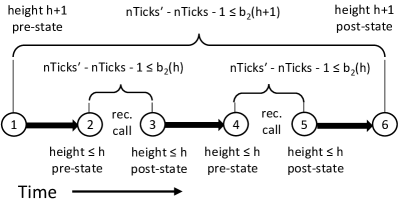
We then build up a height-$(h+1)$ summary, $\varphi_{h+1}$, compositionally, with $\varphi_{h}$ replacing the recursive calls. For example, consider the term $\tau_{2}=\texttt{nTicks}^{\prime}-\texttt{nTicks}-1$ in the context of Fig. 1. Our goal is to create a relational summary for the variable nTicks between labels 1 and 6. We do this by extending a summary for the transition between labels 1 and 2 with a summary for the transition between 2 and 3, namely, our hypothetical summary. Then we extend that with a summary for the paths between labels 3 and 4, and so on. Between labels 1 and 2, nTicks gets increased by 1. We then summarize the transition between 1 and 3. We know nTicks gets increased by 1 between labels 1 and 2. Furthermore, our hypothetical bounding function $\texttt{nTicks}^{\prime}-\texttt{nTicks}-1\leq b_{2}(h)$ says that nTicks gets increased by at most $b_{2}(h)+1$ between labels 2 and 3. Combining these summaries, we see that nTicks gets increased by at most $b_{2}(h)+2$ between labels 1 and 3. nTicks does not change between labels 3 and 4, so the summary between labels 1 and 4 is the same as the one between labels 1 and 3. The transition between labels 4 and 5 is a recursive call, so we again use our hypothetical summary to approximate this transition. Once again, such a summary says nTicks gets increased by at most $b_{2}(h)+1$. Extending our summary for the transition between 1 and 4 with this information allows us to conclude that nTicks gets increased by at most $2b_{2}(h)+3$ between labels 1 and 5. nTicks does not change between labels 5 and 6. Consequently, our summary for nTicks between labels 1 and 6 is $\texttt{nTicks}^{\prime}-\texttt{nTicks}\leq 2b_{2}(h)+3$. Similar reasoning would also obtain a summary for return as $\texttt{return}^{\prime}\leq 1+b_{1}(h)$. These formulas constitute our height-$(h+1)$ hypothetical summary, $\varphi_{h+1}$.

$$\varphi_{h+1}~{}\buildrel\mbox{\tiny\rm def}\over{=}~{}\texttt{return}^{\prime}\leq 1+b_{1}(h)~{}\land~{}\texttt{nTicks}^{\prime}\leq\texttt{nTicks}+2b_{2}(h)+3$$

If we rearrange each conjunct to respectively place $\tau_{1}$ and $\tau_{2}$ on the left-hand-side of each inequality, we obtain height-$(h+1)$ bounds on the values of $\tau_{1}$ and $\tau_{2}$. By definition such bounds are valid expressions for $b_{1}(h+1)$ and $b_{2}(h+1)$. That is at height-$(h+1)$,

(1) $$\texttt{return}^{\prime} \leq b_{1}(h)+1=b_{1}(h+1)$$

(2) $$\texttt{nTicks}^{\prime}-\texttt{nTicks}-1 \leq 2+2b_{2}(h)=b_{2}(h+1)$$

The equations give recursive definitions for $b_{1}$ and $b_{2}$. Solving these recurrence relations give us bounds on the value sets $V_{1}(h)$ and $V_{2}(h)$, for all heights $h$.

In §4.2, we present an algorithm that determines an upper bound on a procedure’s depth of recursion as a function of the parameters to the initial call and the values of global variables. This depth of recursion can also be interpreted as a stack height $h$ that we can use as an argument to the bounding functions $b_{k}(h)$. In the case of subsetSumAux, we obtain the bound $h\leq\max(1,1+\texttt{n}-\texttt{i})$. The solutions to the recurrences discussed above, when combined with the depth bound, yield the following summary.

$$\texttt{nTicks}^{\prime} \leq\texttt{nTicks}+2^{h}-1~{}\land~{}\texttt{return}^{\prime}\leq h-1~{}\land~{}$$

$$h \leq\max(1,1+\texttt{n}-\texttt{i})$$

When subsetSum is called with some array size $n$, the maximum possible depth of recursion that can be reached by subsetSumAux is equal to $n$. In this way, we have established that the running time of subsetSum is exponential in $n$, and the return value is at most $n$.

3. Background

Relational semantics.

In the following, we give an abstract presentation of the relational semantics of programs. Fix a set Var of program variables. A state $\sigma:{\it State}{}\buildrel\mbox{\tiny\rm def}\over{=}{\it Var}{}\rightarrow\mathbb{Z}$ consist of an integer valuation for each program variable. A recursive procedure $P$ can be understood as a chain-continuous (and hence monotonic) function on state relations $\mathcal{F}\llbracket P\rrbracket:2^{{\it State}{}\times{\it State}{}}\rightarrow 2^{{\it State}{}\times{\it State}{}}$. The relational semantics $\mathcal{R}\llbracket P\rrbracket$ of $P$ is given as the limit of the ascending Kleene chain of $\mathcal{F}\llbracket P\rrbracket$:

$$R(P,0) =\emptyset$$

$$R(P,h+1) =\mathcal{F}\llbracket P\rrbracket(R(P,h))$$

$$\mathcal{R}\llbracket P\rrbracket =\bigcup_{h\in\mathbb{N}}R(P,h)$$

Operationally, for any $h$ we may view $R(P,h)$ as the input/output relation of $P$ on a machine with a stack limit of $h$ activation records. We can extend relational semantics to mutually recursive procedures in the natural way, by considering $\mathcal{F}\llbracket P\rrbracket$ to be function that takes as input a $k$-tuple of state relations (where $k$ is the number of mutually recursive procedures).

A transition formula $\varphi$ is a formula over the program variables ${\it Var}{}$ and an additional set ${\it Var}{}^{\prime}$ of “primed” copies, representing the values of the program variables before and after a computation. A transition relation $\varphi$ can be interpreted as a property that holds of a pair of states $(\sigma,\sigma^{\prime})$: we say that $(\sigma,\sigma^{\prime})$ satisfies $\varphi$ if $\varphi$ is true when each variable in ${\it Var}{}$ is interpreted according to $\sigma$, and each variable in ${\it Var}{}^{\prime}$ is interpreted according to $\sigma^{\prime}$. We use $\mathcal{R}\llbracket\varphi\rrbracket$ to denote the state relation consisting of all pairs $(\sigma,\sigma^{\prime})$ that satisfy $\varphi$. This paper is concerned with the problem of procedure summarization, in which the goal is to find a transition formula $\varphi$ that over-approximates a procedure, in the sense that $\mathcal{R}\llbracket P\rrbracket\subseteq\mathcal{R}\llbracket\varphi\rrbracket$.

A relational expression $\tau$ is a polynomial over ${\it Var}{}\cup{\it Var}{}^{\prime}$ with rational coefficients. A relational expression can be evaluated at a state pair $(\sigma,\sigma^{\prime})\in{\it State}\times{\it State}$ by using $\sigma$ to interpret the unprimed symbols and $\sigma^{\prime}$ to interpret the primed symbols—we use $\mathcal{E}\llbracket\tau\rrbracket(\sigma,\sigma^{\prime})$ to denote the evaluation of $\tau$ at $(\sigma,\sigma^{\prime})$.

Intra-procedural analysis.

The technique for procedure summarization developed in this paper makes use of intra-procedural summarization as a sub-routine. We formalize this intra-procedural technique by a function $\textit{PathSummary}(e,x,V,E)$, which takes as input a control-flow graph with vertices $V$, edges $E$, entry vertex $e$, and exit vertex $x$, and computes a transition formula that over-approximates all paths in $(V,E)$ between $e$ and $x$. We use $\textit{Summary}(P,\varphi)$ to denote a function that takes as input a recursive procedure $P$ and a transition formula $\varphi$, and computes a transition formula that over-approximates $P$ when $\varphi$ is used to interpret recursive calls (i.e., $\mathcal{F}\llbracket P\rrbracket(\mathcal{R}\llbracket\varphi\rrbracket)\subseteq\mathcal{R}\llbracket\textit{Summary}(P,\varphi)\rrbracket$). $\textit{Summary}(P,\varphi)$ can be implemented in terms of $\textit{PathSummary}(e,x,V,E)$ by replacing all call edges with $\varphi$, and taking $(e,x,V,E)$ to be the control-flow graph of $P$.

In principle, any intra-procedural summarization procedure can be used to implement $\textit{Summary}(P,\varphi)$; the implementation of our method uses the technique from Kincaid et al. (2018).

Input : Formula of the form $\exists X.\psi$ where $\psi$ is satisfiable and quantifier-free

Output : Convex hull of $\exists X.\psi$

1 $P\leftarrow\bot$;

2 while there exists a model $m$ of $\psi$ do

3    Let $Q$ be a cube of the DNF of $\psi$ s.t. $m\models Q$;

    $Q\leftarrow\textit{project}(Q,X)$ ;

     /* Polyhedral projection */

    $P\leftarrow P\sqcup Q$ ;

     /* Polyhedral join */

4    $\psi\leftarrow\psi\land\lnot P$;

5   

return $P$

Algorithm 1 The convex-hull algorithm from (Farzan and Kincaid, 2015)

Symbolic abstraction.

We use $\textit{Abstract}(\varphi,V)$ to denote a procedure that takes a formula $\varphi$ and computes a set of polynomial inequations over the variables $V$ that are implied by $\varphi$. If $\varphi$ is expressed in linear arithmetic, then a representation of all implied polynomial inequations (namely, a constraint representation of the convex hull of $\varphi$ projected onto $V$) can be computed effectively (e.g., using (Farzan and Kincaid, 2015, Alg. 2), which we show in this paper as Alg. 1). Otherwise, we settle for a sound procedure that produces inequations implied by $\varphi$, but not necessarily all of them (e.g., using (Kincaid et al., 2018, Alg. 3)).

In principle, the convex hull of a linear arithmetic formula F can be computed as follows: write F in disjunctive normal form, as $F\equiv C_{1}\lor...\lor C_{n}$, where each $C_{i}$ is a conjunction of linear inequations (i.e., a convex polyhedron). The convex hull of $F$ is obtained by replacing disjunctions with the join operator of the domain of convex polyhedra. This algorithm can be improved by using an SMT solver to enumerate the DNF lazily, and extended to handle existential quantification by using polyhedral projection (Alg. 1). A similar approach can be used to compute a conjunction of non-linear inequations that are implied by a formula $F$, by treating non-linear terms in the formula as additional dimensions of the space (e.g., a quadratic inequation $x^{2}<y^{2}$ is treated as a linear inequation $d_{x^{2}}<d_{y^{2}}$, where $d_{x^{2}}$ and $d_{y^{2}}$ are symbols that we associate with the terms $x^{2}$ and $y^{2}$, but have no intrinsic meaning). The non-linear variation of the algorithm’s precision can be improved by using inference rules, congruence closure, and Grobner-basis algorithms to deduce linear relations among the non-linear dimensions that are consequences of the non-linear theory ((Kincaid et al., 2018, Alg. 3)). Note that, because non-linear integer arithmetic is undecidable, this process is (necessarily) incomplete.

Recurrence relations.

C-finite sequences are a well-studied class of sequences defined by linear recurrence relations, of which a famous example is the Fibonacci sequence. Formally,

Definition 3.1.

A sequence $s:\mathbb{N}\rightarrow\mathbb{Q}$ is $C$-finite of order $d$ if it satisfies a linear recurrence equation

$$s(k+d)=c_{1}s(k+d-1)+...+c_{d-1}s(k+1)+c_{d}s(k)\ ,$$

where each $c_{i}$ is a constant.

It is classically known that every C-finite sequence $s(k)$ admits a closed form that is computable from its recurrence relation and takes the form of an exponential-polynomial

$$s(k)=p_{1}(k)r_{1}^{k}+p_{2}(k)r_{2}^{k}+...+p_{l}(k)r_{l}^{k}\ ,$$

where each $p_{i}$ is a polynomial in $k$ and each $r_{i}$ is a constant. In the following, it will be convenient to use a different kind of recurrence relation to present $C$-finite sequences, namely stratified systems of polynomial recurrences.

Definition 3.2.

A stratified system of polynomial recurrences is a system of recurrence equations over sequences $x_{1,1},...,x_{1,n_{1}},...,x_{m,1},...,x_{m,n_{m}}$ of the form

$$\{x_{i,j}(k+1)=c_{i,j,1}x_{i,1}(k)+\dotsi+c_{i,j,n_{i}}x_{i,n_{i}}(k)+p_{i,j}\}_{i,j}$$

where each $c_{i,j,1},...,c_{i,j,n_{i}}$ is a constant, and $p_{i,j}$ is a polynomial in $x_{1,1}(k),...,x_{1,n_{1}}(k),...,x_{i-1,1}(k),...,x_{i-1,n_{i-1}}(k)$.

Intuitively, the sequences $x_{1,1},...,x_{1,n_{1}},...,x_{m,1},...,x_{m,n_{m}}$ are organized into strata ($x_{1,1},...,x_{1,n_{1}}$ is the first, $x_{2,1},...,x_{2,n_{1}}$ is the second, and so on), the right-hand-side of the equation for $x_{i,j}$ can involve linear terms over the sequences in the $i^{\textit{th}}$ strata, and additional polynomial terms over sequences of lower strata. It follows from the closure properties of C-finite sequences that each $x_{i,j}$ defines a $C$-finite sequence, and an exponential-polynomial closed form for each sequence can be computed from a stratified system of polynomial recurrences (Kauers and Paule, 2011). The fact that any $C$-finite sequence satisfies a stratified system of polynomial recurrences follows from the fact that a recurrence of order $d$ can be implemented as a system of linear recurrences among $d$ sequences (Kauers and Paule, 2011).

Example 3.3.

An example of a stratified system of polynomial recurrences with four sequences ($w,x,y,z$) arranged into two strata ($(w,x)$ and $(y,z)$) is as follows:

$$\begin{bmatrix}w(k+1)\\ x(k+1)\end{bmatrix} =\begin{bmatrix}1&\frac{1}{3}\\ 0&2\end{bmatrix}\begin{bmatrix}w(k)\\ x(k)\end{bmatrix}+\begin{bmatrix}1\\ 0\end{bmatrix}$$

$$\begin{bmatrix}y(k+1)\\ z(k+1)\end{bmatrix} =\begin{bmatrix}1&0\\ 1&1\end{bmatrix}\begin{bmatrix}y(k)\\ z(k)\end{bmatrix}+\begin{bmatrix}x(k)^{2}+1\\ 3w(k)+x(k)\end{bmatrix}$$

This system has the closed-form solution

$$w(k) =w(0)+\frac{(2^{k}-1)}{3}x(0)+k\qquad x(k)=2^{k}x(0)$$

$$y(k) =\frac{4^{k}-1}{3}x(0)^{2}+y(0)+k$$

$$z(k) =3w(0)+\frac{4^{k}-3k-1}{9}x(0)^{2}+$$

$$\qquad(2^{k+1}-k-1)x(0)+ky(0)+z(0)+2(k^{2}-k)\ .$$

4. Technical Details

This section gives algorithms for summarizing recursive procedures using recurrence solving. We assume that before these algorithms are applied to the procedures of a program $\mathcal{P}$, we first compute and collapse the strongly connected components of the call graph of $\mathcal{P}$ and topologically sort the collapsed graph. Our analysis then works on the strongly connected components of the call graph in a single pass, in a topological order of the collapsed graph, by applying the algorithms of this section to recursive components, and applying intraprocedural analysis to non-recursive components.

For simplicity, §4.1 focuses on the analysis of strongly connected components consisting of a single recursive procedure $P$. The first step of the analysis is to apply Alg. 2, which produces a set of inequations that describe the values of variables in $P$. Not all of the inequations found by Alg. 2 are suitable for use in a recurrence-based analysis, so we apply Alg. 3 to filter the set of inequations down to a subset that, when combined, form a stratified recurrence. The next step is to give this recurrence to a recurrence solver, which results in a logical formula relating the values of variables in $P$ to the stack height $h$ that may be used by $P$. In §4.2, we show how to (i) obtain a bound on $h$ that depends on the program state before the initial call to $P$, and (ii) combine the recurrence solution with that depth bound to create a summary of $P$. In §4.3, we discuss how to obtain a certain class of more precise bounds (including lower bounds on the running time of a procedure). In §4.4, we show how to extend the techniques of §4.1 to handle programs with mutual recursion, i.e., programs whose call graphs have strongly connected components consisting of multiple procedures. In §4.5, we discuss an extension of the algorithm of §4.4 that handles sets of mutually recursive procedures in which some procedures do not have base cases.

4.1. Height-Based Recurrence Analysis

Let $\tau$ be a relational expression and let $P$ be a procedure. We use $V_{\tau}(P,h)$ to denote the set of values of $\tau$ in a height-$h$ execution of $P$.

$$V_{\tau}(P,h)\buildrel\mbox{\tiny\rm def}\over{=}\{\mathcal{E}\llbracket\tau\rrbracket(\sigma,\sigma^{\prime}):(\sigma,\sigma^{\prime})\in R(P,h)\}$$

It consists of values to which $\tau$ may evaluate at a state pair belonging to $R(P,h)$. We call $b_{\tau}:\mathbb{N}\rightarrow\mathbb{Q}$ a bounding function for $\tau$ in $P$ if for all $h\in\mathbb{N}$ and all $v\in V_{\tau}(P,h)$, we have $v\leq b_{\tau}(h)$. Intuitively, the bounding function $b_{\tau}(h)$ bounds the value of an expression $\tau$ in any execution that uses stack height at most $h$.

The goal of §4.1 is to find a set of relational expressions and associated bounding functions. We proceed in three steps. First, we determine a set of candidate relational expressions $\tau_{1},...,\tau_{n}$. Second, we optimistically assume that there exist functions $b_{1}(h),...,b_{n}(h)$ that bound these expressions, and we analyze $P$ under that assumption to obtain constraints relating the values of the relational expressions to the values of the $b_{1}(h),...,b_{n}(h)$ functions. Third, we re-arrange the constraints into recurrence relations for each of the $b_{k}(h)$ functions (if possible) and solve them to synthesize a closed-form expression for $b_{k}(h)$ that is suitable to be used in a summary for $P$.

We begin our analysis of $P$ by determining a set of suitable expressions $\tau$. If a relational expression $\tau$ has an associated bounding function, then it must be the case that $V_{\tau}(P,1)$ (i.e., the set of values that $\tau$ takes on in the base case) is bounded above. Without loss of generality, we choose expressions $\tau$ so that $V_{\tau}(P,1)$ is bounded above by zero. (Note that if $V_{\tau}(P,1)$ is bounded above by $c$ then $V_{\tau-c}(P,1)$ is bounded above by zero.) We begin our analysis of $P$ by analyzing the base case to look for relational expressions that have this property.

Input : A procedure $P$, and the associated vocabulary of program variables Var

Output : Height-based-recurrence summary $\varphi_{\textit{height}}$

1 $\beta\leftarrow\textit{Summary}(P,\textit{false})$ ;

2 $w_{\textit{base}}\leftarrow\textit{Abstract}(\beta,\textit{Var}\cup\textit{Var}^{\prime})$ ;

3 $n\leftarrow$ the number of inequations in $w_{\textit{base}}$;

4 foreach $k$ in $1,...,n$ do

5    Let $\tau_{k}$ be the expression over $\textit{Var}\cup\textit{Var}^{\prime}$ such that the $k^{\textrm{th}}$ inequation in $w_{\textit{base}}$ is $(\tau_{k}\leq 0)$ ;

6    Let $b_{k}(\cdot)$ be a fresh uninterpreted function symbol ;

7   

8    $\varphi_{\textit{call}}\leftarrow\bigwedge_{k=1}^{n}(\tau_{k}\leq b_{k}(h)\land b_{k}(h)\geq 0)$ ;

9    $\varphi_{\textit{rec}}\leftarrow\textit{Summary}(P,\varphi_{\textit{call}})$ ;

10    $\varphi_{\textit{ext}}\leftarrow\varphi_{\textit{rec}}\land\bigwedge_{k=1}^{n}(b_{k}(h+1)=\tau_{k})$ ;

11    $S\leftarrow\emptyset$;

12    foreach $k$ in $1,...,n$ do

13       $w_{\textit{ext},k}\leftarrow\textit{Abstract}(\varphi_{\textit{ext}},\{b_{1}(h),...,b_{n}(h),b_{k}(h+1)\})$ ;

14       foreach inequation $\mathcal{I}$ in $w_{\textit{ext},k}$ do

15          $S\leftarrow S\cup\{\mathcal{I}\}$

16         

return $S$

Algorithm 2 Algorithm for extracting candidate recurrence inequations

Selecting candidate relational expressions.

The reason for looking at expressions over program variables, as opposed to individual variables, is illustrated by Ex. 2.1: the variable nTicks has a different value each time the base case executes, but the expression $\texttt{nTicks}^{\prime}-\texttt{nTicks}-1$ is always equal to zero in the base case.

With the goal of identifying relational expressions that are bounded above by zero, Alg. 2 begins by extracting a transition formula $\beta$ for the non-recursive paths through $P$ by calling $\textit{Summary}(P,\textit{false})$ (i.e., summarizing $P$ by using false as a summary for the recursive calls in $P$). Next, we compute a set $w_{\textit{base}}$ of polynomial inequations over $\textit{Var}\cup\textit{Var}^{\prime}$ (the set of un-primed (pre-state) and primed (post-state) copies of all global variables, along with unprimed copies of the parameters to $P$ and the variable $\texttt{return}^{\prime}$, which represents the return value of $P$) that are implied by $\beta$ by calling $\textit{Abstract}(\beta,\textit{Var}\cup\textit{Var}^{\prime})$. Let $n$ be the number of inequations in $w_{\textit{base}}$. Then, for $k=1,...,n$, we rewrite the $k^{th}$ inequation in the form $\tau_{k}\leq 0$. In the case of Ex. 2.1, $\tau_{1}\buildrel\mbox{\tiny\rm def}\over{=}\texttt{return}^{\prime}$ and $\tau_{2}\buildrel\mbox{\tiny\rm def}\over{=}\texttt{nTicks}^{\prime}-\texttt{nTicks}-1$ have the property that $\tau_{1}\leq 0$ and $\tau_{2}\leq 0$ in the base case.

Note that there are, in general, many sets of relational expressions $\tau_{1},...,\tau_{n}$ that are bounded above by zero in the base case. The soundness of Alg. 2 only depends on Abstract choosing some such set. Our implementation of Abstract uses (Kincaid et al., 2018, Alg. 3), and is not guaranteed to choose the set of relational expressions that would lead to the most precise results for any given application, e.g., for a given assertion-checking or complexity-analysis problem. Intuitively, in the case that $\beta$ is a formula in linear arithmetic, our implementation of Abstract amounts to using the operations of the polyhedral abstract domain to find a convex hull of $\beta$. Then, each of the inequations in the constraint representation of the convex hull can be interpreted as a relational expression that is bounded above by zero in the base case.

Generating constraints on bounding functions.

For each of the expressions $\tau_{k}$ that has an upper bound in the base case, we are ultimately looking to find a function $b_{k}(h)$ that is an upper bound on the value of that expression in any height-$h$ execution. Our way of finding such a function is to analyze the recursive cases of $P$ to look for an invariant inequation that gives an upper bound on $V_{\tau_{k}}(P,h+1)$ in terms of an upper bound on $V_{\tau_{k}}(P,h)$. Such an inequation can be interpreted as a recurrence relating $b_{k}(h+1)$ to $b_{k}(h)$.

The remainder of Alg. 2 (Lines (2)–(2)) finds such invariant inequations. The first step is to create the hypothetical procedure summary $\varphi_{\textit{call}}$, which hypothesizes that a bounding function $b_{\tau_{k}}$ exists for each expression $\tau_{k}$, and that the value of that function at height $h$ is an upper bound on the value of $\tau_{k}$. $\varphi_{\textit{call}}$ is a transition formula that represents a height-$h$ execution of $P$. In Ex. 2.1, $\varphi_{\textit{call}}$ is:

$$\texttt{return}^{\prime} \leq b_{1}(h)\land\texttt{nTicks}^{\prime}-\texttt{nTicks}-1\leq b_{2}(h)\land$$

$$b_{1}(h) \geq 0\land b_{2}(h)\geq 0$$

On line (2), Alg. 2 calls Summary, using $\varphi_{\textit{call}}$ as the representation of each recursive call in $P$, and the resulting transition formula is stored in $\varphi_{\textit{rec}}$. Thus, $\varphi_{\textit{rec}}$ describes a typical height-$(h+1)$ execution of $P$. In Ex. 2.1, a simplified version of $\varphi_{\textit{rec}}$ is given as $\varphi_{h+1}$ in §2.

On line (2), the formula $\varphi_{\textit{ext}}$ is produced by conjoining $\varphi_{\textit{rec}}$ with a formula stating that, for each $k$, $b_{k}(h+1)=\tau_{k}$. Therefore, $\varphi_{\textit{ext}}$ implies that any upper bound on $b_{k}(h+1)$ must be an upper bound on $\tau_{k}$ in any height-$(h+1)$ execution.

Ultimately, we wish to obtain a closed-form solution for each $b_{k}(h)$. The formula $\varphi_{\textit{ext}}$ implicitly determines a set of recurrences relating $b_{1}(h+1),...,b_{n}(h+1)$ to $b_{1}(h),...,b_{n}(h)$. However, $\varphi_{\textit{ext}}$ does not have the explicit form of a recurrence. Lines (2)–(2) abstract $\varphi_{\textit{ext}}$ to a conjunction of inequations that give an explicit relationship between $b_{k}(h+1)$ and $b_{1}(h),...,b_{n}(h)$ for each $k$.

Input : A set of candidate inequations $\mathcal{I}_{1},...,\mathcal{I}_{N}$ over the function symbols $b_{1}(h),...,b_{n}(h),b_{1}(h+1),...,b_{n}(h+1)$

Output : A set of inequations that form a stratified recurrence

1 Let $\textit{DefinesBound}[j]$ be a map from integers to integers;

2 Let $\textit{UsesBound}[j,k]$ and $\textit{UsesBoundNonLinearly}[j,k]$ be maps that map all pairs of integers to false;

3 $S\leftarrow\{1,...,N\}$ ;

4 foreach $j$ in $1,...,N$ do

5    Write $\mathcal{I}_{j}$ as $b_{k}(h+1)\leq c_{0}+\Sigma_{i=1}^{m_{j}}c_{i}(b_{1}(h))^{d_{i,1}}\cdots(b_{n}(h))^{d_{i,n}}$ if $\mathcal{I}_{j}$ can be written in that form with $1\leq k\leq n$, $\forall i.~{}c_{i}\in\mathbb{Q}$, $\exists i>0.~{}c_{i}>0$, $\forall i,p.~{}d_{i,p}\in\mathbb{N}$; otherwise let $S\leftarrow S-\{j\}$ and continue loop;

6    For $i=0,...,m_{j}$, $c_{i}^{\prime}\leftarrow\max(0,c_{i})$ ;

7    Let $\mathcal{I}_{j}^{\prime}$ be $b_{k}(h+1)\leq c_{0}^{\prime}+\Sigma_{i=1}^{m_{j}}c_{i}^{\prime}(b_{1}(h))^{d_{i,1}}\cdots(b_{n}(h))^{d_{i,n}}$;

8    $\textit{DefinesBound}[j]:=k$;

9    foreach $i\in\{1,..,m_{j}\}$ do

10       foreach $p\in\{1,...,n\}$ do

11          if $c_{i}^{\prime}>0\land d_{i,p}>0$ then  $\textit{UsesBound}[j,p]:=\textit{true}$ ;

12          if $c_{i}^{\prime}>0\land d_{i,p}>0\land\Sigma_{q=1}^{n}d_{i,q}>1$ then  $\textit{UsesBoundNonLinearly}[j,p]:=\textit{true}$ ;

13         

14         

15         

16          $A\leftarrow\emptyset$ ;

17          repeat

18             $V\leftarrow S-A$;

19             repeat

20                foreach $j\in V$ do

21                   if $\exists k.\textit{UsesBound}[j,k]\land\lnot\exists j^{\prime}\in V.\textit{DefinesBound}[j^{\prime}]=k$  then $V\leftarrow V-\{j\}$;

22                   if $\exists k.\textit{UsesBoundNonLinearly}[j,k]\land\lnot\exists j^{\prime}\in A.\textit{DefinesBound}[j^{\prime}]=k$  then $V\leftarrow V-\{j\}$;

23                  

24                  

25                   until $V$ is unchanged;

26                  foreach $k=\{1,...,n\}$ do

27                      if $V$ contains more than one $j$ such that $\textit{DefinesBound}[j]=k$ then

28                         Arbitrarily choose one such $j$ to remain in $V$, and remove all other such $j$ from $V$ ;

29                        

30                         $A\leftarrow A\cup V$;

31                        

32                         until $V=\emptyset$;

return $\{\mathcal{I}_{j}^{\prime}\mid j\in A\}$

Algorithm 3 Algorithm for constructing a stratified recurrence

Extracting and solving recurrences.

The next step of height-based recurrence analysis is to identify a subset of the inequations returned by Alg. 2 that constitute a stratified system of polynomial recurrences (Defn. 3.2). This subset must meet the following three stratification criteria:

1. Each bounding function $b_{k}(h+1)$ must appear on the left-hand-side of at most one inequation.

2. If a bounding function $b_{k}(h)$ appears on the right-hand-side of an inequation, then $b_{k}(h+1)$ appears on some left-hand-side.

3. It must be possible to organize the $b_{k}(h+1)$ into strata, so that if $b_{k}(h)$ appears in a non-linear term on the right-hand-side of the inequation for $b_{j}(h+1)$, then $b_{k}(h)$ must be on a strictly lower stratum than $b_{k}(h)$.

Alg. 3 computes a maximal subset of inequations that complies with the above three rules.

The next step of height-based recurrence analysis is to send this recurrence to a recurrence solver, such as the one described in Kincaid et al. (2018). The solution to the recurrence is a set of bounding functions. Let $B$ be the set of indices $k$ such that we found a recurrence for, and obtained a closed-form solution to, the bounding function $b_{k}(h)$. Using these bounding functions, we can derive the following procedure summary for $P$, which leaves the height $H$ unconstrained.

(3) $$\exists H.\bigwedge_{k\in B}[\tau_{k}\leq b_{k}(H)]$$

The subject of §4.2 is to find a formula $\zeta_{P_{i}}(H,\sigma)$ relating $H$ to the pre-state $\sigma$ of the initial call to $P$. The formula $\zeta_{P_{i}}(H,\sigma)$ can be combined with Eqn. (3) to obtain a more precise procedure summary.

Soundness.

Roughly, the soundness of height-based recurrence analysis follows from: (i) sound extraction of the recurrence constraints used by CHORA to characterize non-linear recursion; (ii) sound recurrence solving; and (iii) soundness of the underlying framework of algebraic program analysis. The soundness of parts (ii) and (iii) depends on the soundness of prior work (Kincaid et al., 2018). The soundness of (i) is addressed in a detailed proof in the appendix of this document. The soundness property proved there is as follows: let $P$ be a procedure to which Alg. 2 and Alg. 3 have been applied to obtain a stratified recurrence. Let $\{\tau_{i}\}_{i\in[1,n]}$ be the relational expressions computed by Alg. 2. Let $B\subseteq[1,n]$ be such that $\{b_{i}\}_{i\in B}$ is the set of functions produced by solving the stratified recurrence. We show that each $b_{i}$ function bounds the corresponding $V_{\tau_{i}}(P,h)$ value set. In other words, the following statement holds: $\forall h\geq 1.\bigwedge_{i\in B}\forall v\in V_{\tau_{i}}(P,h).v\leq b_{i}(h)$.

4.2. Depth-Bound Analysis

Input : A weighted control-flow graph $(V,E,C)$

Output : Depth-bound formulas $\zeta_{P_{1}}(D,\sigma),...,\zeta_{P_{n}}(D,\sigma)$

1 foreach $i\in\{1,...n\}$ do

2   Let $e_{P_{i}}^{\prime}$ be a new vertex

3    Let $x^{\prime}$ be a new vertex;

4    $V^{\prime}\leftarrow V\cup\{x^{\prime}\}\cup\{e_{P_{i}}^{\prime}\mid i\in\{1,...,n\}\}$;

5    Create a new integer-valued auxiliary variable $D$;

6    $E^{\prime}\leftarrow E$;

7    foreach $i\in\{1,...,n\}$ do

8       $E^{\prime}\leftarrow E^{\prime}\cup\{(e_{P_{i}}^{\prime},\varphi_{[D:=1]},e_{P_{i}})$} $\cup\{(e_{P_{i}},\beta_{P_{i}},x^{\prime})$}

9       foreach call edge $(u,Q,v)$ in $C$ do

10          if $Q=P_{i}$ for some $i$ then

11             $E^{\prime}\leftarrow E^{\prime}\cup\{(u,\varphi_{[D:=D+1]},e_{Q})\}\cup\{(u,\varphi_{[havoc]},v)\}$

12             else

13                $E^{\prime}\leftarrow E^{\prime}\cup\{(u,\varphi_{Q},v)\}$

14               

15                foreach $i=1,...,n$ do

16                   $\zeta_{P_{i}}(D,\sigma)\leftarrow\textrm{PathSummary}\,(e_{P_{1}}^{\prime},x^{\prime},V^{\prime},E^{\prime},\emptyset)$

return $\zeta_{P_{1}}(D,\sigma),...,\zeta_{P_{n}}(D,\sigma)$

Algorithm 4 Algorithm for producing a depth-bound formula

In §4.1, we showed how to find a bounding function $b_{\tau}(h)$ that gives an upper bound on the value of a relational expression $\tau$ in an execution of a procedure $P_{i}$ as a function of the stack height (i.e., maximum depth of recursion) $h$ of that execution. In this section, the goal is to find bounds on the maximum depth of recursion $h$ that may occur as a function of the pre-state $\sigma$ (which includes the values of global variables and parameters to $P_{i}$) from which $P_{i}$ is called.

For example, consider Ex. 2.1. The algorithms of §4.1 determine bounds on the values of two relational expressions in terms of $h$, namely: $\texttt{nTicks}^{\prime}\leq\texttt{nTicks}+2^{h}-1$, and $\texttt{return}^{\prime}\leq h-1$. The algorithm of this sub-section (Alg. 4) determines that $h$ satisfies $h\leq\max(1,1+\texttt{n}-\texttt{i})$. These facts can be combined to form a procedure summary for SubsetSumAux that relates the return value and the increase to nTicks to the values of the parameters i and n.

The stack height $h$ required to execute a procedure often depends on the number of times that some transformation can be applied to the procedure’s parameters before a base case must execute. For example, in Ex. 2.1, the height bound is a consequence of the fact that i is incremented by one at each recursive call, until $\texttt{i}\geq\texttt{n}$, at which point a base case executes. Likewise, in a typical divide-and-conquer algorithm, a size parameter is repeatedly divided by some constant until the size parameter is below some threshold, at which point a base case executes. Intuitively, the technique described in this section is designed to discover height bounds that are consequences of such repeated transformations (e.g., addition or division) applied to the procedures’ parameters.

To achieve this goal, we use Alg. 4, which is inspired by the algorithm for computing bounds on the depth of recursion in Albert et al. (2013). Alg. 4 constructs and analyzes an over-approximate depth-bounding model of the procedures $P_{1},...,P_{n}$ that includes an auxiliary depth-counter variable, $D$. Each time that the model descends to a greater depth of recursion, $D$ is incremented. The model exits only when a procedure executes its base case. In any execution of the model, the final value of $D$ thus represents the depth of recursion at which some procedure’s base case is executed.

Alg. 4 takes as input a representation of the procedures in $S$ as a single, combined control-flow graph $(V,E,C)$ having two kinds of edges: (1) weighted edges $(u,\varphi,v)\in E$, which are weighted with a transition formula $\varphi$, and (2) call edges in the set $C$. Each call edge in $C$ is a triple $(u,Q,v)$, in which $u$ is the call-site vertex, $v$ is the return-site vertex, and the edge is labeled with $Q$, representing a call to a procedure $Q$. We assume that if any procedure $Q\notin S$ is called by some procedure in $S$, then $Q$ has been fully analyzed already, and therefore a procedure summary $\varphi_{Q}$ for $Q$ has already been computed. Each procedure $Q$ has an entry vertex $e_{Q}$, an exit vertex $x_{Q}$, and a transition formula $\beta_{Q}$ that over-approximates the base cases of $Q$. Note that $(V,E,C)$ consists of several disjoint, single-procedure control-flow graphs when $n>1$.

On lines (4)–(4), Alg. 4 constructs the depth-bounding model, represented as a new control-flow graph $(V^{\prime},E^{\prime},\emptyset)$. The algorithm begins by creating new auxiliary entry vertices $e_{P_{1}}^{\prime},...,e_{P_{n}}^{\prime}$ for the procedures $P_{1},...,P_{n}$ and a new auxiliary exit vertex $x^{\prime}$. The new vertex set $V^{\prime}$ contains $V$ along with these $n+1$ new vertices. Alg. 4 then creates a new integer-valued variable $D$. For $i=1,...,n$, the algorithm then creates an edge from $e_{P_{i}}^{\prime}$ to $e_{P_{i}}$, weighted with a transition formula that initializes $D$ to one, and an edge from $x_{P_{i}}$ weighted with the formula $\beta_{P_{i}}$, which is a summary of the base case of $P_{i}$.

Alg. 4 replaces every call edge $(u,Q,v)\in C$ with one or more weighted edges. Each call to a procedure $Q\notin\{P_{1},...,P_{n}\}$ is replaced by an edge $(u,\varphi_{Q},v)$ weighted with the procedure summary $\varphi_{Q}$ for $Q$. Each call to some $P_{i}$ is replaced by two edges. The first edge represents descending into $P_{i}$, and goes from $u$ to $e_{P_{i}}$, and is weighted with a formula that increments $D$ and havocs local variables. The second edge represents skipping over the call to $P_{i}$ rather than descending into $P_{i}$. This edge is weighted with a transition formula that havocs all global variables and the variable return, but leaves local variables unchanged.

The final step of Alg. 4, on line (4), actually computes the depth-bounding summary $\zeta_{P_{i}}(D,\sigma)$ for each procedure $P_{i}$. Because there are no call edges in the new control-flow graph $(V^{\prime},E^{\prime},\emptyset)$, intraprocedural-analysis techniques can be used to compute transition formulas that summarize the transition relation for all paths between two specified vertices. For each procedure $P_{i}$, the formula $\zeta_{P_{i}}(D,\sigma)$ is a summary of all paths from $e_{P_{i}}^{\prime}$ to $x^{\prime}$, which serves to relate $D$ to $\sigma$, which is the pre-state of the initial call to $P_{i}$.

The formulas $\zeta_{P_{i}}(D,\sigma)$ for $i=1,...,n$ can be used to establish an upper bound on the depth of recursion in the following way. Let $(\sigma,\sigma^{\prime})$ be a state pair in the relational semantics $\mathcal{R}\llbracket P_{i}\rrbracket$ of $P_{i}$. Then, there is an execution $e$ of $P_{i}$ that starts in state $\sigma$ and finishes in state $\sigma^{\prime}$, in which the maximum recursion depth is some $d\in\mathbb{N}$. Then there is a path through the control-flow graph $(V^{\prime},E^{\prime},\emptyset)$ that corresponds to the path taken in $e$ to reach some execution of a base case at the maximum recursion depth $d$. Therefore, if $d$ is a possible depth of recursion when starting from state $\sigma$, then there is a satisfying assignment of $\zeta_{P_{i}}(D,\sigma)$ in which $D$ takes the value $d$. The contrapositive of this argument says that, if there does not exist any satisfying assignment of $\zeta_{P_{i}}(D,\sigma)$ in which $D$ takes the value $d$, then it must be the case that no execution of $P_{i}$ that starts in state $\sigma$ can have maximum recursion depth $d$. In this way, $\zeta_{P_{i}}(D,\sigma)$ can be interpreted as providing bounds on the maximum recursion depth that can occur when $P_{i}$ is started in state $\sigma$.

Once we have the depth-bound summary $\zeta_{P}$ for some procedure $P$, we can combine it with the closed-form solutions for bounding functions that we obtained using the algorithms of §4.1 to produce a procedure summary. Let $B$ be the set of indices $k$ such that we found a recurrence for the bounding function $b_{k}(h)$. We produce a procedure summary of the form shown in Eqn. (4), which uses the depth-bound summary $\zeta_{P}$ to relate the pre-state $\sigma$ to the variable $H$, which in turn is used to index into the bounding function $b_{k}(h)$ for each $k\in B$.

(4) $$\exists H.\zeta_{P}(H,\sigma)\land\bigwedge_{k\in B}[\tau_{k}\leq b_{k}(H)]$$

4.3. Finding Lower Bounds Using Two-Region Analysis

In this sub-section, we describe an extension of height-based recurrence analysis, called two-region analysis, that is able to prove stronger conclusions, such as non-trivial lower bounds on the running times of some procedures.

In §4.1, we discussed height-based recurrence analysis, and showed how it can find an upper bound on the increase to the variable nTicks in Ex. 2.1. Now, we consider the application of height-based recurrence analysis to the procedure differ shown in Fig. 2. differ uses the global variables x and y to (in effect) return a pair of integers. The pair $(\texttt{x},\texttt{y})$ returned by the procedure is formed from the x value returned by the first call and the y value returned by the second call, each incremented by one. The base case occurs when the parameter n equals zero or one, and at each call site, the parameter n is decreased by either one or two. We will apply height-based recurrence analysis and two-region analysis to look for bounds on $\texttt{x}^{\prime}$ and $\texttt{y}^{\prime}$, and their sum and difference, after differ is called with a given value n.

For the purposes of the following discussion, we will focus on x, but the same conclusions apply to y. By applying height-based recurrence analysis to the procedure differ, we can prove that the post-state value $\texttt{x}^{\prime}$ is upper-bounded by $\texttt{n}-1$. At the same time, the analysis also proves a lower bound on $\texttt{x}^{\prime}$ by considering the term $\tau_{1}=-\texttt{x}^{\prime}$. However, the bounding function $b_{1}(h)$ obtained by height-based analysis is the constant function $b_{1}(h)=0$, which yields the trivial lower bound $\texttt{x}^{\prime}\geq 0$. As a result, the results of height-based recurrence analysis can only be used to prove that the difference between $\texttt{x}^{\prime}$ and $\texttt{y}^{\prime}$ is at most $\texttt{n}-1$, which is an over-estimate by a factor of two.

$\begin{array}[]{@{\hspace{0ex}}c@{\hspace{5.0ex}}c@{\hspace{0ex}}}{\begin{array}[]{l}\textrm{int}~{}x;~{}\textrm{int}~{}y;\\ \textrm{int}~{}\textit{differ}(\textrm{int}~{}n)~{}\{\\ \hskip 14.22636pt\textbf{if}~{}(n==0~{}||~{}n==1)~{}\{~{}x=0;~{}y=0;~{}\textbf{return};\}\\ \hskip 14.22636pt\textit{differ}(nondet()~{}?~{}n-1:n-2);\\ \hskip 14.22636pt\textrm{int}~{}temp~{}=~{}x;\textit{// Store x ``returned'' by first call}\\ \hskip 14.22636pt\textit{differ}(nondet()~{}?~{}n-1:n-2);\\ \hskip 14.22636ptx=temp+1;y=y+1;\textit{// ``Return'' (temp+1,y+1)}\\ \}\end{array}}\hfil\hskip 21.52771pt\\ {\parbox[c]{142.26378pt}{ \includegraphics[width=144.54pt]{figures/dual-height-diagram} }}\hfil\hskip 21.52771pt\end{array}$

Figure 2. Source code for the non-linearly recursive procedure differ, and a depiction of a possible tree of recursive calls differ. The number inside each vertex indicates the value of the parameter $n$ at that execution of differ. The minimum depth $M$ at which a base case occurs in this recursion tree is 3. The upper region of the tree, which includes all vertices at depth less than or equal to $M$, is shown with bold outlines.

In this sub-section, we extend our formal characterization of the relational semantics of a procedure (given in §3) in the following way. We use $V_{\tau}(R)$ to denote the set of values that $\tau$ takes on in a state relation $R$. That is, $V_{\tau}(R)\buildrel\mbox{\tiny\rm def}\over{=}\{\mathcal{E}\llbracket\tau\rrbracket(\sigma,\sigma^{\prime}):(\sigma,\sigma^{\prime})\in R\}$. We view a procedure $P$ as a pair consisting of a state relation $\mathcal{F}_{\textit{base}}\llbracket P\rrbracket\in 2^{{\it State}{}\times{\it State}{}}$ (which gives the relational semantics of the “base case” of $P$) and a ($\bot$-strict) function $\mathcal{F}_{\textit{rec}}\llbracket P\rrbracket:2^{{\it State}{}\times{\it State}{}}\rightarrow 2^{{\it State}{}\times{\it State}{}}$ (which gives the relational semantics of the “recursive case” of $P$), such that $\mathcal{F}\llbracket P\rrbracket(X)=\mathcal{F}_{\textit{rec}}\llbracket P\rrbracket(X)\cup\mathcal{F}_{\textit{base}}\llbracket P\rrbracket$ for any state relation $X$. For any natural number $m$, define $\mathcal{F}_{\textit{rec}}\llbracket P\rrbracket^{m}$ to be the $m$-fold composition of $\mathcal{F}_{\textit{rec}}\llbracket P\rrbracket$, and define $\mathcal{F}\llbracket P\rrbracket^{m}$ to be the $m$-fold composition of $\mathcal{F}\llbracket P\rrbracket$. Note that $\mathcal{F}_{\textit{rec}}\llbracket P\rrbracket^{m}(\mathcal{F}_{\textit{base}}\llbracket P\rrbracket)$ corresponds to the state relation that is exactly $m$ “steps” away from $\mathcal{F}_{\textit{base}}\llbracket P\rrbracket$, whereas $\mathcal{F}\llbracket P\rrbracket^{m}(\mathcal{F}_{\textit{base}}\llbracket P\rrbracket)$ corresponds to a state relation that is inclusive of all state relations between zero and $m$ steps away from $\mathcal{F}_{\textit{base}}\llbracket P\rrbracket$. We say that a function $b_{\tau}:\mathbb{N}\times\mathbb{N}\rightarrow\mathbb{Q}$ is a lower bound for $\tau$ in $P$ if for all $n,m\in\mathbb{N}$ and all $v\in V_{\tau}(\mathcal{F}_{\textit{rec}}\llbracket P\rrbracket^{m}(\mathcal{R}\llbracket P\rrbracket(n)))$, we have $b_{\tau}(m,n)\leq v$. Our goal in this sub-section is to find such lower-bounding functions.

The preceding formal presentation can also be understood using the following intuitive characterization of a tree of recursive calls. We characterize a tree of recursive calls with two parameters: (i) the height $H$, and (ii) the minimum depth $M$ at which a base case occurs. Importantly, the depth-bound analysis of §4.2 can be used to obtain bounds on the parameters $H$ and $M$. We define the upper region of $T$ to be the tree that is produced by removing from $T$ all vertices that are at depth greater than $M$. The lower region of $T$ contains all the vertices of $T$ that are not present in the upper region. In general, the lower region is comprised of zero or more trees. (In Fig. 2, the upper region is shown with bold outlines.)

The relational semantics of the lower region are given by $\mathcal{R}\llbracket P\rrbracket(H-M)$, where $H-M$ is the maximum height of any vertex at depth $M$, which corresponds to the bottom of the upper region. The relational semantics of the upper region are given by $\mathcal{F}_{\textit{rec}}\llbracket P\rrbracket^{M}(\mathcal{R}\llbracket P\rrbracket(H-M))$. The idea of our approach is to apply height-based recurrence analysis in the lower region (to summarize $\mathcal{R}\llbracket P\rrbracket(H-M)$), and a modified analysis in the upper region (to summarize $\mathcal{F}_{\textit{rec}}\llbracket P\rrbracket^{M}(X)$), and then combine the results to produce a procedure summary for $\mathcal{F}_{\textit{rec}}\llbracket P\rrbracket^{M}(\mathcal{R}\llbracket P\rrbracket(H-M))$.

In the lower region, we perform height-based recurrence analysis unmodified (as in §4.1) to obtain, for each relational expression $\tau_{k}$, a bounding function $b^{L}_{k}(h)$. The only difference is that we will not evaluate our bounding functions at the height $H$ of the entire tree to find bounds on the value of $\tau_{k}$ at the root of the tree. Instead, we use the lower-region bounding functions $b^{L}_{k}(h)$ to obtain bounds on the value of $\tau_{k}$ at the height $(H-M)$.

In the upper region, we perform a modified height-based recurrence analysis in which we substitute the notion of upper-region height for the notion of height. The upper-region height of a vertex $v$ at depth $d_{v}$ in the upper region is defined to be $M-d_{v}$. Thus, vertices at depth $M$ (i.e., the bottom of the upper region) have upper-region height zero, and the root (at depth 0) has upper-region height $M$. For each $\tau_{k}$, the upper-region bounding function $b^{U}_{k}(h)$ needs to bound $V_{\tau_{k}}(\mathcal{F}\llbracket P\rrbracket^{M}(X))$. Therefore, in the upper region, we only require the bounding function $b^{U}_{k}(h)$ to be a bound on the values that the expression $\tau_{k}$ can take on at exactly the upper-region height $h$, rather than requiring $b^{U}_{k}(h)$ to be an upper bound on the values that $\tau_{k}$ can take on at any height between one and $h$. Consequently, bounding functions $b^{U}_{k}(h)$ are not required to be non-decreasing as upper-region height increases.

We make three changes to the algorithms of §4.1 to find the bounding functions $b^{U}_{k}(h)$ for the upper region. First, in Alg. 2, on line (2), we remove the conjunct that asserts that the bounding functions are greater than or equal to zero. Second, in Alg. 2, we modify line (2) so that the resulting summary formula $\varphi_{\textit{rec}}$ is a summary of only the recursive paths through the procedure, rather than a summary that includes base cases. Third, we change Alg. 3 by removing line (3), so that recurrences are allowed to have a negative constant coefficient.

Analysis results for the two regions are combined in the following way. After analyzing both regions, we have obtained, for several quantities $\tau_{k}$, closed-form solutions to the recurrences for two bounding functions. $b^{L}_{k}(h)$ is the closed form solution for the lower-region bounding function in terms of the height $h$. The upper-region closed-form solution $b^{U}_{k}(h^{\prime},c_{k}^{U})$ is expressed in terms of two parameters: an upper-region-height parameter $h^{\prime}$, and a symbolic initial condition parameter $c_{k}^{U}$ that determines the value of the bounding function when the upper-region-height parameter is zero.

We relate the values of the two bounding functions to one another and to the associated term $\tau_{k}$ over program variables by constructing the formula given below as Eqn. (5). In Eqn. (5), bounding functions obtained by height-based analysis of the lower region always equal zero at height one, just as in §4.1. By contrast, the initial condition parameter $c_{k}^{U}$ for the upper region is specified to be $b^{L}_{k}(H-M)$, i.e., the value of the lower-region bounding function evaluated at height $H-M$.

As in §4.2, we use, for each procedure $P$, the depth-bound formula $\zeta_{P}(D,\sigma)$ to bound the tree-shape parameters $H$ and $M$ as a function of the pre-state $\sigma$ of the initial call to $P$. In effect, $\zeta_{P}(D,\sigma)$ constrains its parameter $D$ to equal the length of some feasible root-to-leaf path in a tree of recursive calls starting from $\sigma$. Thus, we can obtain a sound upper bound on $H$ and a sound lower bound on $M$ by using two copies of $\zeta_{P}(D,\sigma)$ instantiated with the two shape parameters, because $H$ is upper-bounded by the length of the longest root-to-leaf path in the tree of recursive calls, and $M$ is lower-bounded by the length of the shortest root-to-leaf path.

As in the earlier procedure summary formula Eqn. (4) in §4.2, $B$ represents the set of indices $k$ such that we obtained bounding functions in both the lower and upper regions. The final procedure summary produced by two-region analysis is given below as Eqn. (5).

(5) $$\exists H.\exists M.M\leq H\land\zeta_{P}(M,\sigma)\land\zeta_{P}(H,\sigma)\land\\ \bigwedge_{k\in B}[\tau_{k}\leq b^{U}_{k}(M,b^{L}_{k}(H-M))]$$

We now consider the application of Eqn. (5) to the procedure differ from Fig. 2. The two bounded terms related to $\texttt{x}^{\prime}$ are $\tau_{1}=-\texttt{x}^{\prime}$ and $\tau_{2}=\texttt{x}^{\prime}$. (There are also two terms for $\texttt{y}^{\prime}$ that are analogous to those for $\texttt{x}^{\prime}$.) The lower-region and upper-region recurrences for these terms are as follows.

(6) $$b^{L}_{1}(h+1) =b^{L}_{1}(h)$$

(7) $$b^{U}_{1}(h^{\prime}+1) =b^{U}_{1}(h^{\prime})-1$$

(8) $$b^{L}_{2}(h+1) =b^{L}_{2}(h)+1$$

(9) $$b^{U}_{2}(h^{\prime}+1) =b^{U}_{2}(h^{\prime})+1$$

The closed-form solutions to these recurrences are as follows.

(10) $$b^{L}_{1}(h) =0$$

(11) $$b^{U}_{1}(h^{\prime},c_{1}^{U}) =c_{1}^{U}-h^{\prime}$$

(12) $$b^{L}_{2}(h) =h$$

(13) $$b^{U}_{2}(h^{\prime},c_{2}^{U}) =c_{2}^{U}+h^{\prime}$$

A much-simplified version of the procedure summary that we obtain for Differ is:

(14) $$\frac{\texttt{n}-1}{2}\leq\texttt{x}^{\prime}\leq\texttt{n}\land\frac{\texttt{n}-1}{2}\leq\texttt{y}^{\prime}\leq\texttt{n}$$

The key difference between the upper and lower regions is that Eqn. (6) leads to the non-decreasing solution Eqn. (10), whereas Eqn. (7) leads to the strictly decreasing solution Eqn. (11). In the final procedure summary, the initial conditions in the lower region are be specified to equal zero. Nevertheless, the lower-region recurrence solutions can create a non-zero gap between the lower bound (Eqn. (10)) on $\texttt{x}^{\prime}$ and the upper bound (Eqn. (12)) on $\texttt{x}^{\prime}$ (when $h>0$). In the upper region, the solutions Eqn. (11) and Eqn. (13) represent a lock-step increase in the upper and lower bounds on $\texttt{x}^{\prime}$ as $h^{\prime}$ increases (because $-c_{1}^{U}+h^{\prime}\leq\texttt{x}^{\prime}\leq c_{2}^{U}+h^{\prime}$ for any $h^{\prime}$). However, there can be a gap between the initial condition values $c_{1}^{U}=b^{L}_{1}(h)=0$ and $c_{2}^{U}=b^{L}_{2}(h)=h$.

4.4. Mutual Recursion

In this section, we describe the generalization of the height-based recurrence analysis of §4.1 to the case of mutual recursion. Instead of analyzing a single procedure $P$, we assume that we are given a set of procedures $P_{1},...,P_{m}$ that form a strongly connected component of the call graph of some program.

Example 4.1.

We use the following program to illustrate the application of our technique to mutually recursive procedures. The procedure P1 increments the global variable g in its base case, and calls P2 eighteen times in a for-loop in its recursive case. Similarly, P2 increments g in its base case and calls P1 two times in a for-loop in its recursive case. $\begin{array}[]{l}\textrm{int}~{}g;\\ \textrm{void}~{}P1(\textrm{int}~{}n)~{}\{\\ \hskip 14.22636pt\textbf{if}~{}(n<=1)~{}\{~{}g\textrm{++};\textbf{return};\}\\ \hskip 14.22636pt\textbf{for}(\textrm{int}~{}i=0;i<18;i\textrm{++})\{~{}P2(n-1);\}\\ \}\\ \end{array}$
$\begin{array}[]{l}\textrm{void}~{}P2(\textrm{int}~{}n)~{}\{\\ \hskip 14.22636pt\textbf{if}~{}(n<=1)~{}\{~{}g\textrm{++};\textbf{return};\}\\ \hskip 14.22636pt\textbf{for}(\textrm{int}~{}i=0;i<2;i\textrm{++})\{~{}P1(n-1);\}\\ \}\\ \end{array}$

To apply height-based recurrence analysis to a set $S=\{P_{1},...,P_{m}\}$ of mutually recursive procedures, we use a variant of Alg. 2 that interleaves some of the analysis operations on the procedures in $S$. Specifically, we make the following changes to Alg. 2. First, we perform the operations on lines (2)–(2) for each procedure $P_{i}$ to obtain the symbolic summary formula $\varphi_{\textit{call}(P_{i})}$. For each procedure $P_{i}$, we obtain a set of bounded terms $\tau_{i,1},...,\tau_{i,n_{i}}$, and our goal will be to find a height-based recurrence for each such term.

Note that a term $\tau_{i,r}$ that we obtain when analyzing $P_{i}$ may be syntactically identical to a term $\tau_{j,s}$ that we obtained when analyzing some earlier $P_{j}$. In such a case, $\tau_{i,r}$ and $\tau_{j,s}$ have different interpretations. For example, when analyzing Ex. 4.1, the two most important terms are $\tau_{1,1}=\texttt{g}^{\prime}-\texttt{g}-1$ and $\tau_{2,1}=\texttt{g}^{\prime}-\texttt{g}-1$. However, $\tau_{1,1}$ represents the increase to g as a result of a call to P1 and $\tau_{2,1}$ represents the increase to g as a result of a call to P2. Our technique will attempt to find distinct bounding functions for these two terms.

Second, on line (2), we replace the call to the intraprocedural summarization function $\textit{Summary}(P,\varphi_{\textit{call}})$. In the general case, each procedure $P_{i}$ might call every other member of its strongly connected component. To reduce this analysis step to an intraprocedural-analysis problem, we must replace every such call with a summary formula. Therefore, for each $P_{i}$, the call on the analysis subroutine has the form $\textit{Summary}(P_{i},\varphi_{\textit{call}(P_{1})},...,\varphi_{\textit{call}(P_{m})})$. Summary analyzes the body of $P_{i}$ by replacing each call to some $P_{j}$ with the formula $\varphi_{\textit{call}(P_{j})}$. The summary formula thus produced for $P_{i}$ is denoted by $\varphi_{\textit{rec}(P_{i})}$.

Lines (2)–(2) of Alg. 2 are then executed for each $P_{i}$. On line (2), the formula $\varphi_{\textit{ext}(P_{i})}$ is produced by conjoining $\varphi_{\textit{rec}(P_{i})}$ with one equality constraint for each of the terms $\tau_{i,1},...,\tau_{i,n_{i}}$, but not the terms $\tau_{j,q}$ for $j\neq i$. On line (2), the call to Abstract has the form $\textit{Abstract}(\varphi_{\textit{ext}(P_{i})},b_{1,1}(h),...,b_{m,n_{m}}(h),b_{i,q}(h+1))$. That is, we look for inequations that provide a bound on $b_{i,q}(h+1)$, which relates to $P_{i}$ specifically, in terms of all of the height-$h$ bounding functions for $P_{1},...,P_{m}$. For example, in Ex. 4.1, we find the constraints $b_{1,1}(h+1)\leq 18b_{2,1}(h)+17$ and $b_{2,1}(h+1)\leq 2b_{1,1}(h)+1$.

The next steps of height-based analysis are to find a collection of inequations that form a stratified recurrence, and to solve that stratified recurrence (as in §4.1). These steps are the same in the case of mutual recursion as in the case of a single recursive procedure. After solving the recurrence, we obtain a closed-form solution for the subset of the bounding functions $b_{1,1}(h),...,b_{m,n_{m}}(h)$ that appeared in the recurrence. Let $B_{i}$ be the set of indices $q$ such that we found a recurrence for $b_{i,q}(h)$. Then, the procedure summary that we obtain for $P_{i}$ has the following form:

(15) $$\exists H.\zeta_{P_{i}}(H,\sigma)\land\bigwedge_{q\in B_{i}}[\tau_{q}\leq b_{i,q}(H)]$$

In Ex. 4.1, the recurrence that we obtain is:

$$\begin{bmatrix}b_{1,1}(h+1)\\ b_{2,1}(h+1)\end{bmatrix}\leq\begin{bmatrix}0&18\\ 2&0\end{bmatrix}\begin{bmatrix}b_{1,1}(h)\\ b_{2,1}(h)\end{bmatrix}+\begin{bmatrix}17\\ 1\end{bmatrix}$$

Notice that this recurrence involves an interdependency between the bounding functions for the increase to g in P1 and P2. Simplified versions of the g bounds found by CHORA for P1 and P2 are $3\cdot 6^{\texttt{n}-1}$ and $6^{\texttt{n}-1}$, respectively.

The extension of two-region analysis (§4.3) to the case of mutual recursion is analogous to the extension of height-based recurrence analysis. It can be achieved by combining the changes to height-based recurrence analysis described in §4.3 with the changes to height-based recurrence analysis described in this sub-section.

For each procedure within a strongly connected component $S$ of the call graph, the algorithm of §4.4 needs to be able to identify a base case (i.e., a set of paths containing no calls to the procedures of $S$). Some programs contain procedures without such base cases.

4.5. Equation Systems With Missing Base Cases

For each procedure within a strongly connected component $S$ of the call graph, the algorithm of §4.4 needs to be able to identify a base case (i.e., a set of paths containing no calls to the procedures of $S$). Some programs contain procedures without such base cases, as in the following example.

Example 4.2.

$$\begin{array}[]{l}\textrm{void}~{}P3(\textrm{int}~{}n)~{}\{\\ \hskip 14.22636pt\textbf{if}~{}(n<=1)~{}\{~{}P4(n-1);P4(n-1);\textbf{return};\}\\ \hskip 14.22636ptP3(n-1);~{}P4(n-1);\\ \}\\ \end{array}\\$$

$$\begin{array}[]{l}\textrm{void}~{}P4(\textrm{int}~{}n)~{}\{\\ \hskip 14.22636pt\textbf{if}~{}(n<=1)~{}\{~{}cost\textrm{++};~{}\textbf{return};\}\\ \hskip 14.22636ptP4(n-1);~{}P3(n-1);\\ \}\\ \end{array}$$

Notably, every path through $P_{3}$ makes a call on either $P_{3}$ or $P_{4}$. When Alg. 2 is applied to $P_{3}$, the base case summary $\beta_{P_{3}}$ will be the transition formula false, because $\beta_{P_{3}}$ is computed in a way that excludes all paths containing calls that are potentially indirectly recursive. Thus, no bounded terms will be found when analyzing $\beta_{P_{3}}$. The procedure-summary equation system for these two procedures is shown below as Eqn. (17). In Eqn. (17), the variables $P_{3}$ and $P_{4}$ stand for the procedure summaries, and $a$ is the base case of $P_{4}$, i.e. the action that adds one to the global variable cost.

(16) $$P_{3} =(P_{4}\otimes P_{4})\oplus(P_{3}\otimes P_{4})\hskip 64.58313pt$$

(17) $$P_{4} =a\oplus(P_{4}\otimes P_{3})$$

We can solve this problem by transforming the equation system in the following manner. For each $j\in\{1,...,i-1,i+1,...,m\}$, create a new procedure-summary variable $P_{j\setminus\{i\}}$ to represent executions of $P_{j}$ that never result in a call back to $P_{i}$. Next, replace every call to $P_{j}$ in the equation for $P_{i}$ with a call to $(P_{j}\oplus P_{j\setminus\{i\}})$ (so that a call to $P_{j}$ is allowed to either call back to $P_{i}$ or not do so). Let the original equation for $P_{j}$ be $P_{j}=RHS$. Then, create an equation for $P_{j\setminus\{i\}}$ by replacing $P_{i}$ with the trivial summary $0$ (i.e., abort) in $RHS$. Applying this transformation to Eqn. (17) yields:

$$P_{3} =(P_{3}\otimes(P_{4}\oplus P_{4\setminus\{3\}}))\oplus((P_{4}\oplus P_{4\setminus\{3\}})\otimes(P_{4}\oplus P_{4\setminus\{3\}}))$$

$$P_{4} =(P_{4}\otimes P_{3})\oplus a$$

$$P_{4\setminus\{3\}} =a\oplus(P_{4\setminus\{3\}}\otimes 0)=a$$

Observe that $P_{4\setminus\{3\}}$, considered as a procedure, lies outside of the call-graph strongly-connected-component $\{P_{3},P_{4}\}$, because it calls neither $P_{3}$ nor $P_{4}$. Therefore, $P_{4\setminus\{3\}}$ can be analyzed using the algorithms of this paper to produce a summary, and we can use that summary when we return to the analysis of $\{P_{3},P_{4}\}$. Subsequently, when we analyze $\{P_{3},P_{4}\}$, we find a base case for $P_{3}$ corresponding to the path $P_{4\setminus\{3\}}\otimes P_{4\setminus\{3\}}$, which corresponds to the action of adding two to cost.

Each time we apply the above transformation, we create $m-1$ new procedures $P_{j\setminus\{i\}}$ for $j\in\{1,...,i-1,i+1,...,m\}$. For some equation systems, we must apply this transformation for several such $i$. In the worst case, the transformation can lead to a worst-case increase of $O(2^{m})$ in the number of variables in the equation system.

5. Experiments

Our techniques are implemented as an interprocedural extension of Compositional Recurrence Analysis (CRA) (Farzan and Kincaid, 2015), resulting in a tool we call Compositional Higher-Order Recurrence Analysis (CHORA).

CRA is a program-analysis tool that uses recurrences to summarize loops, and uses Kleene iteration to summarize recursive procedures. Interprocedural Compositional Recurrence Analysis (ICRA) (Kincaid et al., 2017) is an earlier extension of CRA that lifts CRA’s recurrence-based loop summarization to summarize linearly recursive procedures. However, ICRA resorts to Kleene iteration in the case of non-linear recursion. CHORA can analyze programs containing arbitrary combinations of loops and branches using CRA. In the case of linear recursion, CHORA uses the same reduction to CRA as ICRA. Thus, in those cases, CHORA will produce results almost identical to those of ICRA. The algorithms of §4, which allow CHORA to perform a precise analysis of non-linear recursion, are what distinguish CHORA from prior work. For this reason, our experiments are focused on the analysis of non-linearly recursive programs.

Our experimental evaluation is designed to answer the following question:

Despite the prominence of non-linear recursion (e.g., divide-and-conquer algorithms), there are few benchmarks in the verification literature that make use of it. The examples that we found are bounds-generation benchmarks that come from the complexity-analysis literature, as well as assertion-checking benchmarks from the recursive subcategory of SV-COMP.

Generating complexity bounds.

For our first set of experiments, we evaluate CHORA on twelve benchmark programs from the complexity-analysis literature. This set of experiments is designed to determine how the complexity-analysis results obtained by CHORA compare with those obtained by ICRA and state-of-the-art complexity-analysis tools. We selected all of the non-linearly recursive programs in the benchmark suites from a recent set of complexity-analysis papers (Chatterjee et al., 2019; Carbonneaux et al., 2015; Kahn and Hoffmann, 2019), as well as the web site of PUBS (Albert et al., 2019), and removed duplicate (or near-duplicate) programs, and translated them to C. Our implementations of divide-and-conquer algorithms are working implementations rather than cost models, and therefore CHORA’s analysis of these programs involves performing non-trivial invariant generation and cost analysis at the same time. Source code for CHORA and all benchmarks can be found in the CHORA repository (Breck et al., 2020a).

To perform a complexity analysis of a program using CHORA, we first manually modify the program to add an explicit variable (cost) that tracks the time (or some other resource) used by the program. We then use CHORA to generate a term that bounds the final value of cost as a function of the program’s inputs. Note that, as a consequence of this technique, CHORA’s bounds on a program’s running time are only sound under the assumption that the program terminates. Throughout the analysis, CHORA merely treats cost as another program variable; that is, the recurrence-based analytical techniques that it uses to perform cost analysis are the same as those it uses to find all other numerical invariants.

The benchmark programs on which we evaluated CHORA, as well as the complexity bounds obtained by CHORA’s analysis, are shown in Tab. 1. The first five programs are elementary examples of non-linear recursion. The next seven are more challenging complexity-analysis problems that have been used to test the limits of state-of-the-art complexity analyzers.

Table 1. Column 2 shows the actual asymptotic bound for each benchmark program. Columns 3-4 show the asymptotic complexity of the bounds determined by CHORA and ICRA. Column 5 gives the source of the benchmark as well as the published bound from that source. “n.b.” indicates that no bound was found. For each benchmark, only one other tool’s bound is shown, even if more than one such tool is capable of finding a bound.

Benchmark	Actual	CHORA	ICRA	Other Tools
fibonacci	$O(\varphi^{n})$	$O(2^{n})$	n.b.	(Albert et al., 2019):$O(2^{n})$
hanoi	$O(2^{n})$	$O(2^{n})$	n.b.	(Albert et al., 2019):$O(2^{n})$
subset_sum	$O(2^{n})$	$O(2^{n})$	n.b.	(Kahn and Hoffmann, 2019):$O(2^{n})$
bst_copy	$O(2^{n})$	$O(2^{n})$	n.b.	(Albert et al., 2019):$O(2^{n})$
ball_bins3	$O(3^{n})$	$O(3^{n})$	n.b.	(Kahn and Hoffmann, 2019):$O(3^{n})$
karatsuba	$O(n^{\log_{2}{(3)}})$	$O(n^{\log_{2}{(3)}})$	n.b.	(Chatterjee et al., 2019):$O(n^{1.6})$
mergesort	$O(n\log(n))$	$O(n\log(n))$	n.b.	(Albert et al., 2019):$O(n\log(n))$
strassen	$O(n^{\log_{2}{(7)}})$	$O(n^{\log_{2}{(7)}})$	n.b.	(Chatterjee et al., 2019):$O(n^{2.9})$
qsort_calls	$O(n)$	$O(2^{n})$	$O(n)$	(Carbonneaux et al., 2015):$O(n)$
qsort_steps	$O(n^{2})$	$O(n2^{n})$	n.b.	(Chatterjee et al., 2019):$O(n^{2})$
closest_pair	$O(n\log(n))$	n.b.	n.b.	(Chatterjee et al., 2019):$O(n\log(n))$
ackermann	$Ack(n)$	n.b.	n.b.	(Albert et al., 2019):n.b.

We observe that on two benchmarks, karatsuba and strassen, CHORA finds an asymptotically tight bound that was not found by the technique from which the benchmark was taken. For example, the bound obtained by CHORA for karatsuba has the form $\texttt{cost}\leq 3^{\log_{2}(n)}$ which is equivalent to $\texttt{cost}\leq n^{\log_{2}(3)}$, and is therefore tighter than the bound using the rational exponent 1.6 cited in (Chatterjee et al., 2019), although the technique from (Chatterjee et al., 2019) can obtain rational bounds that are arbitrarily close to $\log_{2}(3)$. On two benchmarks, CHORA fails to produce an asymptotically tight bound. For example, for qsort_steps, cost tracks the number of instructions, CHORA finds an exponential bound (as does the PUBS complexity analyzer (Albert et al., 2019), which also uses recurrence solving and height-based abstraction), whereas (Chatterjee et al., 2019) finds the optimal $O(n^{2})$ bound. On two more benchmarks, CHORA is unable to find a bound. Note that CHORA’s technique for summarizing recursive functions significantly improves upon ICRA’s, which can find only one bound across the suite.

Figure 3. Results of running CHORA and four other tools on the SV-COMP19 recursive directory of benchmarks. Each point indicates a benchmark containing assertions that a tool proved to be true, and the amount of time taken by that tool on that benchmark.

Assertion-checking experiments.

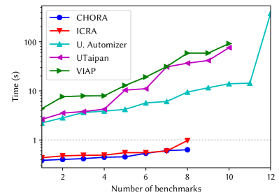
Next, we tested CHORA’s invariant-generation abilities on assertion-checking benchmarks. A standard benchmark suite from the literature is the Software Verification Competition (SV-COMP), which includes a recursive sub-category (ReachSafety-Recursive). Within this sub-category, we selected the benchmarks in the recursive sub-directory that contained true assertions, yielding a set of 17 benchmarks. We ran CHORA, ICRA, and the top three performers on this category from the 2019 competition: Ultimate Automizer (UA) (Heizmann et al., 2013), UTaipan (Dietsch et al., 2018), and VIAP (Rajkhowa and Lin, 2017). Fig. 3 presents a cactus plot showing the number of benchmarks proved by each tool, as well as the timing characteristics of their runs.

Timings were taken on a virtual machine running Ubuntu 18.04 with 16 GB of RAM, on a host machine with 32GB of RAM and a 3.7 GHz Intel i7-8000K CPU. These results demonstrate that CHORA is roughly an order of magnitude faster for each benchmark than the other tools. UA proved the assertions in 12 out of 17 benchmarks; UTaipan and VIAP each proved the assertions in 10 benchmarks; CHORA proved the assertions in 8 benchmarks; all other tools from the competition proved the assertions in 6 or fewer benchmarks.

$${\small\begin{array}[]{l}\textrm{int}~{}\textit{ackermann}(\textrm{int}~{}m,\textrm{int}~{}n)~{}\{\\ \hskip 14.22636pt\textbf{if}~{}(m==0)~{}\{~{}\textbf{return}~{}n+1;\}\\ \hskip 14.22636pt\textbf{if}~{}(n==0)~{}\{~{}\textbf{return}~{}\textit{ackermann}(m-1,1);\}\\ \hskip 14.22636pt\textbf{return}~{}\textit{ackermann}(m-1,\textit{ackermann}(m,n-1));\\ \}\\ \textit{assert}(n<0~{}||~{}m<0~{}||~{}\textit{ackermann}(m,n)>=0)\\ \hline\cr\textrm{int}~{}\textit{hanoi}(\textrm{int}~{}n)~{}\{\\ \hskip 14.22636pt\textbf{if}~{}(n==1)~{}\{~{}\textbf{return}~{}1;\}\\ \hskip 14.22636pt\textbf{return}~{}2*(\textit{hanoi}(n-1))+1;\\ \}\\ \textrm{void}~{}\textit{applyHanoi}(\textrm{int}~{}n,\textrm{int}~{}from,\textrm{int}~{}to,\textrm{int}~{}via)~{}\{\\ \hskip 14.22636pt\textbf{if}~{}(n==0)~{}\{~{}\textbf{return};\}\\ \hskip 14.22636ptcounter\texttt{++};\\ \hskip 14.22636pt\textit{applyHanoi}(n-1,from,via,to);\\ \hskip 14.22636pt\textit{applyHanoi}(n-1,via,to,from);\\ \}\\ counter=0;\textit{applyHanoi}(n,...);~{}\textit{assert}(\textit{hanoi}(n)==counter)\\ \hline\cr\textrm{int}~{}\textit{f91}(\textrm{int}~{}\textit{x})~{}\{\\ \hskip 14.22636pt\textbf{if}~{}(x>100)~{}\textit{return}~{}x-10;\textbf{else}~{}\{~{}\textit{return}~{}\textit{f91}(\textit{f91}(x+11))~{}\};\\ \}\\ res=f91(x);\textit{assert}(res==91~{}||~{}x>101~{}\&\&~{}res==x-10)\\ \end{array}}$$

Figure 4. Source code for three programs from the SV-COMP suite: Ackermann01, RecHanoi01, and McCarthy91

While the SV-COMP benchmarks do give some insight into CHORA’s invariant-generation capability, the recursive suite is not an ideal test of that capability, because the suite contains many benchmarks that can be proved safe by unrolling (e.g., verifying that Ackermann’s function evaluated at (2,2) is equal to 7). That is, many of these benchmarks do not actually require an analyzer to perform invariant generation.

We now discuss three benchmarks from the SV-COMP suite that do give some insight into CHORA’s capabilities, in that they are non-linearly recursive benchmarks that require an analyzer to perform invariant-generation. The Ackermann01 benchmark contains an implementation of the two-argument Ackermann function, and the benchmark asserts that the return value of Ackermann is non-negative if its arguments are non-negative; CHORA is able to prove that this assertion holds. The RecHanoi01 benchmark contains a non-linearly recursive cost-model of the Tower of Hanoi problem, along with a linearly recursive function that doubles its return value and adds one at each recursive call. The assertion in recHanoi01 states that these two functions compute the same value, and CHORA is able to prove this assertion. (The other tools that we tested, namely ICRA, UA, UTaipain, and VIAP, were not able to prove this assertion.) The McCarthy91 benchmark contains an implementation of McCarthy’s 91 function, along with an assertion that the return value of that function, when applied to an argument $x$, either (1) equals 91, or else (2) equals $x-10$. CHORA is not well-suited to prove this assertion because the asserted property is a disjunction, i.e., it describes the return value using two cases, whereas the hypothetical summaries used by CHORA do not contain disjunctions. (ICRA, UA, UTaipan, and VIAP were all able to prove this assertion.)

To further test CHORA’s capabilities, we also manually created three new assertion-checking benchmarks, shown in Fig. 5. Because our goal is to assess CHORA’s ability to synthesize invariants, our additional suite consists of recursive examples for which unrolling is an impractical strategy.

$${\small\begin{array}[]{l}\textrm{int}~{}\textit{quad}(\textrm{int}~{}m)~{}\{\\ \hskip 14.22636pt\textbf{if}~{}(m==0)~{}\{~{}\textbf{return}~{}0;\}\\ \hskip 14.22636pt\textrm{int}~{}\textit{retval};\\ \hskip 14.22636pt\textbf{do}~{}\{~{}\textit{retval}=\textit{quad}(m-1)+m~{}\}~{}\textbf{while}(*);\\ \hskip 14.22636pt\textbf{return}~{}\textit{retval};\\ \}\\ \textit{assert}(\textit{quad}(n)*2==n+n*n)\\ \hline\cr\textrm{int}~{}\textit{pow2\_overflow}(\textrm{int}~{}p)~{}\{\\ \hskip 14.22636pt\textit{// {pow2\_overflow} is called with $0\leq p\leq 29$}\\ \hskip 14.22636pt\textbf{if}~{}(p==0)~{}\{~{}\textbf{return}~{}1;\}\\ \hskip 14.22636pt\textrm{int}~{}\textit{r1}=\textit{pow2\_overflow}(p-1);\\ \hskip 14.22636pt\textrm{int}~{}\textit{r2}=\textit{pow2\_overflow}(p-1);\\ \hskip 14.22636pt\textit{assert}(\textit{r1}+\textit{r2}<1073741824);\\ \hskip 14.22636pt\textbf{return}~{}\textit{r1}+\textit{r2};\\ \}\\ \hline\cr\textrm{int}~{}\textit{height}(\textrm{int}~{}\textit{size})~{}\{\\ \hskip 14.22636pt\textbf{if}~{}(\textit{size}==0)~{}\{~{}\textbf{return}~{}0;\}\\ \hskip 14.22636pt\textrm{int}~{}\textit{left\_size}=\textit{nondet}(0,\textit{size});~{}//~{}0\leq\textit{left\_size}<\textit{size}\\ \hskip 14.22636pt\textrm{int}~{}\textit{right\_size}=\textit{size}-\textit{left\_size}-1;\\ \hskip 14.22636pt\textrm{int}~{}\textit{left\_height}=\textit{height}(\textit{left\_size});\\ \hskip 14.22636pt\textrm{int}~{}\textit{right\_height}=\textit{height}(\textit{right\_size});\\ \hskip 14.22636pt\textbf{return}~{}1+\textit{max}(\textit{left\_height},\textit{right\_height});\\ \}\\ \textit{assert}(height(n)\leq n)\\ \end{array}}$$

Figure 5. Source code for three non-linearly recursive programs containing assertions.

quad has a recursive call in a loop that may run for arbitrarily many iterations, and its return value is always $\texttt{n}(\texttt{n}+1)/2$. pow2_overflow contains an assertion inside a non-linearly recursive function, and an assumption about the range of parameter values; if the assertion passes, we may conclude that the program is safe from numerical-overflow bugs. The benchmark height asserts that the size (i.e., the number of nodes) of a tree of recursive calls is an upper bound on the height of the tree of recursive calls.

Table 2. Five analysis tools, along with the results of assertion-checking experiments using the benchmarks shown in Fig. 5. A $\checkmark$ indicates that the tool was able to prove the assertion within 900 seconds, and an X indicates that it was not. We also show the time required to analyze each benchmark.

Benchmark	CHORA	ICRA	UA	UTaipan	VIAP
quad	✓(0.70s)	✓(1.08s)	X(900s)	✓(4.24s)	X(4.71s)
pow2_overflow	✓(0.61s)	✓(1.28s)	X(900s)	X(900s)	X(1.79s)
height	✓(0.58s)	X(0.52s)	✓(8.82s)	✓(13.0s)	X(2.85s)

The results of our experiments are shown in Tab. 2. CHORA is able to prove the assertions in all three programs; ICRA and UTaipan each prove two; UA proves one, and VIAP proves none. Times taken by each tool are also shown in the table. CHORA’s ability to prove the assertion in quad illustrates that it can find invariants even for programs in which running time (and the number of recursive calls) is unbounded. quad illustrates CHORA’s applicability to perform program-equivalence tasks on numerical programs, while pow2_overflow illustrates CHORA’s applicability to perform overflow-checking.

Conclusions.

Our main experimental question is whether CHORA is effective at the problem of generating invariants for programs using non-linear recursion. Results from the complexity-analysis and assertion-checking experiment show that CHORA is able to generate non-linear invariants that are sufficient to solve these kinds of problems. In these ways, CHORA has shown success in a domain, i.e., invariant generation for non-linearly recursive programs, that is not addressed by many other tools.

6. Related Work

Following the seminal work of Cousot and Cousot (Cousot and Cousot, 1977), most invariant-generation techniques are based on iterative fixpoint computation, which over-approximates Kleene-iteration within some abstract domain. This paper presents a non-iterative method for generating numerical invariants for recursive procedures, which is based on extracting and solving recurrence relations. It was inspired by two streams of ideas found in prior work.

Template-based methods fix a desired template for the invariants in a program, in which there are undetermined constant symbols (Colón et al., 2003; Sankaranarayanan et al., 2004a). Constraints on the constants are derived from the structure of the program, which are given to a constraint solver to derive values for the constants. The hypothetical summaries introduced in §4.1 were inspired by template-based methods, but go beyond them in an important way: in particular, the indeterminates in a hypothetical summary are functions rather than constants, and our work uses recurrence solving to synthesize these functions.

Of particular relevance to our work are template-based methods for generating non-linear invariants (Kapur, 2004; Sankaranarayanan et al., 2004b; Cachera et al., 2012; Kojima et al., 2016; Chatterjee et al., 2019). Contrasting with the technique proposed in this paper, a distinct advantage of template-based methods for generating polynomial invariants for programs with real-typed variables is that they enjoy completeness guarantees (Kapur, 2004; Sankaranarayanan et al., 2004b; Chatterjee et al., 2019), owing to the decidability of the theory of the reals. The advantages of our proposed technique over traditional template-based techniques are (1) it is compositional, (2) it can generate exponential and logarithmic invariants, and (3) it does not require fixing bounds on polynomial degrees a priori. Also note that template-based techniques pay an up-front cost for instantiating templates that is exponential in the degree bound. (In practice, this exponential blow-up can be mitigated (Kojima et al., 2016).)

Recurrence-based methods find loop invariants by extracting recurrence relations between the pre-state and post-state of the loop and then generating invariants from their closed forms (Farzan and Kincaid, 2015; Kincaid et al., 2018, 2019; Rodríguez-Carbonell and Kapur, 2004; Humenberger et al., 2017; Kovács, 2008; de Oliveira et al., 2016; Humenberger et al., 2018). This paper gives an answer to the question of how such analyses can be applied to recursive procedures rather than loops, by extracting height-indexed recurrences using template-based techniques.

Reps et al. (2017) demonstrate that tensor products can be used to apply loop analyses to linearly recursive procedures. This technique is used in the recurrence-based invariant generator ICRA to handle linear recursion (Kincaid et al., 2017). ICRA falls back on a fixpoint procedure for non-linear recursion; in contrast, the technique presented in this paper uses recurrence solving to analyze recursive procedures.

Rajkhowa and Lin (2017) presents a verification technique that analyzes recursive procedures by encoding them into first-order logic; recurrences are extracted and replaced with closed forms as a simplification step before passing the query to a theorem prover. In contrast to this paper, Rajkhowa and Lin (2017)’s approach has the flexibility to use other approaches (e.g., induction) when recurrence-based simplification fails, but cannot be used for general-purpose invariant generation.

Resource-bound analysis (Wegbreit, 1975) is another related area of research. Three lines of recent research in resource-bound analysis are represented by the tools PUBS (Albert et al., 2011), CoFloCo (Flores Montoya, 2017), KoAT (Brockschmidt et al., 2016), and RAML (Hoffmann et al., 2012). In resource-bound analysis, the goal is to find an expression that upper-bounds or lower-bounds the amount of some resource (e.g., time, memory, etc.) used by a program. Resource-bound analysis typically consists of two parts: (i) size analysis, which finds invariants that bound program variables, and (ii) cost analysis, which finds bounds on cost using the results of the size analysis. Cost can be seen as an auxiliary program variable, although it is updated in a restricted manner (by addition only), it has no effect on control flow, and it is often assumed to be non-negative. Our work differs from resource-bound analyzers in several ways, ultimately because our goal is to find invariants and check assertions, rather than to find resource bounds specifically.

The capabilities of our technique are different, in that we are able to find non-linear mathematical relationships (including polynomials, exponentials, and logarithms) between variables, even in non-linearly recursive procedures. PUBS and CoFloCo use polyhedra to represent invariants, so they are restricted to finding linear relationships between variables, although they can prove that programs have non-linear costs. KoAT has the ability to find non-linear (polynomial and exponential) bounds on the values of variables, but it has limited support for analyzing non-linearly recursive functions; in particular, KoAT cannot reason about the transformation of program state performed by a call to a non-linearly recursive function. Typically, resource-bound analyzers also reason about non-terminating executions of a program, whereas our analysis does not. RAML reasons about manipulations of data structures, whereas our work only reasons about integer variables. Originally, RAML only discovered polynomial bounds, although recent work (Kahn and Hoffmann, 2019) extends the technique to find exponential bounds.

The algorithms that we use are different in that we have a unified approach, rather than separate approaches, for analyzing cost and analyzing a program’s transformation of other variables. To perform resource-bound analysis, we materialize cost as a program variable and then find a procedure summary; the summary describes the program’s transformation of all variables, including the cost variable. Recurrence-solving is the essential tool that we use for analyzing loops, linear recursion, and non-linear recursion, and we are able to find non-linear mathematical relationships because such relationships arise in the solutions of recurrences.

Appendix A Appendix

In this section, we provide a detailed argument for the soundness of height-based recurrence analysis. We discuss the process of performing a height-based recurrence analysis on some procedure $P$. The sequence of operations in that analysis is as follows. First, Alg. 2 analyzes $P$, and produces as output a set of candidate recurrence inequations. On lines (2)–(2), Alg. 2 also produces a set $\{\tau_{i}\}_{i\in[1,n]}$ of two-vocabulary relational expressions. Next, Alg. 3 filters down the set of candidate recurrences produced by Alg. 2 to obtain a stratified recurrence that can be solved by a C-finite recurrence solver. Finally, a recurrence solver produces a solution in the form of a set of functions $\{b_{i}\}_{i\in B}$, where $B=\{i_{1},...,i_{m}\}$ is a subset of the indices $[1,n]$.

In this discussion of soundness, we wish to relate the functions $\{b_{i}\}_{i\in B}$ that are produced by the analysis to the sets of values $V_{\tau}(P,h)$ taken on by each relational expression $\tau_{i}$ at each height $h$, which have the following definition in terms of the relational semantics given in §3:

$$V_{\tau}(P,h)\buildrel\mbox{\tiny\rm def}\over{=}\{\mathcal{E}\llbracket\tau\rrbracket(\sigma,\sigma^{\prime}):(\sigma,\sigma^{\prime})\in R(P,h)\}.$$

We use $V_{\tau}(P,h)$ to prove a height-relative soundness property of our procedure summaries, which contain the height $h$ as an explicit parameter. The fact that the summaries contain an explicit representation of height means that they can be made more precise by conjoining them to the depth-bound summaries computed in §4.2.

The goal of this section is to prove the following soundness theorem.

Theorem A.1.

Let $P$ be a procedure to which Alg. 2 and Alg. 3 have been applied to obtain stratified recurrence. Let $\{\tau_{i}\}_{i\in[1,n]}$ be the relational expressions computed by Alg. 2. Let $B\subseteq[1,n]$ be such that $\{b_{i}\}_{i\in B}$ is the set of functions produced by solving the stratified recurrence. Then, the following statement holds: $\forall h\geq 1.\bigwedge_{i\in B}\forall v\in V_{\tau_{i}}(P,h).v\leq b_{i}(h)$.

We will prove Thm. A.1 by induction on the height $h$. However, before the main inductive argument, we will provide some definitions, and discuss the properties of Alg. 2, the recurrence-extraction algorithm Alg. 3, and the set of functions $\{b_{i}\}_{i\in B}$. (Note that the Alg. 3 referred to in this appendix is not the same as the Alg. 3 that appears in the conference version (Breck et al., 2020b) of this document, which appears as the depth-bounding algorithm Alg. 4 in this technical report version.)

Define a feasible trace of a procedure $P$ to be a finite list of pairs of control locations and program states, starting at the entry location of $P$, ending at the exit location of $P$, in which all the state transitions are consistent with the semantics of $P$, and all calls are matched by returns. Note that this definition only considers finite (i.e., terminating) traces of $P$, which is useful because our ultimate goal is to find procedure summaries that over-approximate a procedure’s pre-state-post-state relation, and a procedure only has a post-state when it terminates. (As described below, we will also discuss a modified version of $P$ called $\hat{P}$, and we will consider the feasible traces of $\hat{P}$ to be only those that meet some additional constraints.) Furthermore, we define the feasible traces of $P$ up to height $h$ to be those feasible traces that have a recursion depth not exceeding $h$. For the following soundness proof, we define invariants of $P$ to be properties that hold in all feasible traces of $P$.

As explained above, the main function of Alg. 3 is to filter down the set of candidate recurrence inequations produced by Alg. 2, to obtain a subset that constitute a stratified recurrence. At the end of that process, the inequations are changed into equations so as to obtain the maximal solution to the set of inequations. The output of Alg. 3 is a stratified recurrence that can be written as:

$$\bigwedge_{i\in B}b_{i}(h+1)=p_{i}(b_{i_{1}}(h),\ldots,b_{i_{m}}(h)),$$

in which each $p_{i}(x_{1},\ldots,x_{m})$ is a polynomial in the variables $x_{1},\ldots,x_{m}$.

All coefficients in the polynomials $\{p_{i}\}_{i\in B}$ are non-negative, including the constant coefficients, as a result of line (3) of Alg. 3, which drops terms having negative coefficients from the polynomial inequations that are given as input to Alg. 3, thereby weakening the inequations. Aside from line (3), all other steps of Alg. 3 serve only to filter down the set of candidate recurrences. Because of the dropping of terms having negative coefficients on line (3), the polynomials $p_{i}$ may differ from the corresponding polynomials that appeared in the input to Alg. 3; for each $i\in B$, we denote by $p_{i}^{\prime}$ the corresponding polynomial in the input, before terms having negative coefficients were dropped. We refer to the candidate inequations involving the $p_{i}^{\prime}$ polynomials as the selected candidate inequations, because they are the ones that are selected by Alg. 3 for inclusion in the stratified recurrence (after their terms having negative coefficients are dropped).

During the recurrence-solving phase, the zero vector is used as the initial condition of the recurrence. Thus, the set of functions that occur as the solution to the recurrence satisfy $\forall i\in B,b_{i}(1)=0$. Because all polynomials $p_{i}$ have only non-negative coefficients, the functions $\{b_{i}(h)\}_{i\in B}$ are non-negative and non-decreasing for $h\geq 1$.

Our final digression before proving Thm. A.1 is a discussion of Alg. 2. Alg. 2 operates by manipulating formulas that include a set of function symbols named $\{b_{i}(h)\}_{i\in[1,n]}$ and $\{b_{i}(h+1)\}_{i\in[1,n]}$. The names of these symbols are the same as those of the corresponding functions that are derived by recurrence solving; however, in this proof, we will use separate names for the symbols manipulated by Alg. 2 and the corresponding functions. Instead of $b_{i}(h)$ we will refer to the symbol $x_{i}$, and instead of $b_{i}(h+1)$, we will refer to the symbol $y_{i}$. Furthermore, although Alg. 2, as written, manipulates formulas that are augmented with these additional symbols, it will be convenient in the following argument to take an alternative, but equivalent, view, according to which Alg. 2 analyzes a modified version of the procedure $P$ called $\hat{P}$ that is obtained by making three changes to $P$.

First, $\hat{P}$ is augmented with a set of immutable auxiliary variables named $x_{1},...,x_{n},y_{1},...,y_{n}$. Second, we impose a constraint on the feasible traces of $\hat{P}$, namely that the pre-state $\sigma$ and post-state $\sigma^{\prime}$ of any trace $t$ of $\hat{P}$ must satisfy the constraint $\bigwedge_{i=1}^{n}(y_{i}=\mathcal{E}\llbracket\tau_{i}\rrbracket(\sigma,\sigma^{\prime}))$, or else $t$ is not considered to be a feasible trace of $\hat{P}$. This constraint is the equivalent of the formula-manipulation performed by line (2) of Alg. 2.

Third, the recursive call sites in $P$ are replaced with control-flow edges that havoc their post-state $\sigma^{\prime}$ and execute $\textit{assume}(\varphi_{\textit{call}})$. That is, the feasible executions of these control-flow edges of $\hat{P}$ are all those in which the pre-state $\sigma$ and post-state $\sigma^{\prime}$ of the control-flow edge satisfy $\bigwedge_{i=1}^{n}(\mathcal{E}\llbracket\tau_{i}\rrbracket(\sigma,\sigma^{\prime})\leq x_{i}\land x_{i}\geq 0)$. The effect of replacing call edges of $P$ in this way is equivalent to that of the formula-manipulation performed by line (2) of Alg. 2.

Having described the above constraints on feasible executions of $\hat{P}$, we can now succinctly describe the output of Alg. 2: each of the candidate recurrence inequations returned by Alg. 2 is an invariant of $\hat{P}$, i.e., a property that holds in all feasible executions of $\hat{P}$. The soundness of these invariants follows from the soundness of the underlying program-analysis primitives used by Alg. 2. For the proof of Thm. A.1, the crucial invariant of $\hat{P}$ is the conjunction of the selected candidate inequations:

(18) $$\{y_{i}\leq p_{i}^{\prime}(x_{i_{1}},...,x_{i_{m}})\}_{i\in B}.$$

We now begin the inductive proof of Thm. A.1.

Proof.

The base case of the proof corresponds to a height value of 1, which in turn corresponds to executions of the base case of procedure $P$. At height 1, we must show:

$$\bigwedge_{i\in B}\forall v\in V_{\tau_{i}}(P,1).v\leq b_{i}(1),$$

which holds because each relational expression $\tau_{i}$ was constructed to be bounded above by zero in the base case, and each bounding function $b_{i}$ evaluates to zero at height 1.

The inductive step of the proof is as follows. The inductive hypothesis states that, for some $h$,

$$\bigwedge_{i\in B}\forall v\in V_{\tau_{i}}(P,h).v\leq b_{i}(h),$$

and the goal is to prove that

$$\bigwedge_{i\in B}\forall v\in V_{\tau_{i}}(P,h+1).v\leq b_{i}(h+1).$$

Let $t$ be any feasible trace of $P$ at height up to $h+1$. We will show that we can modify the trace $t$ to produce a new trace $\hat{t}$, and we then prove that $\hat{t}$ is a feasible trace of $\hat{P}$.

To construct $\hat{t}$, first modify $t$ to add the immutable auxiliary variables $x_{1},...,x_{m},y_{1},...,y_{m}$ to each program state in $t$. We choose the values of these auxiliary variables as follows. Let $\sigma$ and $\sigma^{\prime}$ be, respectively, the initial and final states of $t$. For each $i\in[1,n]$, set $y_{i}$ to be the result of evaluating the relational expression $\tau_{i}$ using the state pair $(\sigma,\sigma^{\prime})$, that is, $y_{i}=\mathcal{E}\llbracket\tau_{i}\rrbracket(\sigma,\sigma^{\prime})$. Define the outermost recursive calls in the feasible trace $t$ to be the recursive calls to $P$ that do not occur inside any other recursive call to $P$. Any feasible trace $t$ is of finite length, and therefore $t$ contains some finite number of outermost recursive calls. Thus, the set $R_{i,t}$ of values taken on by $\tau_{i}$ evaluated at the pre-state/post-state pairs of each outermost recursive call in $t$ is a finite set, and therefore we may define $M_{i,t}\overset{\underset{\text{def}}{}}{=}\max(0,\max(R_{i,t}))$ to be the maximum value of $\tau_{i}$ occurring at any outermost recursive call in $t$. Now set each of the auxiliary variables $x_{i}$ as follows:

$$x_{i}=\begin{cases}b_{i}(h)&\text{if}~{}i\in B\\ M_{i,t}&\text{otherwise}\end{cases}$$

Finally, modify $\hat{t}$ by collapsing all of the intermediate steps of each outermost recursive call in $t$ into a single state transition, so as to match the replacement of recursive-call edges of $P$ with their corresponding edges in $\hat{P}$.

We now argue that $\hat{t}$ meets all the necessary constraints to be considered a feasible trace of $\hat{P}$. The constraint on the initial and final state of $\hat{t}$ is that $\bigwedge_{i=1}^{n}(y_{i}=\tau_{i})$, which holds by construction. The constraint at each outermost recursive call of $t$ is that, if $(\sigma,\sigma^{\prime})$ are, respectively, the pre-state and the post-state of the call, then $\bigwedge_{i=1}^{n}(\mathcal{E}\llbracket\tau_{i}\rrbracket(\sigma,\sigma^{\prime})\leq x_{i}\land x_{i}\geq 0)$. For $i\notin B$, $x_{i}=M_{i,t}$, and each such $M_{i,t}$ satisfies the constraint by construction.

For $i\in B$, $x_{i}=b_{i}(h)$. We must show that $x_{i}$ is greater than or equal to $\mathcal{E}\llbracket\tau_{i}\rrbracket(\sigma,\sigma^{\prime})$ and also greater than or equal to zero. Each $x_{i}$ is non-negative because each $b_{i}(h)$ is non-negative. By hypothesis, $t$ is a feasible execution trace of $P$ at height $h+1$. Thus, each outermost recursive call in $t$ corresponds to an execution of $P$ of height at most $h$. (Note that, if a trace is at height exactly $h+1$, one of its recursive calls must be at height exactly $h$, but the others may be at any height between 1 and $h$ (inclusive).) Thus, the inductive hypothesis,

$$\bigwedge_{i\in B}\forall v\in V_{\tau_{i}}(P,h).v\leq b_{i}(h),$$

implies that the constraint relating $x_{i}$ to the value of $\tau_{i}$ is met at each call. We conclude that the relevant constraints on $\hat{t}$ are met, and therefore $\hat{t}$ is a feasible trace of $\hat{P}$.

As noted above, the output Alg. 2 is a set of invariants of $\hat{P}$, i.e., properties that hold in all feasible traces of $\hat{P}$. One such property is the conjunction of the selected candidate inequations shown in Eqn. (18). Let $i\in B$. We conclude that the $i^{\textrm{th}}$ selected candidate inequation holds in $\hat{t}$:

$$y_{i}\leq p_{i}^{\prime}(x_{i_{1}},...,x_{i_{m}})$$

Let $\sigma$ and $\sigma^{\prime}$ be the initial and final states of $\hat{t}$. By the construction of $\hat{t}$, we know that $\mathcal{E}\llbracket\tau_{i}\rrbracket(\sigma,\sigma^{\prime})=y_{i}$. Thus,

$$\mathcal{E}\llbracket\tau_{i}\rrbracket(\sigma,\sigma^{\prime})\leq p_{i}^{\prime}(x_{i_{1}},...,x_{i_{m}})$$

By the construction of $\hat{t}$, we know that, for each $k\in B$, $x_{k}=b_{k}(h)$. Thus,

$$\mathcal{E}\llbracket\tau_{i}\rrbracket(\sigma,\sigma^{\prime})\leq p_{i}^{\prime}(b_{i_{1}}(h),...,b_{i_{m}}(h))$$

As noted above, each $b_{i}(h)$ is non-negative for any $h\geq 1$. Thus, because $p_{i}^{\prime}$ and $p_{i}$ are being evaluated at non-negative arguments, and $p_{i}$ was derived from $p_{i}^{\prime}$ by dropping negative coefficients, we conclude that $p_{i}^{\prime}(b_{i_{1}}(h),...,b_{i_{m}}(h))\leq p_{i}(b_{i_{1}}(h),...,b_{i_{m}}(h))$ and therefore,

(19) $$\mathcal{E}\llbracket\tau_{i}\rrbracket(\sigma,\sigma^{\prime})\leq p_{i}(b_{i_{1}}(h),...,b_{i_{m}}(h)).$$

The right-hand side Eqn. (19) matches the right-hand side of the defining recurrence for $b_{i}$, i.e., $p_{i}(b_{i_{1}}(h),...,b_{i_{m}}(h))=b_{i}(h+1)$. Thus,

$$\mathcal{E}\llbracket\tau_{i}\rrbracket(\sigma,\sigma^{\prime})\leq b_{i}(h+1).$$

Because we have shown this inequation to hold for each $i\in B$, we conclude that

(20) $$\bigwedge_{i\in B}\mathcal{E}\llbracket\tau_{i}\rrbracket(\sigma,\sigma^{\prime})\leq b_{i}(h+1).$$

Recall that $\sigma$ and $\sigma^{\prime}$ are the initial and final states of $\hat{t}$, and that, by the construction of $\hat{t}$, these are also the initial and final states of the original trace $t$ of $P$. But $t$ was an arbitrary feasible execution trace of $P$ of height up to $h+1$, and therefore we conclude that Eqn. (20) holds if $(\sigma,\sigma^{\prime})$ are the initial and final states of any feasible execution trace of $P$ of height up to $h+1$. Thus,

$$\bigwedge_{i\in B}\forall v\in V_{\tau_{i}}(P,h+1).v\leq b_{i}(h+1),$$

and the proof is complete. ∎