Nonlinearity and discreteness: solitons in lattices

Abstract

An overview is given of basic models combining discreteness in their linear parts (i.e., the models are built as dynamical lattices) and nonlinearity acting at sites of the lattices or between the sites. The considered systems include the Toda and Frenkel-Kontorova lattices (including their dissipative versions), as well as equations of the discrete nonlinear Schrödinger and Ablowitz-Ladik types, and their combination in the form of the Salerno model. The interplay of discreteness and nonlinearity gives rise to a variety of states, most important ones being discrete solitons. Basic results for 1D and 2D discrete solitons are collected in the review, including 2D solitons with embedded vorticity, and some results concerning mobility of discrete solitons.Main experimental findings are overviewed too. Models of the semi-discrete type, and basic results for solitons supported by them, are also considered, in a brief form. Perspectives for the development of topics covered the review are discussed throughout the text.

I Introduction: discretization of continuum models, and the continuum limit of discrete ones

Standard models of dynamical media are based on partial differential equations, typical examples being the nonlinear Schrödinger (NLS) equation for the mean-field complex wave function $\psi\left(x,y,z.t\right)$ in atomic Bose-Einstein condensates (BECs; in that case, the NLS equation is usually called the Gross-Pitaevskii equation (GPE) Pethick ), and the NLS equation for the envelope amplitude of the electromagnetic field in optical media Gadi . In the scaled form, the NLS equation is

$$i\psi_{t}=-(1/2)\nabla^{2}\psi+g|\psi|^{2}\psi+U\left(x,y,z\right)\psi,$$ (1)

where $g=+1$ and $-1$ correspond to the self-defocusing and focusing signs of the local cubic nonlinearity, and $U\left(x,y,z\right)$ is a real external potential. In the application to optics, the evolution variable $t$ is replaced by coordinate $z$ in the propagation direction, while original $z$ is replaced by the temporal variable, $\tau=t-z/V_{\mathrm{gr}}$, where $t$ is time, and $V_{\mathrm{gr}}$ is the group velocity of the carrier wave KA . In optics, the effective potential may be two-dimensional (2D), $-U(x,y)$ being a local variation of the refractive index in the transverse plane.

In many cases the potential represents a spatially periodic pattern, such as optical lattices (OLs) in BEC OL ; Porter , or photonic crystals which steer the propagation of light waves PhotCryst in optics:

$$U_{\mathrm{latt}}\left(x,y,z\right)=-\varepsilon\left[\cos(2\pi L/x)+\cos(2\pi L/y)+\cos(2\pi L/z)\right],$$ (2)

as well as its 2D and 1D reductions. A deep lattice potential, which corresponds to large $\varepsilon$, splits the continuous wave function into an array of “droplets” trapped in local potential wells, which are coupled by weak tunneling. Accordingly, in the framework of the tight-binding approximation, the NLS equation is replaced by a discrete NLS (DNLS) equation, which was derived, in the 1D form, for arrays of optical fibers ChristoJoseph ; Silberberg ; discr-review-0 ; discr-review and arrays of plasmonic nanowires Nicolae , as well as for BEC loaded in a deep OL trap Smerzi :

$$i\dot{\psi}_{l,m,n}=-(1/2)\left[\left(u_{l+1,m,n}+\psi_{l-1,m,n}-2\psi_{l,m,n}\right)+\left(\psi_{l,m+1,n}+\psi_{l,m-1,n}-2\psi_{l,m,n}\right)\right.$$

$$\left.+\left(\psi_{l,m,n+1}+\psi_{l,m,n-1}-2\psi_{l,m,n}\right)\right]+g\left|\psi_{l,m,n}\right|^{2}\psi_{l,m.n},$$ (3)

where the set of integer indices, $\left(l,m,n\right)$, replaces coordinates $\left(x,y,z\right)$. DNLS equation (3) is often reduced to 2D and 1D forms. While it includes the linear coupling between the nearest neighbors, 1D lattices can be built in the form of zigzag chains, making it relevant to add couplings between the next-nearest neighbors NNN ; ChongNNN . 2D lattices with similar additional coupling are known too NNN2D .

As concerns the sign parameter, $g=\pm 1$, Eq. (3) admits flipping $+1\leftrightarrow-1$ by means of the staggering transformation of the discrete wave function:

$$\psi_{l,m,n}(t)\equiv(-1)^{l+m+n}\exp\left(-6it\right)\tilde{\psi}_{l,m,n}^{\ast}(t)$$ (4)

where $\ast$ stands for the complex-conjugate expression, and (in the 2D and 1D situations, $\exp\left(-6it\right)$ is replaced by $\exp\left(-4it\right)$ and $\exp\left(-2it\right)$, respectively).

It is well known that the 2D and 3D continuous NLS equation (1) with the self-focusing nonlinearity, i.e. $g<0$, gives rise to the critical and supercritical collapse, respectively, i.e., appearance of singular solutions in the form of infinitely narrow and infinitely tall peaks, after a finite evolution time Gadi . The discreteness arrests the collapse, replacing it by a quasi-collapse Laedke , when the width of the shrinking peak becomes comparable to the spacing of the DNLS lattice.

The DNLS equation and its extensions constitute a class of models with a large number of physical realizations, which have drawn much interest as subjects of mathematical studies as well DNLS-book . The class also includes systems of coupled DNLS equations Angelis ; Herring .

The 1D continuous NLS equation without the external potential and with either sign of the nonlinearity, $g$, is integrable by means of the inverse-scattering transform Zakh ; Segur ; Calogero ; Newell , although it is nonintegrable in the 2D and 3D geometries. On the contrary to that, the 1D DNLS equation is not integrable, i.e., the direct discretization destroys the integrability Herbst ; non-integrable . However, the continuous NLS equation admits another discretization in 1D, which leads to an integrable discrete model, viz., the Ablowitz-Ladik (AL) equation AL :

$$i\dot{\psi}_{n}=-\left(\psi_{n+1}+\psi_{n-1}\right)\left(1+\mu\left|\psi_{n}\right|^{2}\right),$$ (5)

where positive and negative values of the real nonlinearity coefficient, $\mu$, correspond to the self-focusing and defocusing, respectively. Considerable interest was also drawn to the nonintegrable combination of the AL and DNLS equations, in the form of the Salerno model (SM) SA , with an additional onsite cubic term, different from the intersite one in (5):

$$i\dot{\psi}_{n}=-\left(\psi_{n+1}+\psi_{n-1}\right)\left(1+\mu\left|\psi_{n}\right|^{2}\right)-2\left|\psi_{n}\right|^{2}\psi_{n},$$ (6)

with the magnitude and sign of the onsite nonlinearity coefficient fixed by means of the rescaling and staggering transformation, respectively. The SM finds a physical realization in the context of the Bose-Hubbard model, i.e., BEC loaded in a deep OL, in the case when dependence of the intersite hopping rate on populations of the sites is taken into regard BH ; BH-review .

While the above-mentioned DNLS, AL, and SM discrete systems are derived as the discretization of continuous NLS equations, one can look at this relation in the opposite direction: starting from discrete equations, one can derive their continuum limit. In particular, in the case of the SM equation (6), the continuum approximation is introduced by replacing the intersite combination of the discrete fields by a truncated Taylor’s expansion,

$$\psi_{n}(t)\equiv e^{2it}\Psi(x,t),\qquad\Psi\left(x=n\pm 1,t\right)\approx\Psi\left(x=n\right)\pm\Psi_{x}{\big{|}}_{x=n}+(1/2)\Psi_{xx}{\big{|}}_{x=n},$$ (7)

where $\Psi(x)$ is treated as a function of continuous coordinate $x$, which coincides with $n$ when it takes integer values. The substitution of this approximation in (6) leads to a generalized (nonintegrable) form of the 1D NLS equation Zaragoza

$$i\Psi_{t}=-\left(1+\mu\left|\Psi\right|^{2}\right)\Psi_{xx}-2\left(1+\mu\right)\left|\Psi\right|^{2}\Psi,$$ (8)

which goes over into the standard 1D NLS equation (1) with $g=+1$ and $U=0$ in the case of $\mu=0$.

The objective of this Chapter is to present an overview of basic discrete nonlinear models and dynamical states produced by them, chiefly in the form of bright solitons (self-trapped localized modes). Before proceeding to models based on equations of the DNLS, AL, and SM types, simpler ones, which were derived for chains of interacting particles, are considered in the next section. The paradigmatic model of the latter type is provided by the 1D Toda-lattice (TL) equation Toda , written for coordinates $u_{n}(t)$ of particles with unit mass and exponential potential of interaction between adjacent ones:

$$\ddot{u}_{n}+\,e^{-\left(u_{n+1}-u_{n}\right)}-e^{-\left(u_{n}-u_{n-1}\right)}=0.$$ (9)

This equation can also be written for separations $r_{n}(t)\equiv u_{n+1}(t)-u_{n}(t)$ between the particles:

$$\ddot{r}_{n}+\,e^{-r_{n+1}}+e^{-r_{n-1}}-\,2e^{-r_{n}}=0.$$ (10)

Equation (10) is integrable Zakh , its continuum limit being the so-called “bad” Boussinesq equation Johnson , which is formally integrable too Calogero :

$$r_{tt}-r_{xx}-(1/12)r_{xxxx}+\left(r^{2}\right)_{xx}=0$$ (11)

Another famous, although not integrable, model of a chain of pairwise-interacting particles with coordinates $u_{n}(t)$, is the Fermi-Pasta-Ulam (FPU) system FPU ; FPU2 :

$$\ddot{u}_{n}=\left(u_{n+1}+u_{n-1}-2u_{n}\right)\left[1+\alpha\left(u_{n+1}-u_{n-1}\right)\right],$$ (12)

where $\alpha$ is a constant. This model was one of the first objects of numerical simulations performed in the context of fundamental research (in 1953, published in 1955 FPU , see also FPU3 ). Later, it became known that a very essential contribution to the original FPU work was made by Mary Tsingou Tsingou , therefore the model is also called the FPU-Tsingou system.

The initial objective of the original numerical FPU-Tsingou experiment was to observe the onset of ergodicity in the evolution governed by (12). A surprising result was that long simulations demonstrated a quasi-periodic evolution, without manifestations of ergodicity (i.e. without statistically uniform distribution of the energy between all degrees of freedom of the lattice system). Eventually, this perplexing result was explained (in the same paper soliton by N. Zabusky and M. Kruskal which had introduced word “soliton”) by the fact that the continuum limit of (12) may be reduced (for unidirectional propagation in excitations in the continuum medium) to the Korteweg – de Vries equation, which, being integrable, does not feature ergodicity.

The next section briefly addresses, in addition to the TL, more complex models which combine the inter-particle interactions (taken in the linear approximation, unlike the exponential terms in (10)), and onsite potentials – most typically, in the form of $U=\varepsilon\sum_{n}\left(1-\cos u_{n}\right),$ with $\varepsilon>0$, which is the source of the nonlinearity in the corresponding Frenkel-Kontorova (FK) model. It was originally introduced as a model for dislocations in a crystalline lattice FrKo , and has found a large number of realizations in other physical settings Braun

This Chapter also addresses, in a brief form, other models of nonlinear discrete systems. These are discrete multidimensional models, semi-discrete ones, and experimental realizations of discrete media and bright solitons in them, chiefly in the realm of nonlinear optics. Dissipative discrete nonlinear systems are partly addressed in this Chapter, as a systematic consideration of dissipative discrete systems is a subject for a separate review.

Because the length of the Chapter is limited, the presentation and bibliography are not aimed to be comprehensive; rather, particular results mentioned in sections following below are selected as examples which help to understand general principles supported by a large body of theoretical and experimental findings.

II Excitations in chains of interacting particles

II.1 The Toda lattice

The TL equation (9) is characterized, first of all, by its linear spectrum. Looking for solutions to the linearized version of the equation in the form of “phonon modes”, i.e. plane waves with an infinitesimal amplitude $u^{(0)}$, frequency $\chi$ and wavenumber $p$ (which is constrained to the first Brillouin zone, $0<p<2\pi$),

$$\left(u_{n}\right)_{\mathrm{linearized}}=u^{(0)}\exp\left(ipn-i\chi t\right),$$ (13)

it is easy to obtain the respective dispersion relation,

$$\chi=\pm 2\sin\left(p/2\right).$$ (14)

Further, (13) produces phase velocities of the linear waves, $V_{\mathrm{ph}}=\chi/p$, which take values $\left|V_{\mathrm{ph}}\right|<1$.

Integrable equation (9) generates exact soliton solutions, which were first found in the original work of Toda Toda . The soliton represents a lattice deformation traveling at constant velocity $c$:

$$u_{n}=-\ln\left[\xi^{-2}-\frac{\xi^{-2}-1}{1+\xi^{2(n-ct)}}\right],\quad c=\pm\frac{\xi^{-1}-\xi}{\ln\left(\xi^{-2}\right)},$$ (15)

where $\xi$ is an arbitrary real parameter taking values $0<\xi<1$, the respective interval of the inverse velocities being

$$0<|c|^{-1}<1.$$ (16)

Note that this interval has no overlap with the above-mentioned range of the phase velocities of the linear modes, $\left|V_{\mathrm{ph}}\right|<1$, in accordance with the well-known principle that solitons may exist in bandgaps of linear spectra, i.e., in regions where linear waves do not exist.

Comparing values of the solution (15) at $n\rightarrow\pm\infty$, one concludes that the soliton carries compression of the TL by a finite amount, $\Delta u\equiv u_{n=+\infty}-u_{n=-\infty}=\ln\left(\xi^{-2}\right)$, while a characteristic width of the soliton is $\Delta n\sim 1/\ln\left(\xi^{-2}\right)$. Similar to other integrable systems Zakh ; Segur ; Calogero ; Newell , collisions between solitons do not affect their shapes and velocities, leading solely to finite shifts of the solitons’ centers.

The limit of $\xi\rightarrow 0$ implies that the TL reduces to a chain of hard particles, which interact when they collide. Accordingly, the soliton’s structure degenerates into a single fast moving particle, the propagation being maintained by periodically occurring collisions, as a result of which the moving particle comes to a halt, transferring its momentum to the originally quiescent one. In the opposite limit, $\xi\rightarrow 1$, soliton (15) becomes a very broad solution, traveling with the minimum velocity, $c\rightarrow 1$. As mentioned above, no TL solitons exists with velocities $|c|<1$.

Equation (9) conserves the total momentum, $P=\sum_{-\infty}^{+\infty}\dot{u}_{n}$, and Hamiltonian (energy),

$$H_{\mathrm{TL}}=\sum_{n=-\infty}^{+\infty}\left\{\frac{1}{2}\dot{u}_{n}^{2}+\left[e^{-\left(u_{n+1}-u_{n}\right)}-1\right]\right\}.$$ (17)

In fact, integrable equations, including (9), conserve an infinite number of dynamical invariants, the momentum and energy being the lowest-order ones in the infinite sequence Zakh ; however, higher-order invariants do not have a straightforward physical interpretation.

A realistic implementation of the TL includes friction forces with coefficient $\alpha>0$, which should be compensated by an “ac” (time-periodic) driving force with amplitude $\varepsilon$ and frequency $\omega$ drivenTL ; Jarmo ; Rasmussen . The accordingly modified equation (9) is

$$\ddot{u}_{n}+\,e^{-\left(u_{n+1}-u_{n}\right)}-e^{\left(u_{n}-u_{n-1}\right)}=-\alpha\dot{u}_{n}+\varepsilon q_{n}\cos\left(\omega t\right).$$ (18)

Here coefficients $q_{n}$ may be realized as charges of the particles, if the drive is applied by an ac electric field. Nontrivial coupling of the field to the TL dynamics is not possible if all the charges are identical, i.e. $q_{n}\equiv 1$. Indeed, in the latter case one can trivially eliminate the drive by defining $u_{n}(t)\equiv v_{n}(t)-\varepsilon\omega^{-2}\cos\left(\omega t\right)$, ending up with an equation (18) for $v_{n}(t)$ with no drive. The simplest nontrivial coupling is provided by assuming $q_{n}=(-1)^{n}$, i.e. alternating positive and negative charges at neighboring sites of the TL drivenTL . A particular choice of the periodic pattern for $q_{n}$ defines the respective size, $a$, of the cell of the ac-driven TL (in particular, $q_{n}=(-1)^{n}$ corresponds to $a=2$).

The periodic passage of the soliton running through the lattice with velocity $c$, i.e., with temporal period $T=a/c$, may provide compensation of the friction losses if it resonates with the periodicity of the ac drive, which defines the spectrum of resonant velocities drivenTL ,

$$c_{N}=\pm\omega a/\left[2\pi\left(1+2N\right)\right],$$ (19)

where integer $N=0,1,2,...$ determines the order of the resonance . Velocities $c_{N}$ are relevant if they satisfy restriction $|c_{N}|>1$ (see (16)), which implies $\omega>2\pi/a$.

The progressive motion of solitons is actually supported by the drive whose strength, $\varepsilon$, exceeds a certain minimum (threshold) value, $\varepsilon_{\mathrm{thr}}$, which is roughly proportional to the friction coefficient, $\alpha$ Jarmo .

A specific class of dynamical chains with essentially nonlinear interaction between adjacent particles of a finite size (spheres) represents models of 1D granular media, in which spheres interact when they come in touch. It was demonstrated that such chains (in particular, those with the Hertz potential of the contact interaction Hertz ) support self-trapped states in the form of discrete breathers Daraio .

II.2 The Frenkel-Kontorova model and related systems

A paradigmatic example of lattices which combine interactions between adjacent particles and the onsite potential acting on each particle is provided by the FK model Braun , which is the discretization of the commonly known sine-Gordon (sG) equation. In 1D, the sG equation for real wave field $u$ is Zakh ; Segur ; Calogero ; Newell

$$u_{tt}-u_{xx}+\sin u=0.$$ (20)

Elementary solutions to (20) are kinks, with topological charge $\sigma\equiv\left[u\left(x=+\infty\right)-u\left(x=-\infty\right)\right]/\left(2\pi\right)=\pm 1$:

$$u_{\mathrm{kink}}=\arctan\left[\exp\left(\sigma\left(x-ct\right)/\sqrt{1-c^{2}}\right)\right],$$ (21)

with the velocity taking values $-1<c<+1$.

The discretization of (20) with stepsize $h$ implies defining

$$x\equiv hn,u\left(x=hn\right)\equiv u_{n},$$ (22)

and the replacement of the second derivative by its finite-difference counterpart:

$$u_{xx}\rightarrow h^{-2}\left(u_{n+1}+u_{n-1}-2u_{n}\right).$$ (23)

The result is the FK model, which also includes the local friction with coefficient $\alpha\geq 0$, and an external force $f_{n}$, that may be time-dependent:

$$\ddot{u}_{n}-(1/h^{2})\left(u_{n+1}+u_{n-1}-2u_{n}\right)+\sin u_{n}=-\alpha\dot{u}_{n}+f_{n}(t).$$ (24)

The linearization of (24), with $\alpha=f_{n}=0$, for phonon modes (13) gives rise to the following spectrum:

$$\chi^{2}=1+\left(4/h^{2}\right)\sin^{2}(p/2),$$ (25)

cf. its counterpart (14) for the TL. The form of spectrum (25) implies that localized oscillatory states may exists in the inner and outer bandgaps, with frequencies $\chi^{2}<1$ and $\chi^{2}>1+4/h^{2}$, respectively.

In the connection to the linear spectrum, it is relevant to mention that considerable interest was recently drawn to specially designed discrete lattices whose spectrum includes a flatband, i.e. a degenerate branch of the $\chi(p)$ dependence in the form of $\chi=\mathrm{const}$, as such systems admit the existence of localized discrete modes in the absence of nonlinearity flat ; flat2 . Effects of nonlinearity on localized states in flatband systems have been investigated too flat2 ; Zegadlo .

Generally similar to the discrete sG lattice governed by (24) are models based on discretization of Klein-Gordon equations. Typically, they feature the onsite cubic nonlinearity, the simplest model being phi4

$$\ddot{u}_{n}-(1/h^{2})\left(u_{n+1}+u_{n-1}-2u_{n}\right)-u_{n}+u_{n}^{3}=0.$$ (26)

The spectrum of the linearization of Eq. (26) is unstable, with $\chi^{2}=-1+\left(4/h^{2}\right)\sin^{2}(p/2)$ taking negative values. However, kink solutions, which connect constant values $u_{n}=\pm 1$ at $n\rightarrow\pm\infty$, are stable, as the constant nonzero background is stable against small perturbations. As concerns moving kinks, it is possible to construct a discrete model with a specially designed combination of nonlinear terms, which admits exact solutions for moving kinks with particular values of the velocity exact-kink .

Even in the case of $\alpha=f_{n}=0$, the discrete sG equation (24), unlike its continuum counterpart (20), is not integrable. Therefore, in the absence of the friction, the single dynamical invariant of (24) is the energy, provided that the driving force is time-independent:

$$E=\sum_{n=-\infty}^{+\infty}\left[(1/2)\dot{u}_{n}^{2}+(1/2)h^{-2}\left(u_{n+1}-u_{n}\right)^{2}+\left(1-\cos u_{n}\right)-f_{n}u_{n}\right].$$ (27)

Note that, treating $u_{n}$ as per Eq. (22), and similarly defining $f_{n}\equiv f(x=hn)$, one can formally write the energy as in the continuum setting, in which the discreteness is introduced by means of a lattice of delta-functions with period $h$:

$$E=\int_{-\infty}^{+\infty}\!dx\sum_{n=-\infty}^{+\infty}\delta\left(x-hn\right)\left\{\frac{\dot{u}_{n}^{2}}{2}+\frac{\left[u(x+h)-u(x)\right]^{2}}{2h^{2}}+\left(1-\cos u\right)-f(x)u\right\}.$$ (28)

A fundamentally important concept in models of the FK type is the Peierls-Nabarro (PN) potential Ishimori . It is naturally defined in the quasi-continuum approximation, which implies that the lattice’s spacing is much smaller than a characteristic size of the mode under the consideration, i.e., $h\ll 1$. In this limit case, the mode may be considered in the continuum form – e.g., as $u_{\mathrm{kink}}(x-\xi)$, with the central point, $\xi$, placed at an arbitrary position, and the PN potential is defined as the total energy, given by (28), considered as a function of $\xi$ KC . Then, using identity

$$\sum_{n=-\infty}^{+\infty}\delta\left(x-hn\right)\equiv\frac{1}{h}\sum_{m=-\infty}^{+\infty}\exp\left(i\frac{2\pi m}{h}x\right),$$ (29)

one obtains, in the lowest approximation, which is determined by the lowest harmonics in expression (29), with $m=\pm 1$, an exponentially small but, nevertheless, relevant result:

$$U_{\mathrm{PN}}(\xi)=\frac{U_{0}}{2}\cos\left(\frac{2\pi\xi}{h}\right),\quad U_{0}=\frac{\left(4\pi/h\right)^{2}}{\sinh\left(\pi^{2}/h\right)}.$$ (30)

Thus, the broad quasi-continuum mode tends to have its center pinned at any local minimum of the PN potential, $\xi=h\left((1/2)+N\right)$, with arbitrary integer $N$. The PN potential barrier, which separates neighboring minima, and thus creates an obstacle for free motion of kinks, is $U_{0}$. The PN barrier may be suppressed in FK lattices with a long-range intersite interaction added to the linear coupling between the nearest neighbors Shpyrko .

Unlike the TL solitons (15), which may only exist as moving states with velocities $|c|>1$, the existence of quiescent FK kinks, pinned to local potential minima, is not predicated on the presence of the driving force. On the other hand, the motion of kinks is braked by friction, as well as by radiative losses, i.e., emission of lattice “phonons” by a kink moving through the lattice, the latter effect usually being much weaker than friction. As well as in the TL model, the motion of kinks can be supported by the ac drive, $f_{n}=(-1)^{n}\varepsilon\cos\left(\omega t\right)$, at the same resonant velocities as given by (19), with $a=2$ Bonilla .

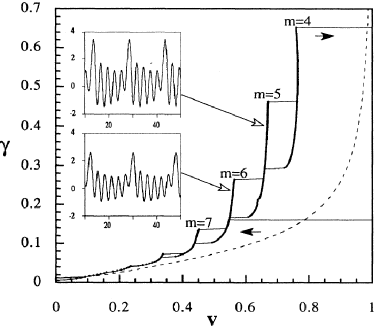
A relevant physical realization of the FK model is provided by an array of coupled long Josephson junctions (JJs) JJ1 ; JJ2 (each junction is a narrow dielectric layer separating two bulk superconductors Barone ). An accurate model of the array is provided by Eq. (24), where $f_{n}\equiv f$ represents the bias current applied to each junction, while $\alpha$ is the coefficient of Ohmic loss. Especially interesting is this version of the FK with periodic boundary conditions, which corresponds to the circular JJ array built of $N$ junctions Cirillo ; Strogatz , as it gives rise to resonant interaction between a kink (in terms of JJs, it is a fluxon, i.e., quantum of the magnetic flux), moving at velocity $c$ in the ring-shaped array, and phonon modes whose phase velocity $\chi/p$, determined by dispersion relation (25), may coincide with $c$. The periodicity of the array imposes the “quantization” condition on wavenumber $p$ in (25),

$$p=\left(2\pi/hN\right)m,\leavevmode\nobreak\ m=1,2,3,...\leavevmode\nobreak\ .$$ (31)

The analysis of the kink-phonon interaction leads to a dependence of the fluxon’s velocity $c$ on the driving force (current), $f$, in the form of resonant Shapiro steps Shapiro connected by hysteretic jumps, as shown in Fig. 1. This dependence predicts an experimentally observable current-voltage characteristic of the JJ system, as the voltage is proportional to $c$. The measured characteristic was found to be very close to the theoretical prediction Cirillo .

Figure 1: The predicted relation between the velocity of the discrete kink, travelling in the ring-shaped FK lattice composed of $N=10$ sites, subject to periodic boundary conditions, and the driving force. Numbers $m$, which label different vertical resonant steps, denote the “quantization” orders in Eq. (31). Arrows indicate directions of hysteretic jumps between the steps, and the dashed curve represents the $f(c)$ dependence in the continuum version of the system. Insets display dependences $\dot{u}_{n}$, which are proportional to the local voltage in the underlying JJ array, at the system’s midpoint, corresponding to two points in the $f(c)$ (current-voltage) characteristic marked by arrows. Parameters in Eq. (24) are $h=1$ and $\alpha=0.1$. Reproduced from Cirillo

Lastly, it is relevant to mention that the FK model also supports breathers, i.e. localized modes which are periodically oscillating functions of time Braun ; Aubry1 ; Floria ; Gendelman . In the continuum limit, the breathers naturally carry over into the well-known exact breather solutions of the sG equation (20),

III Nonlinear Schrödinger (NLS) lattices

III.1 One-dimensional (1D) solitons

III.1.1 Fundamental states

DNLS equation (3) gives rise to discrete solitons, which cannot be represented by analytical solutions, but can be easily found in a numerical form. General properties of the soliton families can be understood by means of the variational approximation (VA). Results for solitons in models of the DNLS type are well known, being broadly represented in the literature DNLS-book . Therefore, basic results for discrete NLS solitons are summarized here in a brief form.

Most studies addressed the 1D version of (3), i.e.

$$i\dot{\psi}_{n}=-(1/2)\left(\psi_{n+1}+\psi_{n-1}-2\psi_{n}\right)-\left|\psi_{n}\right|^{2}\psi_{n},$$ (32)

where the nonlinearity coefficient is fixed to be $g=-1$, which corresponds to the self-focusing sign of the onsite nonlinearity (recall that the sign of $g$ may be flipped by means of the staggering transformation (4)). The DNLS equation conserves two dynamical invariants, viz., the total norm,

$$N=\sum_{n=-\infty}^{+\infty}\left|\psi_{n}\right|^{2},$$ (33)

and Hamiltonian (energy),

$$H=\sum_{n=-\infty}^{+\infty}\left[(1/2)\left|\psi_{n}-\psi_{n-1}\right|^{2}-(1/4)\left|\psi_{n}\right|^{4}\right].$$ (34)

A fundamental property of the DNLS equation with the self-attractive onsite nonlinearity is the modulational instability of its spatially homogeneous state Peyrard .

Stationary solutions to (32) with real frequency $\omega$ are looked for as

$$\psi_{n}(t)=e^{-i\omega t}u_{n},$$ (35)

with real amplitudes $u_{n}$ satisfying the discrete equation,

$$\omega u_{n}=-(1/2)\left(u_{n+1}+u_{n-1}-2u_{n}\right)-u_{n}^{3}.$$ (36)

While (36) does not admit exact analytical solutions, the VA produces quite accurate approximations for discrete solitons. The VA is based on the Lagrangian, from which (36) can be derived by means of the variation with respect to discrete field $u_{n}$:

$$L=\sum_{n=-\infty}^{+\infty}\left\{(1/4)\left[\left(u_{n}-u_{n-1}\right)^{2}-u_{n}^{4}\right]-\omega u_{n}^{2}\right\}.$$ (37)

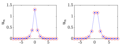
The use of the VA is based on a particular ansatz, i.e. a trial analytical expression which aims to approximate the solution Progress . The only discrete ansatz for which analytical calculations are feasible is represented by the exponential function Weinstein ; Papa ; Dave-VA ; Gorder . In particular, an onsite-centered (OC) discrete soliton, i.e. one with a single maximum (which is placed, by definition, at site $n=0$) is approximated by

$$\left(u_{n}\right)_{\mathrm{onsite}}=A\exp\left(-a|n|\right),$$ (38)

with $a>0$. The corresponding norm, calculated as per (33), is

$$N_{\mathrm{ansatz}}=A^{2}\coth a\text{.}$$

Note that ansatz (38) works well for strongly and moderately discrete solitons (see Fig. 2 below), but it is not appropriate for broad (quasi-continuum) modes, which are approximated by the commonly known soliton solution of the NLS equation (the 1D version of (1) with $U=0$),

$$\psi\left(x,t\right)=\eta\leavevmode\nobreak\ \mathrm{sech}\left(\eta\left(x-\xi\right)\right)\exp\left(i\eta^{2}t\right),$$ (39)

with a large width, $\eta^{-1}\gg 1$, and central coordinate $\xi$.

For intersite-centered (IC) discrete solitons, with two symmetric maxima placed at two adjacent sites of the lattice, $n=0$ and $n=1$ (and a formal central point located between the sites, hence the name of these modes), an appropriate ansatz is

$$\left(u_{n}\right)_{\mathrm{intersite}}=A\exp\left(-a|n-1/2|\right).$$ (40)

The substitution of ansatz (38) in Lagrangian (37) and straightforward calculations yield the following effective Lagrangian:

$$L_{\mathrm{eff}}=(A^{2}/2)\coth(a/2)-(A^{4}/4)\coth\left(2a\right)-\omega A^{2}\coth a.$$ (41)

Then, for given $\omega<0$ (the solitons with $\omega>0$ do not exist), the squared amplitude, $A^{2}$, and inverse width, $a$, of the discrete soliton are predicted by the Euler-Lagrange equations,

$$\frac{\partial L_{\mathrm{eff}}}{\partial\left(A^{2}\right)}=\frac{\partial L_{\mathrm{eff}}}{\partial a}=0.$$ (42)

This corresponding system of algebraic equations for $A^{2}$ and $a$ can be easily solved numerically. A similar analysis was performed for the IC solitons, starting with ansatz (40). The VA produces quite accurate predictions for solitons of both types, see Fig. 2 and Ref. Needs07 .

Figure 2: Comparison of a typical OC (left panel) and IC (right panel) 1D discrete solitons, obtained as numerical solutions of (36), shown by chains of blue dots, and their counterparts produced by the VA (shown by red open circles). In this figure, $\omega=-1$, see Eq. (35).

An extended version of VA for 1D discrete solitons was elaborated for nonstationary solutions, and compared to their numerically generated counterparts Weinstein ; Dave-VA . Moreover, it was demonstrated that VA may be applied, in a more sophisticated form, even to a challenging problem of collisions of moving discrete solitons Papa . Further considerations addressed false instabilities, which are sometimes predicted by the nonstationary VA Hadi-false instability , and rigorous justification of the VA rigorous . Finally, the VA and full numerical considerations demonstrate that the entire family of the OC discrete solitons is stable, while all the IC ones are unstable DNLS-book .

III.1.2 Mobility of 1D discrete solitons

The DNLS equation does not admit solutions for moving discrete solitons. Indeed, even in the quasi-continuum approximation, soliton (39) is running through the effective PN potential, which, for 1D DNLS modes, is

$$U_{\mathrm{PN}}(\xi)=-\frac{\pi^{4}}{3\sinh\left(\pi^{2}/\eta\right)}\cos\left(2\pi\xi\right),$$ (43)

cf. expression (30) for the PN barrier in the FK model. The periodic acceleration and deceleration of the quasi-continuous soliton moving across the PN potential gives rise to emission of small-amplitude “phonon” waves, i.e., losses which brake the motion. However, the emission effect is extremely weak in direct simulations of the DNLS equations, allowing the 1D discrete solitons to run indefinitely long Feddersen . On the other hand, discrete solitons in the 2D DNLS equation (see the following subsection) have no mobility. This is explained by the fact that the above-mentioned quasi-collapse effect Laedke makes them very narrow modes strongly pinned to the underlying lattice.

The mobility of 1D discrete solitons in NLS lattices may be essentially enhanced by means of the nonlinearity management technique management , i.e., replacing coefficient $g$ in the 1D version of (3) by a combination of constant (“dc”) and time-periodic (“ac”) terms JC1 :

$$i\dot{u}_{n}+u_{n+1}+u_{n-1}-2u_{n}+\left[g_{\mathrm{dc}}+g_{\mathrm{ac}}\sin(\omega t)\right]|u_{n}|^{2}u_{n}=0.$$ (44)

Similar to the situation for the damped driven TL, outlined above, discrete solitons may move across the lattice at special values of the velocity, determined by the resonance between the periodic passage of lattice sites by the soliton and periodically oscillating ac component of the nonlinearity coefficient in (44), cf. (19):

$$\left(c_{\mathrm{res}}\right)_{N}^{(M)}=\frac{M\omega}{2\pi N},$$ (45)

where integers $N$ and $M$ determine the order of the resonance. This prediction was corroborated by simulations of (44) JC1 .

III.1.3 Higher-order modes in the 1D DNLS equation: twisted solitons and bound states

In addition to the OC and IC solitons, which are fundamental states, Eq. (36) admits stable higher-order states in the form of twisted modes, which are subject to the antisymmetry condition, $u_{n}=-u_{1-n}$ twisted . Such states exist and are stable only in a strongly discrete form, vanishing in the continuum limit.

Stable discrete NLS solitons of the OC type may form bound states, which also represent higher-order modes of the DNLS equation. They are stable in the out-of-phase form, i.e., for opposite signs of the bound solitons bound states ; bound states 2 (the same is true for 2D discrete solitons Bishop ). Stationary bound states do not exist either in the continuum limit, where bound states of NLS solitons are represented solely by periodically oscillating breathers Satsuma Yajima .

III.2 Two-dimensional (2D) discrete solitons and solitary vortices in quiescent and rotating lattices

III.2.1 Static lattices

The 2D cubic DNLS equation is a straightforward extension of the 1D equation (32). In particular, its stationary form is

$$\omega u_{n}=-(1/2)\left(u_{m+1,n}+u_{m-1,n}+u_{m,n+1}+u_{m,n-1}-4u_{m,n}\right)-\left|u_{m,n}\right|^{2}u_{m,n},$$ (46)

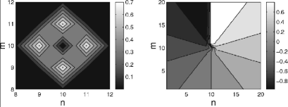
cf. (36), where the stationary discrete wave function, $u_{m,n}$, may be complex. Fundamental-soliton solutions to (46) can also be predicted by means of VA Weinstein-2D ; Chong (see (52) below for the simplest 2D ansatz). More interesting in the 2D case are discrete solitons with embedded vorticity, which were introduced in we (see also they ). Vorticity, alias topological charge, is defined as $\Delta\varphi/\left(2\pi\right)$, where $\Delta\varphi$ is a change of the phase of complex discrete wave function $u_{m,n}$, corresponding to any contour surrounding the vortex’ pivot. Stability is an important issue for 2D discrete solitons, because it is commonly known that, in the continuum limit, the NLS equation in 2D gives rise solely to unstable solitons, including fundamental ones (usually called Townes’ solitons Townes ), which are unstable against the critical collapse Gadi , and solitons with embedded vorticity Minsk , which are still more unstable PhysD .

A typical example of a stable 2D discrete soliton is displayed in Fig. 3. 2D fundamental and vortex solitons, with topological charges $S=0$ and $1$, remain stable at $-\omega>|\omega_{\mathrm{cr}}^{(S=0)}|\approx 0.50$  and $-\omega>|\omega_{\mathrm{cr}}^{(S=1)}|\approx 1.23$, respectively we , while the higher-order localized discrete vortices with $S=2$ and $4$ are unstable, being replaced by stable modes in the form of quadrupoles and octupoles Zhigang . Higher-order vortex solitons with $S=3$ are stable only in a strongly discrete form, at $-\omega>|\omega_{\mathrm{cr}}^{(S=2)}|\approx 4.94$.

Figure 3: A stable discrete vortex soliton with topological charge $S=1$, produced by Eq. (46). The left and right panels show, respectively, distributions of the absolute value and phase of complex wave function $u_{m,n}$ in the plane of $\left(m,n\right)$.

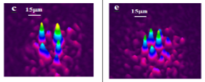
The theoretically predicted 2D discrete solitons with vorticity $S=1$ were experimentally created in Kivshar and Segev , using a photorefractive crystal. Unlike uniform media of this type, where delocalized (“dark”) optical vortices were originally produced Zhig1 ; Zhig2 , these works made use of a deep virtual photonic lattice as a quasi-discrete medium supporting nonlinear optical modes in light beams with extraordinary polarization (while the photonic lattice was induced by the interference of quasi-linear beams in the ordinary polarization). Intensity distributions observed in vortex solitons of the OC and IC types are displayed in Fig. 4.

Figure 4: Quasi-discrete optical solitons with vorticity $S=1$, created in a bulk photorefractive crystal with an induced deep photonic lattice. The left and right panels display, respectively, OC and IC vortex solitons. Reproduced from Segev .

Another interesting result demonstrated (and theoretically explained) in deep virtual photonic lattices is a possibility of periodic flipping of the topological charge of a vortex soliton initially created with $S=2$ Chen .

III.2.2 Rotating lattices

Dynamics of BEC loaded in OLs rotating at angular velocity $\Omega$, as well as the propagation of light in a twisted nonlinear photonic crystal with pitch $\Omega$, is modeled by the 2D version of Eq. (1), written in the rotating reference frame:

$$i\psi_{t}=-\left((1/2)\nabla^{2}+\Omega\hat{L}_{z}\right)\psi-\varepsilon\left[\cos\left(kx\right)+\cos(ky)\right]\psi+g|\psi|^{2}\psi,$$ (47)

where $\hat{L}_{z}=i(x\partial_{y}-y\partial_{x})\equiv i\partial_{\theta}$ is the operator of the $z$-component of the orbital momentum ($\theta$ is the angular coordinate in the $\left(x,y\right)$ plane). In the tight-binding approximation, Eq. (47) is replaced by the following variant of the DNLS equation JC2 :

$$i\dot{\psi}_{m,n}=-(C/2)\left\{\left(\psi_{m+1,n}+\psi_{m-1,n}+\psi_{m,n+1}+\psi_{m,n-1}-4\psi_{m,n}\right)\right.$$

$$\left.-i\Omega\left[m\left(\psi_{m,n+1}-\psi_{m,n-1}\right)-n\left(\psi_{m+1,n}-\psi_{m-1,n}\right)\right]\right\}+g|\psi_{m,n}|^{2}\psi_{m,n}\leavevmode\nobreak\ ,$$ (48)

where $C$ is the intersite coupling constant. In JC2 , stationary solutions to (48) were looked for in the form of ansatz (35), fixing $\omega\equiv-1$ and varying $C$ in (48) as a control parameter. Two species of localized states were thus constructed: off-axis fundamental discrete solitons, placed at distance $R$ from the rotation pivot, and on-axis ($R=0$) vortex solitons, with vorticities $S=1$ and $2$. At a fixed value of rotation frequency $\Omega$, a stability interval for the fundamental soliton, $0<C<C_{\max}^{\mathrm{(fund)}}(R)$, monotonously shrinks with the increase of $R$, i.e., most stable are the discrete solitons with the center placed at the rotation pivot. Vortices with $S=1$ are gradually destabilized with the increase of $\Omega$ (i.e., their stability interval, $0<C<C_{\max}^{\mathrm{(vort)}}(\Omega)$, shrinks). On the contrary, a remarkable finding is that vortex solitons with $S=2$, which, as said above, are completely unstable in the usual DNLS equation with $\Omega=0$, are stabilized by the rotation, in an interval $0<C<C_{\mathrm{cr}}^{(S=2)}(\Omega)$, with $C_{\mathrm{cr}}^{(S=2)}(\Omega)$ growing as a function of $\Omega$. In particular, $C_{\mathrm{cr}}^{(S=2)}(\Omega)\approx 2.5\Omega$ at small $\Omega$ JC2 .

III.3 Spontaneous symmetry breaking in linearly-coupled lattices

A characteristic feature of many nonlinear dual-core systems, built of two identical linearly-coupled waveguides with intrinsic nonlinearity, is a spontaneous-symmetry-breaking (SSB) bifurcation, which destabilizes the symmetric ground state, with equal components in the coupled cores, and creates stable asymmetric ones, when the nonlinearity strength exceeds a critical value SSB . A system of linearly-coupled DNLS equations is a basic model for SSB in discrete settings. Its 2D form is herring

$$i\dot{\phi}_{n} = -(1/4)\left(\phi_{m+1,n}+\phi_{m-1,n}+\phi_{m,n+1}+\phi_{m,n-1}-4\phi_{m,n}\right)-\left|\phi_{m,n}\right|^{2}\phi_{m,n}-K\psi_{m,n}\leavevmode\nobreak\ ,$$

$$i\dot{\psi}_{n} = -(1/4)\left(\psi_{m+1,n}+\psi_{m-1,n}+\psi_{m,n+1}+\psi_{m,n-1}-4\psi_{m,n}\right)-\left|\psi_{m,n}\right|^{2}\psi_{m,n}-K\phi_{m,n}\leavevmode\nobreak\ ,$$ (49)

where $\phi_{m,n}$ and $\psi_{m,n}$ are discrete fields, and $K>0$ accounts for the linear coupling between them. Stationary states are looked for as $\left(\phi_{m,n},\psi_{m,n}\right)=\exp\left(-i\omega t\right)\left(u_{m,n},v_{m.n}\right)$, where the linear coupling makes it necessary to have identical frequencies, $\omega$, in both components. Real stationary fields are characterized by their norms,

$$E_{u,v}=\sum_{m,n=-\infty}^{+\infty}\left(u_{m,n}^{2},v_{m,n}^{2}\right),$$ (50)

which define the asymmetry degree of the symmetry-broken states:

$$r=\left(E_{u}-E_{v}\right)/\left(E_{u}+E_{v}\right).$$ (51)

The present system can be analyzed by means of the VA, which is based on the simplest ansatz (cf. its 1D counterpart (38)):

$$\left(u_{m,n},v_{m,n}\right)=\left(A,B\right)\exp\left[-a\left(|m|+|n|\right)\right],$$ (52)

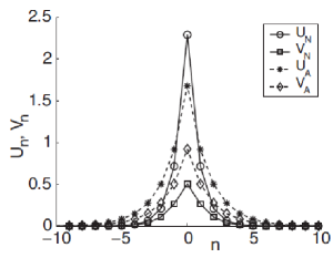
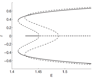
with inverse width $a$ and amplitudes, $A$ and $B$, of the two components. The ansatz accounts for the SSB in the case of $A\neq B$. A typical example of a stable 2D discrete OC soliton is displayed in Fig. 5a, which corroborates accuracy of the VA. The full set of symmetric and asymmetric 2D discrete solitons is characterized, in Fig. 5b, by the dependence of asymmetry parameter $r$, defined in (51), on the total norm, $E\equiv E_{u}+E_{v}$. It is seen that the SSB bifurcation is one of a clearly subcritical type Iooss , with the two branches of broken-symmetry states originally going backward as unstable ones, and getting stable after passing the turning point. Accordingly, Fig. 5b demonstrates a considerable bistability area, where symmetric and asymmetric states coexist as ones stable against small perturbations.

Figure 5: (a) A stable 2D two-component discrete soliton with spontaneously broken symmetry between the components, generated by system (49). The 2D soliton, with total norm $E\equiv E_{u}+E_{v}=1.435$, is displayed by means of its 1D cross section. Symbols labelled $\left(U_{\mathrm{N}},V_{\mathrm{N}}\right)$ and $\left(U_{\mathrm{A}},V_{\mathrm{A}}\right)$ stand, respectively, for the components of the numerically constructed soliton and its analytical counterpart predicted by the VA based on ansatz (52). (b) Families of 2D discrete solitons of the OC type, generated by system (49), are shown by means of curves $r(E)$ (where $r$ is the asymmetry parameter (51)). The dashed-dotted curve shows the VA prediction, while the solid and dashed ones depict stable and unstable solitons produced by the numerical solution. Reproduced from herring .

IV Ablowitz-Ladik and Salerno-model lattices

IV.1 1D models

1D models of AL and SM types, which are defined by Eqs. (5) and (6), conserve the total norm, but its definition is different from the straightforward one, given by Eq. (33) for the DNLS equation; namely,

$$N_{\mathrm{AL,SM}}=(1/\mu)\sum_{n}\ln\left|1+\mu|\psi_{n}|^{2}\right|$$ (53)

AL ; Cai . The Hamiltonian of the AL and SM equations is also essentially different from the “naive” DNLS Hamiltonian given by Eq. (34). As found in the original work of Ablowitz and Ladik, the Hamiltonian of their model is

$$H_{\mathrm{AL}}=-\sum_{n}\left(\psi_{n}\psi_{n+1}^{\ast}+\psi_{n+1}\psi_{n}^{\ast}\right),$$ (54)

while for the SM, it is Cai

$$H_{\mathrm{SM}}=-\sum_{n}\left[\left(\psi_{n}\psi_{n+1}^{\ast}+\psi_{n+1}\psi_{n}^{\ast}\right)+(2/\mu)|\psi_{n}|^{2}\right]+(2/\mu)N_{\mathrm{AL}}.$$ (55)

The price paid for ostensible “simplicity” of expression (54) is the complex form of the respective Poisson brackets, which determine the dynamical equations in terms of the Hamiltonian as $d\psi_{n}/dt=\left\{H,\psi_{n}\right\}$. For the AL and SM models, the Poisson brackets, written for a pair of arbitrary functions of the discrete field variables, $B\left(\psi_{n},\psi_{n}^{\ast}\right),$ $C\left(\psi_{n},\psi_{n}^{\ast}\right)$, are

$$\left\{B,C\right\}=i\sum_{n}\left(\frac{\partial B}{\partial\psi_{n}}\frac{\partial C}{\partial\psi_{n}^{\ast}}-\frac{\partial B}{\partial\psi_{n}^{\ast}}\frac{\partial C}{\partial\psi_{n}}\right)\left(1+\mu\left|\psi_{n}\right|^{2}\right).$$ (56)

As mentioned above, the continuum limit of the SM is represented by Eq. (8) Zaragoza . This continuous equation conserves the total norm and Hamiltonian, written in terms of variables $\Psi\left(x\right)$ (see Eq. (7)), which are straightforward continuum counterparts of expressions (53)-(55):

$$\left(N_{\mathrm{AL}}\right)_{\mathrm{cont}} = \frac{1}{\mu}\int_{-\infty}^{+\infty}dx\leavevmode\nobreak\ {\ln}\left|1+\mu|\Psi|^{2}\right|,$$ (57)

$$\left(H_{\mathrm{SM}}\right)_{\mathrm{cont}} = \int_{-\infty}^{+\infty}dx\left[\left|\Psi_{x}\right|^{2}-2\left(\frac{1}{\mu}+1\right)|\Psi|^{2}\right]+\frac{2}{\mu}\left(N_{\mathrm{AL}}\right)_{\mathrm{cont}}$$ (58)

IV.2 Discrete 1D solitons

The AL equation (5) gives rise to an exact solution for solitons in the case of self-focusing nonlinearity, $\mu>0$. Setting $\mu\equiv+1$ by means of rescaling, the solution is

$$\psi_{n}(t)=\left(\sinh\beta\right)\mathrm{sech}\left[\beta(n-\xi(t))\right]\exp\left[i\alpha\left(n-\xi(t)\right)-i\varphi(t)\right],$$ (59)

where $\beta$ and $\alpha$ are arbitrary real parameters that determine the soliton’s amplitude, $A\equiv\sinh\beta$, its velocity, $V\equiv\dot{\xi}=2\beta^{-1}\left(\sinh\beta\right)\sin\alpha$, and overall frequency $\Omega\equiv\dot{\varphi}=-2\left[\left(\cosh\beta\right)\cos\alpha+(\alpha/\beta)\left(\sinh\beta\right)\sin\alpha\right]$.

The existence of exact solutions for traveling solitons in the discrete system is a highly nontrivial property of the AL equation, which follows from its integrability. If the system is not integrable, motion of a discrete soliton through a lattice is hampered by emission of radiation, even if this effect may seem very weak in direct simulations Feddersen . On the other hand, there are some special discrete equations which are not integrable, but admit particular solutions for traveling solitons (at exceptional values of the velocity, rather than at an arbitrary velocities, as in the case of the AL solitons Kevrekidis ; Oxtoby .

The stationary version of the SM, obtained by the substitution of the usual ansatz (35), with real $u_{n}$, in (6), is

$$\omega u_{n}=-\left(u_{n+1}+u_{n-1}\right)\left(1+\mu u_{n}^{2}\right)-2u_{n}^{3},$$ (60)

cf. (36). Discrete solitons in the nonintegrable SM equation (6) with $\mu>0$, i.e. with noncompeting intersite and onsite self-focusing nonlinearities, were investigated by means of numerical methods Cai ; Cai97 ; Dmitriev03 . It has been demonstrated that the SM gives rise to static (and, sometimes, approximately mobile Cai97 ) solitons at all positive values of $\mu$.

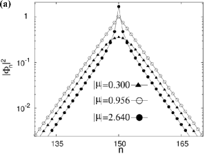
Another possibility is to consider the SM with $\mu<0$, which features competing nonlinearities, as the intersite cubic term, with coefficient $\mu<0$ in (6), which accounts for nonlinear coupling between adjacent sites of the lattice, and the onsite term in (6) (the last term in that equation) represent, respectively, self-defocusing and focusing nonlinear interactions. It was found Zaragoza that this version of the SM gives rise to families of quiescent discrete solitons, which are looked for in the usual form (35), with $\omega<0$ and real amplitudes $u_{n}$, of two different types. One family represents ordinary discrete solitons, similar to those generated by the DNLS equation. Another family represents cuspons, featuring higher curvature of their profile at the center than exponential shapes. Examples of numerically found stable discrete solitons of these types are displayed in Fig. 6a. The border between the ordinary discrete solitons and cuspons is represented by a special discrete mode, in the form of a stable peakon, which is also shown in Fig. 6a.

The continuum limit of the SM with competing nonlinearities, given by (8) with $\mu<0$, produces continuous solitons in the usual form, $\Psi=\exp\left(-i\omega t\right)U(x)$, in the frequency band $0<-\omega<1/|\mu|-1$, provided that $|\mu|<1$. At the edge of the soliton band, i.e. at $\omega=-\left(1/|\mu|-1\right)$, (8) gives rise to an exact solution in the form of the continuous peakon $U_{\mathrm{peakon}}(x)=\left(1/\sqrt{|\mu|}\right)\exp\left(-\sqrt{\left(1/|\mu|\right)-1}|x|\right)$Zaragoza . For continuous solutions, the name of “peakon” implies a jump of the derivative at the central point, while cuspons do not exist in the continuum limit.

Figure 6: (a) Examples of three different types of discrete solitons, shown on the logarithmic scale, which are produced by Eq. (60), i.e., the Salerno model, with competing nonlinearities ($\mu<0$), at $\omega=-2.091$: an ordinary soliton for $\mu=-0.3$, a peakon for $\mu=-0.956$, and a cuspon for $\mu=-2.64$. In the figure, $\left|\Phi_{n}\right|$ has the same meaning as $u_{n}$ in Eq. (60). (b) The norm of the discrete solitons in the Salerno model with competing nonlinearities vs. the frequency (denoted here $\omega_{b}$, instead of $\omega$), for $\mu=-0.884$. Reproduced from Zaragoza .

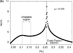The stability analysis of discrete solitons produced by the SM with competing nonlinearities demonstrate that only a small subfamily of ordinary solitons is unstable, while all cuspons, including the peakon, are stable. For fixed $\mu=-0.884$, a typical situation for families of discrete solitons in the SM with competing nonlinearities is presented in Fig. 6b, which shows norm (53) as a function of $|\omega|$. The plot clearly demonstrates that ordinary solitons and cuspons are separated by the peakon, as mentioned above. Except for the part of the ordinary-soliton family with the negative slope, $d{N}/d(|\omega|)<0$, which is marked in Fig. 6b, the discrete solitons are stable. In particular, it is worthy to note that the cuspons and peakon are completely stable modes. The instability of the segment of the family of ordinary discrete solitons with $d{N}/d(|\omega|)<0$ exactly agrees with the prediction of the well-known Vakhitov-Kolokolov criterion Vakh . On the other hand, it is seen from Fig. 6b that the VK criterion, being valid for the ordinary solitons, is actually reversed for the cuspons Zaragoza .

As mentioned above, antisymmetric bound states of DNLS solitons are stable, while symmetric bound states are unstable bound states ; bound states 2 . As shown in Zaragoza , the same is true for bound states of ordinary discrete solitons in the SM. However, a noteworthy finding is that, in the framework of the SM with competing nonlinearities, the situation is exactly opposite for the cuspons: their symmetric and antisymmetric bound states are stable and unstable, respectively Zaragoza .

IV.3 The two-dimensional Salerno model and its discrete solitons

The 2D version of the SM was introduced in Zaragoza2D . It is based on the following equation, cf. (6),

$$i\dot{\psi}_{n,m} = -\left[\left(\psi_{n+1,m}+\psi_{n-1,m}\right)+C\left(\psi_{n,m+1}+\psi_{n,m-1}\right)\right]$$ (61)

$$\times \left(1+\mu\left|\psi_{n,m}\right|^{2}\right)-2\left|\psi_{n,m}\right|^{2}\psi_{n,m}\;,$$

where real constant $C>0$ accounts for a possible anisotropy of the 2D lattice. Similar to its 1D version, Eq. (61) conserves the norm and Hamiltonian, cf. (53) and (55),

$$\left(N_{\mathrm{AL}}\right)_{\mathrm{2D}}=(1/\mu)\sum_{m,n}\ln\left|1+\mu|\psi_{n,m}|^{2}\right|\;,$$ (62)

$$\left(H_{\mathrm{AL}}\right)_{\mathrm{2D}}=-\sum_{n,m}\left[\left(\psi_{n,m}\psi_{n+1,m}^{\ast}+\psi_{n+1,m}\psi_{n,m}^{\ast}\right)+C\left(\psi_{n,m}\psi_{n,m+1}^{\ast}+\psi_{n,m+1}\psi_{n,m}^{\ast}\right)\right.$$

$$\left.+(2/\mu)|\psi_{n,m}|^{2}\right]+(2/\mu)\left(N_{\mathrm{AL}}\right)_{\mathrm{2D}}.\;$$ (63)

The continuum limit of this model is a 2D continuous equation which is a straightforward extension of its 1D counterpart (8):

$$i\Psi_{t}+\left(1+\mu\left|\Psi\right|^{2}\right)\left(\Psi_{xx}+\Psi_{yy}\right)+2\left[(1+C)\mu+1\right]|\Psi|^{2}\Psi=0.$$ (64)

Note that term in $\mu\left|\Psi\right|^{2}\left(\Psi_{xx}+\Psi_{yy}\right)$ prevents the onset of the collapse in Eq. (64).

2D solitons are looked for in the same form as their 1D counterparts, $\psi_{mn}(t)=e^{-i\omega t}u_{mn}$, cf. (35). In the most interesting case of the competing nonlinearities, $\mu<0$, the situation is similar to that outlined above for SM in 1D: there are ordinary discrete solitons, which have their stability and instability regions, and 2D cuspons, which are entirely stable in their existence region. Typical 2D solitons of both types are displayed in Fig. 7. Also similar to the 1D case, ordinary solitons and cuspons are separated by 2D peakons, which are stable. In addition to that, antisymmetric bound states of ordinary 2D discrete solitons, and symmetric complexes built of 2D cuspons, are stable, while the bound states with opposite parities are unstable, also like in the 1D model.

Figure 7: Discrete solitons in the isotropic ($C=1$) 2D Salerno model with competing nonlinearities [$\mu<0$ in (61)], obtained for frequency $\omega=-4.22$: (a) a regular soliton at $\mu=-0.2$; (b) a cuspon at $\mu=-0.88$. Reproduced from Zaragoza2D .

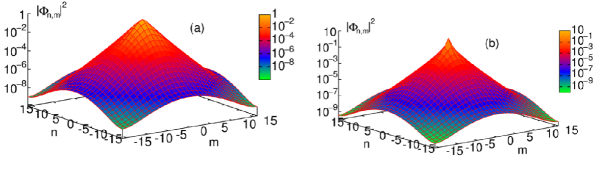
Along with the fundamental solitons, the 2D SM with the competing nonlinearities gives rise to vortex-soliton modes with narrow stability regions Zaragoza2D . In the 2D SM with non-competing nonlinearities, unstable vortex solitons spontaneously transform into fundamental solitons, losing their vorticity (this is possible because the angular momentum is not conserved in the lattice system). The situation is essentially different in the 2D SM with competing nonlinearities, where unstable vortex modes transform into vortical breathers, i.e., persistently oscillating localized modes that keep the original vorticity.

V A brief survey of semi-discrete systems

A topic which may be a subject for a separate review, is semi-discrete systems, i.e., 2D settings which are discrete in one direction and continuous in the other. Accordingly, such systems can create semi-discrete solitons. A system of this type which was explored in detail is an array of optical fibers Rubenchik , modeled by a system of coupled NLS equations for amplitudes $u_{n}\left(z,\tau\right)$ of electromagnetic waves in individual fibers:

$$i\partial_{z}u_{n}+(1/2)D\partial_{\tau}^{2}u_{n}+(\kappa/2)\left(u_{n+1}+u_{n-1}-2u_{n}\right)+\left|u_{n}\right|^{2}u_{n}=0,$$ (65)

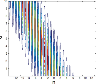
where $D$ is the group-velocity-dispersion coefficient in each fiber, and $\kappa>0$ is the coefficient of coupling between adjacent fibers in the array. It supports semi-discrete solitons in the case of anomalous dispersion, i.e. $D>0$. A remarkable property of semi-discrete modes generated by Eq. (65) is their ability to stably move across the array, under the action of a kick applied to them at $z=0$ Blit :

$$u_{n}(\tau)\rightarrow\exp\left(ian\right)u_{n}(\tau),$$ (66)

with real $a$. An example of such a moving mode is displayed in Fig. 8. This property may be compared to the above-mentioned mobility of 1D discrete solitons in the DNLS equation Feddersen .

Figure 8: An example of a semi-discrete spatiotemporal mode, generated by Eq. (65), which performs stable transverse motion under the action of the kick, defined according to (66), with $a=1.5$. The cross section of the plot at any fixed $z$ shows the distribution of power $\left|u_{n}(\tau)\right|^{2}$ for each $n$. Reproduced from Blit .

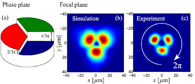
Similarly, quasi-discrete settings modeled by an extension of (65) with two transverse spatial coordinates were used for the creation for spatiotemporal optical solitons (“light bullets”) Jena , as well as soliton-like transient modes with embedded vorticity Jena-vort . Waveguides employed in those experiments feature a transverse hexagonal-lattice structure, written in bulk silica by means of an optical technology. A spatiotemporal vortex state (in the experiment, it is actually a transient one) in the bundle-like structure is presented by Fig. 9, which displays both numerically predicted and experimentally observed distributions of intensity of light in the transverse plane, together with a phase plate used in the experiment to embed the vorticity into the incident spatiotemporal pulse which was used to create the mode.

Figure 9: A semi-discrete vortex soliton in a hexagonal quasi-discrete array of waveguides made in bulk silica. (a) A phase plate used for imprinting the vortex structure into the input beam. (b,c) Numerically simulated and experimentally observed (transient) intensity distributions in the transverse plane, with phase shifts $2\pi/3$ between adjacent peaks. Reproduced from Jena-vort . Creative Commons Attribution License (CC BY) http://creativecommons.org/licenses/by/3.0/.

A new type of semi-discrete solitons was recently reported in Raymond , in the framework of an array of linearly coupled 1D GPEs, including the Lee-Hung-Yang correction, which represents an effect of quantum fluctuations around the mean-field states of a binary BEC Petrov1 ; Petrov2 . The system is

$$i\partial_{t}\psi_{j}=-{(1/2)}\partial_{zz}\psi_{j}-\left(1/2\right)\left(\psi_{j+1}-2\psi_{j}+\psi_{j-1}\right)+g|\psi_{j}|^{2}\psi_{j}-|\psi_{j}|\psi_{j},$$ (67)

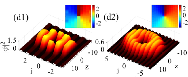
where $\psi_{j}(z)$ is the mean-field wave function in the $j$-th core, the self-attractive quadratic term represents the Lee-Hung-Yang effect, and $g>0$ accounts for the mean-field self-repulsion. This system gives rise to many families of semi-discrete solitons, including a novel species of semi-discrete vortex solitons. Typical examples of such stable states are displayed in Fig. 10.

Figure 10: Left and right panels display, respectively, examples of amplitude and phase profiles of stable OC and IC semi-discrete vortex solitons produced by Eq. (67). Reproduced from Raymond .

Semi-discreteness of another type is possible in two-component systems, where one component is governed by a discrete equation, while the other one obeys a continuous equation. This type of two-component systems was introduced in Panoiu , addressing a second-harmonic-generating model, assuming that the continuous second-harmonic wave propagates in a slab with a continuous transverse coordinate, while the fundamental-harmonic field is concentrated in a discrete waveguiding array attached to the slab. Semi-discrete solitons of an inverted type, with the continuous fundamental-frequency component and discrete second harmonic one, were also constructed in Panoiu .

VI Conclusion

VI.1 Summary of the Chapter

The interplay of discreteness and intrinsic nonlinearity in various physical media gives rise to a great variety of static and dynamical states. Among them, especially interesting are self-trapped ones in the form of discrete solitons. The present Chapter aims to briefly review basic theoretical models combining discreteness and nonlinearity, and basic results for discrete solitons produced by such models. Essential experimental findings are included too (in particular, those for 2D and 3D discrete solitons with embedded vorticity). In many cases, discreteness helps to produce states which either do not exist or are unstable in continuum counterparts of discrete settings. In particular, the 1D DNLS equation gives rise to stable bound states of fundamental solitons, and the 2D DNLS equation readily creates fundamental and vortex solitons, whose counterparts are completely unstable in the continuum. On the other hand, some properties which are obvious in the continuum limit, such as mobility of solitons, are problematic in discrete settings.

The work in this area is currently in progress, and new results may be expected. A promising direction is to generate discrete counterparts of complex continuous modes with intrinsic topological structures. Some results obtained in this direction have already been reported, such as discrete solitons in a system with spin-orbit coupling Sandra , sophisticated 3D discrete modes with embedded vorticity 3Dvort ; 3Dvort2 , and discrete skyrmions skyrmion . A challenging task is experimental realization of such results which, thus far, were only predicted in the theoretical form.

VI.2 Topics not included in the Chapter

Due to length limitations, some essential models and methods are not considered here. One of them is the anti-continuum limit, which makes it possible to obtain “stems” for many families of discrete solitons by considering, at first, lattice models with no coupling between the sites. Using this approach, one can construct a great deal of modes, by formally putting together various solutions supported by non-interacting sites of the lattice. Then, the analysis allows one to identify solution branches that can be extended to small nonzero values of the intersite coupling. This method is efficient in constructing many families of discrete solitons in diverse models Aubry1 ; bound states 2 ; they ; Aubry2 .

Interaction of discrete solitons with local defects in the underlying lattice, as well as with interfaces and edges (surfaces, if the underlying lattice is two- or three-dimensional) is another vast area of theoretical and experimental studies. In particular, defects and surfaces may often help to create and stabilize localized modes which do not exist or are unstable in uniform lattices, such as Tamm Tamm and topological-insulator top-ins ; top-ins2 states.

Large topics are solitons in discrete dissipative nonlinear systems, and in systems subject to the condition of the parity-time ($\mathcal{PT}$) symmetry. In this Chapter, dissipative systems, which include friction and driving forces, are considered only in terms of TL and FK models (in particular, for arrays of Josephson junctions, in Fig. 1). Other dissipative versions of TL models are known too, in the form of LC transmission lines for electric pulses. They support traveling discrete solitons, which have been produced in theoretical and experimental forms LC1 ; LC2 ; LC3 .

In other contexts, basic nonlinear dissipative models are represented by discrete complex Ginzburg-Landau equations, i.e., DNLS equations with complex coefficients in front of onsite linear and nonlinear terms, which account for dissipative losses and compensating gain Hakim . These models give rise to discrete solitons which do not exist in continuous families, unlike the DNLS solitons, but rather as isolated attractors Efremidis1 ; Akhmed ; Efremidis2 .

Systems with $\mathcal{PT}$ symmetry are dissipative models which share many properties with conservative ones. They include mutually symmetric spatially separated linear gain and loss elements Bender ; Christod ; Christod2 . This arrangement makes it natural to consider $\mathcal{PT}$-symmetric systems with a discrete structure. Their experimental realization in optics Christod2 suggests to include the Kerr nonlinearity, thus opening the way to prediction of $\mathcal{PT}$-symmetric discrete solitons PTrev1 ; PTrev2 . In particular, various species of stable 1D and 2D discrete solitons were predicted in chains of $\mathcal{PT}$-symmetric elements PTsol1 ; PTsol0 ; PTsol2 ; PTsol3 ; PTsol4 ; PTsol5 . An example of $\mathcal{PT}$-symmetric solitons has been created experimentally in a similar discrete setting PTsol-observation .

References

- (1) C. Pethick, H. Smith, Bose-Einstein condensation in dilute gases (Cambridge University Press, Cambridge, 2002)
- (2) G. Fibich, The Nonlinear Schrödinger Equation: Singular Solutions and Optical Collapse (Springer, Heidelberg, 2015)
- (3) Yu.S. Kivshar, G. P. Agrawal, Optical Solitons: From Fibers to Photonic Crystals (Academic Press, San Diego, 2003)
- (4) O. Morsch, M. Oberthaler, Rev. Mod. Phys. 78, 179 (2006)
- (5) M.A. Porter, R. Carretero-González, P.G. Kevrekidis, B.A. Malomed, Chaos 15, 015115 (2005)
- (6) M. Skorobogatiy, J. Yang,Fundamentals of Photonic Crystal Guiding (Cambridge University Press, Cambridge, 2008)
- (7) D. N. Christodoulides, R. I. Joseph, Opt. Lett. 13, 794 (1988)
- (8) H.S. Eisenberg, Y. Silberberg, R. Morandotti, A.R. Boyd, J.S. Aitchison, Phys. Rev. Lett. 81, 3383 (1998)
- (9) D.N. Christodoulides, F. Lederer, Y. Silberberg, Nature 424, 817 (2003)
- (10) F. Lederer , G. I. Stegeman, D. N. Christodoulides, G. Assanto, M. Segev, Y. Silberberg, Phys. Rep. 463, 1 (2008)
- (11) F. Ye, D. Mihalache, B. Hu, N.C. Panoiu, Phys. Rev. Lett. 104, 106802 (2010)
- (12) A. Smerzi, A. Trombettoni, Phys. Rev. A 68, 023613 (2003)
- (13) A. Szameit, R. Keil, F. Dreisow, M. Heinrich, T. Pertsch, S. Nolte, A. Tünnermann, Opt. Lett. 34, 2838 (2009)
- (14) C. Chong, R. Carretero-González, B. A. Malomed, P.G. Kevrekidis, Physica D 240, 1205 (2011)
- (15) A. Szameit, T. Pertsch, S. Nolte, A. Tünnermann, F. Lederer, Phys. Rev. A 77, 043804 (2008)
- (16) E.W. Laedke, K. H. Spatschek, S.K. Turitsyn, Phys. Rev. Lett. 73, 1055 (1994)
- (17) P.G. Kevrekidis, The Discrete Nonlinear Schrödinger Equation: Mathematical Analysis, Numerical Computations, and Physical Perspectives (Springer, Berlin Heidelberg, 2009)
- (18) A. Locatelli, D. Modotto, D. Paloschi, C. De Angelis, Opt. Commun. 237, 97 (2004)
- (19) G. Herring, P. G. Kevrekidis, B. A. Malomed, R. Carretero-González, D. J. Frantzeskakis, Phys. Rev. E 76, 066606 (2007)
- (20) V.E. Zakharov, S.V. Manakov, S.P. Novikov, L.P. Pitaevskii, Solitons: The Inverse Scattering Method (Nauka Publishers, Moscow, 1980) [English translation: Consultants Bureau, New York, 1984]
- (21) M.J. Ablowitz, H. Segur, Solitons and Inverse Scattering Method (SIAM, Philadelphia, 1981)
- (22) F. Calogero, A. Degasperis, Spectral Transform and Solitons: Tools to Solve and Investigate Nonlinear Evolution Equations (North-Holland, New York, 1982)
- (23) A.C. Newell, Solitons in Mathematics and Physics (SIAM: Philadelphia, 1985)
- (24) M.J. Ablowitz, B. M. Herbst, SIAM J. Appl. Math. 50, 339 (1990)
- (25) D. Levi, M. Petrera, C. Scimiterna, Europhys. Lett. 84, 10003 (2008)
- (26) M.J. Ablowitz, J.F. Ladik, J. Math. Phys. 17, 1011 (1976)
- (27) M. Salerno, Phys. Lett. A 162, 381-384 (1992)
- (28) O. Dutta, A. Eckardt, P. Hauke, B. Malomed, M. Lewenstein, New J. Phys. 13, 023019 (2011)
- (29) O. Dutta, M. Gajda, P. Hauke, M. Lewenstein, D.-S. Luhmann, B.A. Malomed, T. Sowinski, J. Zakrzewski, Rep. Prog. Phys. 78, 066001 (2015)
- (30) J. Gómez-Gardeñes, B.A. Malomed, L.M. Floría, A.R. Bishop, Phys. Rev. E 73, 036608 (2006)
- (31) M. Toda, J. Phys. Soc. Jpn. 22, 431 (1967)
- (32) R.S. Johnson, A modern introduction to the mathematical theory of water waves (Cambridge University Press, Cambridge, 1997)
- (33) E. Fermi, J. Pasta, S. Ulam, Los Alamos Report LA-1940, p. 975 (1955)
- (34) G. Gallavoti (ed.), The Fermi-Pasta-Ulam Problem: A Status Report (Springer, Berlin Heidelberg, 2008)
- (35) M.A. Porter, N.J. Zabusky, B. Hu, D. K. Campbell, Am. Sci. 97, 214 (2009)
- (36) T. Dauxois, Phys. Today 6, 55 (2008)
- (37) N.J. Zabusky, M. D. Kruskal, Phys. Rev. Lett. 15, 240 (1965)
- (38) Ya.I. Frenkel, T. Kontorova, J. Phys. 1, 137 (1939)
- (39) Yu.S. Kivshar, O. M. Braun, The Frenkel-Kontorova Model: Concepts, Methods and Applications (Springer, Berlin Heidelberg, 2004)
- (40) B.A. Malomed, Phys. Rev. A 45, 4097 (1992)
- (41) T. Kuusela, J. Hietarinta, B. A. Malomed J. Phys. A 26, L21 (1993)
- (42) K.Ø. Rasmussen, B.A. Malomed, A. R. Bishop, N. Grønbech-Jensen, Phys. Rev. E 58, 6695-6699 (1998)
- (43) K.L. Johnson, Contact Mechanics (Cambridge University Press, Cambridge, 1985)
- (44) N. Boechler, G. Theocharis, S. Job, P.G. Kevrekidis, M.A. Porter, C. Daraio, Phys. Rev. Lett. 104, 244302 (2010)
- (45) O. Derzhko, J. Richter, M. Maksymenko, Int. J. Mod. Phys. B 29, 1530007 (2015)
- (46) D. Leykam, A. Andreanov, S. Flach, Adv. Phys. X 3, 1 (2018)
- (47) K. Zegadlo, N. Dror, N.V. Hung, M. Trippenbach, B. A. Malomed, Phys. Rev. E 96, 012204 (2017)
- (48) I. Roy, S. V. Dmitriev, P. G. Kevrekidis, A. Saxena, Phys. Rev. E 76, 026660 (2007)
- (49) S.V. Dmitriev, A. Khare, P.G. Kevrekidis, A. Saxena, L. Hadžievski, Phys. rev. E 77, 056603 (2008)
- (50) Y. Ishimori, T. Munakata, J. Phys. Soc. Jpn. 51, 3367 (1982)
- (51) Yu.S. Kivshar, D. K. Campbell, Phys. Rev. E 48, 3077 (1993)
- (52) S.F. Mingaleev, Yu.B. Gaididei, E. Majerníková, S. Shpyrko, Phys. Rev. E 61, 4454 (2000)
- (53) L.L. Bonilla, B. A. Malomed, Phys. Rev. B 43, 11539 (1991)
- (54) S. Hontsu, J. Ishii, J. Appl. Phys. 63, 2021 (1988)
- (55) S. Sakai, P. Bodin, N. F. Pedersen, J. Appl. Phys. 73, 2411 (1993)
- (56) G. Paternó, A. Barone, Physics and Applications of the Josephson Effect (John Wiley and Sons, New York, 1982)
- (57) A.V. Ustinov, M. Cirillo, B. A. Malomed, Phys. Rev. B 47, 8357(R) (1993)
- (58) S. Watanabe, H.S.J. van der Zant, S.H. Strogatz, T.P. Orlando, Physica D 97, 429 (1996)
- (59) S. Shapiro, Phys. Rev. Lett. 11, 80 (1963)
- (60) S. Aubry, Physica D 103, 201 (1997)
- (61) J.L. Marín, F. Falo, P.J. Martínez, L. M. Floría, Phys. Rev. E 63, 066603 (2001)
- (62) A. V. Savin, O. V. Gendelman, Phys. Rev. E 67, 041205 (2003)
- (63) Yu.S. Kivshar, M. Peyrard, Phys. Rev. A 46, 3198 (1992)
- (64) B.A. Malomed, Progr. Optics 43, 71 (2002)
- (65) B.A. Malomed, M. I. Weinstein, Phys. Lett. A 220, 91 (1996)
- (66) I.E. Papacharalampous, P.G. Kevrekidis, B.A. Malomed, D.J. Frantzeskakis, Phys. Rev. E 68, 046604 (2003)
- (67) D. J. Kaup, Math. Comput. Simulat. 69, 322 (2005)
- (68) B.A. Malomed, D.J. Kaup, R.A. Van Gorder, Phys. Rev. E 85, 026604 (2012)
- (69) J. Cuevas, G. James, P.G. Kevrekidis, B.A. Malomed, B. Sánchez-Rey, J. Nonlinear Math. Phy. 15(Suppl. 3), 124 (2008)
- (70) R. Rusin, R. Kusdiantara, H. Susanto, J. Phys. A: Math. Theor. 51, 475202 (2018)
- (71) C. Chong, D.E. Pelinovsky, G. Schneider, Physica D 241, 115 (2012)
- (72) D.B. Duncan, J.C. Eilbeck, H. Feddersen, J.A.D. Wattis, Physica D 68, 1 (1993)
- (73) B. A. Malomed, Soliton Management in Periodic Systems (Springer, New York, 2006)
- (74) J. Cuevas, B.A. Malomed, P.G. Kevrekidis, Phys. Rev. E 71, 066614 (2005)
- (75) S. Darmanyan, A. Kobyakov, F. Lederer, J. Exp. Theor. Phys. 86, 683 (1998).
- (76) T. Kapitula, P.G. Kevrekidis, B.A. Malomed, Phys. Rev. E 63, 036604 (2001)
- (77) D.E. Pelinovsky, P.G. Kevrekidis, D.J. Frantzeskakis, Physica D 212, 1 (2005)
- (78) P.G. Kevrekidis, B.A. Malomed, A.R. Bishop, J. Phys. A: Math. Gen. 34 9615 (2001)
- (79) J. Satsuma, N. Yajima, Progr. Theor. Phys. Suppl. 55, 284-306 (1974)
- (80) M.I. Weinstein, Nonlinearity 12, 673 (1999)
- (81) C. Chong, R. Carretero-González, B.A. Malomed, P.G. Kevrekidis, Physica D 238, 126 (2009)
- (82) B.A. Malomed, P.G. Kevrekidis, Discrete vortex solitons, Phys. Rev. E 64, 026601 (2001)
- (83) J. Cuevas, G. James, P.G. Kevrekidis, K.J.H. Law, Physica D 238, 1422 (2009)
- (84) R.Y. Chiao, E. Garmire, C.H. Townes, Phys. Rev. Lett. 13, 479 (1964)
- (85) V.I. Kruglov, Yu.A. Logvin, V. M. Volkov, J. Mod. Opt. 39, 2277-2291 (1992)
- (86) B.A. Malomed, Physica D 399, 108-137 (2019).
- (87) P.G. Kevrekidis, B.A. Malomed, Z. Chen, D.J. Frantzeskakis, Phys. Rev. E 70, 056612 (2004)
- (88) D.N. Neshev, T.J. Alexander, E.A. Ostrovskaya, Yu.S. Kivshar, H. Martin, I. Makasyuk, Z. G. Chen, Phys. Rev. Lett. 92, 123903 (2004)
- (89) J. W. Fleischer, G. Bartal, O. Cohen, O. Manela, M. Segev, J. Hudock, D. N. Christodoulides, Phys. Rev. Lett. 92, 123904 (2004)
- (90) Z. Chen, M. Segev, D. W. Wilson, R. E. Muller, P. D. Maker, Phys. Rev. Lett. 78, 2948 (1997)
- (91) Z. Chen, M.-F. Shih, M. Segev, D. W Wilson, R. E. Muller, P. D. Maker, Opt. Lett. 22, 1751 (1997)
- (92) A. Bezryadina, E. Eugenieva, Z. Chen, Opt. Lett. 31, 2456 (2006)
- (93) J. Cuevas, B.A. Malomed, P.G. Kevrekidis, Phys. Rev. E 76, 046608 (2007)
- (94) B.A. Malomed, in: Nonlinear Dynamics: Materials, Theory and Experiments, ed. by M. Tlidi, M. Clerc. 3rd Dynamics Days South America, Valparaiso, November 2014. Springer Proceedings in Physics, vol. 173 (Springer, Cham, 2016), p. 97
- (95) G. Herring, P.G. Kevrekidis, B.A. Malomed, R. Carretero-González, D.J. Frantzeskakis, Phys. Rev. E 76, 066606 (2007)
- (96) G. Iooss, D. D. Joseph, Elementary Stability Bifurcation Theory (Springer, New York, 1980).
- (97) V. V. Konotop, B. A. Malomed, Phys. Rev. B 61, 8518 (2000)
- (98) D. Cai, A. R. Bishop, N. Grønbech-Jensen, Phys. Rev. E 53, 4131 (1996)
- (99) P.G. Kevrekidis, Physica D 183, 68 (2003)
- (100) O.F. Oxtoby, I.V. Barashenkov, Phys. Rev. E 76, 036603 (2007)
- (101) D. Cai, A. R. Bishop, N. Grønbech-Jensen, Phys. Rev. E 56, 7246 (1997)
- (102) S.V. Dmitriev, P.G. Kevrekidis, B.A. Malomed, D.J. Frantzeskakis, Phys. Rev. E 68, 056603 (2003)
- (103) N.G. Vakhitov, A.A. Kolokolov, Radiophys. Quantum Electron., 16, 783 (1973)
- (104) J. Gómez-Gardeñes, B. A. Malomed, L. M. Floría, A. R. Bishop, Phys. Rev. E 74, 036607 (2006)
- (105) A.B. Aceves, C. De Angelis, A.M. Rubenchik, S.K. Turitsyn, Opt. Lett. 19, 329 (1994)
- (106) R. Blit, B. A. Malomed, Phys. Rev. A 86, 043841 (2012)
- (107) S. Minardi, F. Eilenberger, Y.V. Kartashov, A. Szameit, U. Röpke, J. Kobelke, K. Schuster, H. Bartelt, S. Nolte, L. Torner, F. Lederer, A. Tünnermann, T. Pertsch, Phys. Rev. Lett. 105, 263901 (2010)
- (108) F. Eilenberger, K. Prater, S. Minardi, R. Geiss, U. Röpke, J. Kobelke, K. Schuster, H. Bartelt, S. Nolte, A. Tünnermann, T. Pertsch, Phys. Rev. X 3, 041031 (2013)
- (109) X. Zhang, X. Xu, Y. Zheng, Z. Chen, B. Liu, C. Huang, B.A. Malomed, Y. Li, Phys. Rev. Lett. 123, 133901 (2019)
- (110) D.S. Petrov, Phys. Rev. Lett. 115, 155302 (2015)
- (111) D.S. Petrov, G.E. Astrakharchik, Phys. Rev. Lett. 117, 100401 (2016)
- (112) N.C. Panoiu, R.M. Osgood, B.A. Malomed, Opt. Lett. 31, 1097 (2006)
- (113) P. Belicev, G. Gligorić, J. Petrović, A. Maluckov, L. Hadzievski, B.A. Malomed, J. Phys. B At. Mol. Opt. Phys. 48, 065301 (2015)
- (114) P.G. Kevrekidis, B.A. Malomed, D.J. Frantzeskakis, R. Carretero-González, Phys. Rev. Lett. 93, 080403 (2004)
- (115) R. Carretero-González, P.G. Kevrekidis, B.A. Malomed, D.J. Frantzeskakis, Phys. Rev. Lett. 94, 203901 (2005)
- (116) P.G. Kevrekidis, R. Carretero-González, D.J. Frantzeskakis, B.A. Malomed, F.K. Diakonos, Phys. Rev. E 75, 026603 (2007)
- (117) D. Chen, S. Aubry, G. P. Tsironis, Phys. Rev. Lett. 77, 4776 (1996)
- (118) Yu.S. Kivshar, Laser Phys. Lett. 5, 703 (2008)
- (119) D.R. Gulevich, D. Yudin, D.V. Skryabin, I.V. Iorsh, I.A. Shelykh, Sci. Rep. 7, 1780 (2017).
- (120) Y.V. Kartashov, D.V. Skryabin, Optica 3, 1228 (2016).
- (121) D. Yemele, P. Marquie, J. M. Bilbault, Phys. Rev. E 68, 016605 (2003)
- (122) K.T.V. Koon, J. Leon, P. Marquie, P. Tchofo-Dinda, Phys. Rev. E 75, 066604 (2007)
- (123) E. Kengne, R. Vaillancourt, Int. J. Mod. Phys. B 23, 1 (2009)
- (124) V. Hakim, W.J. Rappel, Phys. Rev. A 46, 7347(R) (1992)
- (125) N.K. Efremidis, D.N. Christodoulides, Phys. Rev. E 67, 026606 (2003)
- (126) K. Maruno, A. Ankiewicz, N. Akhmediev, Opt. Commun. 221, 199 (2003)
- (127) N.K. Efremidis, D.N. Christodoulides, K. Hizanidis, Phys. Rev. A 76, 043839 (2007)
- (128) C.M. Bender, Rep. Prog. Phys. 70, 947 (2007)
- (129) K.G. Makris, R. El-Ganainy, D.N. Christodoulides, Z.H, Musslimani, Phys. Rev. Lett. 100, 103904 (2008)
- (130) C.E. Rüter, K.G. Makris, R. El-Ganainy, D.N. Christodoulides, M. Segev, D. Kip, Nat. Phys. 6, 192 (2010)
- (131) V.V. Konotop, J. Yang, D. Zezyulin, Rev. Mod. Phys. 88, 035002 (2016)
- (132) S.V. Suchkov, A.A. Sukhorukov, J. Huang, S.V. Dmitriev, C. Lee, Yu.S. Kivshar, Laser Phot. Rev. 10, 177 (2016)
- (133) V.V. Konotop, D.E. Pelinovsky, D. A. Zezyulin, Europhys. Lett. 100, 56006 (2012)
- (134) C. Huang, C. Li, L. Dong, Opt. Exp. 21, 3917-3925 (2013)
- (135) D. Leykam, V.V. Konotop, A.S. Desyatnikov, Opt. Lett. 38, 372 (2013)
- (136) Z. Chen, J. Liu, S. Fu, Y. Li, B. A. Malomed, Opt. Exp. 22, 29679 (2014)
- (137) D.E. Pelinovsky, D.A. Zezyulin, V.V. Konotop, J. Phys. A: Math. Gen. 47, 085204 (2014)
- (138) J. D’Ambroise, P.G. Kevrekidis, B. A. Malomed, Phys. Rev. E 91, 033207 (2015)
- (139) M. Wimmer, A. Regensburger, M.A. Miri, C. Bersch, D.N. Christodoulides, U. Peschel, Nat. Commun. 6, 7782 (2015)