Improved Gradient based Adversarial Attacks for Quantized Networks

Abstract

Neural network quantization has become increasingly popular due to efficient memory consumption and faster computation resulting from bitwise operations on the quantized networks. Even though they exhibit excellent generalization capabilities, their robustness properties are not well-understood. In this work, we systematically study the robustness of quantized networks against gradient based adversarial attacks and demonstrate that these quantized models suffer from gradient vanishing issues and show a fake sense of robustness. By attributing gradient vanishing to poor forward-backward signal propagation in the trained network, we introduce a simple temperature scaling approach to mitigate this issue while preserving the decision boundary. Despite being a simple modification to existing gradient based adversarial attacks, experiments on multiple image classification datasets with multiple network architectures demonstrate that our temperature scaled attacks obtain near-perfect success rate on quantized networks while outperforming original attacks on adversarially trained models as well as floating-point networks.

Introduction

Neural Network (nn)quantization has become increasingly popular due to reduced memory and time complexity enabling real-time applications and inference on resource-limited devices. Such quantized networks often exhibit excellent generalization capabilities despite having low capacity due to reduced precision for parameters and activations. However, their robustness properties are not well-understood. In particular, while parameter quantized networks are claimed to have better robustness against gradient based adversarial attacks (Galloway, Taylor, and Moussa 2018), activation only quantized methods are shown to be vulnerable (Lin, Gan, and Han 2019).

In this work, we consider the extreme case of Binary Neural Networks (bnn s) and systematically study the robustness properties of parameter quantized models, as well as both parameter and activation quantized models against gradient based adversarial attacks. Our analysis reveals that these quantized models suffer from gradient masking issues (Athalye, Carlini, and Wagner 2018) and in turn show fake robustness. We attribute this vanishing gradients issue to poor forward-backward signal propagation caused by trained binary weights, and our idea is to improve signal propagation of the network without changing the prediction.

There is a body of work on improving signal propagation in a neural network (e.g., (Glorot and Bengio 2010; Pennington, Schoenholz, and Ganguli 2017; Lu, Gould, and Ajanthan 2020)), however, we are facing a unique challenge of improving signal propagation while preserving the decision boundary, since our ultimate objective is to generate adversarial attacks. To this end, we first discuss the conditions to ensure informative gradients and then resort to a temperature scaling approach (Guo et al. 2017) (which scales the logits before applying softmax cross-entropy) to show that, even with a single positive scalar the vanishing gradients issue in bnn s can be alleviated achieving near perfect success rate.

Specifically, we introduce two techniques to choose the temperature scale: 1) based on the singular values of the input-output Jacobian, 2) by maximizing the norm of the Hessian of the loss with respect to the input. The justification for the first case is that if the singular values of input-output Jacobian are concentrated around $1$ (defined as dynamical isometry (Pennington, Schoenholz, and Ganguli 2017)) then the network is said to have good signal propagation. On the other hand, the intuition for maximizing the Hessian norm is that if the Hessian norm is large, then the gradient of the loss with respect to the input is sensitive to an infinitesimal change in the input. This is a sufficient condition for the network to have good signal propagation as well as informative gradients under the assumption that the network does not have any randomized or non-differentiable components.

In summary, this paper makes the following contributions:

• We first show via various empirical checks that bnn s possess fake robustness against gradient based adversarial attacks such as fgsm (Goodfellow, Shlens, and Szegedy 2014) and pgd (Madry et al. 2017).

• By accounting poor signal propagation for the failure of gradient based adversarial attacks, we present temperature scaling based solution to improve the existing attacks without changing the prediction of the network.

• In order to estimate appropriate scalar for temperature scaling in gradient based adversarial attacks, we present two variants namely Network Jacobian Scaling (njs)and Hessian Norm Scaling (hns)motivated from point of view of improving the signal propagation.

• With experimental evaluations using several network architectures on CIFAR-10/100 datasets, we show that our proposed techniques to modify existing gradient based adversarial attacks achieve near perfect success rate on bnn s with weight quantized (bnn-wq) and weight and activation quantized (bnn-waq). Furthermore, our variants improves attack success even on adversarially trained models as well as floating point networks, showing the significance of signal propagation for adversarial attacks.

Preliminaries

We first provide some background on the neural network quantization and adversarial attacks.

Neural Network Quantization

Neural Network (nn) quantization is defined as training networks with parameters constrained to a minimal, discrete set of quantization levels. This primarily relies on the hypothesis that since nn s are usually overparametrized, it is possible to obtain a quantized network with performance comparable to the floating point network. Given a dataset $\mathcal{D}=\{\mathbf{x}_{i},\mathbf{y}_{i}\}_{i=1}^{n}$, nn quantization can be written as:

$$\min_{\mathbf{w}\in\mathcal{Q}^{m}}L(\mathbf{w};\mathcal{D}):=\frac{1}{n}\sum_{i=1}^{n}\ell(\mathbf{w};(\mathbf{x}_{i},\mathbf{y}_{i}))\ .$$ (1)

Here, $\ell(\cdot)$ denotes the input-output mapping composed with a standard loss function (e.g., cross-entropy loss), $\mathbf{w}$ is the $m$ dimensional parameter vector, and $\mathcal{Q}$ is a predefined discrete set representing quantization levels (e.g., $\mathcal{Q}=\{-1,1\}$ in the binary case).

Most of the nn quantization approaches (Ajanthan et al. 2019, 2021; Bai, Wang, and Liberty 2019; Hubara et al. 2017) convert the above problem into an unconstrained problem by introducing auxiliary variables and optimize via (stochastic) gradient descent. To this end, the algorithms differ in the choice of quantization set (e.g., keep it discrete (Courbariaux, Bengio, and David 2015), relax it to the convex hull (Bai, Wang, and Liberty 2019) or convert the problem into a lifted probability space (Ajanthan et al. 2019)), the projection used, and how differentiation through projection is performed. In the case when the constraint set is relaxed, a gradually increasing annealing hyperparameter is used to enforce a quantized solution (Ajanthan et al. 2019, 2021; Bai, Wang, and Liberty 2019). We refer the interested reader to respective papers for more detail. In this paper, we use bnn-wq obtained using md-$\tanh$-s (Ajanthan et al. 2021) and bnn-waq obtained using obtained using Straight Through Estimation  (Hubara et al. 2017). Briefly md-$\tanh$-s represents network binarization method based on mirror descent optimization where the mirror map is derived using $\tanh$ projection function.

Adversarial Attacks

Adversarial examples consist of imperceptible perturbations to the data that alter the model’s prediction with high confidence. Existing attacks can be categorized into white-box and black-box attacks where the difference lies in the knowledge of the adversaries. White-box attacks allow the adversaries access to the target model’s architecture and parameters, whereas black-box attacks can only query the model. Since white-box gradient based attacks are popular, we summarize them below.

First-order gradient based attacks can be compactly written as Projected Gradient Descent (pgd) on the negative of the loss function (Madry et al. 2017). Formally, let $\mathbf{x}^{0}\in\rm I\!R^{N}$ be the input image, then at iteration $t$, the pgd update can be written as:

$$\mathbf{x}^{t+1}=P\left(\mathbf{x}^{t}+\eta\,\mathbf{g}^{t}_{\mathbf{x}}\right)\ ,$$ (2)

where $P:\rm I\!R^{N}\to\mathcal{X}$ is a projection, $\mathcal{X}\subset\rm I\!R^{N}$ is the constraint set that bounds the perturbations, $\eta>0$ is the step size, and $\mathbf{g}^{t}_{\mathbf{x}}$ is a form of gradient of the loss with respect to the input $\mathbf{x}$ evaluated at $\mathbf{x}^{t}$. With this general form, the popular gradient based adversarial attacks can be specified:

• Fast Gradient Sign Method (fgsm): This is a one step attack introduced in (Goodfellow, Shlens, and Szegedy 2014). Here, $P$ is the identity mapping, $\eta$ is the maximum allowed perturbation magnitude, and $\mathbf{g}_{\mathbf{x}}^{t}=\operatorname{sign}\left(\nabla_{\mathbf{x}}\ell(\mathbf{w}^{*};(\mathbf{x}^{t},\mathbf{y}))\right)$, where $\ell$ denotes the loss function, $\mathbf{w}^{*}$ is the trained weights and $\mathbf{y}$ is the ground truth label corresponding to the image $\mathbf{x}^{0}$.

• pgd with $L_{\infty}$ bound: Arguably the most popular adversarial attack introduced in (Madry et al. 2017) and sometimes referred to as Iterative Fast Gradient Sign Method (ifgsm). Here, $P$ is the $L_{\infty}$ norm based projection, $\eta$ is a chosen step size, and $\mathbf{g}_{\mathbf{x}}^{t}=\operatorname{sign}\left(\nabla_{\mathbf{x}}\ell(\mathbf{w}^{*};(\mathbf{x}^{t},\mathbf{y}))\right)$, the sign of gradient same as fgsm.

• pgd with $L_{2}$ bound: This is also introduced in (Madry et al. 2017) which performs the standard pgd in the Euclidean space. Here, $P$ is the $L_{2}$ norm based projection, $\eta$ is a chosen step size, and $\mathbf{g}_{\mathbf{x}}^{t}=\nabla_{\mathbf{x}}\ell(\mathbf{w}^{*};(\mathbf{x}^{t},\mathbf{y}))$ is simply the gradient of the loss with respect to the input.

These attacks have been further strengthened by a random initial step (Tramèr et al. 2017). In this paper, we perform this single random initialization for all experiments with fgsm/pgd attack unless otherwise mentioned.

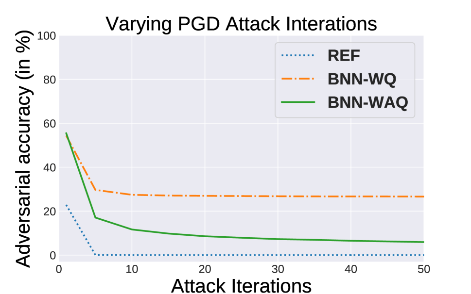
(a) Attack iterations does not improve attack.

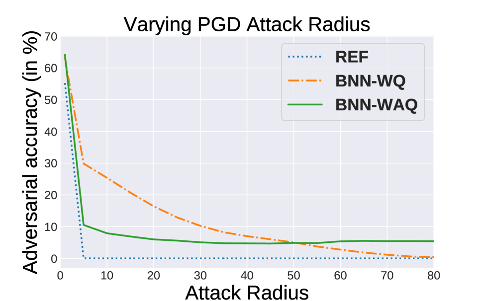
(b) Attack radius does not improve attack.

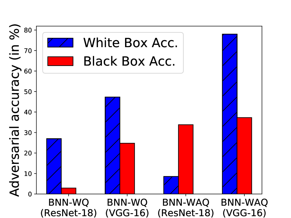
(c) Black-box attacks perform better.

Figure 1: Gradient masking checks in ResNet-18 on CIFAR-10 for pgd attack with $L_{\infty}$ bound. While (a), (c) show signs of gradient masking, (b) does not. We attribute this discrepancy to the random initial step before pgd.

Method	ResNet-18			VGG-16
	Clean	Adv.(1)	Adv.(20)	Clean	Adv.(1)	Adv.(20)
ref	94.46	0.00	0.00	93.31	0.04	0.00
bnn-wq	93.18	26.98	17.91	91.53	47.32	38.49
bnn-waq	87.67	8.57	1.94	89.69	78.01	59.26

Table 1: Clean and adversarial accuracy (PGD attack with $L_{\infty}$ bound) on the test set of CIFAR-10 using ResNet-18 and VGG-16. In brackets, we mention number of random restarts used to perform the attack. Note, bnn s yield higher adversarial accuracy than floating point networks consistently.

Robustness Evaluation of bnn s

We start by evaluating the adversarial accuracy (i.e. accuracy on the perturbed data) of bnn s using the pgd attack with perturbation bound of $8$ pixels (assuming each pixel in the image is in $[0,255]$) with respect to $L_{\infty}$ norm, step size $\eta=2$ and the total number of iterations $T=20$. The attack details are the same in all evaluated settings unless stated otherwise. We perform experiments on CIFAR-10 dataset using ResNet-18 and VGG-16 architectures and report the clean accuracy and pgd adversarial accuracy with 1 and 20 random restarts in Table 1. It can be clearly and consistently observed that binary networks have high adversarial accuracy compared to the floating point counterparts. Even with 20 random restarts, bnn s clearly outperform floating point networks in terms of adversarial accuracy. Since this result is surprising, we investigate this phenomenon further to understand whether bnn s are actually robust to adversarial perturbations or they show a fake sense of security due to obfuscated gradients (Athalye, Carlini, and Wagner 2018).

Identifying Obfuscated Gradients.

Recently, it has been shown that several defense mechanisms intentionally or unintentionally break gradient descent and cause obfuscated gradients and thus exhibit a false sense of security (Athalye, Carlini, and Wagner 2018). Several gradient based adversarial attacks tend to fail to produce adversarial perturbations in scenarios where the gradients are uninformative, referred to as gradient masking. Gradient masking can occur due to shattered gradients, stochastic gradients or exploding and vanishing gradients. We try to identify gradient masking in binary networks based on the empirical checks provided in (Athalye, Carlini, and Wagner 2018). If any of these checks fail, it indicates gradient masking issue in bnn s.

To illustrate this, we analyse the effects of varying different hyperparameters of pgd attack on bnn s trained on CIFAR-10 using ResNet-18 architecture. Even though varying pgd perturbation bound does not show any signs of gradient masking, varying attack iterations and black-box vs white-box results (on ResNet-18 and VGG-16) clearly indicate gradient masking issues as depicted in Fig. 1. The black-box attack outperforming white-box attack for bnn s certainly indicates gradient masking issues since the black-box attack do not use the gradient information from model being attacked. Here, our black-box model to a bnn is the analogous floating point network trained on the same dataset and the attack is the same pgd with $L_{\infty}$ bound.

These checks demonstrate that bnn s are prone to gradient masking and exhibit fake robustness. Note, shattered gradients occur due to non-differentiable components in the defense mechanism and stochastic gradients are caused by randomized gradients. Since bnn s are trainable from scratch and does not have randomized gradients, we narrow down gradient masking issue to vanishing or exploding gradients. Since, vanishing or exploding gradients occur due to poor signal propagation, by introducing a single scalar, we discuss two approaches to mitigate this issue, which lead to almost $100\%$ success rate for gradient based attacks on bnn s.

Signal Propagation of Neural Networks

We first describe how poor signal propagation in neural networks can cause vanishing or exploding gradients. Then we discuss the idea of introducing a single scalar to improve the existing gradient based attacks without affecting the prediction (i.e., decision boundary) of the trained models.

We consider a neural network $f_{\mathbf{w}}$ for an input ${\mathbf{x}}^{0}$, having post-activations ${\mathbf{a}}^{l}$, for $l\in\{1\ldots K\}$ up to $K$ layers and logits ${\mathbf{a}}^{K}=f_{\mathbf{w}}({\mathbf{x}}^{0})$. Now, since softmax cross-entropy is usually used as the loss function, we can write:

$$\ell(\mathbf{a}^{K},\mathbf{y})=-\mathbf{y}^{T}\log(\mathbf{p})\ ,\qquad\mathbf{p}=\operatorname{softmax}(\mathbf{a}^{K})\ ,$$ (3)

where $\mathbf{y}\in\rm I\!R^{d}$ is the one-hot encoded target label and $\log$ is applied elementwise.

For various gradient based adversarial attacks discussed earlier, gradient of the loss $\ell$ is used with respect to the input ${\mathbf{x}}^{0}$, which can also be formulated using chain rule as,

$$\begin{split}\frac{\partial\ell(\mathbf{a}^{K},\mathbf{y})}{\partial{\mathbf{x}}^{0}}=\frac{\partial\ell(\mathbf{a}^{K},\mathbf{y})}{\partial{\mathbf{a}}^{K}}\frac{\partial{\mathbf{a}}^{K}}{\partial{\mathbf{x}}^{0}}=\psi({\mathbf{a}}^{K},{\mathbf{y}})\,{\mathbf{J}}\ ,\end{split}$$ (4)

where $\psi$ denotes the error signal and ${\mathbf{J}}\in\mathbb{R}^{d\times N}$ is the input-output Jacobian. Here we use the convention that $\partial\mathbf{v}/\partial\mathbf{u}$ is of the form $\mathbf{v}$-size $\times$ $\mathbf{u}$-size.

Notice there are two components that influence the gradients, 1) the Jacobian ${\mathbf{J}}$ and 2) the error signal $\psi$. Gradient based attacks would fail if either the Jacobian is poorly conditioned or the error signal has saturating gradients, both of these will lead to vanishing gradients in $\partial\ell/\partial{\mathbf{x}}^{0}$.

The effects of Jacobian on the signal propagation is studied in dynamical isometry and mean-field theory literature (Pennington, Schoenholz, and Ganguli 2017; Saxe, McClelland, and Ganguli 2013) and it is known that a network is said to satisfy dynamical isometry if the singular values of ${\mathbf{J}}$ are concentrated near $1$. Under this condition, error signals $\psi$ backpropagate isometrically through the network, approximately preserving its norm and all angles between error vectors. Thus, as dynamical isometry improves the trainability of the floating point networks, a similar technique can be useful for gradient based attacks as well.

In fact, almost all initialization techniques (e.g., (Glorot and Bengio 2010)) approximately ensures that the Jacobian ${\mathbf{J}}$ is well-conditioned for better trainability and it is hypothesized that approximate isometry is preserved even at the end of the training. But, for bnn s, the weights are constrained to be $\{-1,1\}$ and hence the weight distribution at end of training is completely different from the random initialization. Furthermore, it is not clear that fully-quantized networks can achieve well-conditioned Jacobian, which guided some research activity in utilizing layerwise scalars (either predefined or learned) to improve bnn training (McDonnell 2018; Rastegari et al. 2016). We would like to point out that the focus of this paper is to improve gradient based attacks on already trained bnn s. To this end learning a new scalar to improve signal propagation at each layer is not useful as it can alter the decision boundary of the network and thus cannot be used in practice on already trained model.

Temperature Scaling for better Signal Propagation.

In this paper, we propose to use a single scalar per network to improve the signal propagation of the network using temperature scaling. In fact, one could replace softmax with a monotonic function such that the prediction is not altered, however, we will show in our experiments that a single scalar with softmax has enough flexibility to improve signal propagation and yields almost $100\%$ success rate with pgd attacks. Essentially, we can use a scalar, $\beta>0$ without changing the decision boundary of the network by preserving the relative order of the logits. Precisely, we consider the following:

$$\begin{split}{\mathbf{p}}(\beta)=\operatorname{softmax}(\bar{{\mathbf{a}}}^{K})\ ,\qquad\bar{{\mathbf{a}}}^{K}=\beta\,{\mathbf{a}}^{K}\ .\end{split}$$ (5)

Here, we write the softmax output probabilities $\mathbf{p}$ as a function of $\beta$ to emphasize that they are softmax output of temperature scaled logits. Now since in this context, the only variable is the temperature scale $\beta$, we denote the loss and the error signal as functions of only $\beta$. With this simplified notation the gradient of the temperature scaled loss with respect to the inputs can be written as:

$$\begin{split}\frac{\partial\ell(\beta)}{\partial{\mathbf{x}}^{0}}=\frac{\partial\ell(\beta)}{\partial\bar{{\mathbf{a}}}^{K}}\frac{\partial\bar{{\mathbf{a}}}^{K}}{\partial{\mathbf{a}}^{K}}\frac{\partial{\mathbf{a}}^{K}}{\partial{\mathbf{x}}^{0}}=\psi(\beta)\beta\,{\mathbf{J}}\ .\end{split}$$ (6)

Note that $\beta$ affects the input-output Jacobian linearly while it nonlinearly affects the error signal $\psi$. To this end, we hope to obtain a $\beta$ that ensures the error signal is useful (i.e., not all zero) as well as the Jacobian is well-conditioned to allow the error signal to propagate to the input.

We acknowledge that while one can find a $\beta>0$ to obtain softmax output ranging from a uniform distribution ($\beta=0$) to one-hot vectors ($\beta\to\infty$), $\beta$ only scales the Jacobian. Therefore, if the Jacobian ${\mathbf{J}}$ has zero singular values, our approach has no effect in those dimensions. However, since most of the modern networks consist of ReLU nonlinearities (generally positive homogeneous functions), the effect of a single scalar would be equivalent (ignoring the biases) to having layerwise scalars such as in (McDonnell 2018). Thus, we believe a single scalar is sufficient for our purpose.

Improved Gradients for Adversarial Attacks

Now we discuss strategies to choose a scalar $\beta$ such that the gradients with respect to input are informative. Let us first analyze the effect of $\beta$ on the error signal. To this end,

$$\begin{split}\psi(\beta)=\frac{\partial\ell(\beta)}{\partial{\mathbf{p}}(\beta)}\frac{\partial{\mathbf{p}}(\beta)}{\partial\bar{{\mathbf{a}}}^{K}}=-(\mathbf{y}-\mathbf{p}(\beta))^{T}\ .\end{split}$$ (7)

where $\mathbf{y}$ is the one-hot encoded target label, and $\mathbf{p}(\beta)$ is the softmax output of scaled logits.

For adversarial attacks, we only consider the correctly classified images (i.e., $\operatorname*{argmax}_{j}y_{j}=\operatorname*{argmax}_{j}p_{j}(\beta)$) as there is no need to generate adversarial examples corresponding to misclassified samples. From the above formula, it is clear that when $\mathbf{p}(\beta)$ is one-hot encoding then the error signal is $\bm{0}$. This is one of the reason for vanishing gradient issue in bnn s. Even if this does not happen for a given image, one can increase $\beta\to\infty$ to make this error signal $\bm{0}$. Similarly, when $\mathbf{p}(\beta)$ is the uniform distribution, the norm of the error signal is at the maximum. This can be obtained by setting $\beta=0$. However, this would also make $\partial\ell(\beta)/\partial\mathbf{x}^{0}=\bm{0}$ as the singular values of the input-output Jacobian would all be $0$.

This analysis indicates that the optimal $\beta$ cannot be obtained by simply maximizing the norm of the error signal and we need to balance both the Jacobian as well as the error signal. To summarize, the scalar $\beta$ should be chosen such that the following properties are satisfied:

1. $\|\psi(\beta)\|_{2}>\rho$ for some $\rho>0$.

2. The Jacobian $\beta\,{\mathbf{J}}$ is well-conditioned, i.e., the singular values of $\beta\,{\mathbf{J}}$ is concentrated around $1$.

Network Jacobian Scaling (njs).

We now discuss a straightforward, two-step approach to attain the aforementioned properties. Firstly, to ensure $\beta{\mathbf{J}}$ is well-conditioned, we simply choose $\beta$ to be the inverse of the mean of singular values of ${\mathbf{J}}$. This guarantees that the mean of singular values of $\beta{\mathbf{J}}$ is $1$.

After this scaling, it is possible that the resulting error signal is very small. To ensure that $\|\psi(\beta)\|_{2}>\rho>0$, we ensure that the softmax output $p_{k}(\beta)$ corresponding to the ground truth class $k$ is at least $\rho$ away from $1$. We now state it as a proposition to derive $\beta$ given a lowerbound on $1-p_{k}(\beta)$.

Proposition 1.

Let ${\mathbf{a}}^{K}\in\rm I\!R^{d}$ with $d>1$ and $a^{K}_{1}\geq a^{K}_{2}\geq\ldots\geq a^{K}_{d}$ and $a^{K}_{1}-a^{K}_{d}=\gamma$. For a given ${0<\rho<(d-1)/d}$, there exists a $\beta>0$ such that ${1-\operatorname{softmax}(\beta a^{K}_{1})>\rho}$, then ${\beta<-\log(\rho/(d-1)(1-\rho))/\gamma}$.

Proof.

This is derived via a simple algebraic manipulation of softmax. Please refer to Appendix. ∎

This $\beta$ can be used together with the one computed using inverse of mean Jacobian Singular Values (jsv). We provide the pseudocode for our proposed pgd++ (njs) attack in Section A of Appendix. Similar approach can also be applied for fgsm++. Notice that, this approach is simple and it adds negligible overhead to the standard pgd attacks. However, it has a hand-designed hyperparameter $\rho$. To mitigate this, next we discuss a hyperparameter-free approach to obtain $\beta$.

Hessian Norm Scaling (hns).

We now discuss another approach to obtain informative gradients. Our idea is to maximize the Frobenius norm of the Hessian of the loss with respect to the input, where the intuition is that if the Hessian norm is large, then the gradient $\partial\ell/\partial\mathbf{x}^{0}$ is sensitive to an infinitesimal change in $\mathbf{x}^{0}$. This means, the infinitesimal perturbation in the input is propagated in the forward pass to the last layer and propagated back to the input layer without attenuation (i.e., the returned signal is not zero), assuming there are no randomized or non-differentiable components in the network. This clearly indicates that the network has good signal propagation as well as the error signals are not all zero. This objective can now be written as:

$$\begin{split}\beta^{*}&=\operatorname*{argmax}_{\beta>0}\left\lVert\frac{\partial^{2}\ell(\beta)}{\partial({\mathbf{x}}^{0})^{2}}\right\rVert_{F}\\ &=\operatorname*{argmax}_{\beta>0}\left\lVert\beta\left[\psi(\beta)\frac{\partial{\mathbf{J}}}{\partial{\mathbf{x}}^{0}}+\beta\left(\frac{\partial{\mathbf{p}}(\beta)}{\partial\bar{{\mathbf{a}}}^{K}}{\mathbf{J}}\right)^{T}{\mathbf{J}}\right]\right\rVert_{F}\ .\\[-4.30554pt] \end{split}$$ (8)

The derivation is provided in Appendix. Note, since ${\mathbf{J}}$ does not depend on $\beta$, ${\mathbf{J}}$ and $\partial{\mathbf{J}}/\partial{\mathbf{x}}^{0}$ are computed only once, $\beta$ is optimized using grid search as it involves only a single scalar. In fact, it is easy to see from the above equation that, when the Hessian is maximized, $\beta$ cannot be zero. Similarly, $\psi(\beta)$ cannot be zero because if it is zero, then the prediction ${\mathbf{p}}(\beta)$ is one-hot encoding (Eq. (7)), consequently $\partial\mathbf{p}(\beta)/\partial\bar{\mathbf{a}}^{K}=\bm{0}$ and this cannot be a maximum for the Hessian norm. Hence, this ensures that $\|\psi(\beta^{*})\|_{2}>\rho$ for some $\rho>0$ and $\beta^{*}$ is bounded according to Proposition 1. Therefore, the maximum is obtained for a finite value of $\beta$. Even though, it is not clear how exactly this approach would affect the singular values of the input-output Jacobian ($\beta\,{\mathbf{J}}$), we know that they are finite and not zero.

Furthermore, there are some recent works (Moosavi-Dezfooli et al. 2019; Qin et al. 2019) show that adversarial training makes the loss surface locally linear around the vicinity of training samples and enforcing local linearity constraint on loss curvature can achieve better robust to adversarial attacks. On the contrary, our idea of maximizing the Hessian, i.e., increasing the nonlinearity of $\ell$, could make the network more prone to adversarial attacks and we intend to exploit that. The psuedocode for pgd++ attack with hns is summarized in Section A of Appendix.

Experiments

We evaluate robustness accuracies of bnn s with weight quantized (bnn-wq), weight and activation quantized (bnn-waq), floating point networks (ref). We evaluate our two pgd ++ variants corresponding to hns and njs on CIFAR-10 and CIFAR-100 datasets with multiple network architectures. In order to demonstrate the effectiveness of our proposed variants on adversarially robust models, we also performed comparisons against stronger attacks such as DeepFool (Moosavi-Dezfooli, Fawzi, and Frossard 2016) and Brendel & Bethge Attack (bba) (Brendel et al. 2019) on adversarially trained ref and bnn-wq. We further provide experimental comparisons against more recent gradient based/free attacks (Auto-PGD (Croce and Hein 2020), Square Attack (Andriushchenko et al. 2020)) proposed to alleviate the issue of gradient obfuscation. More analysis on signal propagation issue in bnn s and our variants success in improving it is provided in Section C.5 of Appendix.

	Network	Adversarial Accuracy (%)
		fgsm	fgsm++		pgd ($L_{\infty}$)	pgd++ ($L_{\infty}$)		pgd ($L_{2}$)	pgd++ ($L_{2}$)
			njs	hns		njs	hns		njs	hns
CIFAR-10	ResNet-18	40.49	3.46	2.51	26.98	0.00	0.00	55.68	0.05	0.05
	VGG-16	57.55	4.00	3.43	47.32	0.00	0.00	56.66	0.35	1.32
	ResNet-50	57.62	6.44	5.35	43.14	0.00	0.00	59.11	0.11	0.08
	DenseNet-121	26.80	4.67	4.24	9.11	0.00	0.00	45.78	0.03	0.06
	MobileNet-V2	33.50	6.42	5.42	26.86	0.00	0.00	34.40	0.12	0.09
CIFAR-100	ResNet-18	25.22	14.08	1.80	8.23	2.45	0.00	25.20	6.79	0.26
	VGG-16	19.82	7.98	1.76	17.44	0.88	0.16	16.25	3.17	0.63
	ResNet-50	37.76	16.33	14.17	25.71	2.33	2.73	30.77	7.90	7.41
	DenseNet-121	28.32	12.21	10.86	8.87	1.15	1.09	24.65	4.54	4.16
	MobileNet-V2	12.09	10.18	8.79	1.44	0.57	0.66	6.12	3.39	3.01

Table 2: Adversarial accuracy on the test set for bnn-wq. Both our njs and hns variants consistently outperform original $L_{\infty}$ bounded fgsm and pgd attack, and $L_{2}$ bounded pgd attack.

	Network	Adversarial Accuracy (%)
		fgsm	fgsm++		pgd ($L_{\infty}$)	pgd++ ($L_{\infty}$)		pgd ($L_{2}$)	pgd++ ($L_{2}$)
			njs	hns		njs	hns		njs	hns
ref	ResNet-18	7.62	5.55	5.35	0.00	0.00	0.00	1.12	0.09	0.05
	VGG-16	11.01	10.04	9.66	0.04	0.00	0.00	2.23	0.78	1.10
	ResNet-50	21.64	6.08	5.70	0.69	0.00	0.00	0.37	0.07	0.09
	DenseNet-121	11.40	7.58	7.30	0.00	0.00	0.00	0.65	0.08	0.06
bnn-waq	ResNet-18	40.84	19.46	19.09	8.57	0.03	0.04	25.24	2.33	2.59
	VGG-16	79.92	15.96	15.39	78.01	0.01	0.02	85.62	0.49	0.62
	ResNet-50	33.16	25.89	27.05	0.49	0.23	0.45	19.41	6.68	8.77
	DenseNet-121	37.20	23.89	24.69	0.81	0.10	0.18	48.37	3.72	6.17

Table 3: Adversarial accuracy on the test set of CIFAR-10 for ref and bnn-waq. Both our njs and hns variants consistently outperform original fgsm and pgd ($L_{\infty}/L_{2}$ bounded) attacks.

Network	Adversarial Accuracy (%)
	fgsm	fgsm	fgsm++		pgd	pgd	Deep	bba	pgd++
		$\beta=0.1$	njs	hns		$\beta=0.1$	Fool		njs	hns
ref	62.38	69.52	61.43	61.40	48.73	61.27	51.01	48.43	47.17	48.54
bc	53.91	62.46	52.90	52.27	41.29	54.24	42.65	40.14	39.35	39.34
gd-$\tanh$	56.13	65.06	55.54	54.81	42.77	56.78	44.78	42.94	42.14	42.30
md-$\tanh$-s	55.10	63.42	54.74	53.82	41.34	54.22	43.46	40.69	40.76	40.67

Table 4: Adversarial accuracy on CIFAR-10 with ResNet-18 for adversarially trained ref and bnn-wq using different quantization methods (bc, gd-$\tanh$, md-$\tanh$-s). Our improved attacks are compared against fgsm, pgd ($L_{\infty}$), a heuristic choice of $\beta=0.1$, DeepFool and bba. Albeit on adversarially trained networks, our methods outperform all the comparable methods.

We use state of the art models trained for binary quantization (where all layers are quantized) for our experimental evaluations. We provide adversarial attack parameters used for fgsm/pgd in Table 6 of Appendix and for other attacks, we use default parameters used in Foolbox (Rauber, Brendel, and Bethge 2017). We also provide some other experimental comparisons such as comparisons against combinatorial attack proposed in (Khalil, Gupta, and Dilkina 2019) in the Appendix. For our hns variant, we sweep $\beta$ from a range such that the hessian norm is maximized for each image, as explained in Appendix. For our njs variant, we set the value of $\rho=0.01$. In fact, our attacks are not very sensitive to $\rho$ and we provide the ablation study in the Appendix.

Results

Our comparisons against the original pgd ($L_{2}$/$L_{\infty}$) and fgsm attack for different bnn-wq are reported in Table 2. Our pgd++ variants consistently outperform original pgd on all networks on both datasets. Even being a gradient based attack, our proposed pgd++ ($L_{2}$/$L_{\infty}$) variants can in fact reach adversarial accuracy close to $0$ on CIFAR-10 dataset, demystifying the fake robustness binarized networks tend to exhibit due to poor signal propagation.

Network	Adversarial Accuracy (%)
	fgsm	fgsm	fgsm++		pgd	pgd	apgd	Square	pgd++
		(dlr)	njs	hns		(dlr)		Attack	njs	hns
ref	7.62	19.48	5.55	5.35	0.00	0.00	0.00	0.55	0.00	0.00
bnn-wq	40.49	19.72	3.46	2.51	26.98	0.00	0.00	0.41	0.00	0.00
bnn-waq	40.84	41.78	19.46	19.09	8.57	4.57	6.32	21.45	0.03	0.04
ref ∗	62.38	66.39	61.43	61.40	48.73	49.73	49.00	54.05	47.17	48.54
bnn-wq ∗	55.10	59.14	54.74	53.82	41.34	41.42	40.85	46.67	40.76	40.67

Table 5: Adversarial accuracy for ref, bnn-wq, and bnn-waq trained on CIFAR-10 using ResNet-18. Here ^∗ denotes adversarially trained models. Both our njs and hns variants consistently outperform $L_{\infty}$ bounded fgsm, pgd and Auto-pgd (apgd) (Croce and Hein 2020) attack performed using Difference of Logits Ratio (dlr)loss and a gradient free attack namely, Square Attack (Andriushchenko et al. 2020) under $L_{\infty}$ bound (8/255). Notice, fgsm, pgd and apgd attack with dlr loss and Square Attack perform even worse than their original form on adversarially trained models in most cases.

Similarly, for one step fgsm attack, our modified versions outperform original fgsm attacks by a significant margin consistently for both datasets on various network architectures. We would like to point out such an improvement in the above two attacks is considerably interesting, knowing the fact that fgsm, pgd with $L_{\infty}$ attacks only use the sign of the gradients so improved performance indicates, our temperature scaling indeed makes some zero elements in the gradient nonzero. We would like to point out here that one can use several random restarts to increase the success rate of original form of fgsm/pgd attack further but to keep comparisons fair we use single random restart for both original and modified attacks. Nevertheless, as it has been observed in Table 1 even with 20 random restarts pgd adversarial accuracies for bnn s cannot reach zero, whereas our proposed pgd++ variants consistently achieve perfect success rate.

The adversarial accuracies of ref and bnn-waq trained on CIFAR-10 using ResNet-18/50, VGG-16 and DenseNet-121 for our variants against original counterparts are reported in Table 3. Overall, for both ref and bnn-waq, our variants outperform the original counterparts consistently. Particularly interesting, pgd++ variants improve the attack success rate on ref networks. This effectively expands the applicability of our pgd++ variants and encourages to consider signal propagation of any trained network to improve gradient based attacks. pgd++ with $L_{\infty}$ variants achieve near-perfect success rate on all bnn-waq s, again validating the hypotheses of fake robustness of bnn s.

To further demonstrate the efficacy of proposed attack variants, we first adversarially trained the bnn-wq s (quantized using bc (Courbariaux, Bengio, and David 2015), gd-$\tanh$/md-$\tanh$-s (Ajanthan et al. 2021)) and floating point networks in a similar manner as in (Madry et al. 2017), using $L_{\infty}$ bounded pgd with $T=7$ iterations, $\eta=2$ and $\epsilon=8$. We report the adversarial accuracies of $L_{\infty}$ bounded attacks and our variants on CIFAR-10 using ResNet-18 in Table 4. These results further strengthens the usefulness of our proposed pgd++ variants. Moreover, with a heuristic choice of $\beta=0.1$ to scale down the logits before performing gradient based attacks performs even worse. Finally, even against stronger attacks (DeepFool, bba) under the same $L_{\infty}$ perturbation bound, our variants outperform consistently on these adversarially trained models in Table 4. We would like to point out that our variants have negligible computational overhead over the original gradient based attacks, whereas stronger attacks are much slower in practice requiring 100-1000 iterations with an adversarial starting point (instead of random initial perturbation).

To illustrate the effectiveness of our proposed variants in improving signal propagation, we compare against gradient based attacks performed using recently proposed Difference of Logits Ratio (dlr)loss (Croce and Hein 2020) that aims to avoid the issue of saturating error signals. Also, we provide comparisons against recently introduced Auto-pgd (apgd)attack performed using dlr loss and a gradient free attack namely, Square Attack (Andriushchenko et al. 2020). We show these experimental comparisons performed on ResNet-18 models trained on CIFAR-10 dataset in Table 5. The attack parameters are same as used for the other experiments. It can be observed that our proposed variants perform better than both pgd or apgd with dlr loss and Square Attack, consistently achieving 0% adversarial accuracy. Infact, much computationally expensive Square attack is unable to achieve 0% adversarial accuracy in any of the cases under the enforced $L_{\infty}$ bound. The margin of difference is significant in case of fgsm attack and adversarial trained models. Infact, it is important to note that gradient based attacks with dlr loss and Square Attack perform worse on adversarially trained models than the original gradient based attacks.

ImageNet.

For other large scale datasets such as ImageNet, BNNs are hard to train with full binarization of parameters and result in poor performance. Thus, most existing works (Yang et al. 2019) on bnn s keep the first and the last layers floating point and introduce several layerwise scalars to achieve good results on ImageNet. In such experimental setups, according to our experiments, trained BNNs do not exhibit gradient masking issues or poor signal propagation and thus are easier to attack using original fgsm/pgd attacks with complete success rate. In such experiments, our modified versions perform equally well compared to the original forms of these attacks.

Related Work

Adversarial examples are first observed in (Szegedy et al. 2014) and subsequently efficient gradient based attacks such as fgsm (Goodfellow, Shlens, and Szegedy 2014) and pgd (Madry et al. 2017) are introduced. There exist recent stronger attacks such as (Moosavi-Dezfooli, Fawzi, and Frossard 2016; Carlini and Wagner 2017; Yao et al. 2019; Finlay, Pooladian, and Oberman 2019; Brendel et al. 2019), however, compared to pgd, they are much slower to be used for adversarial training in practice. For a comprehensive survey related to adversarial attacks, we refer the reader to (Chakraborty et al. 2018).

Some recent works focus on the adversarial robustness of bnn s (Bernhard, Moellic, and Dutertre 2019; Sen, Ravindran, and Raghunathan 2020; Galloway, Taylor, and Moussa 2018; Khalil, Gupta, and Dilkina 2019; Lin, Gan, and Han 2019), however, a strong consensus on the robustness properties of quantized networks is lacking. In particular, while (Galloway, Taylor, and Moussa 2018) claims parameter quantized networks are robust to gradient based attacks based on empirical evidence, (Lin, Gan, and Han 2019) shows activation quantized networks are vulnerable to such attacks and proposes a defense strategy assuming the parameters are floating-point. Differently, (Khalil, Gupta, and Dilkina 2019) proposes a combinatorial attack hinting that activation quantized networks would have obfuscated gradients issue. Though as shown in the paper, the combinatorial attack is not scalable and thus experiments were shown on only few layered MLPs trained on MNIST. (Sen, Ravindran, and Raghunathan 2020) shows ensemble of mixed precision networks to be more robust than original floating point networks; however (Tramer et al. 2020) later shows the presented defense method can be attacked with minor modification in the loss function. In short, although it has been hinted that there maybe gradient masking in bnn s (especially in activation quantized networks), a thorough understanding is lacking on whether bnn s are robust, if not what is the reason for the failure of most commonly used gradient based attacks on binary networks. We answer this question in this paper and introduce improved gradient based attacks.

Conclusion

In this work, we have shown that both bnn-wq and bnn-waq tend to show a fake sense of robustness on gradient based attacks due to poor signal propagation. To tackle this issue, we introduced our two variants of pgd++ attack, namely njs and hns. Our proposed pgd++ variants not only possess near-complete success rate on binarized networks but also outperform standard $L_{\infty}$ and $L_{2}$ bounded pgd attacks on floating point networks. We finally show improvement in attack success on adversarially trained ref and bnn-wq against stronger attacks (DeepFool and bba).

Appendix

Here, we first provide the pseudocodes, proof of the proposition and the derivation of Hessian. Later we give additional experiments, analysis and the details of our experimental setting.

Appendix A Pseudocode

We provide pseudocode for pgd++ with njs in Algorithm 1 and pgd++ with hns in Algorithm 2.

1:$T,\epsilon,\eta,\rho,{\mathbf{x}}^{0},{\mathbf{y}},k$

2:$\|{\mathbf{x}}^{T+1}-{\mathbf{x}}^{0}\|_{\infty}\leq\epsilon$

3:$\beta_{1}=(M\,d)/\big{(}\sum_{i=1}^{M}\sum_{j=1}^{d}\mu_{j}({\mathbf{J}}_{i})\big{)}$ $\triangleright$ $\beta_{1}$ computed using Network Jacobian.

4:${\mathbf{x}}^{1}=P_{\infty}^{\epsilon}({\mathbf{x}}^{0}+\mbox{Uniform}(-1,1))$ $\triangleright$ Random Initialization with Projection

5:for $t\leftarrow 1,\dots T$ do

6:     $\beta_{2}=1.0$

7:     ${\mathbf{p}}^{\prime}=\operatorname{softmax}(\beta_{1}(f_{{\mathbf{w}}^{*}}({\mathbf{x}}^{t})))$

8:     if $1-p^{\prime}_{k}\leq\rho$ then $\triangleright$ $\rho=0.01$

9:         $\beta_{2}=-\log(\rho/(d-1)(1-\rho))/\gamma$ $\triangleright$ $\gamma$ computed using Proposition 2      

10:     $\ell=-{\mathbf{y}}^{T}\log(\operatorname{softmax}(\beta_{2}\beta_{1}(f_{{\mathbf{w}}^{*}}({\mathbf{x}}^{t}))))$

11:     ${\mathbf{x}}^{t+1}=P_{\infty}^{\epsilon}({\mathbf{x}}^{t}+\eta\operatorname{sign}(\nabla_{\mathbf{x}}\ell(\mathbf{x}^{t})))$ $\triangleright$ Update Step with Projection

Algorithm 1 pgd++ with njs with $L_{\infty}$, $T$ iterations, radius $\epsilon$, step size $\eta$, network $f_{{\mathbf{w}}^{*}}$, input ${\mathbf{x}}^{0}$, label $k$, one-hot ${\mathbf{y}}\in\{0,1\}^{d}$, gradient threshold $\rho$.

1:$T,\epsilon,\eta,{\mathbf{x}}^{0},{\mathbf{y}},k$

2:$\|{\mathbf{x}}^{T+1}-{\mathbf{x}}^{0}\|_{\infty}\leq\epsilon$

3:${\mathbf{x}}^{1}=P_{\infty}^{\epsilon}({\mathbf{x}}^{0}+\mbox{Uniform}(-1,1))$ $\triangleright$ Random Initialization with Projection

4:$\beta^{*}=\operatorname*{argmax}_{\beta>0}\left\lVert\partial^{2}\ell(\beta)/\partial({\mathbf{x}}^{0})^{2}\right\rVert_{F}$ $\triangleright$ Grid Search

5:for $t\leftarrow 1,\dots T$ do

6:     $\ell=-{\mathbf{y}}^{T}\log(\operatorname{softmax}(\beta^{*}(f_{{\mathbf{w}}^{*}}({\mathbf{x}}^{t}))))$

7:     ${\mathbf{x}}^{t+1}=P_{\infty}^{\epsilon}({\mathbf{x}}^{t}+\eta\operatorname{sign}(\nabla_{\mathbf{x}}\ell(\mathbf{x}^{t})))$ $\triangleright$ Update Step with Projection

Algorithm 2 pgd ++ with hns with $L_{\infty}$, $T$ iterations, radius $\epsilon$, step size $\eta$, network $f_{{\mathbf{w}}^{*}}$, input ${\mathbf{x}}^{0}$, label $k$, one-hot ${\mathbf{y}}\in\{0,1\}^{d}$, gradient threshold $\rho$.

Appendix B Derivations

B.1  Deriving $\beta$ given a lowerbound on $1-p_{k}(\beta)$

Proposition 2.

Let ${\mathbf{a}}^{K}\in\rm I\!R^{d}$ with $d>1$ and $a^{K}_{1}\geq a^{K}_{2}\geq\ldots\geq a^{K}_{d}$ and $a^{K}_{1}-a^{K}_{d}=\gamma$. For a given ${0<\rho<(d-1)/d}$, there exists a $\beta>0$ such that ${1-\operatorname{softmax}(\beta a^{K}_{1})>\rho}$, then ${\beta<-\log(\rho/(d-1)(1-\rho))/\gamma}$.

Proof.

Assuming $a^{K}_{1}-a^{K}_{d}=\gamma$, we derive a condition on $\beta$ such that ${1-\operatorname{softmax}(\beta a^{K}_{1})>\rho}$.

$$1-\operatorname{softmax}(\beta a^{K}_{1}) >\rho\ ,$$ (9)

$$\operatorname{softmax}(\beta a^{K}_{1}) <1-\rho\ ,$$

$$\exp(\beta a^{K}_{1})/\sum_{\lambda=1}^{d}\exp(\beta a^{K}_{\lambda}) <1-\rho\ ,$$

$$1/\big{(}1+\sum_{\lambda=2}^{d}\exp(\beta(a^{K}_{\lambda}-a^{K}_{1}))\big{)} <1-\rho\ .$$

Since, $a^{K}_{1}-a^{K}_{\lambda}\leq\gamma$ for all $\lambda>1$,

$$1/\big{(}1+\sum_{\lambda=2}^{d}\exp(\beta(a^{K}_{\lambda}-a^{K}_{1}))\big{)}\leq 1/\big{(}1+\sum_{\lambda=2}^{d}\exp(-\beta\gamma)\big{)}\ .$$ (10)

Therefore, to ensure $1/\big{(}1+\sum_{\lambda=2}^{d}\exp(\beta(a^{K}_{\lambda}-a^{K}_{1}))\big{)}<1-\rho$, we consider,

$$1/\big{(}1+\sum_{\lambda=2}^{d}\exp(-\beta\gamma)\big{)} <1-\rho\ ,\quad\mbox{$a^{K}_{1}-a^{K}_{\lambda}\leq\gamma$ for all $\lambda>1$}\ ,$$ (11)

$$1/\big{(}1+(d-1)\exp(-\beta\gamma)\big{)} <1-\rho\ ,$$

$$\exp(-\beta\gamma) >\rho/(d-1)(1-\rho)\ ,$$

$$-\beta\gamma >\log(\rho/(d-1)(1-\rho))\ ,\quad\mbox{$\exp$ is monotone}\ ,$$

$$\beta <-\log(\rho/(d-1)(1-\rho))/\gamma\ .$$

Therefore for any ${\beta<-\log(\rho/(d-1)(1-\rho))/\gamma}$, the above inequality
$1-\operatorname{softmax}(\beta a^{K}_{1})>\rho$ is satisfied. ∎

B.2  Derivation of Hessian

We now derive the Hessian of the input mentioned in Eq. (8) of the paper. The input gradients can be written as:

$$\frac{\partial\ell(\beta)}{\partial{\mathbf{x}}^{0}}=\frac{\partial\ell(\beta)}{\partial{\mathbf{p}}(\beta)}\frac{\partial{\mathbf{p}}(\beta)}{\partial\bar{{\mathbf{a}}}^{K}(\beta)}\beta{\mathbf{J}}=\psi(\beta)\beta{\mathbf{J}}\ .$$ (12)

Now by product rule of differentiation, input hessian can be written as:

$$\frac{\partial^{2}\ell(\beta)}{\partial({\mathbf{x}}^{0})^{2}} =\beta\left[\psi(\beta)\frac{\partial{\mathbf{J}}}{\partial{\mathbf{x}}^{0}}+\left(\frac{\partial\psi(\beta)}{\partial{\mathbf{x}}^{0}}\right)^{T}{\mathbf{J}}\right]\ ,$$ (13)

$$=\beta\left[\psi(\beta)\frac{\partial{\mathbf{J}}}{\partial{\mathbf{x}}^{0}}+\left(\frac{\partial{\mathbf{p}}(\beta)}{\partial{\mathbf{x}}^{0}}\right)^{T}{\mathbf{J}}\right]\ ,\quad\psi(\beta)=-({\mathbf{y}}-{\mathbf{p}}(\beta))^{T}\ ,$$

$$=\beta\left[\psi(\beta)\frac{\partial{\mathbf{J}}}{\partial{\mathbf{x}}^{0}}+\beta\left(\frac{\partial{\mathbf{p}}(\beta)}{\partial\bar{{\mathbf{a}}}^{K}}{\mathbf{J}}\right)^{T}{\mathbf{J}}\right]\ .$$

Appendix C Additional Experiments

In this section we first provide more experimental details and then some ablation studies.

C.1  Experimental Details

We first mention the hyperparameters used to perform fgsm and pgd attack for all the experiments in the paper in Table 6. To make a fair comparison, we keep the attack parameters same for our proposed variants of fgsm++ and pgd++ attacks. In our experiments we found that increasing attack iterations, attack radius and step size does not yield better success rate for original gradient based attacks thus we used these standard attack parameters. For attacks under $L_{2}$ bound, we use attack parameters similar to (Finlay, Pooladian, and Oberman 2019). All our experiments are performed using single NVIDIA Tesla P100 GPUs. We also perform multiple runs for achieving trained bnn s and the performance change remains $\leq 0.3\%$ reflecting the significance of improvement in our attack success rates.

Dataset	Attack	$\epsilon$	$\eta$	$T$
CIFAR-10	fgsm	8	8	1
	pgd ($L_{\infty}$)	8	2	20
	pgd ($L_{2}$)	120	15	20
CIFAR-100	fgsm	4	4	1
	pgd ($L_{\infty}$)	4	1	10
	pgd ($L_{2}$)	60	15	10

Table 6: Attack parameters ($\epsilon$ & $\eta$ in pixels).

For pgd++ with hns variant, we maximize Frobenius norm of Hessian with respect to the input as specified in Eq. (8) of the paper by grid search for the optimum $\beta$. We would like to point out that since only $\psi(\beta)$ and ${\mathbf{p}}(\beta)$ terms are dependent on $\beta$, we do not need to do forward and backward pass of the network multiple times during the grid search. This significantly reduces the computational overhead during the grid search. We can simply use the same network outputs ${\mathbf{a}}^{K}$ and network jacobian ${\mathbf{J}}$ (as computed without using $\beta$) for the grid search, while computing the other terms at each iteration of grid search. We apply grid search to find the optimum beta between $100$ equally spaced intervals of $\beta$ starting from $\beta_{1}$ to $\beta_{2}$. Here, $\beta_{1}$ and $\beta_{2}$ are computed based on Proposition 1 in the paper where $\rho=1e-72$ and $\rho=1-(1/d)-(1e-2)$ respectively, where $d$ is number of classes and $\gamma=a_{1}^{K}-a_{2}^{K}$ so that $1-\operatorname{softmax}(\beta a_{1}^{K})<\rho$. Also, note that we estimate the optimum $\beta$ for each test sample only at the start of the first iteration of an iterative attack and then use the same $\beta$ for the next iterations.

Computational Overhead of njs and hns.

Our Jacobian calculation takes just a single backward pass through the network and thus adds a negligible overhead. Our njs approach for scaling estimates $\beta$ as inverse of mean jsv using $100$ random test samples, which is similar to $100$ backward passes. The computation overhead of hns is roughly comprised of a full backward pass through the network for estimating the Jacobian and grid search for finding optimal $\beta$.

fgsm	fgsm++ (njs)	fgsm++ (hns)
0.01492	0.01604	0.0932

Table 7: Comparisons of computational cost in seconds between fgsm and fgsm++ to generate one adversarial sample using different methods. Note, that both variants take less than 0.1 second which is significantly faster than stronger attacks mentioned in Table 4 and 5 of the main paper.

For hns variant, we maximize the Frobenius norm of the Hessian as specified in Eq. (8) of the paper by grid search to find the optimum $\beta$. First of all, we are computing the Hessian w.r.t. input (dimension in thousands), this is significantly cheaper than Hessian w.r.t. network parameters (dimension in millions). Furthermore, in Eq. (8), ${\mathbf{J}}$ does not depend on $\beta$, therefore ${\mathbf{J}}$ and $\partial{\mathbf{J}}/\partial{\mathbf{x}}^{0}$ are computed only once during the grid search and re-used for each iteration of grid search. This significantly reduces the computational overhead. Our Jacobian calculation takes just a single full backward pass through the network (using parallel compute), thus adds negligible overhead. Moreover, for piecewise linear networks (e.g., ReLU activations), $\partial{\mathbf{J}}/\partial{\mathbf{x}}^{0}=0$ almost everywhere (Yao et al. 2018). We provide computational time comparisons for original fgsm and fgsm++ using njs and hns on ResNet-18 using CIFAR-10 in Table 7. These experiments are performed on NVIDIA GeForce RTX 2080 GPUs at a batchsize of $1$. Note, that our implementation of sequential grid search with $100$ intervals can be parallelized to speed up hns further.

C.2  Comparisons against Auto-pgd attack, gradient free attack and Combinatorial attack

We also compared our proposed pgd++ variants against recently proposed Auto-pgd (apgd)with Difference of Logits Ratio (dlr)loss (Croce and Hein 2020) and gradient free Square Attack (Andriushchenko et al. 2020) on different networks trained using VGG-16 on CIFAR-10 dataset and the results are reported in Table 8. The attack parameters for this experiment are the same as reported in the paper. It can be clearly seen that our proposed variants perform better than both apgd with dlr loss and Square Attack, consistently achieving 0% adversarial accuracy. Infact, much computationally expensive Square attack is unable to achieve 0% adversarial accuracy in any of the cases under the enforced $L_{\infty}$ bound.

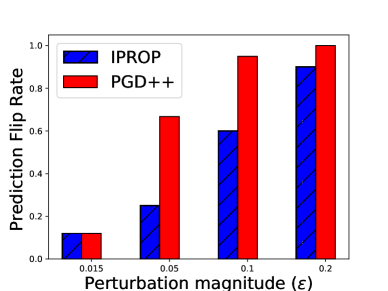
Figure 2: Classification flip rate (higher the better) using pgd++ (njs) attack and IPROP (Khalil, Gupta, and Dilkina 2019) on MLP trained on MNIST dataset under various $L_{\infty}$ bound. Notice, pgd++ attack consistently flips the predicition more times than IPROP under different perturbation magnitudes.

We provide comparisons against combinatorial attack designed for quantized networks proposed in (Khalil, Gupta, and Dilkina 2019). Since their proposed attack namely iprop is not scalable for deep neural networks and was thus tested on MLPs trained on MNIST dataset. We follow their experimental protocol with a bnn-waq using MLP (5 hidden layer with 100 units each) trained on MNIST dataset achieving 95% classification accuracy. We provide the proportion of examples where iprop and pgd++ (njs) attack is able to flip the classification in Fig. 2 under different $L_{\infty}$ perturbation bounds in range $[0,1]$. Our pgd++ variant performs consistently better than iprop under different perturbation magnitudes, clearly reflecting efficacy of pgd++ despite being simple modification over pgd.

Method	apgd	Square	pgd++
		Attack	njs	hns
ref	0.79	2.25	0.00	0.00
bnn-wq	8.23	1.98	0.00	0.00
bnn-waq	0.38	16.67	0.01	0.02

Table 8: Adversarial accuracy for ref, bnn-wq and bnn-waq trained on CIFAR-10 using VGG-16. Both our njs and hns variants consistently outperform Auto-pgd (apgd) (Croce and Hein 2020) performed using Difference of Logits Ratio (dlr)loss and a gradient free attack namely, Square Attack (Andriushchenko et al. 2020) under $L_{\infty}$ bound (8/255).

C.3  Other Experiments

Network	Adversarial Accuracy (%)
	fgsm	fgsm++		pgd ($L_{\infty}$)	pgd++ ($L_{\infty}$)		pgd ($L_{2}$)	pgd++ ($L_{2}$)
		njs	hns		njs	hns		njs	hns
ResNet-18	9.06	9.23	2.70	0.14	0.14	0.00	4.86	0.17	0.15
VGG-16	16.28	17.24	9.19	1.53	0.95	0.25	4.87	1.50	1.38
ResNet-50	12.95	12.95	11.94	0.12	0.00	0.00	10.50	4.43	4.14
DenseNet-121	11.41	11.41	10.74	0.00	0.00	0.00	4.32	3.09	2.76

Table 9: Adversarial accuracy on the test set of CIFAR-100 for ref (floating point networks). Both our njs and hns variants consistently outperform original fgsm and pgd ($L_{\infty}/L_{2}$ bounded) attacks.

Network	pgd	Deep	bba	pgd++
		Fool		njs	hns
ResNet-18	8.57	18.92	0.81	0.03	0.04
VGG-16	78.01	12.12	0.10	0.01	0.02

Table 10: Adversarial accuracy on the test set of CIFAR-10 for bnn-waq. Here, we compare our proposed variants against much stronger attacks namely DeepFool (Moosavi-Dezfooli, Fawzi, and Frossard 2016) and bba (Brendel et al. 2019). Both our variants outperform stronger attacks. Note, DeepFool and bba are much slower in practise requiring 100-1000 iterations. bba specifically requires even an adversarial start point that needs to be computed using another adversarial attack.

We provide adversarial accuracy comparisons for different attack methods on CIFAR-100 using ResNet-18, VGG-16, ResNet-50 and DenseNet-121 in Table 9. Again similar to the results in the paper, our proposed pgd++ and fgsm++ outperform original form of pgd and fgsm consistently in all the experiments on floating point networks. We also provide adversarial accuracy comparison of our proposed variants against stronger attacks namely DeepFool (Moosavi-Dezfooli, Fawzi, and Frossard 2016) and bba (Brendel et al. 2019) on bnn-waq trained on CIFAR-10 dataset in Table 10. In this experiment, our proposed variants again outperform even the stronger attacks which take 100-1000 iterations with adversarial start point (instead of random initial perturbation). It should be noted that although bba performs much better than DeepFool and pgd, it still has inferior success rate than ours considering the fact that it takes multiple hours to run bba whereas our proposed variants are almost as efficient as pgd attack.

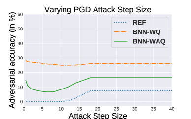
Figure 3: Adversarial accuracy using pgd attack under $L_{\infty}$ bound (8/255) with varying step size ($\eta$) on ResNet-18 trained on CIFAR-10. Notice, pgd attack is unable to reach zero adversarial accuacy for bnn s with any step size.

Step Size Tuning for pgd attack.

We would like to point out that step size $\eta$ and temperature scale $\beta$ have different effects in the attacks performed. Notice, pgd and fgsm attack under $L_{\infty}$ bound only use the sign of input gradients in each gradient ascent step. Thus, if the input gradients are completely saturated (which is the case for bnn s), original forms of pgd or fgsm will not work irrespective of the step size used. To illustrate this, we performed extensive step size tuning for original form of pgd attack on different ResNet-18 models trained on CIFAR-10 dataset and the adversarial accuracies are reported in Fig. 3. It can be observed clearly that although tuning the step size lowers adversarial accuracy a bit in some cases but still cannot reach zero for bnn s unlike our proposed variants.

Adversarial training using pgd++.

We also investigate the potential application of pgd++ for adversarial training to improve the robustness of neural networks. pgd++ attack is most effective when applied to a network with poor signal propagation. However, adversarial training is performed from random initialization (Glorot and Bengio 2010) exhibiting good signal propagation. Thus, pgd and pgd++ perform similarly for adversarial training. We infer these conclusions from our experiments on adversarial training using pgd++.

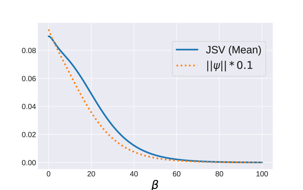
(a)

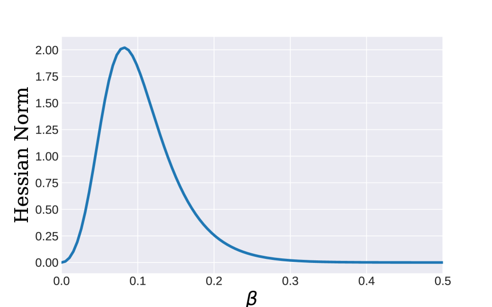
(b)

Figure 4: Plots to show how variation in $\beta$ affects jacobian, error signal and hessian. (a) Error signal $(\psi(\beta))$ and Jacobian of softmax $(\partial{\mathbf{p}}(\beta)/\partial\bar{{\mathbf{a}}}^{K})$ vs. $\beta$ for a random correctly classified logits. Notice that, $\psi(\beta)$ and mean jsv of $\partial{\mathbf{p}}(\beta)/\partial\bar{{\mathbf{a}}}^{K}$ behave similarly. (b) Hessian norm vs. $\beta$ on a random correctly classified image. The plot clearly shows a concave behaviour and the maximum point occurs at a small value where both $\psi(\beta)$ and $\partial{\mathbf{p}}(\beta)/\partial\bar{{\mathbf{a}}}^{K}$ are non zero.

	Original	Heuristic	njs	hns
bnn-wq	0.8585	0.8845	0.4139	0.3450
bnn-waq	0.7239	3.1578	0.3120	0.2774

Table 11: clever Scores (Weng et al. 2018) for bnn-wq and bnn-waq trained on CIFAR-10 using ResNet-18. We compare CLEVER Scores returned for $L_{1}$ norm perturbation using different ways of temperature scaling applied. Here, Original refers to original network without temperature scaling and Heuristic denotes temperature scale with small $\beta=0.01$.

clever Scores.

Recently clever Scores (Weng et al. 2018) have been proposed as an empirical estimate to measure robustness lower bounds for deep networks. It has been later shown that gradient masking issues cause clever to overestimate the robustness bounds (Goodfellow 2018). Here we try to improve the clever scores using different ways of choosing $\beta$ in temperature scaling. For this experiment, we use clever implementation of Adversarial Training Toolbox (Nicolae et al. 2018). We set number of batches to 50, batch size to 10, radius to 5, and chose $L_{1}$ norm as hyperparameters (based on the (Weng et al. 2018)). We compare our variants namely njs and hns against heuristic choice of small $\beta=0.01$ and original clever Scores for bnn-wq and bnn-waq (trained on CIFAR-10 using ResNet-18) in Table 11. It can be clearly seen that our proposed variants improve the robustness bounds computed using clever whereas a heuristic choice of $\beta=0.01$ performs even worse.

C.4  Stability of pgd++ with njs with variations in $\rho$

We perform ablation studies with varying $\rho$ for pgd++ with njs in Table 12 for CIFAR-10 dataset using ResNet-18 architecture. It clearly illustrates that our njs variant is quite robust to the choice of $\rho$ as we are able to achieve near perfect success rate with pgd++ with different values of $\rho$. As long as value of $\rho$ is large enough to avoid one-hot encoding on softmax outputs (in turn avoid $\|\psi(\beta)\|$ to be zero) of correctly classified sample, our approach with njs variant is quite stable.

Methods	pgd++ (njs) - Varying $\rho$
	$1e-05$	$1e-04$	$1e-03$	$1e-02$	$1e-01$	$2e-01$
ref	0.00	0.00	0.00	0.00	0.00	0.00
bnn-wq	0.00	0.00	0.00	0.00	0.00	0.00
bnn-waq	0.15	0.08	0.04	0.03	0.04	0.02

Table 12: Adversarial accuracy on the test set for binary neural networks using $L_{\infty}$ bounded pgd++ attack using njs with varying $\rho$. For different values of $\rho$, our approach is quite stable.

C.5  Signal Propagation and Input Gradient Analysis using njs and hns

We first provide plots to to show how jacobian, error signal and hessian norm are influenced by $\beta$ in Fig. 4. We then provide an example illustration in Fig. 5 to better understand how the input gradient norm i.e., $\|\partial\ell(\beta)/\partial{\mathbf{x}}^{0}\|_{2}$, and norm of sign of input gradient, i.e., $\|\text{sign}(\partial\ell(\beta)/\partial{\mathbf{x}}^{0})\|_{2}$ is influenced by $\beta$. It clearly shows that both the plots have a concave behavior where an optimal $\beta$ can maximize the input gradient. Also, it can be quite evidently seen in Fig. 5 (b) that within an optimal range of $\beta$, gradient vanishing issue can be avoided. If $\beta\to 0$ or $\beta\to\infty$, it changes all the values in input gradient matrix to zero and inturn $\|\text{sign}(\partial\ell(\beta)/\partial{\mathbf{x}}^{0})\|_{2}=0$.

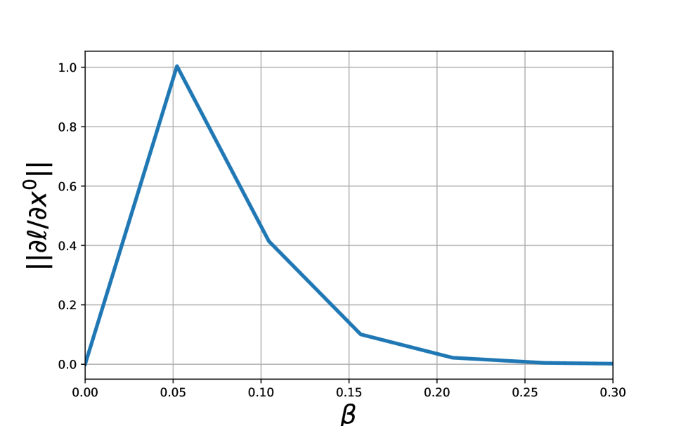
(a)

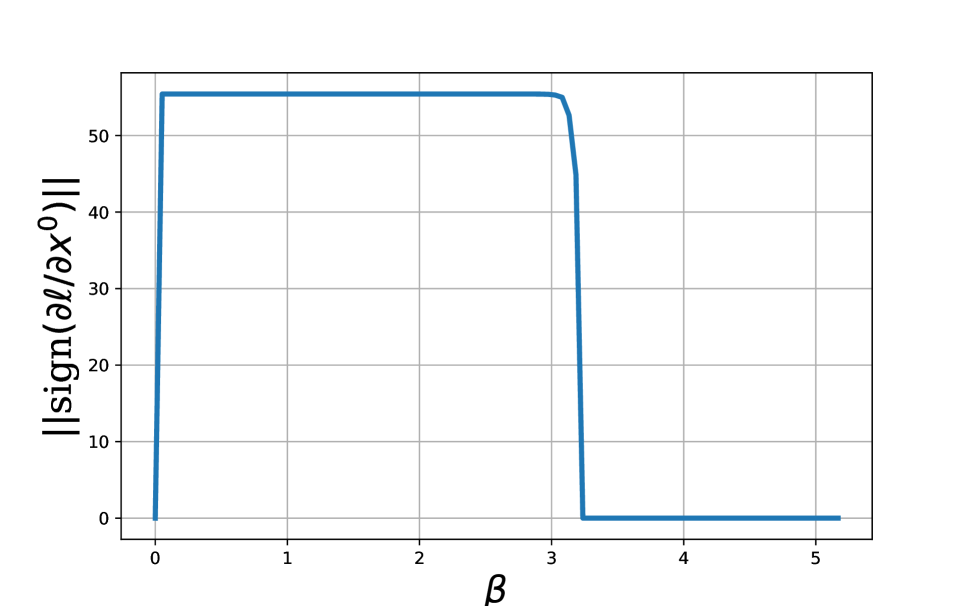
(b)

Figure 5: Plots to show how variation in $\beta$ affects (a) norm of input gradient, i.e., $\|\partial\ell(\beta)/\partial{\mathbf{x}}^{0}\|_{2}$, (b) norm of sign of input gradient, i.e., $\|\text{sign}(\partial\ell(\beta)/\partial{\mathbf{x}}^{0})\|_{2}$ on a random correctly classified image. Notice that, both input gradient and signed input gradient norm behave similarly, showing a concave behaviour. This plot is computed for bnn-wq network on CIFAR-10, ResNet-18. (b) clearly illustrates how optimum $\beta$ can avoid vanishing gradient issue since $\|\mbox{sign}(\partial\ell(\beta)/\partial{\mathbf{x}}^{0})\|_{2}$ will only be zero if input gradient matrix has only zeros.

Methods		ref	Adv. Train	bnn-wq	bnn-waq
jsv (Mean)	Orig.	$8.09\mathrm{e}{+00}$	$5.15\mathrm{e}{-01}$	$3.53\mathrm{e}{+01}$	$1.11\mathrm{e}{+00}$
	njs	$9.51\mathrm{e}{-01}$	$5.70\mathrm{e}{-01}$	$9.95\mathrm{e}{-01}$	$2.24\mathrm{e}{-01}$
	hns	$2.38\mathrm{e}{+00}$	$6.11\mathrm{e}{+00}$	$1.19\mathrm{e}{+01}$	$4.65\mathrm{e}{+00}$
jsv (Std.)	Orig.	$6.27\mathrm{e}{+00}$	$4.10\mathrm{e}{-01}$	$3.53\mathrm{e}{+01}$	$1.97\mathrm{e}{+00}$
	njs	$7.58\mathrm{e}{-01}$	$6.34\mathrm{e}{-01}$	$9.71\mathrm{e}{-01}$	$6.73\mathrm{e}{-01}$
	hns	$4.41\mathrm{e}{+00}$	$5.34\mathrm{e}{+02}$	$2.13\mathrm{e}{+02}$	$1.24\mathrm{e}{+02}$
$\boldsymbol{\|\psi\|_{2}}$	Orig.	$9.08\mathrm{e}{-03}$	$2.33\mathrm{e}{-01}$	$6.20\mathrm{e}{-03}$	$9.46\mathrm{e}{-03}$
	njs	$4.66\mathrm{e}{-01}$	$2.35\mathrm{e}{-01}$	$5.37\mathrm{e}{-01}$	$1.20\mathrm{e}{-01}$
	hns	$1.48\mathrm{e}{-01}$	$2.57\mathrm{e}{-01}$	$2.07\mathrm{e}{-01}$	$2.44\mathrm{e}{-01}$
$\boldsymbol{\|\partial\ell/\partial{\mathbf{x}}^{0}\|_{2}}$	Orig.	$2.42\mathrm{e}{-01}$	$8.52\mathrm{e}{-02}$	$2.27\mathrm{e}{-01}$	$6.33\mathrm{e}{-02}$
	njs	$9.52\mathrm{e}{-01}$	$1.10\mathrm{e}{-01}$	$8.91\mathrm{e}{-01}$	$1.24\mathrm{e}{-01}$
	hns	$7.49\mathrm{e}{-01}$	$8.18\mathrm{e}{-01}$	$3.70\mathrm{e}{-01}$	$2.70\mathrm{e}{-01}$
$\boldsymbol{\|\mbox{sign}\big{(}\frac{\partial\ell}{\partial{\mathbf{x}}^{0}}\big{)}\|_{2}}$	Orig.	$5.55\mathrm{e}{+01}$	$5.54\mathrm{e}{+01}$	$4.39\mathrm{e}{+01}$	$5.55\mathrm{e}{+01}$
	njs	$5.55\mathrm{e}{+01}$	$5.54\mathrm{e}{+01}$	$5.55\mathrm{e}{+01}$	$5.55\mathrm{e}{+01}$
	hns	$5.55\mathrm{e}{+01}$	$5.54\mathrm{e}{+01}$	$5.55\mathrm{e}{+01}$	$5.55\mathrm{e}{+01}$

Table 13: Mean and standard deviation of Jacobian Singular Values (jsv), mean $\|\psi\|_{2}$, mean $\|\partial\ell/\partial{\mathbf{x}}^{0}\|_{2}$ and mean $\|\mbox{sign}(\partial\ell/\partial{\mathbf{x}}^{0})\|_{2}$ for different methods on CIFAR-10 with ResNet-18 computed with 500 correctly classified samples. Note here for njs and hns, jsv is computed for scaled jacobian i.e. $\beta{\mathbf{J}}$. Also note that, values of $\|\psi\|_{2}$, $\|\partial\ell(\beta)/\partial{\mathbf{x}}^{0}\|_{2}$ and $\|\text{sign}(\partial\ell(\beta)/\partial{\mathbf{x}}^{0})\|_{2}$ are larger for our njs and hns variant (for most of the networks) as compared with network with no $\beta$, which clearly indicates better gradients for performing gradient based attacks.

We also provide the signal propagation properties as well as analysis on input gradient norm before and after using the $\beta$ estimated based on njs and hns in Table 13. For binarized networks as well floating point networks tested on CIFAR-10 dataset using ResNet-18 architecture, our hns and njs variants result in larger values for $\|\psi\|_{2}$, $\|\partial\ell(\beta)/\partial{\mathbf{x}}^{0}\|_{2}$ and $\|\text{sign}(\partial\ell(\beta)/\partial{\mathbf{x}}^{0})\|_{2}$. This reflects the efficacy of our method in overcoming the gradient vanishing issue. It can be also noted that our variants also improves the signal propagation of the networks by bringing the mean jsv values closer to $1$.

C.6  Ablation for $\rho$ vs. pgd++ accuracy

In this subsection, we provide the analysis on the effect of bounding the gradients of the network output of ground truth class $k$, i.e. $\partial\ell(\beta)/\partial\bar{a}_{k}^{K}$. Here, we compute $\beta$ using Proposition 1 for all correctly classified images such that $1-\operatorname{softmax}(\beta a_{k}^{K})>\rho$ with different values of $\rho$ and report the pgd++ adversarial accuracy in Table 14. It can be observed that there is an optimum value of $\rho$ at which pgd++ success rate is maximized, especially on the adversarially trained models. This can also be seen in connection with the non-linearity of the network where at an optimum value of $\beta$, even for robust (locally linear) (Moosavi-Dezfooli et al. 2019; Qin et al. 2019) networks such as adversarially trained models, non-linearity can be maximized and better success rate for gradient based attacks can be achieved. Our hns variant essentially tries to achieve the same objective while trying to estimate $\beta$ for each example.

Methods	pgd++ with Varying $\rho$
	$1e-15$	$1e-09$	$1e-05$	$1e-01$	$2e-01$	$5e-01$
ref	0.00	0.00	0.00	0.00	0.00	0.00
bnn-wq	9.61	0.04	0.00	0.00	0.00	0.00
ref∗	48.18	47.66	48.00	53.09	54.58	57.57
bnn-wq∗	40.66	40.01	40.04	45.09	46.57	49.72

Table 14: Adversarial accuracy on the test set for adversarially trained networks and binary neural networks using $L_{\infty}$ bounded pgd++ attack with varying $\rho$ as lower bound on the gradient of network output for ground truth class $k$. Here * denotes the adversarially trained models obtained where adversarial samples are generated using $L_{\infty}$ bounded pgd attack with with $T=7$ iterations, $\eta=2$ and $\epsilon=8$. Note, here pgd++ attack refers to pgd attack where $\partial\ell(\beta)/\partial\bar{a}_{k}^{K}$ is bounded by $\rho$ for each sample, where $k$ is ground truth class.

Appendix D Limitations and Impact

The proposed fgsm++/pgd++ variants can only improve the adversarial success rate on the networks suffering from poor signal propagation. To achieve the objective of improving signal propagation to estimate better gradient signals for an adversarial attack, we proposed a temperature scaling based technique. If the Jacobian ${\mathbf{J}}$ has zero singular values, our temperature scaling technique has no effect in those dimensions, although we find this issue does not arise in practise where our attack variants achieve near complete success rate on bnn s in all our experiments. We would like to also point out that although we believe that our proposed attack variants would demystify the fake robustness of multi-bit quantized networks with assumption of poor signal propagation, our paper restricts the study to bnn s in all our experiments.

Research that explores the security and safety aspect of machine learning models (for e.g. adversarial attacks on deep neural networks) need to move with caution. Our paper explores improvement of existing adversarial attack to reveal the potential vulnerability of bnn s. Similar to most of the existing adversarial attack literature, this could potentially result in breaking many existing machine learning systems. But we also believe that this revelation can encourage researchers to design more robust defense mechanisms that might help the community to further making deployment of machine learning models more secure and safe. Thus, the positive gains of this research outweighs any potential harmful impacts.

Appendix E Acknowledgements

This work was supported by the Australian Research Council Centre of Excellence for Robotic Vision (project number CE140100016). We acknowledge the DATA61, CSIRO for their support and thank Puneet Dokania for useful discussions.

References

- Ajanthan et al. (2019) Ajanthan, T.; Dokania, P. K.; Hartley, R.; and Torr, P. H. 2019. Proximal mean-field for neural network quantization. ICCV.
- Ajanthan et al. (2021) Ajanthan, T.; Gupta, K.; Torr, P.; Hartley, R.; and Dokania, P. 2021. Mirror descent view for neural network quantization. In International Conference on Artificial Intelligence and Statistics, 2809–2817. PMLR.
- Andriushchenko et al. (2020) Andriushchenko, M.; Croce, F.; Flammarion, N.; and Hein, M. 2020. Square attack: a query-efficient black-box adversarial attack via random search. In European Conference on Computer Vision, 484–501. Springer.
- Athalye, Carlini, and Wagner (2018) Athalye, A.; Carlini, N.; and Wagner, D. 2018. Obfuscated gradients give a false sense of security: Circumventing defenses to adversarial examples. arXiv preprint arXiv:1802.00420.
- Bai, Wang, and Liberty (2019) Bai, Y.; Wang, Y.-X.; and Liberty, E. 2019. Proxquant: Quantized neural networks via proximal operators. ICLR.
- Bernhard, Moellic, and Dutertre (2019) Bernhard, R.; Moellic, P.-A.; and Dutertre, J.-M. 2019. Impact of Low-bitwidth Quantization on the Adversarial Robustness for Embedded Neural Networks. In 2019 International Conference on Cyberworlds (CW), 308–315. IEEE.
- Brendel et al. (2019) Brendel, W.; Rauber, J.; Kümmerer, M.; Ustyuzhaninov, I.; and Bethge, M. 2019. Accurate, reliable and fast robustness evaluation. In Advances in Neural Information Processing Systems, 12861–12871.
- Carlini and Wagner (2017) Carlini, N.; and Wagner, D. 2017. Towards evaluating the robustness of neural networks. In IEEE Symposium on Security and Privacy.
- Chakraborty et al. (2018) Chakraborty, A.; Alam, M.; Dey, V.; Chattopadhyay, A.; and Mukhopadhyay, D. 2018. Adversarial attacks and defences: A survey. arXiv preprint arXiv:1810.00069.
- Courbariaux, Bengio, and David (2015) Courbariaux, M.; Bengio, Y.; and David, J.-P. 2015. Binaryconnect: Training deep neural networks with binary weights during propagations. NeurIPS.
- Croce and Hein (2020) Croce, F.; and Hein, M. 2020. Reliable evaluation of adversarial robustness with an ensemble of diverse parameter-free attacks. ICML.
- Finlay, Pooladian, and Oberman (2019) Finlay, C.; Pooladian, A.-A.; and Oberman, A. 2019. The logbarrier adversarial attack: making effective use of decision boundary information. In Proceedings of the IEEE International Conference on Computer Vision, 4862–4870.
- Galloway, Taylor, and Moussa (2018) Galloway, A.; Taylor, G. W.; and Moussa, M. 2018. Attacking Binarized Neural Networks. In International Conference on Learning Representations.
- Glorot and Bengio (2010) Glorot, X.; and Bengio, Y. 2010. Understanding the difficulty of training deep feedforward neural networks. In Proceedings of the thirteenth international conference on artificial intelligence and statistics, 249–256.
- Goodfellow (2018) Goodfellow, I. 2018. Gradient masking causes CLEVER to overestimate adversarial perturbation size. arXiv preprint arXiv:1804.07870.
- Goodfellow, Shlens, and Szegedy (2014) Goodfellow, I. J.; Shlens, J.; and Szegedy, C. 2014. Explaining and harnessing adversarial examples. arXiv preprint arXiv:1412.6572.
- Guo et al. (2017) Guo, C.; Pleiss, G.; Sun, Y.; and Weinberger, K. Q. 2017. On calibration of modern neural networks. In Proceedings of the 34th International Conference on Machine Learning-Volume 70, 1321–1330. JMLR. org.
- Hubara et al. (2017) Hubara, I.; Courbariaux, M.; Soudry, D.; El-Yaniv, R.; and Bengio, Y. 2017. Quantized neural networks: Training neural networks with low precision weights and activations. JMLR.
- Khalil, Gupta, and Dilkina (2019) Khalil, E. B.; Gupta, A.; and Dilkina, B. 2019. Combinatorial Attacks on Binarized Neural Networks. In International Conference on Learning Representations.
- Lin, Gan, and Han (2019) Lin, J.; Gan, C.; and Han, S. 2019. Defensive Quantization: When Efficiency Meets Robustness. In International Conference on Learning Representations.
- Lu, Gould, and Ajanthan (2020) Lu, Y.; Gould, S.; and Ajanthan, T. 2020. Bidirectional Self-Normalizing Neural Networks. arXiv preprint arXiv:2006.12169.
- Madry et al. (2017) Madry, A.; Makelov, A.; Schmidt, L.; Tsipras, D.; and Vladu, A. 2017. Towards deep learning models resistant to adversarial attacks. arXiv preprint arXiv:1706.06083.
- McDonnell (2018) McDonnell, M. D. 2018. Training wide residual networks for deployment using a single bit for each weight. ICLR.
- Moosavi-Dezfooli, Fawzi, and Frossard (2016) Moosavi-Dezfooli, S.-M.; Fawzi, A.; and Frossard, P. 2016. Deepfool: a simple and accurate method to fool deep neural networks. In Proceedings of the IEEE conference on computer vision and pattern recognition, 2574–2582.
- Moosavi-Dezfooli et al. (2019) Moosavi-Dezfooli, S.-M.; Fawzi, A.; Uesato, J.; and Frossard, P. 2019. Robustness via curvature regularization, and vice versa. In Proceedings of the IEEE Conference on Computer Vision and Pattern Recognition, 9078–9086.
- Nicolae et al. (2018) Nicolae, M.-I.; Sinn, M.; Tran, M. N.; Buesser, B.; Rawat, A.; Wistuba, M.; Zantedeschi, V.; Baracaldo, N.; Chen, B.; Ludwig, H.; et al. 2018. Adversarial Robustness Toolbox v1. 0.0. arXiv preprint arXiv:1807.01069.
- Pennington, Schoenholz, and Ganguli (2017) Pennington, J.; Schoenholz, S.; and Ganguli, S. 2017. Resurrecting the sigmoid in deep learning through dynamical isometry: theory and practice. In Advances in neural information processing systems, 4785–4795.
- Qin et al. (2019) Qin, C.; Martens, J.; Gowal, S.; Krishnan, D.; Dvijotham, K.; Fawzi, A.; De, S.; Stanforth, R.; and Kohli, P. 2019. Adversarial robustness through local linearization. In Advances in Neural Information Processing Systems, 13824–13833.
- Rastegari et al. (2016) Rastegari, M.; Ordonez, V.; Redmon, J.; and Farhadi, A. 2016. Xnor-net: Imagenet classification using binary convolutional neural networks. ECCV.
- Rauber, Brendel, and Bethge (2017) Rauber, J.; Brendel, W.; and Bethge, M. 2017. Foolbox: A python toolbox to benchmark the robustness of machine learning models. arXiv preprint arXiv:1707.04131.
- Saxe, McClelland, and Ganguli (2013) Saxe, A. M.; McClelland, J. L.; and Ganguli, S. 2013. Exact solutions to the nonlinear dynamics of learning in deep linear neural networks. arXiv preprint arXiv:1312.6120.
- Sen, Ravindran, and Raghunathan (2020) Sen, S.; Ravindran, B.; and Raghunathan, A. 2020. EMPIR: Ensembles of Mixed Precision Deep Networks for Increased Robustness Against Adversarial Attacks. In International Conference on Learning Representations.
- Szegedy et al. (2014) Szegedy, C.; Zaremba, W.; Sutskever, I.; Bruna, J.; Erhan, D.; Goodfellow, I.; and Fergus, R. 2014. Intriguing properties of neural networks. In International Conference on Learning Representations.
- Tramer et al. (2020) Tramer, F.; Carlini, N.; Brendel, W.; and Madry, A. 2020. On adaptive attacks to adversarial example defenses. arXiv preprint arXiv:2002.08347.
- Tramèr et al. (2017) Tramèr, F.; Kurakin, A.; Papernot, N.; Goodfellow, I.; Boneh, D.; and McDaniel, P. 2017. Ensemble adversarial training: Attacks and defenses. arXiv preprint arXiv:1705.07204.
- Weng et al. (2018) Weng, T.-W.; Zhang, H.; Chen, P.-Y.; Yi, J.; Su, D.; Gao, Y.; Hsieh, C.-J.; and Daniel, L. 2018. Evaluating the Robustness of Neural Networks: An Extreme Value Theory Approach. In International Conference on Learning Representations.
- Yang et al. (2019) Yang, J.; Shen, X.; Xing, J.; Tian, X.; Li, H.; Deng, B.; Huang, J.; and Hua, X.-s. 2019. Quantization networks. In Proceedings of the IEEE Conference on Computer Vision and Pattern Recognition, 7308–7316.
- Yao et al. (2018) Yao, Z.; Gholami, A.; Lei, Q.; Keutzer, K.; and Mahoney, M. W. 2018. Hessian-based analysis of large batch training and robustness to adversaries. In Advances in Neural Information Processing Systems, 4949–4959.
- Yao et al. (2019) Yao, Z.; Gholami, A.; Xu, P.; Keutzer, K.; and Mahoney, M. W. 2019. Trust region based adversarial attack on neural networks. In Proceedings of the IEEE Conference on Computer Vision and Pattern Recognition, 11350–11359.