New probability distributions in astrophysics: II. The generalized and double truncated Lindley

Abstract

The statistical parameters of five generalizations of the Lindley distribution, such as the average, variance and moments, are reviewed. A new double truncated Lindley distribution with three parameters is derived. The new distributions are applied to model the initial mass function for stars.

Keywords: Stars: mass function; Stars: fundamental parameters; Methods: statistical

1 Introduction

The Lindley distribution, after [1, 2], has one parameter. In recent years the Lindley distribution has been the subject of many generalizations, we report some of them among others: one with two parameters [3], a two-parameter weighted one [4], the generalized Poisson–Lindley [5], the extended Lindley [6] and a transmuted Lindley-geometric distribution [7]. Several generalizations of the Lindley distribution can be found in a recent review [8]. The Lindley distribution is useful in modeling biological data from grouped mortality studies [4, 9] and the first application to astrophysics of the Lindley distribution has been done for the initial mass function (IMF) for stars and the luminosity function for galaxies [10]. The IMF is routinely modeled by the lognormal distribution and therefore the following question naturally arises. Can a Lindley distribution or a generalization be an alternative to the lognormal fit for the IMF? In order to answer the above question Section 2 reviews the notion of statistical sample and Lindley distribution, Section 3 reviews five generalizations of the Lindley distribution, Section 4 introduces the double Lindley distribution and Section 5 fits the six new Lindley distributions to four samples for the mass of the stars.

2 Preliminaries

We report some basic information on the adopted sample and on the original Lindley distribution with one parameter.

2.1 The sample

The experimental sample consists of the data $x_{i}$ with $i$ varying between 1 and $n$; the sample mean, $\bar{x}$, is

$$\bar{x}=\frac{1}{n}\sum_{i=1}^{n}x_{i}\quad,$$ (1)

the unbiased sample variance, $s^{2}$, is

$$s^{2}=\frac{1}{n-1}\sum_{i=1}^{n}(x_{i}-\bar{x})^{2}\quad,$$ (2)

and the sample $r$th moment about the origin, $\bar{x}_{r}$, is

$$\bar{x}_{r}=\frac{1}{n}\sum_{i=1}^{n}(x_{i})^{r}\quad.$$ (3)

2.2 The Lindley distribution with one parameter

The Lindley probability density function (PDF) with one parameter, $f(x)$, is

$$f(x;c)=\frac{{c}^{2}{{\rm e}^{-cx}}\left(x+1\right)}{1+c}\quad;x>0,c>0$$ (4)

where $x>0$ and $c>0$.

The cumulative distribution function (CDF), $F(x)$, is

$$F(x;c)=1-\left(1+{\frac{cx}{1+c}}\right){{\rm e}^{-cx}}\quad;x>0,c>0\quad.$$ (5)

At $x=0$, $f(0)={\frac{{c}^{2}}{1+c}}$ and is not zero.

The average value or mean, $\mu$, is

$$\mu(c)=\frac{2+c}{c\left(1+c\right)}\quad,$$ (6)

the variance, $\sigma^{2}$, is

$$\sigma^{2}(c)=\frac{{c}^{2}+4\,c+2}{{c}^{2}\left(1+c\right)^{2}}\quad.$$ (7)

The $r$th moment about the origin for the Lindley distribution, $\mu^{\prime}_{r}$, is

$$\mu^{\prime}_{r}=\frac{{c}^{-r}\Gamma\left(r+2\right)+{c}^{1-r}\Gamma\left(r+1\right)}{1+c}\quad,$$ (8)

where

$$\mathop{\Gamma\/}\nolimits\!\left(z\right)=\int_{0}^{\infty}e^{{-t}}t^{{z-1}}dt\quad,$$ (9)

is the gamma function, see [11]. The central moments, $\mu_{r}$, are

$$\mu_{3} =\frac{2\,{c}^{3}+12\,{c}^{2}+12\,c+4}{{c}^{3}\left(1+c\right)^{3}}$$ (10a)

$$\mu_{4} =\frac{9\,{c}^{4}+72\,{c}^{3}+132\,{c}^{2}+96\,c+24}{{c}^{4}\left(1+c\right)^{4}}$$ (10b)

More details can be found in [2].

3 Generalizations of the Lindley distribution

We review the statistics of the Lindley distribution with two parameters, power, generalized, new generalized and new weighted.

3.1 The Lindley distribution with two parameters

The Lindley PDF with two parameters TPLD [3] is

$$f(x;b,c)=\frac{{c}^{2}\left(b+x\right){{\rm e}^{-cx}}}{bc+1}\quad,$$ (11)

where $x>0$, $c>0$ and $b\,c>-1$. The CDF of the TPLD is

$$F(x;c,b)=1-{\frac{\left(bc+cx+1\right){{\rm e}^{-cx}}}{bc+1}}\quad.$$ (12)

The average value or mean of the TPLD is

$$\mu(b,c)=\frac{bc+2}{c\left(bc+1\right)}\quad,$$ (13)

and the variance of the TPLD is

$$\sigma^{2}(b,c)=\frac{{b}^{2}{c}^{2}+4\,bc+2}{{c}^{2}\left(bc+1\right)^{2}}\quad.$$ (14)

The mode of the TPLD is at

$$Mode={\frac{1-bc}{c}}\quad,$$ (15)

see eqn. (2.3) in [3]. The $r$th moment about the origin for the TPLD, $\mu^{\prime}_{r}$, is

$$\mu^{\prime}_{r}=\frac{{c}^{1-r}b\Gamma\left(r+1\right)+{c}^{-r}\Gamma\left(r+2\right)}{bc+1}\quad.$$ (16)

The two parameters $b$ and $c$ can be obtained by the following match

$$\mu =\bar{x}$$ (17a)

$$\sigma^{2} =s^{2}\quad,$$ (17b)

which means

$$\widehat{b}=\frac{-\left({s}^{2}+{{\it\bar{x}}}^{2}\right)\left({\it\bar{x}}\,\sqrt{-2\,{s}^{2}+2\,{{\it\bar{x}}}^{2}}-2\,{s}^{2}\right)}{\left({\it\bar{x}}\,\sqrt{-2\,{s}^{2}+2\,{{\it\bar{x}}}^{2}}+{{\it\bar{x}}}^{2}-{s}^{2}\right)\left(2\,{\it\bar{x}}+\sqrt{-2\,{s}^{2}+2\,{{\it\bar{x}}}^{2}}\right)}\quad,$$ (18)

and

$$\widehat{c}=\frac{2\,{\it\bar{x}}+\sqrt{-2\,{s}^{2}+2\,{{\it\bar{x}}}^{2}}}{{s}^{2}+{{\it\bar{x}}}^{2}}\quad.$$ (19)

3.2 The power Lindley distribution

The power Lindley PDF with two parameters (PLD) according to [3] is

$$f(x;b,c)=\frac{c{b}^{2}\left(1+{x}^{c}\right){x}^{c-1}{{\rm e}^{-b{x}^{c}}}}{b+1}\quad,$$ (20)

where $b$, $c$ and $x>0$. The CDF of the PLD is

$$F(x;c,b)={\frac{\left(-b{x}^{c}-b-1\right){{\rm e}^{-b{x}^{c}}}+b+1}{b+1}}\quad.$$ (21)

The average value or mean of the PLD is

$$\mu(b,c)=\frac{\left({b}^{-{c}^{-1}}c+{b}^{{\frac{c-1}{c}}}c+{b}^{-{c}^{-1}}\right)\Gamma\left({\frac{c+1}{c}}\right)}{\left(b+1\right)c}\quad,$$ (22)

and the variance of the PLD is

$$\sigma^{2}(b,c)=\frac{NA}{DA}\quad,$$ (23)

where

$$NA=-{b}^{-2\,{c}^{-1}}\left(\Gamma\left({\frac{c+1}{c}}\right)\right)^{2}{c}^{2}+{b}^{-2\,{c}^{-1}}\Gamma\left({\frac{c+2}{c}}\right)b{c}^{2}-{b}^{{\frac{2\,c-2}{c}}}\left(\Gamma\left({\frac{c+1}{c}}\right)\right)^{2}{c}^{2}$$

$$-2\,\left(\Gamma\left({\frac{c+1}{c}}\right)\right)^{2}{b}^{{\frac{-2+c}{c}}}{c}^{2}+{b}^{{\frac{-2+c}{c}}}\Gamma\left({\frac{c+2}{c}}\right)b{c}^{2}-2\,{b}^{-2\,{c}^{-1}}\left(\Gamma\left({\frac{c+1}{c}}\right)\right)^{2}c$$

$$+2\,{b}^{-2\,{c}^{-1}}\Gamma\left({\frac{c+2}{c}}\right)bc+{b}^{-2\,{c}^{-1}}\Gamma\left({\frac{c+2}{c}}\right){c}^{2}-2\,\left(\Gamma\left({\frac{c+1}{c}}\right)\right)^{2}{b}^{{\frac{-2+c}{c}}}c$$

$$+{b}^{{\frac{-2+c}{c}}}\Gamma\left({\frac{c+2}{c}}\right){c}^{2}-{b}^{-2\,{c}^{-1}}\left(\Gamma\left({\frac{c+1}{c}}\right)\right)^{2}+2\,{b}^{-2\,{c}^{-1}}\Gamma\left({\frac{c+2}{c}}\right)c\quad,$$ (24)

and

$$DA=\left(b+1\right)^{2}{c}^{2}\quad.$$ (25)

The mode of the PLD is at

$$Mode=\frac{-cb+\sqrt{1+\left({b}^{2}+4\right){c}^{2}+\left(-2\,b-4\right)c}+2\,c-1}{2\,cb}\quad.$$ (26)

The $r$th moment about the origin for the PLD is

$$\mu^{\prime}_{r}=\frac{{b}^{{\frac{-r+c}{c}}}\Gamma\left({\frac{r+c}{c}}\right)+{b}^{-{\frac{r}{c}}}\Gamma\left({\frac{r+2\,c}{c}}\right)}{b+1}\quad.$$ (27)

The two parameters $b$ and $c$ of the PLD can be found by numerically solving the nonlinear system given by eqs (17a) and (17b).

3.3 The generalized Lindley distribution

The generalized Lindley PDF with three parameters (GLD) according to [12] is

$$f(x;a,b,c)=\frac{{b}^{2}\left(bx\right)^{a-1}\left(cx+a\right){{\rm e}^{-bx}}}{\left(c+b\right)\Gamma\left(a+1\right)}\quad,$$ (28)

where $a$, $b$, $c$ and $x>0$. The CDF of the GLD is

$$F(x;a,c,b)={\frac{{{\rm e}^{-1/2\,bx}}\left({x}^{a/2}\left(c{b}^{a/2}+{b}^{a/2+1}\right){{\sl M}_{a/2,\,a/2+1/2}\left(bx\right)}+{b}^{a+1}{x}^{a}{{\rm e}^{-1/2\,bx}}\left(a+1\right)\right)}{\left(c+b\right)\Gamma\left(a+2\right)}}\quad,$$ (29)

where ${{\sl M}_{\mu,\,\nu}\left(z\right)}$ is the Whittaker $M$ function, see [11]. The average value or mean of the GLD is

$$\mu(a,b,c)=\frac{ab+ac+c}{b\left(c+b\right)}\quad,$$ (30)

and the variance of the GLD is

$$\sigma^{2}(a,b,c)=\frac{a{b}^{2}+2\,cba+{c}^{2}a+2\,cb+{c}^{2}}{{b}^{2}\left(c+b\right)^{2}}\quad.$$ (31)

The hazard rate function, $h(x;a,b,c)$, of the GLD is

$$h(x;a,b,c)=$$

$$\frac{-{b}^{a+1}{x}^{a-1}\left(cx+a\right){{\rm e}^{-bx}}\left(a+1\right)}{{{\rm e}^{-1/2\,bx}}{x}^{a/2}\left(c{b}^{a/2}+{b}^{a/2+1}\right){{\sl M}_{a/2,\,a/2+1/2}\left(bx\right)}+{x}^{a}{b}^{a+1}\left(a+1\right){{\rm e}^{-bx}}-\left(c+b\right)\Gamma\left(a+2\right)}\quad,$$ (32)

and Figure 1 reports an example.

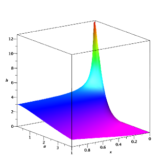
Figure 1: Plot of the three-dimensional surface of the hazard rate function when $b$=3 and $c$=0.5.

Here the CDF, equation (29), and the hazard rate function, equation (32), are reported in closed form in contrast to what was asserted by [12]. The mode of the GLD is at

$$Mode=\frac{-ab+ac+\sqrt{{a}^{2}{b}^{2}+2\,{a}^{2}bc+{a}^{2}{c}^{2}-4\,abc}}{2\,bc}\quad.$$ (33)

The $r$th moment about the origin for the GLD is

$$\mu^{\prime}_{r}=\frac{\Gamma\left(r+a\right)\left({b}^{-r}ca+{b}^{-r}cr+{b}^{-r+1}a\right)}{\left(c+b\right)\Gamma\left(a+1\right)}\quad,$$ (34)

and in particular the third moment is

$$\mu^{\prime}_{3}=\frac{\Gamma\left(3+a\right)\left(ab+ac+3\,c\right)}{\left(c+b\right)\Gamma\left(a+1\right){b}^{3}}\quad.$$ (35)

The three parameters $a$, $b$ and $c$ of the GLD can be obtained by numerically solving the following three non-linear equations

$$\mu =\bar{x}$$ (36a)

$$\sigma^{2} =s^{2}$$ (36b)

$$\mu^{\prime}_{3} =\bar{x}_{3}\quad.$$ (36c)

3.4 The new generalized Lindley distribution

The new generalized Lindley PDF with three parameters (NGLD) according to [13] is

$$f(x;a,b,c)=\frac{\left({c}^{a+1}{x}^{a-1}\Gamma\left(b\right)+{c}^{b}{x}^{b-1}\Gamma\left(a\right)\right){{\rm e}^{-cx}}}{\left(1+c\right)\Gamma\left(a\right)\Gamma\left(b\right)}\quad,$$ (37)

where $a$, $b$, $c$ and $x>0$. The CDF of the NGLD is

$$F(x;a,c,b)=\frac{NB}{\left(1+c\right)\Gamma\left(b+2\right)\Gamma\left(a+2\right)}\quad,$$ (38)

where

$$NB=\Gamma\left(b+2\right){x}^{a}{c}^{a+1}{{\rm e}^{-cx}}a+\Gamma\left(a+2\right){x}^{b}{c}^{b}{{\rm e}^{-cx}}b-\Gamma\left(b+2\right)c\Gamma\left(a+1,cx\right)a+$$

$$\Gamma\left(b+2\right){x}^{a}{c}^{a+1}{{\rm e}^{-cx}}+\Gamma\left(a+2\right){x}^{b}{c}^{b}{{\rm e}^{-cx}}-\Gamma\left(b+2\right)c\Gamma\left(a+1,cx\right)+\Gamma\left(b+2\right)\Gamma\left(a+2\right)c-$$

$$\Gamma\left(a+2\right)\Gamma\left(b+1,cx\right)b+\Gamma\left(b+2\right)\Gamma\left(a+2\right)-\Gamma\left(a+2\right)\Gamma\left(b+1,cx\right)$$ (39)

where $\Gamma(a,z)$ is the incomplete Gamma function, defined by

$$\mathop{\Gamma\/}\nolimits\!\left(a,z\right)=\int_{z}^{\infty}t^{a-1}e^{-t}dt\quad,$$ (40)

see [11]. The average value of the NGLD is

$$\mu(a,b,c)=\frac{ac+b}{c\left(1+c\right)}\quad,$$ (41)

and the variance of the NGLD is

$$\sigma^{2}(a,b,c)=\frac{{a}^{2}c-2\,abc+a{c}^{2}+{b}^{2}c+ac+bc+b}{{c}^{2}\left(1+c\right)^{2}}\quad.$$ (42)

The $r$th moment about the origin for the NGLD is

$$\mu^{\prime}_{r}=\frac{{c}^{-r+1}\Gamma\left(r+a\right)\Gamma\left(b\right)+{c}^{-r}\Gamma\left(r+b\right)\Gamma\left(a\right)}{\left(1+c\right)\Gamma\left(a\right)\Gamma\left(b\right)}\quad,$$ (43)

and the third moment is

$$\mu^{\prime}_{3}=\frac{\Gamma\left(3+a\right)\Gamma\left(b\right)c+\Gamma\left(3+b\right)\Gamma\left(a\right)}{{c}^{3}\left(1+c\right)\Gamma\left(a\right)\Gamma\left(b\right)}\quad.$$ (44)

The three parameters $a$, $b$ and $c$ of the NGLD are obtained by numerically solving the three non-linear equations (36a), (36b) and (36a).

3.5 The new weighted Lindley distribution

The new weighted Lindley PDF with two parameters (NWL) according to [14] is

$$f(x;b,c)=\frac{-{c}^{2}\left(1+b\right)^{2}\left(1+x\right)\left(-1+{{\rm e}^{-cbx}}\right){{\rm e}^{-cx}}}{b\left(cb+b+c+2\right)}\quad,$$ (45)

where $b$, $c$ and $x>0$. The CDF of the NWL is

$$F(x;c,b)=\frac{NC}{b\left(cb+b+c+2\right)}\quad,$$ (46)

where

$$NC=-{{\rm e}^{-cx}}{b}^{2}cx+{{\rm e}^{-c\left(1+b\right)x}}bcx-{{\rm e}^{-cx}}{b}^{2}c-2\,{{\rm e}^{-cx}}bcx+{{\rm e}^{-c\left(1+b\right)x}}bc$$

$$+{{\rm e}^{-c\left(1+b\right)x}}cx-{{\rm e}^{-cx}}{b}^{2}-2\,{{\rm e}^{-cx}}bc-{{\rm e}^{-cx}}cx+{b}^{2}c+{{\rm e}^{-c\left(1+b\right)x}}c-2\,{{\rm e}^{-cx}}b-{{\rm e}^{-cx}}c+{b}^{2}+cb$$

$$+{{\rm e}^{-c\left(1+b\right)x}}-{{\rm e}^{-cx}}+2\,b\quad.$$ (47)

The average value of the NWL is

$$\mu(a,b,c)=\frac{{b}^{2}c+2\,{b}^{2}+3\,cb+6\,b+2\,c+6}{\left(cb+b+c+2\right)c\left(1+b\right)}\quad,$$ (48)

and the variance of the NWL is

$$\sigma^{2}(a,b,c)=\frac{ND}{{c}^{2}\left(bc+b+c+2\right)^{2}\left(1+b\right)^{2}}\quad,$$ (49)

where

$$ND={b}^{4}{c}^{2}+4\,{b}^{4}c+4\,{b}^{3}{c}^{2}+2\,{b}^{4}+18\,{b}^{3}c+7\,{b}^{2}{c}^{2}+12\,{b}^{3}+32\,{b}^{2}c+6\,b{c}^{2}+24\,{b}^{2}$$

$$+30\,bc+2\,{c}^{2}+24\,b+12\,c+12\quad.$$ (50)

The $r$th moment about the origin for the NWL is

$$\mu^{\prime}_{r}=\frac{NE}{b\left(bc+b+c+2\right)}\quad,$$ (51)

where

$$NE=-\Big{(}{c}^{1-r}{b}^{1-r}({\frac{1+b}{b}})^{-r}+{b}^{-r}({\frac{1+b}{b}})^{-r}{c}^{-r}r-{c}^{-r}{b}^{2}r+{c}^{1-r}{b}^{-r}({\frac{1+b}{b}})^{-r}-{c}^{1-r}{b}^{2}$$

$$+{b}^{-r}({\frac{1+b}{b}})^{-r}{c}^{-r}-{c}^{-r}{b}^{2}-2\,{c}^{-r}br-2\,{c}^{1-r}b-2\,{c}^{-r}b-{c}^{-r}r-{c}^{1-r}-{c}^{-r}\Big{)}\Gamma(1+r)\quad.$$ (52)

The two parameters $b$ and $c$ of the NWL can be found by numerically solving the nonlinear system given by eqs (17a) and (17b).

4 The double truncated Lindley distribution

Let $X$ be a random variable defined in $[x_{l},x_{u}]$; the double truncated (DTL) version of the Lindley PDF with one parameter, $f_{t}(x;c,x_{l},x_{u})$, is

$$f_{t}(x;c,x_{l},x_{u})=\frac{{c}^{2}{{\rm e}^{-cx}}\left(x+1\right)}{{{\rm e}^{-c{\it x_{l}}}}c{\it x_{l}}-{{\rm e}^{-c{\it x_{u}}}}c{\it x_{u}}+{{\rm e}^{-c{\it x_{l}}}}c-{{\rm e}^{-c{\it x_{u}}}}c+{{\rm e}^{-c{\it x_{l}}}}-{{\rm e}^{-c{\it x_{u}}}}}\quad,$$ (53)

where the effect of the double truncation increases the parameters from one to three, see [15]. The double truncated Lindley distribution with scale, which has four parameters, was introduced in [10].

Its CDF, $F_{t}(x;b,c,x_{l},x_{u})$, is

$$F_{t}(x;b,c,x_{l},x_{u})=\frac{NF}{\left(\left(-1+\left(-{\it x_{u}}-1\right)c\right){{\rm e}^{c{\it x_{l}}}}+\left(1+\left({\it x_{l}}+1\right)c\right){{\rm e}^{c{\it x_{u}}}}\right)^{2}}\quad,$$ (54)

where

$$NF=-{{\rm e}^{c({\it x_{l}}+{\it x_{u}})}}\Big{(}-(1+({\it x_{l}}+1)c)^{2}{{\rm e}^{-c({\it x_{l}}-{\it x_{u}})}}-(1+(x+1)c)(1+({\it x_{u}}+1)c){{\rm e}^{c(-x+{\it x_{l}})}}$$

$$+\Big{(}(1+(x+1)c){{\rm e}^{c(-x+{\it x_{u}})}}+1+({\it x_{u}}+1)c\Big{)}(1+({\it x_{l}}+1)c)\Big{)}\quad.$$ (55)

The average value, $\mu_{t}(c,x_{l},x_{u})$, is

$$\mu_{t}(c,x_{l},x_{u})=\frac{\left(2+\left({{\it x_{u}}}^{2}+{\it x_{u}}\right){c}^{2}+\left(2\,{\it x_{u}}+1\right)c\right){{\rm e}^{c{\it x_{l}}}}-{{\rm e}^{c{\it x_{u}}}}\left(2+\left({{\it x_{l}}}^{2}+{\it x_{l}}\right){c}^{2}+\left(2\,{\it x_{l}}+1\right)c\right)}{-c\left(\left(-1+\left(-{\it x_{u}}-1\right)c\right){{\rm e}^{c{\it x_{l}}}}+{{\rm e}^{c{\it x_{u}}}}\left(1+\left({\it x_{l}}+1\right)c\right)\right)}\quad.$$ (56)

The $r$th moment about the origin for the DTL, $\mu^{\prime}_{r}(c,x_{l},x_{u})$, is

$$\mu^{\prime}_{r}(c,x_{l},x_{u})=\frac{NG}{\left(\left(1+\left({\it x_{l}}+1\right)c\right){{\rm e}^{-c{\it x_{l}}}}-\left(1+\left({\it x_{u}}+1\right)c\right){{\rm e}^{-c{\it x_{u}}}}\right)\left(r+1\right)}\quad,$$ (57)

where

$$NG=-{{\it x_{l}}}^{r/2}{{\rm e}^{-1/2c{\it x_{l}}}}\left({c}^{1-r/2}+{c}^{-r/2}\left(r+1\right)\right){{\sl M}_{r/2,r/2+1/2}\left(c{\it x_{l}}\right)}$$

$$+\left({c}^{1-r/2}+{c}^{-r/2}\left(r+1\right)\right){{\rm e}^{-1/2c{\it x_{u}}}}{{\it x_{u}}}^{r/2}{{\sl M}_{r/2,r/2+1/2}\left(c{\it x_{u}}\right)}$$

$$+c\left(r+1\right)\left({{\rm e}^{-c{\it x_{l}}}}{{\it x_{l}}}^{r+1}-{{\rm e}^{-c{\it x_{u}}}}{{\it x_{u}}}^{r+1}\right)\quad.$$ (58)

The three parameters which characterize the DTL can be found in the following way. Consider the sample of stellar masses ${\mathcal{X}}=x_{1},x_{2},\dots,x_{n}$ and let $x_{(1)}\geq x_{(2)}\geq\dots\geq x_{(n)}$ denote their order statistics, so that $x_{(1)}=\max(x_{1},x_{2},\dots,x_{n})$, $x_{(n)}=\min(x_{1},x_{2},\dots,x_{n})$. The first two parameters $x_{l}$ and $x_{u}$ are

$${x_{l}}=x_{(n)},\qquad{x_{u}}=x_{(1)}\quad.$$ (59)

The third parameter $c$ can be found by solving the following non-linear equation

$$\mu_{t}(c,x_{l},x_{u})=\bar{x}\quad.$$ (60)

5 Application to the IMF

We report the adopted statistics for four samples of stars which will be subject of fit, with the lognormal, the Lindley generalizations and the double truncated Lindley.

5.1 The involved statistics

The merit function $\chi^{2}$ is computed according to the formula

$$\chi^{2}=\sum_{i=1}^{n}\frac{(T_{i}-O_{i})^{2}}{T_{i}},$$ (61)

where $n$ is the number of bins, $T_{i}$ is the theoretical value, and $O_{i}$ is the experimental value represented by the frequencies. The theoretical frequency distribution is given by

$$T_{i}=N{\Delta x_{i}}p(x)\quad,$$ (62)

where $N$ is the number of elements of the sample, $\Delta x_{i}$ is the magnitude of the size interval, and $p(x)$ is the PDF under examination.

A reduced merit function $\chi_{red}^{2}$ is evaluated by

$$\chi_{red}^{2}=\chi^{2}/NF\quad,$$ (63)

where $NF=n-k$ is the number of degrees of freedom, $n$ is the number of bins, and $k$ is the number of parameters. The goodness of the fit can be expressed by the probability $Q$, see equation 15.2.12 in [16], which involves the degrees of freedom and $\chi^{2}$. According to [16] p. 658, the fit ‘may be acceptable’ if $Q>0.001$.

The Akaike information criterion (AIC), see [17], is defined by

$$AIC=2k-2ln(L)\quad,$$ (64)

where $L$ is the likelihood function and $k$ the number of free parameters in the model. We assume a Gaussian distribution for the errors and the likelihood function can be derived from the $\chi^{2}$ statistic $L\propto\exp(-\frac{\chi^{2}}{2})$ where $\chi^{2}$ has been computed by eqn. (61), see [18], [19]. Now the AIC becomes

$$AIC=2k+\chi^{2}\quad.$$ (65)

The Kolmogorov–Smirnov test (K–S), see [20, 21, 22], does not require binning the data. The K–S test, as implemented by the FORTRAN subroutine KSONE in [16], finds the maximum distance, $D$, between the theoretical and the astronomical CDF as well the significance level $P_{KS}$, see formulas 14.3.5 and 14.3.9 in [16]; if $P_{KS}\geq 0.1$, the goodness of the fit is believable.

5.2 The selected sample of stars

The first test is performed on NGC 2362 where the 271 stars have a range $1.47{M}_{\hbox{$\odot$}}\leavevmode\nobreak\ \geq\leavevmode\nobreak\ {M}\geq 0.11{M}_{\hbox{$\odot$}}$, see [23] and CDS catalog J/MNRAS/384/675/table1.

The second test is performed on the low-mass IMF in the young cluster NGC 6611, see [24] and CDS catalog J/MNRAS/392/1034. This massive cluster has an age of 2–3 Myr and contains masses from $1.5{M}_{\hbox{$\odot$}}\leavevmode\nobreak\ \geq\leavevmode\nobreak\ {M}\geq 0.02{M}_{\hbox{$\odot$}}$. Therefore the brown dwarfs (BD) region, $\approx\,0.2\,\mathcal{M}_{\hbox{$\odot$}}$ is covered.

The third test is performed on $\gamma$ Velorum cluster where the 237 stars have a range $1.31{M}_{\hbox{$\odot$}}\leavevmode\nobreak\ \geq\leavevmode\nobreak\ {M}\geq 0.15{M}_{\hbox{$\odot$}}$, see [25] and CDS catalog J/A+A/589/A70/table5.

The fourth test is performed on young cluster Berkeley 59 where the 420 stars have a range $2.24{M}_{\hbox{$\odot$}}\leavevmode\nobreak\ \geq\leavevmode\nobreak\ {M}\geq 0.15{M}_{\hbox{$\odot$}}$, see [26] and CDS catalog J/AJ/155/44/table3.

5.3 The lognormal distribution

Let $X$ be a random variable defined in $[0,\infty]$; the lognormal PDF, following [27] or formula (14.2) in [28], is

$$PDF(x;m,\sigma)=\frac{{{\rm e}^{-\,{\frac{1}{{2\,\sigma}^{2}}\left(\ln\left({\frac{x}{m}}\right)\right)^{2}}}}}{x\sigma\,\sqrt{2\,\pi}}\quad,$$ (66)

where $m$ is the median and $\sigma$ the shape parameter. The CDF is

$$CDF(x;m,\sigma)=\frac{1}{2}+\frac{1}{2}\,{\rm erf}\left(\frac{1}{2}\,{\frac{\sqrt{2}\left(-\ln\left(m\right)+\ln\left(x\right)\right)}{\sigma}}\right)\quad,$$ (67)

where erf$(x)$ is the error function, defined as

$$\mathop{\mathrm{erf}\/}\nolimits(x)=\frac{2}{\sqrt{\pi}}\int_{0}^{x}e^{-t^{2}}dt\quad,$$ (68)

see [11]. The average value or mean, $E(X)$, is

$$E(X;m,\sigma)=m{{\rm e}^{\frac{1}{2}\,{\sigma}^{2}}}\quad,$$ (69)

the variance, $Var(X)$, is

$$Var={{\rm e}^{{\sigma}^{2}}}\left({{\rm e}^{{\sigma}^{2}}}-1\right){m}^{2}\quad,$$ (70)

the second moment about the origin, $E^{2}(X)$, is

$$E(X^{2};m,\sigma)={m}^{2}{{\rm e}^{2\,{\sigma}^{2}}}\quad.$$ (71)

The statistics for the lognormal distribution for these four astronomical samples of stars are reported in Table 1.

Table 1: Numerical values of $\chi_{red}^{2}$, AIC, probability $Q$, $D$, the maximum distance between theoretical and observed CDF, and $P_{KS}$, significance level, in the K–S test of the lognormal distribution, see equation (66), for different mass distributions. The number of linear bins, $n$, is 20.

Cluster	parameters	AIC	$\chi_{red}^{2}$	$Q$	$D$	$P_{KS}$
NGC 2362	$\sigma$= 0.5, $\mu_{LN}=-0.55$	37.6	1.86	0.014	0.073	0.105
NGC 6611	$\sigma$= 1.03 , $\mu_{LN}=-1.26$	71.2	3.73	$1.31\,10^{-7}$	0.093	0.049
$\gamma$ Velorum	$\sigma$= 0.5 , $\mu_{LN}=-1.08$	55.1	2.84	$5.08\,10^{-5}$	0.092	0.033
Berkeley 59	$\sigma$= 0.49 , $\mu_{LN}=-0.92$	54.9	2.82	$5.49\,10^{-5}$	0.11	$6.46\,10^{-5}$

5.4 The generalizations of the Lindley distribution

The statistics for the Lindley distribution and its generalizations are reported in the following tables: Table 2 for the Lindley distribution with one parameter,

Table 2: Numerical values of $\chi_{red}^{2}$, AIC, probability $Q$, $D$, the maximum distance between theoretical and observed CDF, and $P_{KS}$, significance level, in the K–S test of the Lindley distribution with one parameter for different mass distributions. The number of linear bins, $n$, is 20.

Cluster	parameters	AIC	$\chi_{red}^{2}$	$Q$	$D$	$P_{KS}$
NGC 2362	$c=2.05$	95.57	5.03	3.36 $10^{-12}$	0.248	2.93 $10^{-15}$
NGC 6611	$c=2.94$	38.35	2.01	0.0053	0.077	0.161
$\gamma$ Velorum	$c=3.18$	90.59	4.66	$5.86\,10^{-11}$	0.322	$3.23\,10^{-22}$
Berkeley 59	$c=2.76$	149.6	7.76	$6.35\,10^{-22}$	0.323	$5.24\,10^{-39}$

Table 3 for the TPLD,

Table 3: Numerical values of $\chi_{red}^{2}$, AIC, probability $Q$, $D$, the maximum distance between theoretical and observed CDF, and $P_{KS}$, significance level, in the K–S test of the TPLD distribution with two parameters for different mass distributions. The number of linear bins, $n$, is 20.

Cluster	parameters	AIC	$\chi_{red}^{2}$	$Q$	$D$	$P_{KS}$
NGC 2362	$b=-0.099,c=4.2$	72.94	3.83	6.8 $10^{-8}$	0.129	1.76 $10^{-4}$
NGC 6611	$b=0.043,c=4.32$	59.11	3.06	1.23 $10^{-5}$	0.098	0.033
$\gamma$ Velorum	$b=-0.035,c=5.81$	67.74	3.54	$5\,10^{-7}$	0.14	$8\,10^{-5}$
Berkeley 59	$b=-0.032,c=4.75$	81.47	4.3	$2.35\,10^{-9}$	0.167	$8.62\,10^{-11}$

Table 4 for the PLD,

Table 4: Numerical values of $\chi_{red}^{2}$, AIC, probability $Q$, $D$, the maximum distance between theoretical and observed CDF, and $P_{KS}$, significance level, in the K–S test of the PLD distribution with two parameters for different mass distributions. The number of linear bins, $n$, is 20.

Cluster	parameters	AIC	$\chi_{red}^{2}$	$Q$	$D$	$P_{KS}$
NGC 2362	$b=2.66,c=2.28$	28.87	1.38	0.128	0.053	0.39
NGC 6611	$b=3.33,c=1.27$	53.53	2.75	8.88 $10^{-5}$	0.087	0.08
$\gamma$ Velorum	$b=4.64,c=1.64$	106.2	5.67	$8.59\,10^{-14}$	0.16	$2\,10^{-6}$
Berkeley 59	$b=3.48,c=1.54$	117.1	6.28	$8\,10^{-16}$	0.187	$2.37\,10^{-13}$

Table 5 for the GLD,

Table 5: Numerical values of $\chi_{red}^{2}$, AIC, probability $Q$, $D$, the maximum distance between theoretical and observed CDF, and $P_{KS}$, significance level, in the K–S test of the GLD distribution with three parameters for different mass distributions. The number of linear bins, $n$, is 20.

Cluster	parameters	AIC	$\chi_{red}^{2}$	$Q$	$D$	$P_{KS}$
NGC 2362	$a=4.80,b=8.38,c=12.01$	37.63	1.86	0.016	0.064	0.2
NGC 6611	$a=1.4,b=4.8,c=8$	64.34	3.43	1.96 $10^{-6}$	0.105	0.017
$\gamma$ Velorum	$a=2.53,b=6.5,c=0.00046$	83.08	4.53	$1.25\,10^{-9}$	0.15	$2.8\,10^{-5}$
Berkeley 59	$a=2.2,b=5.09,c=1$	100.6	5.56	$8.6\,10^{-13}$	0.179	$2.93\,10^{-12}$

Table 6 for the NGLD and

Table 6: Numerical values of $\chi_{red}^{2}$, AIC, probability $Q$, $D$, the maximum distance between theoretical and observed CDF, and $P_{KS}$, significance level, in the K–S test of the NGLD distribution with three parameters for different mass distributions. The number of linear bins, $n$, is 20.

Cluster	parameters	AIC	$\chi_{red}^{2}$	$Q$	$D$	$P_{KS}$
NGC 2362	$a=7.34,b=1.57,c=10.61$	48.64	2.5	5.4$10^{-4}$	0.075	0.086
NGC 6611	$a=3.14,b=-0.36,c=6.24$	111.08	6.18	1 $10^{-14}$	0.225	$9.22\,10^{-10}$
$\gamma$ Velorum	$a=4.19,b=11.51,c=12.2$	50	2.58	$3.4\,10^{-4}$	0.101	0.014
Berkeley 59	$a=5.73,b=19.57,c=14.46$	54.14	2.83	$8.1\,10^{-5}$	0.086	$3.2\,10^{-3}$

Table 7 for the NWL.

Table 7: Numerical values of $\chi_{red}^{2}$, AIC, probability $Q$, $D$, the maximum distance between theoretical and observed CDF, and $P_{KS}$, significance level, in the K–S test of the NWL distribution with two parameters for different mass distributions. The number of linear bins, $n$, is 20.

Cluster	parameters	AIC	$\chi_{red}^{2}$	$Q$	$D$	$P_{KS}$
NGC 2362	b=0.008, c= 3.889	59.72	3.09	9.85 $10^{-6}$	0.155	3.33 $10^{-6}$
NGC 6611	b=1.57 , c=3.77	68.46	3.58	3.81 $10^{-7}$	0.12	4.2  $10^{-3}$
$\gamma$ Velorum	b= 0.0027, c= 5.86	79	4.16	$6.2\,10^{-9}$	0.195	$1.86\,10^{-8}$
Berkeley 59	b=0.007, c= 5.015	95.13	5.06	$9\,10^{-12}$	0.19	$4.73\,10^{-15}$

The best fit for NGC 2362 is obtained with the PLD, see Figure 2.

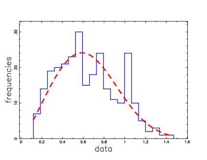
Figure 2: Empirical PDF of mass distribution for NGC 2362 cluster data (273 stars + BDs) when the number of bins, $n$, is 20 (steps with blue full line) with a superposition of the PLD (red dashed line). Theoretical parameters as in Table 4.

The best fit for NGC 6611 is obtained with the Lindley PDF with one parameter, see Figure 3.

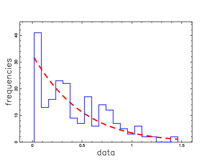
Figure 3: Empirical PDF of mass distribution for NGC 6611 cluster data when the number of bins, $n$, is 20 (steps with blue full line) with a superposition of the Lindley PDF with one parameter (red dashed line). Theoretical parameters as in Table 2.

The best fit for $\gamma$ Velorum is obtained with the lognormal PDF, see Figure 4.

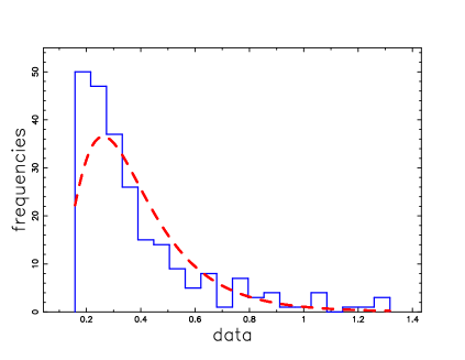
Figure 4: Empirical PDF of mass distribution for $\gamma$ Velorum cluster data when the number of bins, $n$, is 20 (steps with blue full line) with a superposition of the lognormal PDF (red dashed line). Theoretical parameters as in Table 1.

The best fit for the young cluster Berkeley 59 is obtained with the NGLD, see Figure 5.

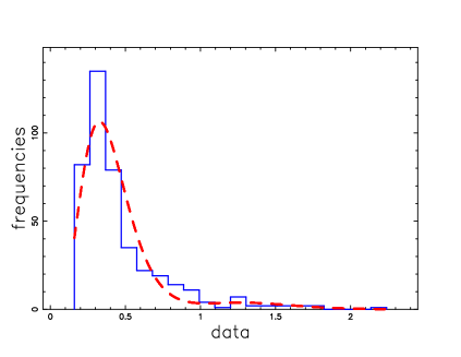
Figure 5: Empirical PDF of mass distribution for the young cluster Berkeley 59 when the number of bins, $n$, is 20 (steps with blue full line) with a superposition of the NGLD (red dashed line). Theoretical parameters as in Table 6.

5.5 The double truncated Lindley

The statistics for the DTL with three parameters are reported in Table 8.

Table 8: Numerical values of $\chi_{red}^{2}$, AIC, probability $Q$, $D$, the maximum distance between theoretical and observed CDF, and $P_{KS}$, significance level, in the K–S test of the DTL for different mass distributions. The number of linear bins, $n$, is 20.

Cluster	parameters	AIC	$\chi_{red}^{2}$	$Q$	$D$	$P_{KS}$
NGC 2362	$c=1.61$, $x_{l}=0.12$, $x_{u}=1.61$	156.7	8.86	1.75 $10^{-23}$	0.115	1.2 $10^{-3}$
NGC 6611	$c=2.71$, $x_{l}=0.019$, $x_{u}=1.46$	45.38	2.31	0.0015	0.061	0.395
$\gamma$ Velorum	$c=4.81$, $x_{l}=0.158$, $x_{u}=1.317$	45.89	2.34	$1.3\,10^{-3}$	0.064	0.269
Berkeley 59	$c=3.93$, $x_{l}=0.16$, $x_{u}=2.24$	78.57	4.26	$7.73\,10^{-9}$	0.134	$4.35\,10^{-7}$

Figure 6 reports the CDF of the DTL for NGC 6611 which is the the best fit of the various distributions here analysed for this cluster.

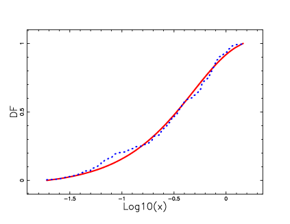
Figure 6: Empirical CDF of mass distribution for NGC 6611 cluster data (blue dotted line) with a superposition of the DTL CDF with one parameter (red line). Theoretical parameters as in Table 8.

6 Conclusions

In this paper we explored five generalizations of the Lindley distribution as well the double truncated Lindley distribution against the lognormal distribution. For each IMF of the four clusters here analysed, the distribution which realizes the best fit is reported in Table 9.

Table 9: Best fits: Name of the cluster, name of the distribution, $D$, the maximum distance between theoretical and observed CDF, and $P_{KS}$, significance level, in the K–S test.

Cluster	Best fit	$D$	$P_{KS}$
NGC 2362	PLD	0.053	0.39
NGC 6611	DTL	0.061	0.395
$\gamma$ Velorum	DTL	0.064	0.269
Berkeley 59	NWL	0.086	$3.2\,10^{-3}$

The above table allows to conclude that the Lindley family here suggested produces better fits than does the lognormal distribution. Figure 7 reports the CDF for NGC 6611 as well as four fitting curves.

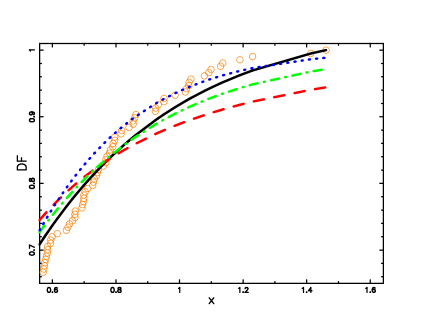
Figure 7: Part of the empirical CDF of mass distribution for NGC 6611 cluster data (orange circles) with a superposition of the DTL CDF with one parameter (black full line), the lognormal (red dashed line), the Lindley with one parameter (green dot-dash-dot-dash line) and the TPLD (blue dot line).

References

- [1] Lindley D V 1958 Fiducial distributions and Bayes’s theorem Journal of the Royal Statistical Society. Series B (Methodological) pp 102–107
- [2] Lindley D V 1965 Introduction to Probability and Statistics from a Bayesian Viewpoint (Cambridge: Cambridge University Press)
- [3] Shanker R and Mishra A 2013 A two-parameter Lindley distribution Statistics in Transition new series 1(14), 45
- [4] Ghitany M, Alqallaf F, Al-Mutairi D K and Husain H 2011 A two-parameter weighted Lindley distribution and its applications to survival data Mathematics and Computers in simulation 81(6), 1190
- [5] Mahmoudi E and Zakerzadeh H 2010 Generalized Poisson–Lindley distribution Communications in StatisticsTheory and Methods 39(10), 1785
- [6] Bakouch H S, Al-Zahrani B M, Al-Shomrani A A, Marchi V A and Louzada F 2012 An extended Lindley distribution Journal of the Korean Statistical Society 41(1), 75
- [7] Merovci F and Elbatal I 2013 Transmuted Lindley-geometric distribution and its applications arXiv preprint arXiv:1309.3774
- [8] Tomy L 2018 A retrospective study on Lindley distribution Biometrics and Biostatistics International Journal 7, 163
- [9] Shanker R and Mishra A 2014 A two-parameter Poisson-Lindley distribution International journal of Statistics and Systems 9(1), 79
- [10] Zaninetti L 2019 The Truncated Lindley Distribution with Applications in Astrophysics Galaxies 7(2), 61 (Preprint 1906.00739)
- [11] Olver F W J e, Lozier D W e, Boisvert R F e and Clark C W e 2010 NIST handbook of mathematical functions. (Cambridge: Cambridge University Press. )
- [12] Zakerzadeh H and Dolati A 2009 Generalized Lindley distribution Journal of Mathematical extension 3, 13
- [13] Ibrahim E, Merovci F and Elgarhy M 2013 A new generalized Lindley distribution Mathematical Theory and Modeling 3, 30
- [14] Asgharzadeh A, Bakouch H S, Nadarajah S, Sharafi F et al. 2016 A new weighted Lindley distribution with application Brazilian Journal of Probability and Statistics 30(1), 1
- [15] Singh S K, Singh U and Sharma V K 2014 The truncated Lindley distribution: Inference and application Journal of Statistics Applications & Probability 3(2), 219
- [16] Press W H, Teukolsky S A, Vetterling W T and Flannery B P 1992 Numerical Recipes in FORTRAN. The Art of Scientific Computing (Cambridge, UK: Cambridge University Press)
- [17] Akaike H 1974 A new look at the statistical model identification IEEE Transactions on Automatic Control 19, 716
- [18] Liddle A R 2004 How many cosmological parameters? MNRAS 351, L49
- [19] Godlowski W and Szydowski M 2005 Constraints on Dark Energy Models from Supernovae in M Turatto, S Benetti, L Zampieri and W Shea, eds, 1604-2004: Supernovae as Cosmological Lighthouses (Astronomical Society of the Pacific) vol 342 of Astronomical Society of the Pacific Conference Series pp 508–516
- [20] Kolmogoroff A 1941 Confidence limits for an unknown distribution function The Annals of Mathematical Statistics 12(4), 461 ISSN 00034851
- [21] Smirnov N 1948 Table for estimating the goodness of fit of empirical distributions The Annals of Mathematical Statistics 19(2), 279 ISSN 00034851
- [22] Massey Frank J J 1951 The kolmogorov-smirnov test for goodness of fit Journal of the American Statistical Association 46(253), 68
- [23] Irwin J, Hodgkin S, Aigrain S, Bouvier J, Hebb L, Irwin M and Moraux E 2008 The Monitor project: rotation of low-mass stars in NGC 2362 - testing the disc regulation paradigm at 5 Myr MNRAS 384, 675 (Preprint 0711.2398)
- [24] Oliveira J M, Jeffries R D and van Loon J T 2009 The low-mass initial mass function in the young cluster NGC 6611 MNRAS 392, 1034 (Preprint 0810.4444)
- [25] Prisinzano L, Damiani F and et al 2016 The Gaia-ESO Survey: membership and initial mass function of the Velorum cluster A&A 589 A70 (Preprint 1601.06513)
- [26] Panwar N, Pandey A K, Samal M R and et al 2018 Young Cluster Berkeley 59: Properties, Evolution, and Star Formation AJ 155(1) 44 (Preprint 1711.09353)
- [27] Evans M, Hastings N and Peacock B 2000 Statistical Distributions - third edition (New York: John Wiley & Sons Inc)
- [28] Johnson N L, Kotz S and Balakrishnan N 1994 Continuous univariate distributions. Vol. 1. 2nd ed. (New York: Wiley )