Null wave front as Ryu-Takayanagi surface

Abstract

The Ryu-Takayanagi formula provides the entanglement entropy of quantum field theory as an area of the minimal surface (Ryu-Takayangi surface) in a corresponding gravity theory. There are some attempts to understand the formula as a flow rather than as a surface. In this paper, we propose that null rays emitted from the AdS boundary can be regarded as such a flow. In particular, we show that in spherical symmetric static spacetimes with a negative cosmological constant, wave fronts of null geodesics from a point on the AdS boundary become extremal surfaces and therefore they can be regarded as the Ryu-Takayanagi surfaces. In addition, based on the viewpoint of flow, we propose a wave optical formula to calculate the holographic entanglement entropy.

I Introduction

It is well known that the entanglement entropy (EE) of conformal field theory (CFT) can calculate in a corresponding gravity theory by the Ryu-Takayanagi (RT) formula PhysRevLett.96.181602Ryu2006 ; Ryu:2006ef in AdS/CFT correspondence GUBSER1998105 ; Witten199801 . In general, although the EE of quantum field theory is not easy to calculate, the RT formula tells that the EE $S_{A}$ of a region $A$ in CFT can calculated as the area of the minimal bulk surface $\mathcal{M}_{A}$ homologous to $A$ (RT surface):

$$S_{A}=\frac{\mathrm{Area}\left(\mathcal{M}_{A}\right)}{4G_{N}},$$ (1)

where $G_{N}$ is the Newton constant of gravitation. This relation promotes informational theoretical analysis of AdS/CFT correspondence. By regarding the geometry of a bulk as a tensor network, it implements quantum error correcting code of boundary CFT Pastawski2015 or MERA Swingle2012 , subregion subregion correspondence which is proposed for reduced density matrix Czech_2012 .

From this point of view, it is better to regard the RT formula as a flow proposed by the paper Freedman:2016zud . The authors introduced “bit threads” which are equivalent concept to the RT surface geometrically. The bit threads are defined as a bounded divergenceless vector field $v^{\mu}$

$$\nabla_{\mu}v^{\mu}=0,\quad\left|v\right|\leq C,$$ (2)

and it maximizes its flux on a boundary area $A$. The property that the maximal total flux of $v^{\mu}$ through the area $A$ is equal to the area of the RT surface is proved by the max-flow min-cut theorem Freedman:2016zud . The bit threads give an intuitive picture that a vector field carrying information of the boundary propagates in the bulk, and the bulk region stores information of the boundary.

Although the concept of bit threads is inspirational, as mentioned by Freedman:2016zud , the RT surface has infinitely many equivalent bit threads. Moreover, it is non-trivial task to construct bit threads practically and to calculate the EE of CFT by it due to its dependence of global structure of spacetimes. Therefore, as one of the interpretations of the RT surface respecting the viewpoint of the flow, we propose an interpretation that the RT surfaces are wave fronts of null rays emitted from a point on the AdS boundary. In particular, we prove that in spherical symmetric static spacetimes, owing to its axisymmetry of the configuration, such wave fronts of null rays are extremal surfaces as long as they propagates in the vacuum region. As the RT surface is the extremal surface Fursaev:2006ih ; Lewkowycz2013 , thus the wave front can be considered as the RT surface. On the other hand, we can naturally understand null rays as bit threads. In this picture, we can calculate the EE of CFT by counting the number of such null rays. This method is also valid for wave optical calculation using the flux of a massless scalar field. The flux based calculation method suggests a picture that information prepared on the boundary side spreads to the bulk as null rays.

The structure of this paper is as follows. In Section 2, we demonstrate the correspondence between the RT surface and the wave front of the null rays in the BTZ spacetime. In Section 3, we state the detail of our proposal and show it in spherically symmetric static spacetimes with a negative cosmological constant. In Section 4, we introduce the flux formula to calculate the EE of CFT by counting the number of null rays. Finally, Section 5 is devoted to summary.

II Null wave front and RT surface

In this section, before going to discuss the general situation, we demonstrate that wave fronts of null rays are the RT surface in the BTZ spacetime.

II.1 Ryu-Takayanagi surface

We derive the equation of the RT surface in the BTZ spacetime PhysRevLett.69.1849Banados1992

$$ds^{2}=-\left(\frac{r^{2}}{\ell_{\text{AdS}}^{2}}-M\right)dt^{2}+\left(\frac{r^{2}}{\ell_{\text{AdS}}^{2}}-M\right)^{-1}dr^{2}+r^{2}d\theta^{2},\quad-\pi\leq\theta\leq\pi,$$ (3)

where $M$ is the mass of the black hole and $\ell_{\text{AdS}}$ is the AdS radius. We prepare a region (arc) $-\theta_{\ell}\leq\theta\leq\theta_{\ell}$ on the AdS boundary and consider a line anchored to the boundary of this region. The RT surface extremizes the following line area (length) on a constant time slice:

$$\mathrm{Area}\left[r(\cdot),\frac{dr}{d\theta}(\cdot)\right]=\int_{-\theta_{\ell}}^{\theta_{\ell}}d\theta\sqrt{\left(\frac{r^{2}}{\ell_{\text{AdS}}^{2}}-M\right)^{-1}\left(\frac{dr}{d\theta}\right)^{2}+r^{2}}.$$ (4)

The equation of the RT surface $r=r_{\text{RT}}(\theta)$ is the solution of the Euler-Lagrange equation obtained by variation of $\mathrm{Area}[r,dr/d\theta]$ with respect to $r$, and it is

$$r_{\text{RT}}(\theta)=\frac{\sqrt{M}\,r_{\mathrm{min}}\,\mathrm{sech}\left(\sqrt{M}\,\theta\right)}{\sqrt{M-r_{\mathrm{min}}^{2}/\ell_{\text{AdS}}^{2}\tanh^{2}\left(\sqrt{M}\,\theta\right)}},$$ (5)

where $r_{\mathrm{min}}:=r_{\text{RT}}(\theta=0)$ denotes the minimum of $r$ (see Fig. 1). Note that $\theta_{\ell}=\theta(r=\infty)=(1/\sqrt{M})\mathrm{arctanh}(\sqrt{M}\ell_{\text{AdS}}/r_{\text{min}})$.

Figure 1: The RT surface in the BTZ spacetime ($M=\ell_{\text{AdS}}=1$) with coordinates $(x,y)=(\rho\cos\theta,\rho\sin\theta)$, $\rho:=\ell_{\text{AdS}}\arctan\left(r/\ell_{\text{AdS}}\right)$. Each blue lines is parametrized by $r_{\mathrm{min}}=1.01,1.05,1.2,2.0,5.0$. For large interval $2\theta_{\ell}$ on the AdS boundary, dotted lines become minimal surfaces.

The entanglement entropy of CFT on the AdS boundary for an arc $|\theta|\leq\theta_{\ell}$ is obtained by substituting (5) into (4) :

$$\mathrm{Area}\left(\mathcal{M}_{\ell}\right)=2\ell_{\text{AdS}}\log\left(\frac{2\ell_{\text{AdS}}}{\epsilon\sqrt{M}}\sinh\left(\sqrt{M}\,\theta_{\ell}\right)\right)+O(\epsilon),$$ (6)

where the cutoff is introduced by $\epsilon:=\ell_{\text{AdS}}^{2}/r~{}(r\rightarrow\infty)$. Now let us consider CFT with inverse temperature $\beta$ on $\mathrm{S}^{1}$. The circumference of the circle is assumed to be $C$ and we prepare an arc $|\theta|\leq\theta_{\ell}$ with the arc length $\ell=C\theta_{\ell}/\pi$ on it. Then it is possible to write down (6) using only CFT quantities. By dividing Eq. (6) with $4G_{N}$, using the Brown-Henneaux formula $c=3\ell_{\text{AdS}}/(2G_{N})$ Brown1986 and AdS/CFT dictionary $\beta/C=1/\sqrt{M}$, we obtain the correct EE formula of thermal state of CFT on $\mathrm{S}^{1}$  Calabrese:2004eu ; Calabrese:2009qy after rescaling the cutoff $\epsilon$:

$$S_{A}=\frac{c}{3}\log\left(\frac{\beta}{\pi\epsilon}\sinh\left(\frac{\pi\ell}{\beta}\right)\right).$$ (7)

II.2 Null rays and wave front

We consider null rays emitted from a point on the AdS boundary and their wave fronts. Our purpose is to find out the relation between wave fronts of null rays and the RT surface. We consider null rays in the spherically symmetric static spacetime

$$ds^{2}=-f(r)dt^{2}+\frac{dr^{2}}{f(r)}+r^{2}d\Omega_{d-1}^{2},$$ (8)

where $d$ denotes spatial dimension and $d\Omega_{d-1}^{2}$ is the line element of the unit sphere $\mathrm{S}^{d-1}$. We introduce coordinates on $\mathrm{S}^{d-1}$ as

$$\begin{bmatrix}x_{1}\\ x_{2}\\ x_{3}\\ \vdots\\ x_{d-2}\\ x_{d-1}\end{bmatrix}=\begin{bmatrix}\cos\psi_{1}\hfill\\ \sin\psi_{1}\cos\psi_{2}\hfill\\ \sin\psi_{1}\sin\psi_{2}\hfill\\ \vdots\\ \sin\psi_{1}\sin\psi_{2}\cdots\sin\psi_{d-2}\cos\psi_{d-1}\\ \sin\psi_{1}\sin\psi_{2}\cdots\sin\psi_{d-2}\sin\psi_{d-1}\end{bmatrix}$$ (9)

with $0\leq\psi_{1},\cdots\psi_{d-2}\leq\pi,~{}0\leq\psi_{d-1}\leq 2\pi$. The line element on $\mathrm{S}^{d-1}$ is

$$d\Omega_{d-1}^{2}=d\psi_{1}^{2}+\sin^{2}\psi_{1}(d\psi_{2}^{2}+\sin^{2}\psi_{2}(d\psi_{3}^{2}+\cdots\cdots)).$$ (10)

As is well known, in static spherically symmetric spacetimes, trajectories of null geodesics stay on a spatial two dimensional plane. Thus we can fix coordinate values of $\psi_{2},\cdots\psi_{d-1}$ and assume the following (2+1)-dimensional metric to investigate wave fronts of null rays emitted from a point:

$$ds^{2}=-f(r)dt^{2}+\frac{dr^{2}}{f(r)}+r^{2}d\theta^{2},\quad\theta:=\psi_{1}.$$ (11)

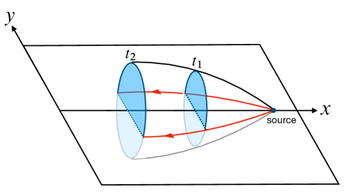
Figure 2: Axisymmetric configuration of congruence of null rays. Coordinates on two dimensional plane are introduced by $(x,y)=(r\cos\theta,r\sin\theta)$. Wave fronts at fixed $t$ are symmetric with respect to rotation about $x$-axis. Projection of null rays on the $(x,y)$-plane are shown as red lines.

In this metric with coordinates $x^{\mu}=(t,r,\theta)$, a wave front of null rays emitted from a point source is defined as a $t=$ constant section of null congruences, which forms a $(d-1)$-dimensional surface. Due to the axial symmetry of the configuration, a wave front of null rays is represented as a curve in $(r,\theta)$ space in the present situation. The tangent vector of a null ray is

$$k^{\mu}=(k^{t},k^{r},k^{\theta})=\left(\frac{dt}{d\lambda},\frac{dr}{d\lambda},\frac{d\theta}{d\lambda}\right),\quad-f\left(\frac{dt}{d\lambda}\right)^{2}+\frac{1}{f}\left(\frac{dr}{d\lambda}\right)^{2}+r^{2}\left(\frac{d\theta}{d\lambda}\right)^{2}=0,$$ (12)

where $\lambda$ is the affine parameter. This spacetime has two Killing vectors related to translation of $t$ and $\theta$ directions and there exist two conserved charges $\omega:=f(r)\dfrac{dt}{d\lambda},\ p_{\theta}:=r^{2}\dfrac{d\theta}{d\lambda}$. Combining with Eq. (12), we obtain a trajectory of a null ray as

$$\theta(r) =\theta_{0}\pm\int_{r_{0}}^{r}\frac{b}{r^{\prime 2}}\left(1-f(r^{\prime})\frac{b^{2}}{r^{\prime 2}}\right)^{-\frac{1}{2}}dr^{\prime},$$ (13)

$$t(r) =t_{0}\pm\int_{r_{0}}^{r}\frac{1}{f(r^{\prime})}\left(1-f(r^{\prime})\frac{b^{2}}{r^{\prime 2}}\right)^{-\frac{1}{2}}dr^{\prime},$$ (14)

$$\lambda(r) =\lambda_{0}\pm\frac{1}{\omega}\int_{r_{0}}^{r}\left(1-f(r^{\prime})\frac{b^{2}}{r^{\prime 2}}\right)^{-\frac{1}{2}}dr^{\prime},$$ (15)

where $(t_{0},\theta_{0},\lambda_{0})=(t(r_{0}),\theta(r_{0}),\lambda(r_{0}))$ and the impact parameter $b:=p_{\theta}/\omega$ is introduced. The sign $\pm$ in front of the integral corresponds to the sign of $dr/d\lambda$.

For the $(2+1)$-dimensional BTZ spacetime (3), we can demonstrate explicitly that wave fronts of null rays are the RT surfaces. We obtain equations of null geodesic from (13) and (14) with $(t_{0},r_{0},\theta_{0})=(0,\infty,0)$:

$$\theta(r) =\frac{1}{\sqrt{M}}\log\left[\frac{\sqrt{r^{2}-b^{2}\left(r^{2}/\ell_{\text{AdS}}^{2}-M\right)}+b\sqrt{M}}{r\sqrt{1-b^{2}/\ell_{\text{AdS}}^{2}}}\right],$$ (16)

$$t(\theta) =\frac{\ell_{\text{AdS}}}{\sqrt{M}}\mathrm{arctanh}\left(\frac{\ell_{\text{AdS}}}{b}\tanh\left(\sqrt{M}\,\theta\right)\right).$$ (17)

It is easy to derive a trajectory of a null ray $r=r_{\text{NG}}(\theta,b)$ with an impact parameter $b$ from (16). On the other hand, the equation of a wave front $r=r_{\text{WF}}(\theta,t)$ at a fixed $t$ is derived by eliminating the parameter $b$ from (16) and (17). After all,

$$r_{\text{NG}}(\theta,b) =\frac{\sqrt{M}\,b}{\sqrt{1-b^{2}/\ell_{\text{AdS}}^{2}}}\,\mathrm{csch}\left(\sqrt{M}\,\theta\right),$$ (18)

$$r_{\text{WF}}(\theta,t) =\frac{\sqrt{M}\ell_{\text{AdS}}\,\mathrm{coth}\left(\sqrt{M}\,t/\ell_{\text{AdS}}\right)\mathrm{sech}\left(\sqrt{M}\,\theta\right)}{\sqrt{1-\mathrm{coth}^{2}\left(\sqrt{M}\,t/\ell_{\text{AdS}}\right)\mathrm{tanh}^{2}\left(\sqrt{M}\,\theta\right)}}.$$ (19)

For the special case $M=-1$, the spacetime reduces to the pure AdS. Figure 3 and Figure 4 show null rays and their wave fronts in the pure AdS spacetime and the BTZ black hole spacetime, respectively.

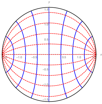
Figure 3: Null rays (dotted red lines) and wave fronts (blue lines) in the pure AdS₂₊₁ spacetime $(M=-1,\ell_{\text{AdS}}=1)$.

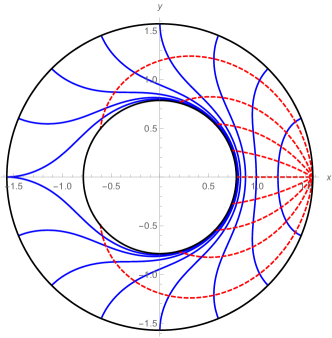
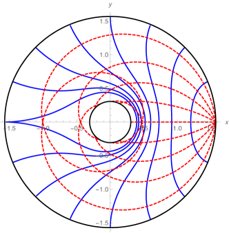
Figure 4: Null rays (dotted red lines) emitted from $(r,\theta)=(\infty,0)$ and their wave fronts (blue lines) in the BTZ spacetime (left panel: $M=\ell_{\text{AdS}}=1$, right panel: $M=0.1,\ell_{\text{AdS}}=1$).

Note that Eq. (19) of the wave front is the same as Eq. (5) of the RT surface by identifying $r_{\mathrm{min}}=\sqrt{M}\ell_{\text{AdS}}\coth\left(\sqrt{M}t/\ell_{\text{AdS}}\right)$, which represents the elapsed time of a null ray traveling from $r=\infty$ to $r=r_{\mathrm{min}}$. Indeed this quantity is obtained by taking $b=0$ in the equation of the null ray (14):

$$t=\int_{\infty}^{r_{\mathrm{min}}}\frac{dr}{r^{2}/\ell_{\text{AdS}}^{2}-M}=\frac{\ell_{\text{AdS}}}{\sqrt{M}}\!\ \mathrm{arctanh}\left(\frac{\sqrt{M}\ell_{\text{AdS}}}{r_{\mathrm{min}}}\right).$$ (20)

Therefore, we have confirmed that wave fronts of null rays emitted from the AdS boundary coincide with the RT surfaces in the BTZ spacetime. For sufficient elapse of time after emission of null rays, self-intersection of the wave front occurs and identification of the wave front as the RT surface becomes ambiguous.

III Null wave front and extremal surface

In this section, based on the observation in the previous section for the BTZ spacetime, we show the following proposition for spherically symmetric static spacetimes with a cosmological constant (no matter fields).

Proposition  Wave fronts of null rays emitted from a point are extremal surfaces when the affine parameter of null rays goes to infinity.

Corollary  For spacetimes with a negative cosmological constant, wave fronts of null rays emitted from a point on the AdS boundary are extremal surfaces.

We adopt the metric (11) with coordinates $x^{\mu}=(t,r,\theta,\cdots)$. Let $\xi^{\mu}=(\partial_{t})^{\mu}$ be the time-like Killing vector, $k^{\mu}=dx^{\mu}/d\lambda$ be the tangent vector of null geodesics. We introduce the projection tensor $P^{\mu\nu}=g^{\mu\nu}-\xi^{-2}\xi^{\mu}\xi^{\nu}=\mathrm{diag}(0,f,1/r^{2},\cdots)$ onto a constant time slice. We denote the tangent vector of null geodesics projected onto the hypersurface as $\tilde{k}^{i}=P^{i}{}_{j}\,k^{j}=(k^{r},k^{\theta},0,\cdots)$. The conserved quantity associated with the Killing vector is $\omega=-\xi^{\mu}k_{\mu}=fk^{t}$ and the norm of the spatial vector $\tilde{k}^{i}$ is $\tilde{k}^{i}\tilde{k}_{i}=\omega^{2}/f$.

We prove the proposition by using the fact that the extremal surface is a surface with zero mean curvature. The mean curvature $H$ of a wave front of null rays on a constant time slice is defined by

$$H:=D_{i}\tilde{n}^{i},\quad\tilde{n}^{i}=\frac{\tilde{k}^{i}}{\tilde{k}}=\frac{f^{1/2}}{\omega}(k^{r},k^{\theta},0,\cdots),$$ (21)

where $\tilde{n}^{i}$ is the unit normal vector of the wave front and $D_{i}=P_{i}{}^{j}\nabla_{j}=(\nabla_{r},\nabla_{\theta},\cdots)$ is the covariant derivative on a constant time slice. Then,

$$H =D_{i}\left(\frac{f^{1/2}}{\omega}k^{i}\right)=\frac{1}{f^{-1/2}\sqrt{h}}\partial_{i}\left(\frac{f^{1/2}}{\omega}f^{-1/2}\sqrt{h}\,k^{i}\right)$$

$$=\frac{f^{1/2}}{\omega\sqrt{h}}\left(\partial_{r}(\sqrt{h}\,k^{r})+\partial_{\theta}(\sqrt{h}\,k^{\theta})\right),$$ (22)

where $\sqrt{h}=r^{d-1}$ comes from determinant of the metric on $\mathrm{S}^{d-1}$. On the other hand, the expansion of a null congruence is

$$\Theta =\nabla_{\mu}k^{\mu}=\frac{1}{\sqrt{h}}\partial_{\mu}(\sqrt{h}\,k^{\mu})$$

$$=\frac{1}{\sqrt{h}}\left(\partial_{r}(\sqrt{h}\,k^{r})+\partial_{\theta}(\sqrt{h}\,k^{\theta})\right).$$ (23)

Therefore $H=(f^{1/2}/\omega)\Theta$ and the mean curvature $H$ of a wave front is proportional to the expansion of the null geodesic congruence. The expansion $\Theta$ along a null geodesic obeys the Raychaudhuri equation

$$\frac{d\Theta}{d\lambda}=-\frac{\Theta^{2}}{d-1}-R_{\mu\nu}k^{\mu}k^{\nu}.$$ (24)

In the present case, as the congruence of null geodesics has axial symmetry, the shear and the rotation of the congruence do not appear in this equation. For vacuum spacetimes with a cosmological constant, the term with the Ricci curvature disappears. Then the solution of Eq. (24) is $\Theta(\lambda)=(d-1)/(\lambda-\lambda_{0})$ where $\lambda_{0}$ is the affine parameter at the source. Thus the expansion goes to zero as the affine parameter goes to infinity, and the mean curvature of the wave front is zero and is the extremal surface. Therefore the proposition is proved. As an example of this proposition, let us consider a wave front in the Minkowski spacetime. A spherical wave front emitted from a point source placed at the spatial infinity becomes plane wave, which is zero mean curvature surface in the Minkowski spacetime. However, in this case, the coordinate time (14) becomes infinite when a wave front of null rays arrives at an observer.

Asymptotically AdS spacetimes are peculiar because they have the timelike boundary. We consider the pure AdS spacetime of which metric function is given by $f(r)=1+r^{2}/\ell_{\text{AdS}}^{2}$. As $f\approx r^{2}/\ell_{\text{AdS}}^{2}$ in the vicinity of the AdS boundary, the affine parameter of null rays (15) from the AdS boundary $r_{0}=\ell_{\text{AdS}}^{2}/\epsilon,\epsilon\rightarrow 0$ diverges as

$$\lambda(r)\approx\frac{1}{\omega}\int_{r}^{\ell_{\text{AdS}}^{2}/\epsilon}\left(1-\frac{b^{2}}{\ell_{\text{AdS}}^{2}}\right)^{-1/2}dr=\frac{\ell_{\text{AdS}}^{2}/\epsilon-r}{\omega\sqrt{1-b^{2}/\ell_{\text{AdS}}^{2}}}\to\infty.$$ (25)

On the other hand, the coordinate time (14) converges as

$$t(r)\approx\int_{r}^{\ell_{\text{AdS}}^{2}/\epsilon}dr\frac{\ell_{\text{AdS}}^{2}}{r^{2}}\left(1-\frac{b^{2}}{\ell_{\text{AdS}}^{2}}\right)^{-1/2}=\frac{\ell_{\text{AdS}}^{2}}{\sqrt{1-b^{2}/\ell_{\text{AdS}}^{2}}}\,\frac{1}{r}.$$ (26)

This property also holds for general asymptotically AdS spacetimes because they have the same metric in the vicinity of the AdS boundary as the pure AdS spacetime. After all, we conclude that for static spherical symmetric asymptotically AdS spacetimes, wave fronts of a null geodesic congruence emitted from a point source on the AdS boundary are extremal surfaces.

IV Flux formula

Based on the idea presented in the previous section, we can understand null rays as a natural flow characterizing the EE of the dual CFT. Hence a congruence of null rays is one of the bit threads described in Section I. This makes us conceive a picture that null rays propagate in the bulk with information of the AdS boundary. This picture suggests that the EE can be calculable by counting the number of null rays. In this section, we reformulate the RT formula in terms of the wave optics. Concepts of wave fronts and the flux of null rays are naturally derived as the eikonal limit of wave optics. As an application of wave optics to black hole spacetimes, papers Kanai2013 ; Nambu2016 ; Hashimoto2020 investigate image formation of the photon sphere of black holes. In this paper, we focus on the structure of wave fronts of a massless scalar field. For the monochromatic massless scalar field with time dependence $\propto e^{-i\omega t}$, we present wave patterns in Fig. 5 and Fig. 6 (see detail in Appendix). They show wave fronts from a point wave source on the AdS bounary (see Fig. 3 and Fig. 4 for corresponding wave fronts in the geometrical optics).

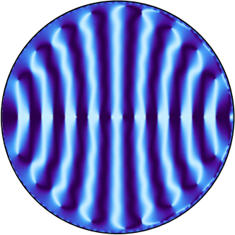
Figure 5: Wave pattern of the monochromatic massless scalar field with $\omega=20$ in the AdS spacetime. Real part of $\phi/|\phi|$ is shown.

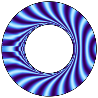
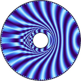
Figure 6: Wave pattern of the massless scalar field with $\omega=20$ (Re $\phi/|\phi|$) in the BTZ spacetime with $M=1$ (left panel) and $M=0.1$ (right panel).

For the massless scalar field $\phi(x^{\mu})$ obeying the Klein-Gordon equation $\square\phi=(\sqrt{-g})^{-1}\partial_{\mu}(\sqrt{-g}g^{\mu\nu}\partial_{\nu}\phi)=0$, the WKB form of the wave function is

$$\phi(x^{\mu})=a(x^{\mu})\exp\left[iS(x^{\mu})\right],$$ (27)

where $a$ and $S$ are real functions. In the eikonal limit, they obey

$$g^{\mu\nu}\nabla_{\mu}S\nabla_{\nu}S=0,$$ (28)

$$\nabla_{\mu}(a^{2}\nabla^{\mu}S)=0.$$ (29)

The equation (28) is the Hamilton-Jacobi (HJ) equation and Eq. (29) represents conservation of the Klein-Gordon current $J^{\mu}=(1/2i)(\phi^{*}\partial^{\mu}\phi-\phi\partial^{\mu}\phi^{*})$. In terms of the wave vector $k_{\mu}=\partial_{\mu}S$, which defines the tangent of null rays,

$$g_{\mu\nu}k^{\mu}k^{\nu}=0,\quad\nabla_{\mu}(a^{2}k^{\mu})=0.$$ (30)

For the stationary case, the phase function $S$ can be written as $S=-\omega t+W(r,\theta)$,

$$\tilde{k}^{i}=(k^{r},k^{\theta},0,\cdots)=\left(fW_{r},\frac{1}{r^{2}}W_{\theta},0,\cdots\right),\quad\tilde{k}^{i}\tilde{k}_{i}=\frac{\omega^{2}}{f},$$ (31)

$$f^{-1/2}D_{i}\left(a^{2}f^{1/2}\tilde{k}^{i}\right)=0.$$ (32)

Here, $\tilde{k}^{i}$ represents the tangent vector of null rays projected on a constant time slice. We can write the solution of (29) as

$$a(\lambda,\chi)=a(\lambda_{0},\chi)\exp\left(-\frac{1}{2}\int_{\lambda_{0}}^{\lambda}d\lambda\,\Theta(\lambda)\right),\quad\Theta=\nabla_{\mu}k^{\mu},$$ (33)

where the integral is along a null ray (with respect to the affine parameter $\lambda$) and $\chi$ denotes a coordinate distinguishing different geodesics. As the expansion of null congruence from the AdS boundary is zero, the amplitude $a(\lambda,\chi)$ is conserved along a null ray and independent of $\lambda$. Furthermore, for a point source isotropically emitting null rays, $a$ is independent of $\chi$ and can assume to be constant. Thus (32) implies

$$D_{i}\tilde{n}^{i}=0,\quad\tilde{n}^{i}=\frac{f^{1/2}}{\omega}\tilde{k}^{i},\quad\tilde{n}^{i}\tilde{n}_{i}=1,$$ (34)

and $\tilde{n}^{i}$ is divergenceless normalized vector field. The wave front is the surface with the unit normal $\tilde{n}^{i}$, and is the extremal surface. The number of null rays passing through the wave front $\mathcal{E}_{A}$, which is the extremal surface homologous to the region $A$ on the AdS boundary, is

$$\mathrm{Area}(\mathcal{E}_{A})=\int_{\mathcal{E}_{A}}\tilde{n}^{i}d\Sigma_{i},\quad d\Sigma_{i}=\tilde{n}_{i}\sqrt{h}\,d^{d-1}\sigma,$$ (35)

where $\sqrt{h}$ denotes determinant of the induced metric on $\mathcal{E}_{A}$. Now let us consider the setup shown as Fig. 7. We prepare a screen $A(\epsilon)$ which is $r=$constant surface in the bulk. For the regularization, the screen is placed at $r=\ell_{\text{AdS}}^{2}/\epsilon$ near the AdS boundary.

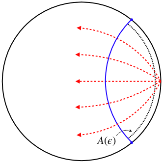
Figure 7: Null rays (red dotted lines) emitted from a point on the AdS boundary pass through the screen $A(\epsilon)$ placed at $r=\ell_{\text{AdS}}^{2}/\epsilon$ (dotted line). As the null rays are orthogonal to the wave front (blue line), the number of null rays is proportional to the area of the RT surface.

Because $\tilde{n}^{i}$ is divergence free vector field, Eq. (35) equals to

$$\mathrm{Area}(\mathcal{E}_{A})=\int_{A(\epsilon)}\tilde{n}^{i}d\Sigma_{i}=\frac{1}{\omega}\int_{A(\epsilon)}J^{i}d\Sigma_{i}.$$ (36)

This is a formula for area of the RT surface in terms of flux integration of null rays on the screen $A(\epsilon)$. As the Klein-Gordon current $J^{i}/\omega=f^{1/2}\tilde{k}^{i}/\omega$ represents the number density of null rays, we can regard the Klein-Gordon current as a representation of the amount of information propagating in the bluk from the AdS bounary.

As a demonstration, we evaluate the right hand side of this relation for the BTZ spacetime. By fixing the radial coordinate as $r=\ell_{\text{AdS}}^{2}/\epsilon$ in Eq. (18), the impact parameter $b$ on the screen is

$$b=\frac{\ell_{\text{AdS}}^{2}\sinh\left(\sqrt{M}\,\theta\right)}{\sqrt{\epsilon^{2}M+\ell_{\text{AdS}}^{2}\sinh^{2}\left(\sqrt{M}\,\theta\right)}}.$$ (37)

From Eq. (12), the radial component of the tangent vector of the null ray is

$$\frac{\tilde{k}^{r}}{\omega}=\left(1-f\,\frac{b^{2}}{r^{2}}\right)^{1/2}=\sqrt{1-\left(\frac{r^{2}}{\ell_{\text{AdS}}^{2}}-M\right)\frac{b^{2}}{r^{2}}},$$ (38)

and on the screen,

$$\left.\frac{\tilde{k}^{r}}{\omega}\right|_{A(\epsilon)}=\frac{\sqrt{M}\cosh\left(\sqrt{M}\,\theta\right)}{\sqrt{M+(\ell_{\text{AdS}}^{2}/\epsilon^{2})\sinh^{2}\left(\sqrt{M}\,\theta\right)}}.$$ (39)

The area element on the screen is

$$\left.d\Sigma_{r}\right|_{A(\epsilon)}=\left.r\,n_{r}\,d\theta\right|_{A(\epsilon)}=rf^{-1/2}d\theta,$$ (40)

where $n_{r}$ is the radial component of the unit normal to the screen. Thus

$$f^{1/2}\frac{\tilde{k}^{r}}{\omega}\left.d\Sigma_{r}\right|_{A(\epsilon)}=r\left(1-f\,\frac{b^{2}}{r^{2}}\right)^{1/2}\!\!\!\!d\theta=\frac{\sqrt{M}\ell_{\text{AdS}}\cosh(\sqrt{M}\theta)d\theta}{\sqrt{\sinh^{2}(\sqrt{M}\theta)+M\epsilon^{2}/\ell_{\text{AdS}}^{2}}}.$$ (41)

Therefore, (36) become

$$\int_{-\theta_{\ell}}^{\theta_{\ell}}\frac{f^{1/2}\tilde{k}^{i}d\Sigma_{i}}{\omega} =\int_{-\theta_{\ell}}^{\theta_{\ell}}d\theta\frac{\sqrt{M}\ell_{\text{AdS}}\cosh\left(\sqrt{M}\,\theta\right)}{\sqrt{M\epsilon^{2}/\ell_{\text{AdS}}^{2}+\sinh^{2}\left(\sqrt{M}\,\theta\right)}}$$

$$=\ell_{\text{AdS}}\log\left[\frac{\sqrt{\sinh^{2}(\sqrt{M}\,\theta_{\ell})+M\epsilon^{2}/\ell_{\text{AdS}}^{2}}+\sinh(\sqrt{M}\theta_{\ell})}{\sqrt{\sinh^{2}(\sqrt{M}\,\theta_{\ell})+M\epsilon^{2}/\ell_{\text{AdS}}^{2}}-\sinh(\sqrt{M}\theta_{\ell})}\right]$$

$$=2\ell_{\text{AdS}}\log\left[\frac{\ell_{\text{AdS}}}{(\epsilon/2)\sqrt{M}}\sinh\left(\sqrt{M}\,\theta_{\ell}\right)\right]+O(\epsilon),$$ (42)

and reproduces the “area” of the RT surface (6). Dividing by $4G_{N}$, this result correctly reproduces the EE of CFT (7). Therefore, we can regard such a null geodesic congruence as one realization of the bit threads.

V Summary

In this paper, we show that wave fronts of null rays emitted from a point on the AdS boundary are extremal surfaces in static spherical symmetric spacetimes. Thus the RT surface can be understood as a wave front, and null rays naturally define a flow characterizing the amount of the EE of CFT. Hence such a flow can be regarded as the bit threads.

As we assumed a point source on the AdS boundary, the shape of a region on the AdS boundary (entangling surface) becomes spherical because the boundary of the region is a wave front on the AdS boundary. However, by superposing point sources, it is possible to construct an extremal surface homologous to a region with arbitrary shapes on the AdS boundary by considering the envelope of wave fronts from each point sources. Thus the method presented in this paper may be applicable to the plateaux problem Hubeny2013 ; Freivogel2015 with non-trivial shapes of an entangling surface and to further understanding of property of the holographic EE.

Appendix A Massless scalar field in AdS spacetimes

We consider the solution of the Klein-Gordon equation $\square\phi=0$ in the AdS spacetime with the metric (8). Assuming the axially symmetric and stationary configuration of the scalar field $\phi=e^{-i\omega t}\tilde{\phi}(r,\theta)$, $\tilde{\phi}$ obeys the following Helmholtz type equation

$$\frac{\partial^{2}\tilde{\phi}}{\partial r^{2}}+\left(\frac{d-1}{r}+\frac{f^{\prime}}{f}\right)\frac{\partial\tilde{\phi}}{\partial r}+\frac{\omega^{2}}{f^{2}}\tilde{\phi}+\frac{1}{fr^{2}\sin^{d-2}\theta}\frac{\partial}{\partial\theta}\left(\sin^{d-2}\theta\,\frac{\partial\tilde{\phi}}{\partial\theta}\right)=0.$$ (43)

Assuming $\tilde{\phi}=R(r)\Phi(\theta)$,

$$R^{\prime\prime}+\left(\frac{d-1}{r}+\frac{f^{\prime}}{f}\right)R^{\prime}+\left(\frac{\omega^{2}}{f^{2}}-\frac{m(m+d-2)}{fr^{2}}\right)R=0,$$ (44)

$$\Phi_{\theta\theta}+(d-2)\cot\theta\,\Phi_{\theta}+m(m+d-2)\Phi=0,$$ (45)

and $\Phi=C_{m}^{d/2-1}(\cos\theta)$ (Gegenbauer polymonial). For $d=2$, $\Phi=e^{im\theta},~{}m\in\mathbb{Z}$ and for $d=3$, $\Phi=P_{m}(\cos\theta),~{}m\in\mathbb{Z}_{+}$. We consider $d=2$ case. For the normalized radial function $\lim_{r\rightarrow\infty}R_{m}(r)=1$, the solution of the Klein-Gordon equation with a point source at the AdS boundary is represented as

$$\phi(r,\theta)=\sum_{m=-\infty}^{m=\infty}e^{im\theta}R_{m}(r),$$ (46)

and this wave function gives $\lim_{r\rightarrow\infty}\phi\propto\delta(\theta)$ and satisfies the boundary condition with a point wave source at the AdS boundary. For the BTZ spacetime, the solution satisfying the ingoing boundary condition at the black hole horizon is given by

$$R_{m}=\frac{\Gamma(a)\Gamma(b)}{\Gamma(c)}\xi^{-i\frac{\ell_{\text{AdS}}\omega}{2\sqrt{M}}}F\left[\frac{i}{2\sqrt{M}}(\ell_{\text{AdS}}\,\omega-m),\frac{i}{2\sqrt{M}}(\ell_{\text{AdS}}\,\omega+m),1+i\frac{\ell_{\text{AdS}}\,\omega}{\sqrt{M}},\xi\right],$$ (47)

$$\quad a=1-\frac{i}{2\sqrt{M}}(\ell_{\text{AdS}}\,\omega-m),\quad b=1+\frac{i}{2\sqrt{M}}(\ell_{\text{AdS}}\,\omega-m),\quad c=1+i\frac{\ell_{\text{AdS}}\,\omega}{\sqrt{M}},$$

where $F$ is Gauss’s hypergeometric function and $\xi=1-M\ell_{\text{AdS}}^{2}/r^{2}$. The figures 5 and 6 are obtained by taking sum in (46) up to $m_{\text{max}}\sim 200$.

References

- (1) S. Ryu and T. Takayanagi, “Holographic Derivation of Entanglement Entropy from the anti–de Sitter Space/Conformal Field Theory Correspondence”, Phys. Rev. Lett. 96, (2006) 181602.
- (2) S. Ryu and T. Takayanagi, “Aspects of Holographic Entanglement Entropy”, JHEP 08, (2006) 045.
- (3) S. Gubser, I. Klebanov, and A. Polyakov, “Gauge theory correlators from non-critical string theory”, Physics Letters B 428, (1998) 105 – 114.
- (4) E. Witten, “Anti de Sitter space and holography”, Advances in Theoretical and Mathematical Physics Volume 2 (1998) Number 2 253 – 291.
- (5) F. Pastawski, B. Yoshida, D. Harlow, and J. Preskill, “Holographic quantum error-correcting codes: toy models for the bulk/boundary correspondence”, JHEP 06, (2015) 149.
- (6) B. Swingle, “Entanglement renormalization and holography”, Phys. Rev. D 86, (2012) 065007.
- (7) B. Czech, J. L. Karczmarek, F. Nogueira, and M. V. Raamsdonk, “The gravity dual of a density matrix”, Classical and Quantum Gravity 29, (2012) 155009.
- (8) M. Freedman and M. Headrick, “Bit threads and holographic entanglement”, Commun. Math. Phys. 352, (2017) 407–438.
- (9) D. V. Fursaev, “Proof of the holographic formula for entanglement entropy”, JHEP 09, (2006) 018.
- (10) A. Lewkowycz and J. Maldacena, “Generalized gravitational entropy”, JHEP 08, (2013) 090.
- (11) M. Bañados, C. Teitelboim, and J. Zanelli, “Black hole in three-dimensional spacetime”, Phys. Rev. Lett. 69, (1992) 1849–1851.
- (12) J. D. Brown and M. Henneaux, “Central charges in the canonical realization of asymptotic symmetries: An example from three dimensional gravity”, Communications in Mathematical Physics 104, (1986) 207–226.
- (13) P. Calabrese and J. L. Cardy, “Entanglement entropy and quantum field theory”, J. Stat. Mech. 0406, (2004) P06002.
- (14) P. Calabrese and J. Cardy, “Entanglement entropy and conformal field theory”, J. Phys. A42, (2009) 504005.
- (15) K. Kanai and Y. Nambu, “Viewing black holes by waves”, Classical and Quantum Grav. 30, (2013) 175002.
- (16) Y. Nambu and S. Noda, “Wave optics in black hole spacetimes: the Schwarzschild case”, Classical and Quantum Grav. 33, (2016) 075001.
- (17) K. Hashimoto, S. Kinoshita and K. Murata, “Imaging black holes through the AdS/CFT correspondence”, Phys. Rev. D 101, (2020) 66018.
- (18) V. Habeny, H. Maxfield, M. Rangamani and E. Tonni “Holographic entanglement plateaux”, JHEP 08, (2013) 092.
- (19) B. Freibogel, R. Jefferson, L. Kabir B. Mosk and I-S. Yang “Casting shadows on holographic reconstruction”, Phys. Rev. D 91, (2015) 086013.