Remarks on strange-quark simulations with Wilson fermions

Abstract

In the simulation of QCD with 2+1 flavors of Wilson fermions, the positivity of the fermion determinant is generally assumed. We present evidence that this assumption is in general not justified and discuss the consequences of this finding.

1 Introduction

A widespread choice for lattice QCD simulations is a setup with two light mass-degenerate quarks to which a strange quark and possibly a charm quark are added. The latter two are typically included with algorithms like the RHMC [1] or the PHMC [2, 3], which effectively take the modulus of the fermion determinant of the strange and the charm quark. In QCD simulations, it is typically assumed that the masses of the strange and the charm are large enough, and that therefore the use of the modulus has no effect.

In general, chiral symmetry together with $\gamma_{5}$-Hermiticity guarantees the positivity of the fermion determinant for each flavor, but for Wilson fermions the explicit breaking of chiral symmetry makes negative values possible. Thus, in the absence of further restrictions, there are regions of configuration space, where the fermion determinant is negative. The assumption of its positivity is based on the belief that such regions are not part of those drawn by importance sampling algorithms in an ensemble with typical statistics. For sure, one would expect that towards the continuum limit the probability of such configurations decreases rapidly.

In this paper we discuss the observation of negative fermion determinants in large scale simulations undertaken by the Coordinated Lattice Simulation (CLS) effort [4, 5]. The CLS consortium has generated ensembles with 2+1 flavors of non-perturbatively improved Wilson fermions with lattice spacings ranging from $0.09$ fm to $0.04$ fm and quark masses including the physical light- and strange-quark masses. One particularity is that most simulation points are along lines of constant sum of bare quark masses, tuned such that this sum equals the sum of the physical quark masses. This means that at the symmetric point, the quark masses are roughly a third of the physical strange. Only at physical light-quark masses, also the third quark attains the mass of the physical strange.

These simulations employ the openQCD code [6] whose general algorithmic setup, including twisted-mass reweighting [7] for the light quarks and the RHMC algorithm for the strange [1], is described in Ref. [8]. Since these algorithmic choices, in particular the modification to the action used by the twisted-mass reweighting and in the RHMC, could have an impact on the observed spectra of the Dirac operator, we summarize them in the following, also giving details which so far have not been published.

To our knowledge, there has not been a detailed analysis of this kind of problem in the literature, which might also be related to the fact that among the major discretizations, only Wilson-type fermions are affected. Note that in the non-QCD lattice literature, such problems have previously been discussed, see e.g. [9]. In Section 5.3 we briefly investigate the potential problem of autocorrelations due to the (twisted-mass regularized) light quark determinant, but do not find an additional problem on the two ensembles analyzed.

2 Description of the problem

The partition sum for $2+1$ flavor simulations is given by the path integral over the gauge field variables $U$

$$Z=\int[dU]\det\{D(m_{\mathrm{ud}})\}^{2}\ \det\{D(m_{\mathrm{s}})\}\,\mathrm{e}^{-S_{\mathrm{g}}[U]}\,.$$ (2.1)

Here $D(m)$ is the (improved) Wilson Dirac operator [10, 11], whose gauge field dependence is implicit,

$$D(m_{0})=\frac{1}{2}\sum_{\mu=0}^{3}\{\gamma_{\mu}(\nabla^{*}_{\mu}+\nabla_{\mu})-a\nabla^{*}_{\mu}\nabla_{\mu}\}+ac_{\mathrm{\tiny SW}}\sum_{\mu,\nu=0}^{3}\frac{i}{4}\sigma_{\mu\nu}\widehat{F}_{\mu\nu}+m_{0}\,.$$ (2.2)

It depends on the quark mass, $m_{\mathrm{ud}}$ for the light and $m_{\mathrm{s}}$ for the strange, with $\nabla_{\mu}$ and $\nabla_{\mu}^{*}$ the covariant forward and backward derivatives, respectively. The improvement term containing the standard discretization of the field strength tensor $\widehat{F}_{\mu\nu}$ [12] comes with the coefficient $c_{\mathrm{\tiny SW}}$. For the CLS setup with a tree-level improved gauge action $S_{\mathrm{g}}$, the coefficient $c_{\mathrm{\tiny SW}}$ has been determined in Ref. [13].

Because of the $\gamma_{5}$-Hermiticity of the Dirac operator $\gamma_{5}D\gamma_{5}=D^{\dagger}$, the determinant is real, $\det\{D\}=(\det\{D\})^{*}$, and each eigenvalue $\lambda$ of the Dirac operator is either real or comes in a complex conjugate pair, i.e. $\lambda^{*}$ is also an eigenvalue of $D$. Since the determinant is the product of all eigenvalues, negative values of the fermion determinant appear if there is an odd number $n_{\mathrm{neg}}$ of negative real eigenvalues of $D$.

For practical simulations there are two issues which arise from the observation of negative, real eigenvalues of the strange Dirac operator. On the one hand, one needs to be aware of the fact that the determinants themselves are not suitable weights for the Monte Carlo evaluation of the path integral, because they are not positive. On the other hand, important regions in field space are connected by regions with small weight, which is a challenge for typical update algorithms. These two issues are discussed now.

Before we go into details, we note that it is standard to use an even-odd decomposition of the fermion determinant [14]. Deriving from a two-color labeling of the lattice sites, we have

$$\det\{D\}=\det\{D_{\mathrm{oo}}\}\det\{D_{\mathrm{ee}}-D_{\mathrm{eo}}D_{\mathrm{oo}}^{-1}D_{\mathrm{oe}}\}\equiv\det\{D_{\mathrm{oo}}\}\det\{\hat{D}\}$$ (2.3)

if $D_{\mathrm{oo}}(x)$ is invertible for all sites $x$. In our simulations it is checked that $\det\{D_{\mathrm{oo}}(x)\}>0$ on all configurations. Since $\hat{D}$ is $\gamma_{5}$-Hermitian, the above discussion also applies to this operator and the negativity of the fermion determinant can be equally analyzed with $\hat{D}$. The number of negative eigenvalues of $D$ and $\hat{D}$ is the same.

2.1 Monte Carlo

Virtually all large scale lattice simulations use a Markov Chain Monte Carlo, where the probability with which a configuration is drawn is given by the action terms

$$P(U)\propto\det\{D_{\mathrm{ud}}\}^{2}|\det\{D_{\mathrm{s}}\}|e^{-S_{g}[U]}\equiv e^{-S_{g}[U]-S_{f,ud}[U]-S_{f,s}[U]}\,.$$ (2.4)

If the determinant of $D_{\mathrm{s}}$ is not manifestly positive, one therefore needs to include a reweighting factor

$$W_{s}=\frac{\det\{D_{\mathrm{s}}\}}{|\det\{D_{\mathrm{s}}\}|}=(-1)^{n_{\mathrm{neg}}}$$ (2.5)

in the measurement. Expectation values can then be computed in the standard way using [15]

$$\langle A\rangle=\frac{\langle AW_{s}\rangle_{+}}{\langle W_{s}\rangle_{+}}\,,$$ (2.6)

with $\langle\cdot\rangle_{+}$ the expectation value in the theory with the modulus of the strange determinant taken, as in Eq. (2.4).

The determination of $n_{\mathrm{neg}}$ is the subject of Section 4 and is numerically expensive. The inclusion of such a fluctuating sign has an impact on the uncertainties which can be reached in the actual simulation. The impact depends strongly on the covariance between the observable and the reweighting factor.

2.2 Update algorithms

The second problem is the performance of the typical update algorithms which move in small steps in configuration space, like the molecular dynamics based Hybrid Monte Carlo [16]. Since they change the gauge fields quasi-continuously, changing $n_{\mathrm{neg}}$ by one unit can only be achieved by going through configurations with a zero eigenvalue of $D$. A change by two units is possible if a pair of complex conjugate eigenvalues with negative real parts approach the $\mathrm{Im}(\lambda)=0$ axis and become real.

From a vanishing real eigenvalue of $D(m)$ follows a vanishing fermion determinant, which means that one needs to pass through configurations $U$ with vanishing weight $P(U)$ as given in (2.4). Configuration space is therefore divided into sectors of even and odd $n_{\mathrm{neg}}$, where $n_{\mathrm{neg}}$ is in general different for light and strange quarks.

For exact integration of the molecular dynamics equations of motion, which are at the base of the HMC algorithm, this means that changing $n_{\mathrm{neg}}$ by one unit is highly unlikely if not impossible. While in a practical simulation this integration is never exact, it will at least lead to very long autocorrelation times, with long periods in which $n_{\mathrm{neg}}$ is constant.

Since non-vanishing $n_{\mathrm{neg}}$ is a discretization effect, most of the time $n_{\mathrm{neg}}$ will be zero. Even in a situation, where no nonvanishing values have been observed on a given Markov-chain, the question arises if this is a consequence of poor sampling, or if indeed the probability of non-zero values is so small that this is a likely outcome.

2.3 Twisted mass reweighting

For the light quarks, the problem discussed in the previous section has been already identified and addressed in Ref. [7]. The proposed method has also been used in the CLS simulations. Instead of generating gauge field configurations with the contribution of the two light fermions to the weight given by $\det\{D^{\dagger}(m)D(m)\}$, one uses even-odd preconditioning 2.3 and for the determinant of the Schur complement

$$\det\{\hat{D}^{\dagger}(m)\hat{D}(m)\}\to\det\left\{\frac{[\hat{D}^{\dagger}(m)\hat{D}(m)+\mu_{0}^{2}]^{2}}{\hat{D}^{\dagger}(m)\hat{D}(m)+2\mu_{0}^{2}}\right\}\,.$$ (2.7)

The ratio between this weight function and $\det\{\hat{D}^{\dagger}(m)\hat{D}(m)\}$ as it appears in the path integral is then included by a reweighting factor into the measurement.

The twisted mass parameter needs to be chosen with care. On the one hand, it should be large enough to lower the barrier in the action and make all of configuration space accessible also in practical terms. On the other hand, it has to be small enough such that the fluctuations of the reweighting factor do not induce too much noise in the measurement and statistical uncertainties are kept under control.

2.4 RHMC

In the CLS simulations, also the strange quark is included with an approximation to the corresponding fermion determinant

$$\det\{\hat{D}\}\to\frac{1}{\det\{R(\hat{D}^{\dagger}\hat{D})\}}\,,$$ (2.8)

where $R(x)$ is a rational approximation to the inverse square root. The product between the two determinants needs to again be included, by reweighting in the measurement. For its computation one assumes that the factor is positive at the strange-quark mass; an assumption which turns out to be incorrect for our ensembles.

The Zolotarev rational function has three parameters: the upper and lower bound of the approximation as well as the number of poles used. Between the bounds the function then has a defined maximal error. In general, one aims at a situation where the reweighting factors fluctuate little and there are no eigenvalues of the matrix outside of the bounds.

We note, however, that the rational function also provides a cut-off for the action $S_{\mathrm{s,f}}=\mathrm{tr}\log R$, which even for vanishing eigenvalues of $D$ stays finite. This approach can therefore also avoid a sector formation and possible practical problems of ergodicity.

3 CLS simulations

Within the CLS effort, a sizeable library of gauge field configurations with 2+1 flavors of improved Wilson fermions has been generated using the algorithmic setup discussed in the previous section and Refs. [17, 4]. The lattice spacing ranges from $a\approx 0.09$ fm down to $a\approx 0.04$ fm, with pion masses down to the physical masses, see Table 1 for an overview of a subset of these ensembles. Most of the ensembles have been generated along lines of constant sum of the three bare quark masses tuned such that they go through the point defined by the physical values of the masses of the pion and kaon as well as the flow scale $t_{0}$.  [4, 18]. These are supplemented by ensembles along lines of constant strange-quark mass [19]. On most ensembles, open boundary conditions in time are imposed to avoid the freezing of the topological charge as the continuum is approached [20, 17].

The openQCD code is employed. It uses Hasenbusch’s frequency splitting for the simulation of the light quarks [21, 22], factorizing Eq. (2.7) according to

$$\begin{split}&\det\left\{\frac{[\hat{D}^{\dagger}(m)\hat{D}(m)+\mu_{0}^{2}]^{2}}{\hat{D}^{\dagger}(m)\hat{D}(m)+2\mu_{0}^{2}}\right\}\\ &=\det\left\{\frac{\hat{D}^{\dagger}(m)\hat{D}(m)+\mu_{0}^{2}}{\hat{D}^{\dagger}(m)\hat{D}(m)+2\mu_{0}^{2}}\right\}\prod_{n=0}^{N_{\mathrm{hb-1}}}\det\left\{\frac{\hat{D}^{\dagger}(m)\hat{D}(m)+\mu_{n}^{2}}{\hat{D}^{\dagger}(m)\hat{D}(m)+\mu_{n+1}^{2}}\right\}\\ &\times\det\{\hat{D}^{\dagger}(m)\hat{D}(m)+\mu_{N_{\mathrm{hb}}}^{2}\}\,,\end{split}$$ (3.9)

where $\mu_{i}<\mu_{i+1}$ are free parameters for $i>0$. Each factor is introduced by pseudofermions in the standard fashion. The terms with the smaller $\mu_{i}$ will be dominated by the contribution of the part of the spectrum of $D(m)$ with smaller eigenvalues, with the last factor containing the contribution of the UV modes.

Also the RHMC is implemented with frequency splitting in mind. The rational approximation $R(x)$ is decomposed into factors

$$R(\hat{Q}^{2})=A\prod_{k=1}^{n_{\mathrm{rat}}}\frac{\hat{Q}^{2}+\bar{\nu}_{k}^{2}}{\hat{Q}^{2}+\bar{\mu}_{k}^{2}}=A\frac{\hat{Q}^{2}+\bar{\nu}_{1}^{2}}{\hat{Q}^{2}+\bar{\mu}_{1}^{2}}\times\prod_{k=2}^{n_{\mathrm{rat}}}\frac{\hat{Q}^{2}+\bar{\nu}_{k}^{2}}{\hat{Q}^{2}+\bar{\mu}_{k}^{2}}\,,$$ (3.10)

with $\hat{Q}=\gamma_{5}\hat{D}$. This is the decomposition in which the pole corresponding to the smallest $\bar{\mu}_{i}$ has been separated, but factorizations into a larger number of terms have been used. Such a factorization makes it possible to integrate these terms on a coarser time scale, a fact that will become important in the further discussion.

3.1 Molecular dynamics integration

All simulations discussed in this paper have been performed with a three level hierarchical integration scheme. The outermost level being a second order Omelyan integrator [23] with $\lambda=1/6$, OMF2 in the terminology of openQCD. On this level some small fermionic forces are integrated, most of the time the first one or two terms in the product Eq. (3.9) as well as a few terms corresponding to the smallest values of $\bar{\mu}_{i}$ in the RHMC. For each of its steps, the second level is a fourth order Omelyan integrator, OMF4 Eq. (62) and (71) of Ref. [23], on which the rest of the fermion forces reside. On the innermost level, only the gauge force is integrated, again with one step of the fourth order integrator per outer step.

With this setup, one is left to tune the number of outer steps, and which of the fermionic forces are put on the outermost level. Furthermore $\mu_{0}$ and the parameters of the rational approximation need to be chosen. For some of the ensembles, these choices vary from run to run. This is why we distinguish ensembles with otherwise the same physical parameters by run ids like r001. The outer step size has been chosen such that the acceptance rate for most runs is above $90\%$.

id	$\beta$	$N_{\mathrm{s}}$	$N_{\mathrm{t}}$	$m_{\pi}$[MeV]	$m_{K}$[MeV]	$m_{\pi}L$	bc	$n_{\mathrm{neg}}\neq 0$
U103	3.40	24	128	420	420	4.4	obc	y
H101		32	96	420	420	5.9	obc	n
U102		24	128	350	440	3.6	obc	y
H102		32	96	350	440	4.9	obc	n
U101		24	128	280	460	3.0	obc	n
H105		32	96	280	460	3.9	obc	y
N101		48	128	280	460	5.9	obc	y
C101		48	96	220	470	4.6	obc	y
D101		64	128	220	470	6.1	obc	y
H107		32	96	370	550	5.1	obc	n
B450	3.46	32	64	420	420	5.2	pbc	n
S400		32	128	350	440	4.3	obc	y
N401		48	128	290	460	5.3	obc	y
B451		32	64	420	570	5.2	pbc	n
B452		32	64	350	550	4.3	pbc	n
H200	3.55	32	96	420	430	4.4	obc	n
N202		48	128	410	410	6.4	obc	n
N203		48	128	350	440	5.4	obc	n
S201		32	128	280	460	2.9	obc	n
N200		48	128	280	460	4.4	obc	n
D200		64	128	200	480	4.2	obc	n
E250		96	192	130	490	4.1	pbc	y∗
N300	3.70	48	128	420	420	5.1	obc	n
N302		48	128	350	460	4.2	obc	n
J303		64	192	260	470	4.2	obc	y
E300		96	192	180	490	4.3	obc	n∗

Table 1: Subset of CLS ensembles which have been investigated for negative real modes. In the id, the letter gives the geometry, the first digit the coupling and the final two label the quark mass combination. The lattice spacing as determined in Ref. [5] is $a\approx 0.086\,\mathrm{fm}$, $0.0076\,\mathrm{fm}$, $0.064\,\mathrm{fm}$ and $0.05\,\mathrm{fm}$ for $\beta=3.4$, $3.55$, $3.46$ and $3.7$, respectively. The column marked “bc” specifies the boundary conditions in time, which can be either open (obc) or periodic (pbc). Ensembles marked with an asterisk in the last column are still in production. For more precise estimates of the pion and kaon masses including uncertainties please refer to other CLS publications cited in the text.

4 Determination of the negative real modes

The obvious method to determine whether the Dirac operator on a given gauge field configuration has negative real eigenvalues would be to compute the smallest eigenvalues of this operator. Unfortunately, the methods for such complex systems are quite inefficient and we therefore resort to studying the spectrum of the Hermitian system $\hat{Q}=\gamma_{5}\hat{D}$. For the numerical examples we use the PRIMME package [24, 25].

While there is no one-to-one correspondence between the spectra of the two operators, we immediately note that zero modes of $\hat{D}$ are also zero modes of $\hat{Q}$. Since $D(m)=D(0)+m$, for increasing quark mass the negative real eigenvalues will first decrease in magnitude before going through zero. At this point also a single eigenvalue of $\hat{Q}$ will change sign. Note that since $\det D_{\mathrm{oo}}(x)>0$ always, increasing the mass will not make it zero.

For sufficiently large quark mass, $\hat{Q}$ has an equal number of positive and negative eigenvalues. Real negative eigenvalues of $\hat{D}$ therefore manifest themselves as an asymmetry in the number of positive versus the number of negative eigenvalues of $\hat{Q}$.

Unfortunately, the spectral asymmetry is too difficult to determine directly. We therefore use a combination of two indicators. Firstly, according to the Feynman-Hellmann theorem, for a given eigenvector $\psi$ of $\hat{Q}$ with eigenvalue $\lambda$

$$\frac{d}{dm}\lambda=(\psi,\gamma_{5}\psi)\,.$$ (4.11)

If this derivative is positive (negative) for positive (negative) eigenvalues, they are moving away from zero. They are therefore unlikely to go through zero for a larger step in $m$. Of course, this diagnostic can be misleading because of mixing between the modes of $\hat{Q}$.

4.1 Identification of modes as function of mass

A more reliable way of identifying eigenvalues which cross zero with increasing mass exploits that the eigenvectors of $\hat{Q}$ themselves are smooth functions of the mass. Since the eigenvectors are orthogonal for each value of $m$, the scalar products $(\psi^{\prime}_{i},\psi_{j})$ will have a modulus close to unity for a matching mode. Here $\psi$ are the normalized eigenvectors at mass $m$ and $\psi^{\prime}$ those at $m^{\prime}$, with $|m^{\prime}-m|$ reasonably small.

It can also be advisable to combine the two techniques: using a Newton iteration based on Eq. (4.11), the zero crossing can be efficiently and unambiguously found. However, even without this explicit confirmation, the slow variation of the eigenvectors turned out to be a robust tool. Examples of the tracking of these modes can be seen in Figure 1. We display a sequence of configurations from run S400r001, which is in general quite typical, but also contains a rather extreme excursion to very large negative real value.

The figure shows the $10$ eigenvalues of $\hat{Q}$ closest to the origin as a function of the quark mass. The zero point of the x-axis corresponds to the strange-quark mass and the mass increases towards the right by $\Delta m$. The eigenvalues which are identified between successive masses are connected by straight lines, a line crossing zero at $\Delta m_{1}$ corresponds to a negative real eigenvalue $-\Delta m_{1}$ of $D(m_{\mathrm{s}})$. The configurations in the run are two trajectories of length $\tau=2$ molecular dynamics units apart. First of all, we observe that the transition from positive to negative eigenvalue occurs rather sudden. The intersection point at the first configuration after the jump is not particularly small, occurring at a point where the spectral gap is more than double its value at the strange-quark mass.

Furthermore, the value of the negative real eigenvalue is moving quite quickly, with a rather large excursion to more negative values. This illustrates that one needs to go to relatively large mass shifts for a reliable determination of $n_{\mathrm{neg}}$.

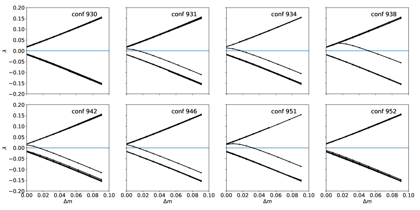
Figure 1: Examples of the identification of eigenvalues of $\hat{Q}$ crossing as the strange-quark mass is increased by $\Delta m$. We plot measurements on close-by configurations from the S400r001 run. The value of $\Delta m$ at which zero is crossed is a measure for the eigenvalue $-\lambda$ of $D(m_{\mathrm{s}})$. Note that crossings occur when the other eigenvalues have at least doubled their value, again indicated by the increased gap in the other eigenvalues.

4.2 Numerical results

The result of the analysis for ensembles with $n_{\mathrm{neg}}>0$ is collected in Table 2. We give the probability to find a configuration with a negative strange fermion determinant $\langle n_{\mathrm{neg}}\rangle$. We note that we did not encounter a single configuration with two negative real eigenvalues of the strange Dirac operator. In general, we find that the problem occurs so rarely that it is difficult to quantify the probability of configurations with negative real eigenvalues. Taking into account all configurations investigated. and without proper error analysis, we observe $\langle n_{\mathrm{neg}}\rangle$ of roughly two percent at $\beta=3.4$ and $\beta=3.46$, on around $0.3\%$ of the configurations at $\beta=3.55$ and on only very few of the configurations ($\sim 0.05\%$) at $\beta=3.7$. As one would expect, negative real eigenvalues quickly become unlikely as the continuum limit is approached.

Of course, such a global view ignores the varying physical parameters, in particular the quark masses as well as the details of the algorithmic choices, like the twisted-mass reweighting parameter $\mu_{0}$, and the rational function used in the RHMC. We will discuss their impact in the next section.

Furthermore, the above statement ignores the impact of autocorrelations on such numbers. As becomes evident from Table 2, large values for $\langle n_{\mathrm{neg}}\rangle$ come with large autocorrelations in this quantity: once a negative real eigenvalue occurs, the Markov chain frequently gets stuck and therefore many such configurations are produced in a row. This does not mean, that these configurations are particularly likely. Indeed, the uncertainties of $\langle n_{\mathrm{neg}}\rangle$ are typically on the order of $100$%. It simply means that the runs are too short to determine these values precisely.

To illustrate this issue, we have collected Monte Carlo time histories of the number of negative eigenvalues in Figure 2. In fact, we find only few ensembles, where $n_{\mathrm{neg}}>0$ has been visited more than once.

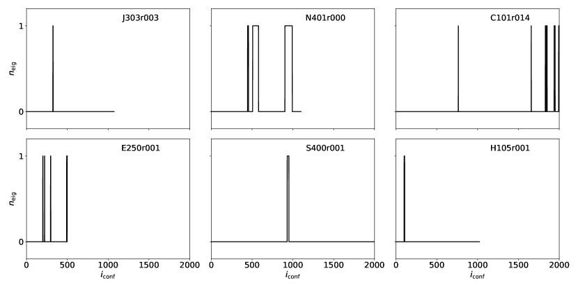
Figure 2: Monte Carlo time history of the number of negative real eigenvalues of the Dirac operator. Configurations are spaced by 4 units of molecular dynamics time; only for J303 this spacing amounts to 8 units. We observe that changes in the number are rare.

ens	$\langle n_{\mathrm{neg}}\rangle$	$\tau_{\mathrm{int}}$	$n_{\mathrm{sec}}$	$n_{\mathrm{max}}$	stat	$\mu_{0}$	$n_{\mathrm{out}}$	$n_{\mathrm{rat}}$	$r_{a},r_{b}$
H105r001	0.004(4)	2.0(4)	2	2	1023	0.001	10	11	[0.01,7.3]
H105r002	0.001(1)	0.50(3)	1	1	1042	0.001	10	11	[0.01,7.3]
H105r005	0.11(11)	45(22)	1	92	837	0.0005	7	13	[0.0032,7.6]
N101r001	0.11(11)	15(7)	1	30	280	0.0005	9	14	[0.0032,7.6]
C101r014	0.02(1)	6(1)	8	12	2000	0.0006	12	13	[0.006,7.8]
C101r015	0.09(9)	25(12)	6	33	601	0.0003	13	13	[0.006,7.8]
D101r005	0.03(3)	4(2)	1	9	286	0.0003	12	14	[0.006,7.8]
U103r002	0.09(9)	76(36)	1	154	1781	0.001	6	12	[0.0056,7.5]
U103r003	0.0005(5)	0.50(2)	1	1	1819	0.001	6	12	[0.0056,7.5]
U102r002	0.004(4)	7(1)	2	12	3562	0.002	6	12	[0.007,8.0]
N401r000	0.16(9)	35(16)	3	90	1100	0.00065	8	14	[0.002,7.5]
S400r000	0.01(1)	5(1)	1	10	872	0.00065	7	12	[0.01,7.3]
S400r001	0.01(1)	11(2)	1	21	2001	0.00065	7	12	[0.01,7.3]
E250r000	0.12(12)	8(4)	4	16	151	0.0001	14	14	[0.01,7.5]
E250r001	0.03(2)	3(1)	4	5	503	0.0001	15	14	[0.01,7.5]
J303r003	0.003(3)	1.5(3)	1	3	1073	0.00075	6	13	[0.008,7.0]

Table 2: Runs in which at least one config with $n_{\mathrm{neg}}\neq 0$ occurred. The probability of this event is given, together with its autocorrelation time. Note that the errors of these numbers have a very large uncertainty due to the long autocorrelations observed in some of the runs. As another measure of autocorrelations we give the number of sections in the chain with $n_{\mathrm{neg}}\neq 0$ denoted by $n_{sec}$, the length of the longest such region $n_{max}$ and the total statistics in number of configurations. We also list the twisted mass parameter $\mu_{0}$, the number of outer integrator steps $n_{out}$, and the parameters of the rational approximation. We observe a correlation of a lower number of outer integrator steps and longer stretches of $n_{\mathrm{neg}}\neq 0$.

5 Discussion

In the previous section, we have established that, in particular on the coarser lattices, there is a non-negligible frequency with which negative real eigenvalues of the strange Dirac operator occur.

A possible explanation of this occurrence could be the modification of the action by twisted-mass reweighting and the chosen RHMC function. Both increase the probability for small eigenvalues to appear in the ensembles (before applying the reweighting). However, we find that the mass shifts at which the crossings occur are typically large, of the order of twice the the spectral gap $\langle|\lambda_{\mathrm{min}}|\rangle$. This means that the negative eigenvalues of $D$ typically have (at least) the same magnitude as the smallest positive ones. Most of them are in a region, where the approximated action and the “exact” fermion determinant are almost the same. For the RHMC, the reweighting factors typically fluctuate on the percent level and, also for the twisted-mass reweighting factors, we do not observe a correlation between small values and a non-vanishing $n_{\mathrm{neg}}$.

Another possibility would be algorithmic instabilities or even an error in the simulation code. While both are hard to exclude, the rather consistent picture with the number of negative eigenvalues decreasing rapidly towards the continuum and no apparent correlation with volume, integrator step size, or acceptance rate does not make this a very convincing explanation.

Therefore our current working hypothesis is that the phenomenon described in this paper is a feature of the action. The fluctuations in the spectrum are simply larger than naively expected. The setup with the regularized actions is therefore necessary to reach these areas of configuration space and is essential for a correct simulation.

5.1 Autocorrelations

As already mentioned above, even with the regularized action a negative real eigenvalue has to cross a barrier in the action around $\lambda=0$ in order to disappear. This is linked with larger, fluctuating forces. In how far this is a problem depends on the choice of the integrator for the molecular dynamics equation of motion. With a precise enough integrator for the terms which are dominated by the contribution from small eigenvalues, the right momentum to get across the barrier is still needed, but the acceptance of such a trajectory will not suffer.

In the practical simulations on which this analysis is based, the force terms which receive most contributions from the smallest eigenvalues are most of the time tiny. They have therefore been integrated on a coarser time scale. If the associated step size if too large this can lead to poor acceptance of trajectories in which an eigenvalue has become very small or crossed zero.

That the tuning of such a setup can be delicate when there is a nonvanishing probability of negative real eigenvalues, is illustrated with two runs from the H105 ensemble. In runs r000 and r001, $\mu_{0}=0.001$ has been chosen along with an 11 pole rational approximation in the interval $[0.01,7.3]$. With the first term in the light quark product Eq. (3.9) and the two smallest poles of the RHMC on the outermost level, $10$ steps have led to an acceptance rate of $97\%$. This has to be compared to the choices taken for the r005 run. Here $\mu=0.0005$ along with a 13 pole rational function in $[0.0032,7.6]$ was used. Choosing 7 outer integration steps, again the first term of the light fermion forces and the three smallest $\bar{\mu}_{i}$ in the RHMC on the outer level, has led to an acceptance rate of $89\%$. We plot the corresponding regularizing functions in Figure 3.

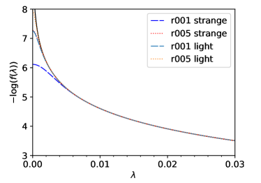
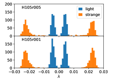
Figure 3: On the left, function for a single variable which replaces the $-\log(x)$ of the fermion action, for the light quark due to the twisted mass reweighting and for the strange due to the RHMC. We show the parameters of the H105r001 and H105r005 runs. Note that for the latter the potential barrier is roughly 1 unit higher. On the right we give the measured distribution of the lowest eigenvalue of $\hat{Q}$, not including the reweighting factors and without giving uncertainties, which are difficult to compute in the case of the H105r005 runs due to the large autocorrelations discussed in the text.

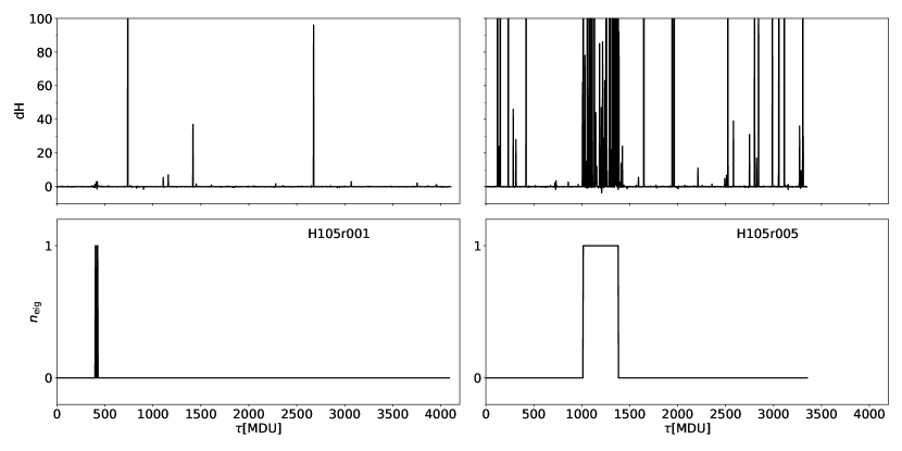
Figure 4: The violation of the HMC Hamiltonian in the top row is confronted with the number of negative eigenvalues of the Dirac operator in the bottom. We show the data for the runs H105r001 and H105r005. There is clear evidence that the period of poor acceptance, i.e. small $\exp(-dH)$ is correlated with the appearance of a negative real eigenvalue in the latter run. The different choice of molecular dynamics integrator might be responsible for the system staying in this state for an extended time.

At first sight, the three chains are equally acceptable. The reweighting factors were well behaved, with the twisted mass reweighting factors fluctuating less for r005 a expected. No signs of strange behavior in elementary observables were detected either. Only in the history of the energy violation of the molecular dynamics depicted in Figure 4, a long stretch of trajectories between number 1000 and 1500 with low acceptance has been observed.

It turns out that in this region, a negative real eigenvalue of the strange Dirac operator had developed. In this situation, it matters how accurately the terms with the smallest $\hat{\mu}_{i}$ are integrated, as they are dominated by the contributions from the smallest eigenvalues. Here we note that for the r005 run, we put more poles on the outer level of the integrator and we increased its step size significantly. The likely explanation is that trajectories which would have changed this eigenvalue’s sign were rejected, such that the system did not get out of this region.

Note that also in the other runs negative real eigenvalues were produced, but the system quickly moved away from these configurations. While these considerations are based on very low statistics, unavoidable by the nature of the problem, they do give a consistent picture. Note that from the point of view of tuning of the algorithm, this is an unpleasant situation, since the problem can even arise only after a significant portion of the full run. In hindsight, it would probably be better to use only a two-level scheme and not try to save computing time by using a further integrator level for these problematic forces.

5.2 Regularizing the action

As we have seen, the choice of the rational approximation and the quality of the integration of the associated forces has a determining impact on the problem discussed in this paper. Since one would naively expect that at a quark mass as large as the strange’s, the spectrum of $\hat{Q}^{2}$ can be confined to a region $[r_{a},r_{b}]$ in a practical simulation. Given the fast convergence of the Zolotarev approximation to $1/\sqrt{x}$, one then aims at choosing the number of poles and the range given by $r_{a}$ and $r_{b}$ such that no eigenvalue outside this interval will be encountered and the approximation error is negligible.

As has become clear from the findings presented here, this is a dangerous choice in that, both, decreasing $r_{a}$ and increasing $n_{\mathrm{rat}}$ improve the approximation but also heighten the obstacle at $\lambda=0$, which the eigenvalues have to overcome in order to get out of a region with a negative real eigenvalue.

These considerations can help understand the different behavior between the runs H105r001 and H105r005 discussed in the previous section. In Figure 3, we show as an illustration the function by which $-\log(\lambda)$, the contribution to the action of a single eigenvalue, is replaced due to the twisted mass regularization and the rational approximation. This needs to be compared with the distribution of the lowest eigenvalue given in the same figure.

As we see, for the strange quark the approximations do not differ in the region of the lowest eigenvalues of $\hat{Q}$. However, the maximum of the depicted functions at $\lambda=0$ is about one unit higher, making in much less likely to be overcome in a trajectory. Given these considerations, it seems advisable to fix $r_{a}$ and $r_{b}$ such that it covers the spectrum of $\hat{Q}^{2}$ apart from maybe some rare outliers which seem unavoidable in light of our findings while using a low order rational approximation such that one gets an acceptable fluctuation in the associated reweighting factors.

5.3 Light quarks

Negative real eigenvalues of the Dirac operator at the strange mass are also negative at the light-quark mass (if chosen below the strange’s mass-value). While the degeneracy of the two quark masses makes the product of the two determinants positive, the negative eigenvalues can still introduce large autocorrelations if the algorithm is inefficient in changing their sign.

In Figure 3 we compare functions with which the $-\log(\lambda)$ has been replaced in our setup for the runs H105r001/2 and H105r005. As can be seen, the fixed rational approximation acts quite similarly to the twisted mass reweighting, by chance the twisted mass parameters on the former runs give a function for one flavor which is almost identical to the rational approximation chosen for the latter.

Of course, it is not possible to deduce from the function alone whether or not there will be autocorrelation problems. It also depends on the typical distribution of the eigenvalues among other factors. In our analysis of the two algorithmic setups, we observe negative real eigenvalues of the light Dirac operator also on configurations, where this is not the case at the strange mass. However, also at the light-quark mass, at most one negative real eigenvalue occurs. These negative eigenvalues at the light-quark mass do not exhibit significant autocorrelations and (with the very limited statistics) on H105r001 are roughly twice as likely as at the strange-quark mass.

5.4 Effect of reweighting

With the (additional) reweighting factors equal to $\pm 1$ and the rare occurrence of the $-1$, it is obvious that their effect on the final observables will be small, at least as long as there is no strong correlation between the observable an the reweighting factor. If there is no correlation between the observable and reweighting factor, then the variance is not affected at all, see Eq. (5.4) of Ref. [26]. However, the autocorrelation problem discussed above can significantly impact the achievable accuracies, if a reliable error analysis is possible at all.

To illustrate the effect in a real situation, we again took the ensembles H105r001 and H105r002 and compared them to H105r005. These have the same physical parameters, but in the latter run the problem of negative real eigenvalues is much more pronounced.

For the pion mass, we extract $am_{\pi}=0.1213(12)$ from the former two ensembles and $am_{\pi}=0.1207(21)$ from the latter when we take the effect of the determinant’s sign into account. This is to be confronted with $0.1213(12)$ and $0.1220(17)$, respectively, without this reweighting factor. As expected, for the ensembles with very few negative signs of the determinant there is no significant difference, neither for the value, nor for the uncertainty. For r005, we observe a shift in the value which is somewhat smaller than the statistical uncertainty and also an increase in the error.

For the pseudoscalar decay constant the situation is essentially the same: on the first two ensembles it changes from 0.0763(10) without the signs to 0.0764(10) including them. On ${\tt r005}$ the respective numbers are 0.0758(9) and 0.0748(12).

6 Conclusions

On coarser lattices, the non-perturbatively improved Wilson Dirac operator at the strange-quark mass features negative real eigenvalues on a non-negligible subset of the configurations in the 2+1 flavor CLS ensembles. This has not been anticipated during the planning of the simulations, but the corresponding sign can be included in the measurement as a reweighting factor. We have described a robust but expensive way to compute this sign, however, it is difficult to exclude that occasionally a negative real eigenmode of the Dirac operator remains undetected. Since the effect of the reweighting seems to be rather small, we however assume that the effect of potentially missing a few such configurations would be even smaller.

The scenario observed also has consequences on the planning of the simulations. Specifically one needs to ensure that all regions of configuration space can be reached by the algorithm, even if one has the prejudice that some regions are not “relevant”. In the CLS ensembles, twisted-mass reweighting for the light quarks and the RHMC with fixed rational functions are employed to this end. However, for some of the runs, in hindsight, one should have used a larger value for the twisted mass parameter and/or fewer poles and smaller approximation range for the rational function. This would have made the transition of eigenvalues through zero easier and reduced autocorrelations. Also an integration scheme for the molecular dynamics equations of motion, where the forces dominated by the contributions of small eigenvalues of the Dirac operator are not put on a very coarse step size, seems advisable.

Note that one part of our action is not regulated: the diagonal term of the Dirac operator $\det D_{\mathrm{oo}}$. The fact that it turns out to be always positive might be due to the infinite barrier at zero determinant, rather than the actual physics of the system. This is impossible to tell after the simulation. As a side remark: this determinant is constant for unimproved Wilson fermions or the variant proposed in Ref. [27].

The practical ergodicity of Monte Carlo simulations remains difficult to assess in general, and it will always depend on the discretization and algorithms in question where possible difficulties might arise. Our discussion also highlights the fact that typical lattice simulations are not close to the continuum if it comes to details of the behavior of single eigenvalues of the Dirac operator.

Acknowledgements. We thank our CLS colleagues for providing the gauge field configurations this study is based on. We are indebted to Gunnar Bali, Mattia Bruno, Marco Cè, Georg von Hippel, Martin Lüscher, Teseo San José, Rainer Sommer, and Hartmut Wittig for very useful discussions. Eigenvalue calculations were performed on the HPC clusters “HIMster II” at the Helmholtz-Institut Mainz and “Mogon II” at JGU Mainz.

References

- [1] M. Clark and A. Kennedy, “Accelerating dynamical fermion computations using the rational hybrid Monte Carlo (RHMC) algorithm with multiple pseudofermion fields,” Phys.Rev.Lett., vol. 98, p. 051601, 2007.
- [2] R. Frezzotti and K. Jansen, “The PHMC algorithm for simulations of dynamical fermions: 1. Description and properties,” Nucl.Phys., vol. B555, pp. 395–431, 1999.
- [3] R. Frezzotti and K. Jansen, “The PHMC algorithm for simulations of dynamical fermions. 2. Performance analysis,” Nucl.Phys., vol. B555, pp. 432–453, 1999.
- [4] M. Bruno et al., “Simulation of QCD with N 2 1 flavors of non-perturbatively improved Wilson fermions,” JHEP, vol. 02, p. 043, 2015.
- [5] M. Bruno, T. Korzec, and S. Schaefer, “Setting the scale for the CLS flavor ensembles,” Phys. Rev., vol. D95, no. 7, p. 074504, 2017.
- [6] http://luscher.web.cern.ch/luscher/openQCD/.
- [7] M. Lüscher and F. Palombi, “Fluctuations and reweighting of the quark determinant on large lattices,” PoS, vol. LATTICE2008, p. 049, 2008.
- [8] M. Lüscher and S. Schaefer, “Lattice QCD with open boundary conditions and twisted-mass reweighting,” Comput.Phys.Commun., vol. 184, pp. 519–528, 2013.
- [9] G. Bergner and J. Wuilloud, “Acceleration of the Arnoldi method and real eigenvalues of the non-Hermitian Wilson-Dirac operator,” Comput. Phys. Commun., vol. 183, pp. 299–304, 2012.
- [10] K. G. Wilson, “Confinement of quarks,” Phys. Rev., vol. D10, pp. 2445–2459, 1974.
- [11] B. Sheikholeslami and R. Wohlert, “Improved continuum limit lattice action for QCD with Wilson fermions,” Nucl. Phys., vol. B259, p. 572, 1985.
- [12] M. Lüscher, S. Sint, R. Sommer, and P. Weisz, “Chiral symmetry and O() improvement in lattice QCD,” Nucl. Phys., vol. B478, pp. 365–400, 1996.
- [13] J. Bulava and S. Schaefer, “Improvement of lattice QCD with Wilson fermions and tree-level improved gauge action,” Nucl.Phys., vol. B874, pp. 188–197, 2013.
- [14] T. A. DeGrand, “A Conditioning Technique for Matrix Inversion for Wilson Fermions,” Comput.Phys.Commun., vol. 52, pp. 161–164, 1988.
- [15] A. M. Ferrenberg and R. H. Swendsen, “New monte carlo technique for studying phase transitions,” Phys. Rev. Lett., vol. 61, pp. 2635–2638, Dec 1988.
- [16] S. Duane, A. Kennedy, B. Pendleton, and D. Roweth, “Hybrid Monte Carlo,” Phys.Lett., vol. B195, pp. 216–222, 1987.
- [17] M. Lüscher and S. Schaefer, “Lattice QCD without topology barriers,” JHEP, vol. 1107, p. 036, 2011.
- [18] D. Mohler, S. Schaefer, and J. Simeth, “CLS 2+1 flavor simulations at physical light- and strange-quark masses,” EPJ Web Conf., vol. 175, p. 02010, 2018.
- [19] G. S. Bali, E. E. Scholz, J. Simeth, and W. Söldner, “Lattice simulations with improved Wilson fermions at a fixed strange quark mass,” Phys. Rev., vol. D94, no. 7, p. 074501, 2016.
- [20] Lüscher, Martin, “Topology, the Wilson flow and the HMC algorithm,” PoS, vol. LATTICE2010, p. 015, 2010.
- [21] M. Hasenbusch, “Speeding up the hybrid Monte Carlo algorithm for dynamical fermions,” Phys.Lett., vol. B519, pp. 177–182, 2001.
- [22] M. Hasenbusch and K. Jansen, “Speeding up lattice QCD simulations with clover improved Wilson fermions,” Nucl.Phys., vol. B659, pp. 299–320, 2003.
- [23] I. P. Omelyan, I. M. Mryglod, and R. Folk, “Symplectic analytically integrable decomposition algorithms: classification, derivation, and application to molecular dynamics, quantum and celestial mechanics simulations,” Computer Physics Communications, vol. 151, no. 3, pp. 272 – 314, 2003.
- [24] A. Stathopoulos and J. R. McCombs, “PRIMME: PReconditioned Iterative MultiMethod Eigensolver: Methods and software description,” ACM Transactions on Mathematical Software, vol. 37, no. 2, pp. 21:1–21:30, 2010.
- [25] L. Wu, E. Romero, and A. Stathopoulos, “Primme_svds: A high-performance preconditioned SVD solver for accurate large-scale computations,” CoRR, vol. abs/1607.01404, 2016.
- [26] M. Bruno, P. Korcyl, T. Korzec, S. Lottini, and S. Schaefer, “On the extraction of spectral quantities with open boundary conditions,” PoS, vol. LATTICE2014, p. 089, 2014.
- [27] A. Francis, P. Fritzsch, M. Lüscher, and A. Rago, “Master-field simulations of -improved lattice QCD: Algorithms, stability and exactness,” 2019.