Fast Encoding of AG Codes over $C_{ab}$ Curves

Abstract

We investigate algorithms for encoding of one-point algebraic geometry (AG) codes over certain plane curves called $C_{ab}$ curves, as well as algorithms for inverting the encoding map, which we call “unencoding”. Some $C_{ab}$ curves have many points or are even maximal, e.g. the Hermitian curve. Our encoding resp. unencoding algorithms have complexity $\tilde{\mathcal{O}}(n^{3/2})$ resp. $\tilde{\mathcal{O}}(qn)$ for AG codes over any $C_{ab}$ curve satisfying very mild assumptions, where $n$ is the code length and $q$ the base field size, and $\tilde{\mathcal{O}}$ ignores constants and logarithmic factors in the estimate. For codes over curves whose evaluation points lie on a grid-like structure, for example the Hermitian curve and norm-trace curves, we show that our algorithms have quasi-linear time complexity $\tilde{\mathcal{O}}(n)$ for both operations. For infinite families of curves whose number of points is a constant factor away from the Hasse–Weil bound, our encoding and unencoding algorithms have complexities $\tilde{\mathcal{O}}(n^{5/4})$ and $\tilde{\mathcal{O}}(n^{3/2})$ respectively.

I Introduction

I-A Algebraic geometry codes

In the following $\mathbb{F}$ is any finite field, while $\mathbb{F}_{q}$ denotes the finite field with $q$ elements. An $\mathbb{F}$-linear $[n,k]$ code is a $k$-dimensional subspace $\mathcal{C}\subseteq\mathbb{F}^{n}$. A substantial part of the literature on codes deals with constructing codes with special properties, in particular high minimum distance in the Hamming metric. In this context, algebraic geometry (AG) codes, introduced by Goppa [12], have been very fruitful: indeed, we know constructive families of codes from towers of function fields whose minimum distance beat the Gilbert–Varshamov bound [38]. Roughly speaking, such codes arise by evaluating functions in points lying on a fixed algebraic curve defined over $\mathbb{F}$. The evaluation points should be rational, i.e., defined over $\mathbb{F}$.

The well-known Reed–Solomon (RS) codes constitute a particularly simple subfamily of AG codes. Arguably, after Reed–Solomon (RS) codes, the most famous class of AG codes is constructed using the Hermitian curve; the Hermitian curve is a maximal curve, i.e. the number of rational points meets the Hasse–Weil bound [36, Theorem 5.2.3]. It is an example of the much larger family of $C_{ab}$ curves, which are plane curves given by a bivariate polynomial equation $H(X,Y)\in\mathbb{F}[X,Y]$ with several additional regularity properties. These imply that the function field associated to a $C_{ab}$ curve has a single place at infinity, $P_{\infty}$, and any function with poles only at $P_{\infty}$ can be represented by a bivariate polynomial $f\in\mathbb{F}[x,y]$ whose degree is bounded by a function of the pole order at $P_{\infty}$. Here, $x$ and $y$ are two functions which satisfy $H(x,y)=0$ and hence $\mathbb{F}[x,y]$ is a quotient of $\mathbb{F}[X,Y]$.

This means that the computations needed for operating with one-point AG codes over $C_{ab}$ curves are much simpler than in the general AG code case. The most well-studied operation pertaining to codes is decoding, i.e. obtaining a codeword from a noisy received word. For general AG codes, the fastest decoding algorithms essentially revert to linear algebra and have complexity roughly $\mathcal{O}(n^{3})$, where $n$ is the length of the code, e.g. [35, 23]. However, for one-point $C_{ab}$ codes, we have much faster algorithms, e.g. [1]. In [31], we studied Hermitian codes, i.e. AG codes over the Hermitian curve and obtained a decoding algorithm with complexity roughly $\tilde{\mathcal{O}}(n^{5/3})$.

I-B Encoding and unencoding

A simpler, though somewhat less studied problem for AG codes, however, is the encoding, i.e. the computational task of obtaining a codeword $\bm{c}\in\mathcal{C}$ belonging to a given message $\bm{m}\in\mathbb{F}^{k}$. Given a message $\bm{m}$ and a generator matrix $G\in\mathbb{F}^{k\times n}$ of the code, a natural encoder is obtained as the vector-matrix product $\bm{c}=\bm{m}G$. In general, this costs roughly $2kn$ operations in the field $\mathbb{F}$. If $G$ is “systematic”, e.g. in row-reduced echelon form, then it is slightly cheaper, costing only $2k(n-k)$ operations. Keeping the rate $k/n$ fixed and letting $n\rightarrow\infty$, the asymptotic cost is in both cases $\mathcal{O}(n^{2})$ operations in $\mathbb{F}$. For an arbitrary linear code, there is not much hope that we should be able to do better.

The inverse process of encoding, which we will call unencoding, matches a given codeword $\bm{c}$ with the sent message $\bm{m}$. If the encoder was systematic, this is of course trivial, but for an arbitrary linear encoder computing this inverse requires finding an information set for the code and inverting the generator matrix at those columns. This matrix inverse can be precomputed, in which case the unencoding itself is simply a $k\times k$ vector-matrix multiplication costing $\mathcal{O}(k^{2})$, which for a fixed rate equals $\mathcal{O}(n^{2})$.

In this article, we contribute to the study of fast encoding and unencoding by investigating the case of one-point AG codes over any $C_{ab}$ curve. For such codes, encoding can be considered as follows: the entries of the message $\bm{m}\in\mathbb{F}^{k}$ are written as the coefficients of a bivariate polynomial $f_{\bm{m}}\in\mathbb{F}[X,Y]$ with bounded degree, and the codeword is then obtained by evaluating $f_{\bm{m}}$ at rational points of the $C_{ab}$ curve (in some specific order). This is called a “ multipoint evaluation” of $f_{\bm{m}}$. Similarly, for unencoding we are given a codeword $\bm{c}\in\mathbb{F}^{n}$ and we seek the unique polynomial $f\in\mathbb{F}[X,Y]$ whose monomial support satisfies certain constraints and such that the entries of $\bm{c}$ are the evaluations of $f$ at the chosen rational points of the $C_{ab}$ curve. This is called “polynomial interpolation” of the entries of $\bm{c}$. Using this approach, we give fast algorithms for encoding and unencoding AG codes over any $C_{ab}$ curve; in particular we obtain quasi-linear complexity $\tilde{\mathcal{O}}(n)$ in the code length for encoding and unencoding one-point Hermitian codes.

Our outset is to find algorithms for multipoint evaluation and interpolation of bivariate polynomials on any point set $\mathcal{P}$, where we at first do not use the fact that $\mathcal{P}$ are rational points on a $C_{ab}$ curve; we do this in Sections III-A and IV-A respectively. Under mild assumptions, our algorithms for these problems have quasi-linear complexity in the input size when $\mathcal{P}$ is a “semi-grid”, i.e. if we let $\mathcal{Y}_{\alpha}=\{\beta\in\mathbb{F}\mid(\alpha,\beta)\in\mathcal{P}\}$ for $\alpha\in\mathbb{F}$, then each $|\mathcal{Y}_{\alpha}|$ is either 0 or equals some constant $\nu_{Y}$ independent of $\alpha$, see Figure 2 and Definition II.5. This result may be of independent interest. We then apply these algorithms to the coding setting in Sections III-B and IV-B respectively. In Section V we more specifically study the performance for $C_{ab}$ curves with special structure or sufficiently many points.

Contributions

• We give quasi-linear time algorithms for bivariate multipoint evaluation and interpolation when the point set is a semi-grid, under some simple conditions of the monomial support. See Remarks III.2 and IV.6.

• We give algorithms for encoding and for unencoding a one-point AG code over an arbitrary $C_{ab}$ curve. Under very mild assumptions on the $C_{ab}$ curve, these algorithms have complexity $\tilde{\mathcal{O}}(an)\subset\tilde{\mathcal{O}}(n^{3/2})$, respectively $\tilde{\mathcal{O}}(qn)$, where $a$ is the smallest nonzero element of the Weierstrass semigroup at $P_{\infty}$. Note $q<n$ for $C_{ab}$ curves of interest to coding theory. Our interpolation algorithm requires a polynomial amount of precomputation time. The encoding is not systematic. See Theorems III.4 and IV.12.

• We show that for codes whose evaluation points are semi-grids in a particular “maximal” way compared to the $C_{ab}$ curve, both algorithms have quasi-linear complexity $\tilde{\mathcal{O}}(n)$. This includes codes over the Hermitian curve and norm-trace curves. See Definitions V.1, V.2, V.5, V.6, V.7 and V.8.

• We show that the algorithms have improved complexity if the $C_{ab}$ curve has sufficiently many rational points. For example, if the number of rational points is a constant fraction from the Hasse–Weil bound, then the encoding algorithm has complexity $\tilde{\mathcal{O}}(n^{5/4})$, and the unencoding algorithm has complexity $\tilde{\mathcal{O}}(n^{3/2})$, see Theorem V.11.

I-C Related work on encoding

For the particularly simple case of RS codes, it is classical that the encoding can be done in quasi-linear complexity [18] using univariate multipoint evaluation (also see Section II-C).

Certain AG codes are investigated in [14], where they give a space-efficient encoding algorithm (i.e. it does not need to store a $k\times n$ generator matrix) using Gröbner bases and high-order automorphisms of the code; the time complexity, however, still remains quadratic.

In [42] one-point Hermitian codes over $\mathbb{F}_{q^{2}}$ are encoded by viewing them as concatenated RS codes. More precisely, if $f\in L(mP_{\infty})$, then $f=\sum_{i=0}^{\kappa}f_{i}(x)y^{i}$ for suitable polynomials $f_{i}(x)$, where $\kappa=\min(q-1,\lfloor m/(q+1)\rfloor)$. Evaluation of the $f_{i}(x)$ corresponds to fast encoding of RS codes. Since for each $x$-coordinate in $\mathbb{F}_{q^{2}}$ there are exactly $q$ points on the Hermitian curve with this $x$-coordinate, the encoding of the $f_{i}(x)$ gives rise to a $q$-fold concatenation of an RS codeword. Then the evaluation of $f_{i}(x)y^{i}$ is computed by multiplying each coordinate of the concatenated RS codeword with a suitable value. They perform complexity analysis, but it seems that using fast RS encoding the algorithm costs $\tilde{\mathcal{O}}(\kappa qq^{2})\subset\tilde{\mathcal{O}}(q^{4})=\tilde{\mathcal{O}}(n^{4/3})$ operations in $\mathbb{F}_{q^{2}}$. Though the underlying principle of our algorithm has similarities with this approach, our algorithm is a factor $n^{1/3}$ faster for the Hermitian curve.

In [34] the results of [42] are generalized to arbitrary one-point AG codes. Unfortunately, no asymptotic complexity analysis is given, making it difficult to compare their results with ours in terms of the parameters $n,k$ etc. Their abstract does state that there are examples where their method is three times as fast as the trivial quadratic encoding, and so one may suspect that they have no asymptotic gain in the general case. It can also be shown that their algorithm is never quasi-linear, which ours is in certain cases.

In [30] an encoding algorithm is given which is faster than $\mathcal{O}(n^{3/2})$ for certain carefully tailored, asymptotically good sub-codes of AG codes arising from the Garcia-Stichtenoth tower [10]. Our methods do not handle these codes, so the results can not be directly compared.

I-D Related work on bivariate multipoint evaluation

As outlined above, multipoint evaluation (MPE) and interpolation of bivariate polynomials over given point sets is a computational problem tightly related to encoding and unencoding of AG codes over $C_{ab}$ curves. In fact, any MPE algorithm for bivariate polynomials can immediately be applied for encoding. The situation is somewhat more complicated for interpolation, which we get back to. In this section and the next we review the literature on these problems.

We begin by discussing the MPE problem. The input is a point set $\mathcal{P}\subset\mathbb{F}^{2}$ and $f\in\mathbb{F}[X,Y]$ with $\deg_{X}f=d_{X}$ and $\deg_{Y}f=d_{Y}$, and we seek $\big{(}f(P)\big{)}_{P\in\mathcal{P}}$. Let $n:=|\mathcal{P}|$. As we will see in Section II-A, the main interest for the application of $C_{ab}$ codes is when $d_{X}d_{Y}<n$ and $d_{Y}\ll d_{X}$. The former is a common assumption in the literature, but numerous papers assume $d_{X}\approx d_{Y}$ and such algorithms will often have poor performance in our case.

Spurred by the quasi-linear algorithm available in the univariate case (see Section II-C), the best we could hope for would be an algorithm of complexity $\tilde{\mathcal{O}}(d_{X}d_{Y}+n)$, i.e. quasi-linear in the size of the input, but such a result is still not known in general. We will exemplify the complexities here for use in encoding Hermitian codes, i.e. $C_{ab}$ codes over the Hermitian curve, see Section V-A1: in this case $n=q^{3}$ where we work over the field $\mathbb{F}_{q^{2}}$. We will consider the case where the dimension of the code is in the order of the length, for which we then have $\deg_{X}f\in\mathcal{O}(n^{2/3})$ and $\deg_{Y}f<q=n^{1/3}$. The naive approach is to compute the evaluations of $f$ one-by-one. Using Horner’s rule, each such evaluation can be computed in $\mathcal{O}(d_{X}d_{Y})$ time, for a total complexity of $\mathcal{O}(d_{X}d_{Y}n)$. For the Hermitian codes, the complexity would be $\mathcal{O}(n^{2})$.

One of the first successes was obtained by Pan [33] with a quasi-linear algorithm for the case $\mathcal{P}=S_{X}\times S_{Y}$ for $S_{X},S_{Y}\subseteq\mathbb{F}$, i.e. evaluation on a grid, see Figure 1. The algorithm works by applying univariate MPE in a “tensored” form. The algorithm can be directly applied for any $\mathcal{P}$ by calling it on the smallest grid $\hat{\mathcal{P}}$ which contains all of $\mathcal{P}$ and then throwing away the unneeded evaluations. If $|\hat{\mathcal{P}}|\gg n$ then the complexity of this approach will not be quasi-linear in the original input size: in the worst case $|\hat{\mathcal{P}}|\approx n^{2}$ so the complexity becomes $\tilde{\mathcal{O}}(d_{X}d_{Y}+n^{2})$, which is quadratic in the input size when $d_{X}d_{Y}<n$. For Hermitian codes, then $\hat{\mathcal{P}}=\mathbb{F}_{q^{2}}^{2}$, hence Pan’s algorithm would give complexity $\tilde{\mathcal{O}}(n^{4/3})$. Our MPE algorithm presented in Section III-A essentially generalizes Pan’s algorithm to achieve quasi-linear cost on point sets with only semi-grid structure, see Figure 2; therefore the performance of our algorithm is never worse than Pan’s. Moreover, though few $C_{ab}$ curves form a grid, we observe in Section V-A that certain nice families, including the Hermitian curve, form semi-grids, implying that our evaluation algorithm has quasi-linear complexity for codes over these curves.

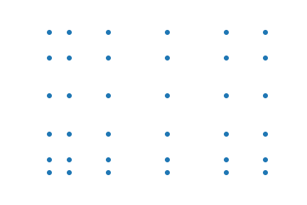
Figure 1: A grid.

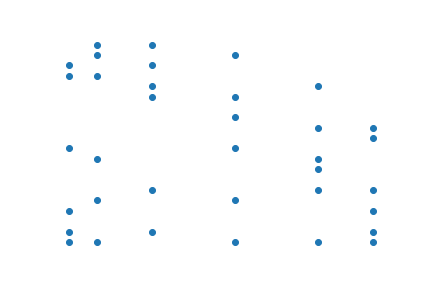
Figure 2: A semi-grid.

Nüsken and Ziegler [32] (NZ) reduced bivariate multipoint evaluation to a variant of bivariate modular composition: Write $\mathcal{P}=\{(\alpha_{1},\beta_{1}),\ldots,(\alpha_{n},\beta_{n})\}$ and assume all the $\alpha_{i}$ are distinct. Compute $h(X)=\prod_{i=1}^{n}(X-\alpha_{i})$ and $g\in\mathbb{F}[X]$ such that $g(\alpha_{i})=\beta_{i}$ for $i=1,\ldots,n$; both of these can be computed in $\tilde{\mathcal{O}}(n)$ time. If we then compute $\rho(x)=f(x,g(x))\operatorname{rem}h(x)\in\mathbb{F}[X]$, we see that $\rho(\alpha_{i})=f(\alpha_{i},\beta_{i})$ for each $i$, and hence we can compute the evaluations of $f$ at the points $\mathcal{P}$ by a univariate MPE of $\rho$ at the $\alpha_{1},\ldots,\alpha_{n}$. The latter can be done in $\tilde{\mathcal{O}}(n)$ time, so all that remains is the computation of $\rho(X)$. Nüsken and Ziegler show how to do this in complexity roughly $\mathcal{O}(d_{X}d_{Y}^{1.635+\epsilon}+nd_{Y}^{0.635+\epsilon})$, where $\epsilon>0$ can be chosen arbitrarily small, using fast rectangular matrix multiplication [21].

In general, and in the case of our interest, the $X$-coordinates of $\mathcal{P}$ will not be distinct. In this case, the points can be “rotated” by going to an extension field $K$ with $[K:\mathbb{F}]=2$: choose any $\theta\in K\setminus\mathbb{F}$, and apply the map ${(\alpha,\beta)}\longmapsto\enspace{(\alpha+\theta\beta,\beta)}$ to the points $\mathcal{P}$, and replace $f$ by $\hat{f}:=f(X-\theta Y,Y)$. We can now apply the NZ algorithm; that the operations will take place in $K$ costs only a small constant factor compared to operations in $\mathbb{F}$ since the extension degree is only $2$. The main problem is that $\deg_{Y}\hat{f}$ is now generically $\max(d_{X},d_{Y})$, so assuming $d_{Y}<d_{X}$, the complexity of the NZ algorithm becomes roughly $\mathcal{O}((n+d_{X}^{2})d_{X}^{0.635+\epsilon})$. For Hermitian codes, this yields $\mathcal{O}(n^{1.756+\epsilon})$.

In their celebrated paper [19], Kedlaya and Umans (KU) gave an algorithm for bivariate MPE with complexity $\mathcal{O}((n+d_{X}^{2})^{1+\epsilon})$ bit operations for any $\epsilon>0$, assuming $d_{Y}<d_{X}$. In outline, the algorithm works over prime fields by lifting the data to integers, then performing the MPE many times modulo many small primes, and then reassembling the result using the Chinese Remainder theorem. Over extension fields, some more steps are added for the lift to work. Note that the KU algorithm has quasi-linear complexity when $d_{Y}\approx d_{X}$. As mentioned, our main interest is $d_{Y}\ll d_{X}$. For our running example of the Hermitian code, applying the KU algorithm has complexity $\mathcal{O}(n^{4/3+\epsilon})$.

I-E Related work on bivariate interpolation

Let us turn to the interpolation problem. The input is now a point set $\mathcal{P}\subset\mathbb{F}^{2}$ and interpolation values $\mathcal{F}:\mathcal{P}\rightarrow\mathbb{F}$, and we seek $f\in\mathbb{F}[X,Y]$ such that $f(P)=\mathcal{F}(P)$ for each $P\in\mathcal{P}$. There are infinitely many such $f$, so to further restrict, or even make the output unique, one has to pose restrictions on the monomial support on the output $f$. We discuss the setting relevant to us in Section II-B.

Efficient interpolation algorithms include Pan’s [33], which works for points on grids, and its generalization by van der Hoeven and Schost [40], which works for certain structured subsets of grids. The monomial support output by these algorithms does not match our requirements. Given a $\hat{f}\in\mathbb{F}[X,Y]$ which correctly interpolates the sought values, but has incorrect monomial support, a general way to solve the problem is to let $\mathcal{G}\subset\mathbb{F}[X,Y]$ be the ideal of all polynomials which vanish at the points of $\mathcal{P}$, and then precompute a Gröbner basis $G$ of $\mathcal{G}$ under an appropriate monomial order: then $\hat{f}\operatorname{rem}G$, the unique remainder of $\hat{f}$ divided by the basis $G$, will have “minimal” possible monomial support under this order. One may use van der Hoeven’s fast division algorithm [39] for this step. This is exactly the strategy we use in Section IV-A2, where we first compute an $\hat{f}$ by generalizing Pan’s interpolation algorithm to work for semi-grids. This $\hat{f}$ can be described by a closed-form expression, see Lemma IV.1. A similar expression was used in a decoding algorithm for AG codes over the Hermitian curve in [25], and it was shown in [31] how to compute it fast; that approach can be seen as a special case of our algorithm.

A very different, and very flexible, interpolation algorithm is simply to solve the interpolation constraints as a system of linear constraints in the coefficients to the monomials in the monomial support. Solving the resulting $n\times n$ linear system using Gaussian elimination would cost $\mathcal{O}(n^{\omega})$, where $\omega<2.37286$ is the exponent of matrix multiplication [22]. In our case, we can do much better by observing that for the monomial support we require, the linear system would have low displacement rank, namely $a$, so we could use the algorithm for structured system solving by Bostan et al. [4, 3] for a cost of $\tilde{\mathcal{O}}(a^{\omega-1}n)$. For the Hermitian codes this yields a complexity of roughly $\tilde{\mathcal{O}}(n^{1.458})$, which is much slower than ours. However, for general $C_{ab}$ codes this is our main contender, and we compare again in Sections IV-B and V-B: the take-away is that for most parameters of interest, our algorithm seems to be faster.

II Preliminaries

II-A Codes from $C_{ab}$ curves

In this subsection we discuss in some detail the family of AG codes for which we want to find fast encoders and unencoders. Note that these AG codes and the algebraic curves used to construct them were previously studied in [26, 27]; these results will be mentioned here. Also they occur as a special case of the codes and curves studied in [8, 15].

For a bivariate polynomial $H=\sum_{i,j}a_{ij}X^{i}Y^{j}\in\mathbb{F}[X,Y]$ with coefficients in a finite field $\mathbb{F}$, we define $\operatorname{supp}(H)=\{X^{i}Y^{j}\mid a_{ij}\neq 0\}.$

Definition II.1.

Let $a,b$ be positive, coprime integers. We say that a bivariate polynomial $H\in\mathbb{F}[X,Y]$ is a $C_{ab}$ polynomial if:

• $X^{b},Y^{a}\in\operatorname{supp}(H)$,

• $X^{i}Y^{j}\in\operatorname{supp}(H)\implies ai+bj\leq ab$,

• The ideal $\langle{H,\frac{\partial{H}}{\partial{X}},\frac{\partial{H}}{\partial{Y}}}\rangle\subseteq\mathbb{F}[X,Y]$ is equal to the unit ideal $\mathbb{F}[X,Y]$.

Remark II.2.

In our algorithms the two variables $X$ and $Y$ are treated differently, which entails that complexities are not invariant under swapping of $X$ and $Y$ in $H$. We will commit to the arbitrary choice of “orienting” our algorithms such that their complexities depend explicitly only on $a$, which means that whenever the input is not assumed to have special structure which depends on $a$ and $b$, it is of course sensible to swap $X$ and $Y$ so $a\leq b$. Note that the case $a=b$ can only occur when $a=b=1$ since they are coprime. We will disregard this degenerate case.

Define $\deg_{a,b}$ to be the $(a,b)$-weighted degree of a bivariate polynomial. More concretely: $\deg_{a,b}(X^{i}Y^{j})=ai+bj$. The first two conditions imply that $H(X,Y)=\alpha X^{b}+\beta Y^{a}+G(X,Y),$ where $\alpha,\beta\in\mathbb{F}\setminus\{0\}$ and $\deg_{a,b}(G(X,Y))<ab.$ In particular, the polynomial $H$ is absolutely irreducible [15, Cor. 3.18]. The theory of Newton polygons, i.e., the convex hull of $\{(i,j)\mid X^{i}Y^{j}\in\operatorname{supp}(H)\}$, can also be used to conclude this [9].

This implies that the a $C_{ab}$ polynomial defines an algebraic curve. Following [26], the type of algebraic curves obtained in this way are called $C_{ab}$ curves. As observed there, these curves, when viewed as projective curves, have exactly one point at infinity $P_{\infty}$, which, if singular, is a cusp. What this means can be explained in a very simple way using the language of function fields. A given $C_{ab}$ polynomial $H$ defines a $C_{ab}$ curve, with function field $F=\mathbb{F}(x,y)$ obtained by extending the rational function field $\mathbb{F}(x)$ with a variable $y$ satisfying $H(x,y)=0$. Since $H$ is absolutely irreducible, $\mathbb{F}$ is the full constant field of $F.$ The statement that the point $P_{\infty}$, if it is a singularity, is a cusp, just means that the function $x$ has exactly one place of $F$ as a pole. With slight abuse of notation, we denote this place by $P_{\infty}$ as well. The defining equation of a $C_{ab}$ curve, directly implies that for any $i,j\in\mathbb{Z}$, the function $x^{i}y^{j}$ has pole order $\deg_{a,b}(x^{i}y^{j})=ai+bj$ at $P_{\infty}.$ In particular, $x$ has pole order $a$ and $y$ has pole order $b$ at $P_{\infty}.$

The genus of a function field is important for applications in coding theory, since it occurs in the Goppa bound on the minimum distance of AG codes. It is observed in [26] that the genus of the function field $F=\mathbb{F}(x,y)$ defined above equals $g=(a-1)(b-1)/2$. Indeed, this is implied by the third condition in Definition II.1, also see [2, Theorem 4.2]. We collect some facts in the following proposition. These results are contained in [26], expressed there in the language of algebraic curves.

Proposition II.3 ([26]).

Let $H\in\mathbb{F}[X,Y]$ be a $C_{ab}$ polynomial and $F=\mathbb{F}(x,y)$ the corresponding function field. Then $F$ has genus $g=\frac{1}{2}(a-1)(b-1).$ The place $P_{\infty}$ is rational and a common pole of the functions $x$ and $y$ and in fact the only place which is a pole of either $x$ or $y$. For any $i,j\in\mathbb{Z}$, the function $x^{i}y^{j}\in F$ has pole order $\deg_{a,b}(x^{i}y^{j})=ai+bj$ at $P_{\infty}.$

For a divisor $D$ of the function field $F$, we denote by $\mathcal{L}(D)$ the Riemann–Roch space associated to $D$. The third condition in Definition II.1 implies that a $C_{ab}$ curve cannot have singularities, apart from the possibly singular point at infinity. This has two important consequences. In the first place, all rational places of $F$ distinct from $P_{\infty}$, can be identified with the points $(\alpha,\beta)\in\mathbb{F}^{2}$ satisfying $H(\alpha,\beta)=0$. We will call these places the finite rational places of $F$. Throughout the paper we will, by a slight abuse of notation, use a finite place $P_{\alpha,\beta}$ and its corresponding rational point $(\alpha,\beta)$ interchangeably. A second consequence, as observed in [26], is that the functions in $\mathbb{F}[x,y]$ are the only functions in $F$ with poles only at $P_{\infty}$; in other words, $\mathcal{L}(mP_{\infty})=\{f\in\mathbb{F}[x,y]\mid\deg_{a,b}(f)\leq m\}$. Since $H(x,y)=0$, any $f\in\mathbb{F}[x,y]$ can be uniquely written as a polynomial with $y$-degree at most $a-1$. We will call this the standard form of $f$. We are now ready to define $C_{ab}$ codes.

Definition II.4.

Let $H$ be a $C_{ab}$ polynomial and $F$ the corresponding function field. Further, let $P_{1},\ldots,P_{n}$ be distinct, finite rational places of $F$ and let $m$ be a non-negative integer. Then the $C_{ab}$ code of order $m$ is defined to be:

$$\mathcal{C}_{H}(\mathcal{P},m) :=\{{(\operatorname{ev}_{\mathcal{P}}(f)}\enspace|\enspace{f\in\mathcal{L}(mP_{\infty})}\}\subseteq\mathbb{F}^{n}\ ,\textrm{ where}$$

$$\operatorname{ev}_{\mathcal{P}}(f) =\big{(}f(P_{1}),\ldots,f(P_{n})\big{)}\ .$$

In the standard notation for AG codes used for example in [36], the code $\mathcal{C}_{H}(\mathcal{P},m)$ is equal to the code $C_{\mathcal{L}}(D,mP_{\infty}),$ with $D=P_{1}+\cdots+P_{n}.$ Since the divisor $mP_{\infty}$ is a multiple of a single place, the codes $\mathcal{C}_{H}(\mathcal{P},m)$ are examples of what are known as one-point AG codes. Using for example [36, Theorem 2.2.2], we obtain that $\mathcal{C}_{H}(\mathcal{P},m)$ is an $[n,k,d]$ linear code, where $k=\dim\big{(}\mathcal{L}(mP_{\infty})\big{)}-\dim\big{(}\mathcal{L}(mP_{\infty}-D)\big{)}$ and $d\geq n-m.$ In particular, $k=n$ if $m>n+2g-2$. Therefore we will from now on always assume that $m\leq n+2g-1.$ If $m<n,$ then $k=\dim\big{(}\mathcal{L}(mP_{\infty})\big{)}\geq m+1-g$ and if additionally $2g-2<m$, then $k=m+1-g.$ The precise minimum distance of a $C_{ab}$ code is in general not known from just the defining data. Lastly, we also note the obvious bound $n\leq q^{2}$, where $q=|\mathbb{F}|$, due to the identification of rational places with points in $\mathbb{F}^{2}$.

When comparing algorithms pertaining to AG codes, as well as many other types of codes, it is customary to assume that the dimension $k$ grows proportional to $n$, denoted $k\in\Theta(n)$, i.e. that the rate goes to some constant as $n\rightarrow\infty$. For any such family of $C_{ab}$ codes this implies that $m\in\Theta(n)$. This in turn means that any message polynomial $f\in\mathcal{L}(mP_{\infty})$ in standard form satisfies $\deg_{Y}f<a$ and $\deg_{X}f<m/a\in\Theta(n/a)$. For most interesting $C_{ab}$-codes the genus $g\ll n$, so $ab\ll n$, while $n$ is relatively large compared to $q$, as measured e.g. against the Hasse–Weil bound, see Section V-B. This means that in the cases of most interest to us, the message polynomials tend to have very different $X$ and $Y$ degrees.

II-B The evaluation-encoding map

An encoding for a linear code such as $\mathcal{C}_{H}(\mathcal{P},m)$ is a linear, bijective map $\phi:\mathbb{F}^{k}\rightarrow\mathcal{C}_{H}(\mathcal{P},m)\subseteq\mathbb{F}^{n}$. Computing the image of $\phi$ for some $\bm{m}\in\mathbb{F}^{k}$ is called “encoding” $\bm{m}$. The process of computing the inverse, i.e. given a codeword $\bm{c}\in\mathcal{C}_{H}(\mathcal{P},m)$ recover the message $\bm{m}:=\phi^{-1}(\bm{c})$, is often unnamed in the literature. For lack of a better term (and since “decoding” is reserved for error-correction), we will call it “unencoding”.

In light of Definition II.4, we can factor $\phi$ as $\phi=\operatorname{ev}_{\mathcal{P}}\circ\varphi$, where $\varphi:\mathbb{F}^{k}\rightarrow\mathcal{L}(mP_{\infty})$ is linear and injective. If we choose $\varphi$ sufficiently simple and such that it outputs elements of $\mathbb{F}[x,y]$ in standard form, the computational task of applying $\phi$ reduces to computing $\operatorname{ev}_{\mathcal{P}}$, i.e. multipoint evaluation of bivariate polynomials of $(a,b)$-weighted degree at most $m$. A natural basis for $\mathcal{L}(mP_{\infty})$ is

$$B=\{x^{i}y^{j}\mid\deg_{a,b}(x^{i}y^{j})\leq m\land j\leq a-1\}\ .$$ (II.1)

If $k=\dim(\mathcal{L}(mP_{\infty}))$, then $|B|=k$, and we therefore choose $\varphi$ as taking the elements of a message $\bm{m}$ as the coefficients to the monomials of this basis in some specified order. Then applying $\varphi$ takes no field operations at all.

If $k<\dim(\mathcal{L}(mP_{\infty}))$ then $|B|>k$, and this may happen when $m\geq n$. We should then choose a subset $\hat{B}\subset B$ of $k$ monomials such that the vectors $\{\operatorname{ev}_{\mathcal{P}}(x^{i}y^{j})\}_{x^{i}y^{j}\in\hat{B}}$ are linearly independent. For our encoding algorithms, the choice of $\hat{B}$ will not matter. However, for unencoding, we will assume that this choice has been made so that the monomials in $\hat{B}$ are, when sorted according to their $(a,b)$-weighted degrees, lexicographically minimal. Put another way, a monomial $x^{i}y^{j}\in B$ is not in $\hat{B}$ exactly when there is a polynomial $g\in\ker(\operatorname{ev}_{\mathcal{P}})$ with $\operatorname{\mathsf{LM}}_{\operatorname{\preceq_{\mathit{a,b}}}}(g)=x^{i}y^{j}$, where $\operatorname{\mathsf{LM}}_{\operatorname{\preceq_{\mathit{a,b}}}}$ denotes leading monomial according to $\operatorname{\preceq_{\mathit{a,b}}}$, the $(a,b)$ weighted degree breaking ties by $x^{b}\operatorname{\preceq_{\mathit{a,b}}}y^{a}$. Such monomials $x^{i}y^{j}$ are what we will call “reducible” monomials in Section IV-A2.

$\hat{B}$ is easy to precompute: start with $\hat{B}=\emptyset$, and go through the monomials of $B$ in order of increasing $(a,b)$-weighted degree. For each such $x^{u}y^{v}$ if $\operatorname{ev}_{\mathcal{P}}(x^{u}y^{v})$ is linearly independent from $\{\operatorname{ev}_{\mathcal{P}}(x^{i}y^{j})\}_{x^{i}y^{j}\in\hat{B}}$, then add to $\hat{B}$.

II-C Notation and computational tools

For any point set $\mathcal{P}\subseteq\mathbb{F}^{2}$ we define $\mathcal{X}(\mathcal{P}):=\{{\alpha\in\mathbb{F}}\enspace|\enspace{\exists\beta\in\mathbb{F}\operatorname{\enspace s.t.\enspace}(\alpha,\beta)\in\mathcal{P}}\}$, i.e. the set of all $X$-coordinates that occur in $\mathcal{P}$. We write $n_{X}(\mathcal{P}):=\lvert\mathcal{X}(\mathcal{P})\rvert$ for the number of distinct $X$-coordinates. Similarly, for any $\alpha\in\mathbb{F}$ we define $\mathcal{Y}_{\alpha}(\mathcal{P}):=\{{\beta\in\mathbb{F}}\enspace|\enspace{(\alpha,\beta)\in\mathcal{P}}\}$, i.e. the set of $Y$-coordinates that occur for a given $X$-coordinate $\alpha$, and we let

$$\nu_{Y}(\mathcal{P}):=\max_{\alpha\in\mathcal{P}}\lvert\mathcal{Y}_{\alpha}(\mathcal{P})\rvert.$$

In discussions where it is clear from the context which point set $\mathcal{P}$ we are referring to, we may simply write $\mathcal{X},\mathcal{Y},n_{X},\nu_{Y}$. Note that if $\mathcal{P}$ is a subset of the rational points of a $C_{ab}$ curve with polynomial $H(X,Y)$, then $\nu_{Y}(\mathcal{P})\leq a=:\deg_{Y}(H)$ since for any given value of $\alpha$, there are at most $a$ solutions to the resulting equation in $H(\alpha,Y)$.

Definition II.5.

A point set $\mathcal{P}\subset\mathbb{F}^{2}$ is a semi-grid if $|\mathcal{Y}_{\alpha}(\mathcal{P})|\in\{0,\nu_{Y}(\mathcal{P})\}$ for each $\alpha\in\mathbb{F}$.

As outlined in Section II-A, we distinguish between the bivariate polynomial ring $\mathbb{F}[X,Y]$ and the subset of functions in the $C_{ab}$ function field spanned by $x$ and $y$, denoted $\mathbb{F}[x,y]$. However, there is a natural inclusion map of functions $f\in\mathbb{F}[x,y]$ in standard form into a polynomial $f(X,Y)\in\mathbb{F}[X,Y]$ of $Y$-degree less than $a$. In discussions and algorithms, we sometimes abuse notation by more or less explicitly making use of this inclusion map.

For ease of notation, our algorithms use lookup tables, also known as dictionaries or associative arrays. This is just a map $\mathcal{A}\rightarrow\mathcal{B}$ between a finite set $\mathcal{A}$ and a set $\mathcal{B}$ but where all the mappings have already been computed and stored, and hence can quickly be retrieved. We use the notation $\mathcal{F}\in\mathcal{B}^{\mathcal{A}}$ to mean a lookup table from $\mathcal{A}$ to $\mathcal{B}$. For $a\in\mathcal{A}$, we write $\mathcal{F}[a]\in\mathcal{B}$ for the mapped value stored in $\mathcal{F}$. Note that this is for notational convenience only: all our uses of lookup tables could be replaced by explicit indexing in memory arrays, and so we will assume that retrieving or inserting values in tables costs $O(1)$.

Our complexity analyses count basic arithmetic operations in the field $\mathbb{F}$ on an algebraic RAM model. We denote by $\mathsf{M}(n)$ the cost of multiplying two univariate polynomials in $\mathbb{F}[X]$ of degree at most $n$. We can take $\mathsf{M}(n)\in O(n\log n\log\log n)$ [5], or the slightly improved algorithm of [13] with cost $\mathsf{M}(n)\in O(n\log n\ 8^{\log^{*}n})$, both of which are in $\tilde{\mathcal{O}}(n)$. For precision, our theorems state complexities in big-$\mathcal{O}$ including all log-factors, and we then relax the expressions to soft-$\mathcal{O}$ for overview.

Our algorithms take advantage of two fundamental computational tools for univariate polynomials: fast multipoint evaluation and fast interpolation. These are classical results, see e.g. [41, Corollaries 10.8 and 10.12].

Proposition II.6.

There exists an algorithm $\mathsf{UnivariateMPE}$ which inputs a univariate polynomial $h\in\mathbb{F}[Z]$ and evaluation points ${\mathcal{S}}\subseteq\mathbb{F}$, and outputs a table $\mathcal{F}:\mathbb{F}^{\mathcal{S}}$ such that $\mathcal{F}[\alpha]=h(\alpha)$ for every $\alpha\in{\mathcal{S}}$. It has complexity

$$\mathcal{O}(\mathsf{M}(\deg h+\lvert{\mathcal{S}}\rvert)\log({\deg h+\lvert{\mathcal{S}}\rvert}))\subset\tilde{\mathcal{O}}(\deg h+\lvert{\mathcal{S}}\rvert)$$

operations in $\mathbb{F}$.

Proposition II.7.

There exists an algorithm $\mathsf{UnivariateInterp}_{Z}$ which inputs evaluation points ${\mathcal{S}}\subseteq\mathbb{F}$ and evaluation values $\mathcal{F}\in\mathbb{F}^{{\mathcal{S}}}$, and outputs the unique $f\in\mathbb{F}[Z]$ such that $\deg f<k$ and $f(\alpha)=\mathcal{F}[\alpha]$ for each $\alpha\in{\mathcal{S}}$, where $k=|{\mathcal{S}}|$. It has complexity $\mathcal{O}(\mathsf{M}(k)\log({k}))\subset\tilde{\mathcal{O}}(k)$ operations in $\mathbb{F}$.

III A fast encoding algorithm

Let us now consider an algorithm for computing the encoding map for $C_{ab}$ codes. We are given a message vector $f\in\mathcal{L}(mP_{\infty})\subset\mathbb{F}[X,Y]/\langle{H}\rangle$ and $n$ finite rational places $P_{1},\ldots,P_{n}$ of $F$; we wish to compute $f(P_{1}),\ldots,f(P_{n})$. We translate this problem into bivariate polynomial multipoint-evaluation by lifting $f$ to a polynomial in $\mathbb{F}[X,Y]$ in standard form, and identifying each $P_{i}$ with a pair $(\alpha_{i},\beta_{i}),\in\mathbb{F}^{2}$ such that $H(\alpha_{i},\beta_{i})=0$ for $i=1,\ldots,n$. In the following subsection we will focus on the evaluation problem at hand, while in Section III-B we will apply the results to encoding of codes over $C_{ab}$ curves.

III-A Multipoint-Evaluation of Bivariate Polynomials

Let us for now forget that we originally came from the setting of codes. Suppose that we are given a set $\mathcal{P}\subseteq\mathbb{F}^{2}$ of points with $\lvert\mathcal{P}\rvert=n$ and a bivariate polynomial $f\in\mathbb{F}[X,Y]$ with $\deg_{X}f=d_{X}$ and $\deg_{Y}f=d_{Y}$. This naive approach will have complexity $\mathcal{O}(nd_{X}d_{Y})$.

We will generalize Pan’s multipoint evaluation algorithm [33] (see Section I-D), and show that it performs well on point sets $\mathcal{P}$ where most $|\mathcal{Y}_{\alpha}(\mathcal{P})|$ are roughly the same size for each $\alpha\in\mathcal{X}(\mathcal{P})$.

The idea of the algorithm is the following: we write

$$f(X,Y)=f_{0}(X)+f_{1}(X)Y+\ldots+f_{d_{Y}}(X)Y^{d_{Y}}\quad,f_{i}\in\mathbb{F}[X]\ ,$$

and then proceed by $d_{Y}+1$ univariate multipoint evaluations of the polynomials $f_{i}(X)$, $i=0,\ldots,d_{Y}$, each evaluated on the values $\mathcal{X}(\mathcal{P})$. For each $\alpha\in\mathcal{X}(\mathcal{P})$, we can therefore construct a univariate polynomial in $Y$ without further computations:

$$g_{\alpha}(Y)=f_{0}(\alpha)+f_{1}(\alpha)Y+\ldots+f_{d_{Y}}(\alpha)Y^{d_{Y}}\quad,f_{i}\in\mathbb{F}[X]\ .$$

Again using univariate multipoint evaluation, we obtain $g_{\alpha}(\beta)=f(\alpha,\beta)$ for each $\beta\in\mathcal{Y}_{\alpha}(\mathcal{P})$. For the algorithm listing see Algorithm 1.

Input:

Bivariate polynomial $f=f_{0}(X)+f_{1}(X)Y+\ldots+f_{d_{Y}}(X)Y^{d_{Y}}\in\mathbb{F}[X,Y]$.

Evaluation points $\mathcal{P}\subseteq\mathbb{F}^{2}$.

Output:

Evaluation values $\mathcal{F}=(f(\alpha,\beta))_{(\alpha,\beta)\in\mathcal{P}}\in\mathbb{F}^{\mathcal{P}}$.

1 $\mathcal{X}\leftarrow\mathcal{X}(\mathcal{P})$

2 $\mathcal{Y}_{\alpha}\leftarrow\mathcal{Y}_{\alpha}(\mathcal{P})$

3 for $i=1,\ldots,d_{Y}$ do $\mathcal{F}_{i}\leftarrow\mathsf{UnivariateMPE}(f_{i},\mathcal{X})\in\mathbb{F}^{\mathcal{X}}$

4 foreach $\alpha\in\mathcal{X}$ do

5       $g_{\alpha}\leftarrow\sum_{i=0}^{d_{Y}}\mathcal{F}_{i}[\alpha]Y^{i}\in\mathbb{F}[Y]$

6       $\mathcal{G}_{\alpha}\leftarrow\mathsf{UnivariateMPE}(g_{\alpha},\mathcal{Y}_{\alpha})\in\mathbb{F}^{\mathcal{Y}_{\alpha}}$

7      

8return $\mathcal{F}\leftarrow(\mathcal{G}_{\alpha}[\beta])_{(\alpha,\beta)\in\mathcal{P}}\in\mathbb{F}^{\mathcal{P}}$.

Algorithm 1 $\mathsf{BivariateMPE}$: Bivariate multipoint evaluation

Theorem III.1.

Algorithm 1 is correct. It has complexity

$$\mathcal{O}(d_{Y}\mathsf{M}(d_{X}+n_{X})\log({d_{X}+n_{X}})+n_{X}\mathsf{M}(d_{Y}+\nu_{Y})\log({d_{Y}+\nu_{Y}}))\subset\tilde{\mathcal{O}}(d_{Y}d_{X}+n_{X}(d_{Y}+\nu_{Y}))$$

operations in $\mathbb{F}$, where $d_{X}=\deg_{X}f$, $n_{X}=n_{X}(\mathcal{P})$, and $\nu_{Y}=\nu_{Y}(\mathcal{P})$.

Proof.

Correctness follows from the fact that

$$\mathcal{F}[\alpha,\beta]=\mathcal{G}_{\alpha}[\beta]=g_{\alpha}(\beta)=\sum_{i=0}^{d_{Y}}\mathcal{F}_{i}[\alpha]\beta^{i}=\sum_{i=0}^{d_{Y}}f_{i}(\alpha)\beta^{i}=f(\alpha,\beta)\ .$$

For the complexity, Algorithms 1 and 1 both have cost $\mathcal{O}(n)$. Proposition II.6 implies that computing $\mathcal{F}_{i}$ costs

$$\mathcal{O}(\mathsf{M}(\deg f_{i}+n_{X})\log({\deg f_{i}+n_{X}}))\text{ for }i=1,\ldots,d_{Y}\ ,$$

thus the total cost for Algorithm 1 becomes

$$\mathcal{O}(d_{Y}\mathsf{M}(d_{X}+n_{X})\log({d_{X}+n_{X}})).$$

Algorithm 1 costs no operations in $\mathbb{F}$. From Proposition II.6 it follows that computing each $\mathcal{G}_{\alpha}$ costs

$$\mathcal{O}(\mathsf{M}(d_{Y}+\lvert\mathcal{Y}_{\alpha}\rvert)\log({d_{Y}+\lvert\mathcal{Y}_{\alpha}\rvert}))\text{ for }\alpha\in\mathcal{X},$$

thus the total cost of Algorithm 1 becomes

$$\mathcal{O}(n_{X}\mathsf{M}(d_{Y}+\nu_{Y})\log({d_{Y}+\nu_{Y}}))\ .$$

Algorithm 1 costs no operations in $\mathbb{F}$, and so the total cost of computing $\mathcal{F}$ becomes as in the theorem. ∎

Remark III.2.

If $\mathcal{P}\in\mathbb{F}^{2}$ is a semi-grid, and $f\in\mathbb{F}[X,Y]$ is a dense polynomial satisfying either $n_{X}\in\mathcal{O}(\deg_{X}f)$ or $\deg_{Y}(f)\in\mathcal{O}(\nu_{Y})$, then Algorithm 1 has quasi-linear complexity in the input size $|\mathcal{P}|+\deg_{X}f\deg_{Y}f$.

Remark III.3.

Even if we use classical polynomial multiplication, with $\mathsf{M}(n)=\mathcal{O}(n^{2})$, and if we assume $d_{X}\in\Theta(n_{X})$ and $d_{Y}\in\Theta(\nu_{Y})$, then the cost of Algorithm 1 is $\tilde{\mathcal{O}}(\nu_{Y}^{2}n_{X}+\nu_{Y}n_{X}^{2})$ which for most point sets is better than the naive approach of point-by-point evaluation costing $\mathcal{O}(\nu_{Y}n_{X}n)$.

III-B Fast encoding

Algorithm 1 gives rise a fast encoder; details can be found in Algorithm 2.

Input: A $C_{ab}$ code $\mathcal{C}_{H}(\mathcal{P},m)\subseteq\mathbb{F}^{n}$ of dimension $k$, with $\mathcal{P}=\{P_{1},\ldots,P_{n}\}$ being finite rational places. Message $\bm{m}\in\mathbb{F}^{k}$.

Output: Codeword $\bm{c}=\phi(\bm{m})$, where $\phi:\mathbb{F}^{k}\rightarrow\mathcal{C}_{H}(\mathcal{P},m)$ is the encoding map defined in Section II-B.

1 $f\leftarrow\varphi(\bm{m})\subset\mathbb{F}[x,y]$ in standard form, where $\varphi$ is as in Section II-B

2 $\mathcal{F}\leftarrow\mathsf{BivariateMPE}(f,\mathcal{P})\in\mathbb{F}^{\mathcal{P}}$, where $f$ is lifted to $\mathbb{F}[X,Y]$

return $(\mathcal{F}[P_{1}],\ldots,\mathcal{F}[P_{n}])\in\mathbb{F}^{n}$

Algorithm 2 $\mathsf{Encode}$

Theorem III.4.

Algorithm 2 is correct. It uses at most $\mathcal{O}(\mathsf{M}(m+an_{X})\log({m+an_{X}}))\subset\tilde{\mathcal{O}}(m+an_{X})$ operations in $\mathbb{F}$, where $n_{X}=n_{X}(\mathcal{P})$.

Proof.

Correctness follows trivially from Theorem III.1. For complexity let $d_{X}=\deg_{X}f$, $d_{Y}=\deg_{Y}f$ and $\nu_{Y}=\nu_{Y}(\mathcal{P})$. Since $f$ is in standard form we have that $d_{Y}<a$. Furthermore, since $f\in\mathcal{L}(mP_{\infty})$ we know that $ad_{X}+bd_{Y}\leq m$. It follows that $d_{X}d_{Y}<d_{X}a\leq m$. Since for each value of $X$ in $\mathcal{X}(\mathcal{P})$, there can be at most $a$ solutions in $Y$ to the $C_{ab}$ curve equation, we know $\nu_{Y}<a$. It follows from Theorem III.1 that the cost of Algorithm 2 is

$$\mathcal{O}(d_{Y}\mathsf{M}(d_{X}+n_{X})\log({d_{X}+n_{X}})+n_{X}\mathsf{M}(d_{Y}+\nu_{Y})\log({d_{Y}+\nu_{Y}}))$$

$$\subset\mathcal{O}(\mathsf{M}(m+an_{X})\log({m+an_{X}}))\ .$$

∎

As can be seen, the complexity of this algorithm depends on parameters of the $C_{ab}$ curve compared to the code length as well as the layout of the evaluation points: more specifically on how $an_{X}$ compares with the code length $n$. In Section V-A we will revisit the complexity for codes over $C_{ab}$ curves that lie on semi-grids as well as $C_{ab}$ curves which have many points. In the worst case, the following corollary bounds the complexity in terms of the length of the code under very mild assumptions on the $C_{ab}$ curve. Note that this cost is still much better than encoding using a matrix-vector product in $\mathcal{O}(n^{2})$ time.

Corollary III.5.

In the context of Algorithm 2, let $q$ be the cardinality of $\mathbb{F}$ and assume $n\geq q$. Assume further that the genus $g$ of the $C_{ab}$ curve satisfies $g\leq n$. Then the complexity of Algorithm 2 is $\tilde{\mathcal{O}}(q\sqrt{n})\subset\tilde{\mathcal{O}}(n^{3/2})$.

Proof.

There can at most be $q$ different $X$-coordinates in $\mathcal{P}$, so $n_{X}\leq q$. Assuming w.l.o.g that $a<b$ we get $n\geq g=\tfrac{1}{2}(a-1)(b-1)\geq\tfrac{1}{2}(a-1)^{2}$, and hence $a\leq\sqrt{2n}+1\in\mathcal{O}(\sqrt{n})$. Lastly, $m\leq n+2g-1\in\mathcal{O}(n)$. The result follows from Theorem III.4. ∎

IV A fast unencoding algorithm

We now consider the problem of unencoding: we are given a codeword $\bm{c}\in\mathcal{C}_{H}(\mathcal{P},m)$ and we wish to find the message $\bm{m}=\phi^{-1}(\bm{c})\in\mathbb{F}^{k}$, where $\phi$ is the encoding map defined in Section II-B. Following the discussion there, we factor $\phi$ as $\phi=\operatorname{ev}_{\mathcal{P}}\circ\varphi$, where $\varphi:\mathbb{F}^{k}\mapsto\mathcal{L}(mP_{\infty})$ which is a linear map that sends unit vectors to monomials in

$$\hat{B}\subseteq B:=\{x^{i}y^{j}\mid\deg_{a,b}(x^{i}y^{j})\leq m\land j\leq a-1\}\ .$$

Recall that the evaluation map is injective on $\mathcal{L}(mP_{\infty})$ whenever $m<n$, so in this case $\hat{B}=B$. Otherwise, $\hat{B}$ is chosen such that if $g\in\ker(\operatorname{ev}_{\mathcal{P}})$, then $\operatorname{\mathsf{LM}}_{\operatorname{\preceq_{\mathit{a,b}}}}(g)\notin\hat{B}$, where $\operatorname{\preceq_{\mathit{a,b}}}$ is the $(a,b)$-weighted degree monomial order, breaking ties by $x^{b}\operatorname{\preceq_{\mathit{a,b}}}y^{a}$.

In Section IV-A we will first rephrase the above as a general interpolation problem for bivariate polynomials, and not use the fact that the $\mathcal{P}$ are a subset of a low-degree $C_{ab}$ curve. In Section IV-B we specialise and analyse the complexity of using this approach for the unencoding problem.

IV-A Interpolation of Bivariate Polynomials

In the following subsections, we suppose that we are given a set of $n$ points $\mathcal{P}\subseteq\mathbb{F}^{2}$, not necessarily lying on a $C_{ab}$ curve, and a corresponding collection of values $\mathcal{F}\in\mathbb{F}^{\mathcal{P}}$. The interpolation problem consists of finding a polynomial $f\in\mathbb{F}[X,Y]$ such that $f(\alpha,\beta)=\mathcal{F}[\alpha,\beta]$ for all $(\alpha,\beta)\in\mathcal{P}$. Since there are many such polynomials, one usually imposes constraints on the set of monomials $X^{i}Y^{j}$ that may appear with non-zero coefficient in $f$. For us, the relevant monomial support is the set $\hat{B}$ described above.

Depending on $\mathcal{P}$ and the allowed monomial support, not all interpolation conditions can be satisified, but whenever they can, the solution could be found in time $O(n^{2})$ using linear algebra, by precomputing a basis for the inverse of the evaluation map.

This section details a faster approach. In Section IV-A we first use an efficient recursive algorithm to find an $\hat{f}\in\mathbb{F}[X,Y]$ such that $\hat{f}(x(P_{i}),y(P_{i}))=c_{i}$ for $i=1,\ldots,n$ while $\deg_{Y}\hat{f}<a$. In general, $\hat{f}(x,y)$ is not the sought $f$ since its monomial support will be too large. However, $f\in\hat{f}+\mathcal{G}$, where $\mathcal{G}$ is the ideal of polynomials in $\mathbb{F}[X,Y]$ vanishing at the points $P_{1},\ldots,P_{n}$. By the choice of $\hat{B}$, we will see that we can recover $f$ by reducing $\hat{f}$ modulo a suitable Gröbner basis $G$ of $\mathcal{G}$ using a fast multivariate division algorithm.

IV-A1 Finding a structured interpolation polynomial

We will use the following explicit equation which finds an interpolating polynomial $\hat{f}\in\mathbb{F}[X,Y]$ with $\deg_{Y}\hat{f}<\nu_{Y}(\mathcal{P})$ and $\deg_{X}\hat{f}<n_{X}(\mathcal{P})$. Our algorithm for efficiently computing this polynomial essentially generalizes Pan’s interpolation algorithm [33], which was designed to work for points on grids, to work for points on semi-grids.

Lemma IV.1.

Given a point set $\mathcal{P}\in\mathbb{F}^{2}$ and interpolation values $\mathcal{F}\in\mathbb{F}^{\mathcal{P}}$, then $\hat{f}\in\mathbb{F}[X,Y]$ given by

$$\hat{f}=\sum_{\alpha\in\mathcal{X}}\prod_{\alpha^{\prime}\in\mathcal{X}\setminus\{{\alpha}\}}\frac{X-\alpha^{\prime}}{\alpha-\alpha^{\prime}}\sum_{\beta\in\mathcal{Y}_{\alpha}}\mathcal{F}[\alpha,\beta]\prod_{\beta^{\prime}\in\mathcal{Y}_{\alpha}\setminus\{{\beta}\}}\frac{Y-\beta^{\prime}}{\beta-\beta^{\prime}}\ ,$$ (IV.1)

satisfies $f(\alpha,\beta)=\mathcal{F}[\alpha,\beta]$ for all $(\alpha,\beta)\in\mathcal{P}$.

Proof.

Let $(\alpha,\beta)\in\mathcal{P}$. Then the only nonzero term in the first sum is the one corresponding to $\alpha$, while the only nonzero term in the second sum is the one corresponding to $\beta$, thus

$$\hat{f}(\alpha,\beta)=\prod_{\alpha^{\prime}\in\mathcal{X}\setminus\{{\alpha}\}}\frac{\alpha-\alpha^{\prime}}{\alpha-\alpha^{\prime}}\mathcal{F}[\alpha,\beta]\prod_{\beta^{\prime}\in\mathcal{Y}_{\alpha}\setminus\{{\beta}\}}\frac{\beta-\beta^{\prime}}{\beta-\beta^{\prime}}=\mathcal{F}[\alpha,\beta]\ .$$

∎

Our strategy to compute $\hat{f}$ in an efficient manner can be viewed in the following way: we start by computing the polynomials $\hat{f}_{\alpha}:=\hat{f}(\alpha,Y)\in\mathbb{F}[Y]$ for every $\alpha\in\mathcal{X}$ using univariate interpolation. We then reinterpret our interpolation problem as being univariate over $(\mathbb{F}[Y])[X]$, i.e. we seek $\hat{f}(X)$ having coefficients in $\mathbb{F}[Y]$ and such that $\hat{f}(\alpha)=\hat{f}_{\alpha}$. However, to be more clear, and for a slightly better complexity (on the level of logarithms), we make this latter interpolation explicit.

Before we put these steps together to compute $\hat{f}$ in Algorithm 4, we therefore first consider the following sub-problem: Given any subset ${\mathcal{S}}\subseteq\mathbb{F}$ and a table of univariate polynomials $\mathcal{V}\in\mathbb{F}[Y]^{{\mathcal{S}}}$ indexed by ${\mathcal{S}}$, compute the following bivariate polynomial:

$$h(X,Y)=\sum_{\alpha\in{\mathcal{S}}}\mathcal{V}[\alpha]\prod_{\alpha^{\prime}\in{\mathcal{S}}\setminus\{{\alpha}\}}(X-\alpha^{\prime})\in\mathbb{F}[X,Y]\ .$$ (IV.2)

For the $(\mathbb{F}[Y])[X]$ interpolation, we will follow an approach of univariate interpolation closely mimicking that of [41, Chapter 10.2]. Firstly, we arrange the $X$-coordinates of the interpolation points in a balanced tree:

Definition IV.2.

Let ${\mathcal{S}}\subseteq\mathbb{F}$. A balanced partition tree of ${\mathcal{S}}$ is a binary tree which has subsets of ${\mathcal{S}}$ as nodes, and satisfies the following:

1. ${\mathcal{S}}$ is the root node.

2. A leaf node is a singleton set $\{\alpha\}\subseteq{\mathcal{S}}$.

3. An internal node $\mathcal{N}$ is the disjoint union of its two children $\mathcal{N}_{1},\mathcal{N}_{2}$ and they satisfy $\lvert\lvert\mathcal{N}_{1}\rvert-\lvert{\mathcal{N}_{2}}\rvert\rvert\leq 1$.

If $\mathcal{T}$ is a balanced partition tree and $\mathcal{N}\subseteq{\mathcal{S}}$, we will write $\mathcal{N}\in\mathcal{T}$ if $\mathcal{N}$ is a node of $\mathcal{T}$, and denote by $\mathcal{T}[\mathcal{N}]$ the set of its two child nodes.

Lemma IV.3 (Lemma 10.4 [41]).

There exists an algorithm $\mathsf{TreeVanish}_{X}$ which inputs a balanced partition tree $\mathcal{T}$ of some ${\mathcal{S}}\subseteq\mathbb{F}$ and outputs the lookup table

$$\mathsf{TreeVanish}_{X}(\mathcal{T}):=\big{(}\prod_{\alpha\in\mathcal{N}}(X-\alpha)\big{)}_{\mathcal{N}\in\mathcal{T}}\in\mathbb{F}[X]^{\mathcal{T}}.$$

The algorithm uses at most $\mathcal{O}(\mathsf{M}(k)\log(k))\subset\tilde{\mathcal{O}}(k)$ operations in $\mathbb{F}$, where $k=|{\mathcal{S}}|$.

Input: Points ${\mathcal{S}}\subseteq\mathbb{F}$, non-empty.

Lookup table $\mathcal{V}\in\mathbb{F}[Y]^{{\mathcal{S}}}$.

A balanced partition tree $\mathcal{T}$ with ${\mathcal{S}}\in\mathcal{T}$.

$\mathcal{U}=\mathsf{TreeVanish}_{X}(\mathcal{T})\in\mathbb{F}[X]^{\mathcal{T}}$.

Output: $h(X,Y)\in\mathbb{F}[X,Y]$ as in (IV.2).

1 if $S=\{{\alpha}\}$ then

2       return $\mathcal{V}[\alpha]\in\mathbb{F}[Y]$

3else

4       $\{{{\mathcal{S}}_{1},{\mathcal{S}}_{2}}\}\leftarrow\mathcal{T}[{\mathcal{S}}]$

5       for $k=1,2$ do

6             $\mathcal{V}_{k}\leftarrow(\mathcal{V}[\alpha])_{\alpha\in{\mathcal{S}}_{k}}\in\mathbb{F}[Y]^{{\mathcal{S}}_{k}}$

7             $\hat{f}_{k}\leftarrow\mathsf{Combine}({\mathcal{S}}_{k},\mathcal{V}_{k},\mathcal{T},\mathcal{U})\in\mathbb{F}[X,Y]$

8      return $\hat{f}_{1}\mathcal{U}[{\mathcal{S}}_{2}]+\hat{f}_{2}\mathcal{U}[{\mathcal{S}}_{1}]\in\mathbb{F}[X,Y]$

Algorithm 3 $\mathsf{Combine}$: $\mathbb{F}[Y]$-linear combination of vanishing polynomials

With these tools in hand, Algorithm 3 is an algorithm for computing $h(X,Y)$ as in (IV.2).

Theorem IV.4.

Algorithm 3 is correct. If $\deg_{Y}\mathcal{V[\alpha]}<d$ for all $\alpha\in{\mathcal{S}}$, then the algorithm has complexity $\mathcal{O}(d\mathsf{M}(k)\log({k}))\subset\tilde{\mathcal{O}}(dk)$ operations in $\mathbb{F}$, where $k=\lvert{\mathcal{S}}\rvert$.

Proof.

We prove correctness by induction on $\lvert{\mathcal{S}}\rvert$. The base case of ${\mathcal{S}}=\{\alpha\}$ is trivial. For the induction step, the algorithm proceeds into the else-branch and we note that $|{\mathcal{S}}_{1}|,|{\mathcal{S}}_{2}|<|{\mathcal{S}}|$ and so the induction hypothesis applies to $\hat{f}_{k}$ for $k=1,2$:

$$\hat{f}_{k}=\sum_{\alpha\in{\mathcal{S}}_{k}}\mathcal{V}_{k}[\alpha]\prod_{\alpha^{\prime}\in{\mathcal{S}}_{k}\setminus\{{\alpha}\}}(X-\alpha^{\prime})\ .$$

Note that $\mathcal{V}_{k}[\alpha]=\mathcal{V}[\alpha]$ and ${\mathcal{S}}_{1}\cup{\mathcal{S}}_{2}={\mathcal{S}}$, so we conclude that the polynomial returned by the algorithm is

$$\hat{f}_{1}\mathcal{U}[S_{2}]+\hat{f}_{2}\mathcal{U}[S_{1}]$$

$$=\sum_{\alpha\in{\mathcal{S}}_{1}}\mathcal{V}[\alpha]\prod_{\alpha^{\prime}\in{\mathcal{S}}\setminus\{{\alpha}\}}(X-\alpha^{\prime})+\sum_{\alpha\in{\mathcal{S}}_{2}}\mathcal{V}[\alpha]\prod_{\alpha^{\prime}\in{\mathcal{S}}\setminus\{{\alpha}\}}(X-\alpha^{\prime})$$

$$=\sum_{\alpha\in{\mathcal{S}}}\mathcal{V}[\alpha]\prod_{\alpha^{\prime}\in{\mathcal{S}}\setminus\{{\alpha}\}}(X-\alpha^{\prime})\ .$$

For complexity let $T(k)$ denote the cost of $\mathsf{Combine}$ for $\lvert{\mathcal{S}}\rvert=k$. At a recursive step we solve two subproblems of size at most $\lceil k/2\rceil$; and we compute the expression $\hat{f}_{1}\mathcal{U}[{\mathcal{S}}_{2}]+\hat{f}_{2}\mathcal{U}[{\mathcal{S}}_{1}]$. Since $\mathcal{U}[{\mathcal{S}}_{k}]\in\mathbb{F}[X]$ then each of the two products can be carried out using $\deg_{Y}\hat{f}_{k}+1\leq d$ multiplications in $\mathbb{F}[X]_{\leq k}$ and hence cost $\mathcal{O}(d\mathsf{M}(k))$ each. The addition $\hat{f}_{1}\mathcal{U}[{\mathcal{S}}_{2}]+\hat{f}_{2}\mathcal{U}[{\mathcal{S}}_{1}]$ costs a further $\mathcal{O}(dk)$. In total, we get the following recurrence relation:

$$T(k) =2T(k/2)+\mathcal{O}(d\mathsf{M}(k))\ .$$

This has the solution $T(k)=\mathcal{O}(d\mathsf{M}(k)\log({k}))+\mathcal{O}(k)T(1)$. $T(1)$ is the base case of the algorithm, and costs $\mathcal{O}(d)$. ∎

We are now in position to assemble the steps outlined for computing the interpolation polynomial given by Lemma IV.1 following the steps outlined above by supplying Algorithm 3 with the correct input; this is described in Algorithm 4.

Note that Algorithm 4 makes use of the subroutines $\mathsf{UnivariateInterp}_{Y}$ and $\mathsf{UnivariateMPE}$ that were introduced in Proposition II.6 and Proposition II.7.

Input: Points $\mathcal{P}\subseteq\mathbb{F}^{2}$, non-empty. Lookup table of interpolation values $\mathcal{F}\in\mathbb{F}^{\mathcal{P}}$.

Output: The polynomial $\hat{f}\in\mathbb{F}[X,Y]$ given by Lemma IV.1.

1 $\mathcal{X}\leftarrow\mathcal{X}(\mathcal{P})\subseteq\mathbb{F}$

2 foreach $\alpha\in\mathcal{X}$  do

3       $\mathcal{Y}_{\alpha}\leftarrow\mathcal{Y}_{\alpha}(\mathcal{P})\subseteq\mathbb{F}$

4       $\mathcal{F}_{\alpha}\leftarrow(\mathcal{F}[\alpha,\beta])_{\beta\in\mathcal{Y}_{\alpha}}\in\mathbb{F}^{\mathcal{Y}_{\alpha}}$

5       $\hat{f}_{\alpha}\leftarrow\mathsf{UnivariateInterp}_{Y}(\mathcal{Y}_{\alpha},\mathcal{F}_{\alpha})\in\mathbb{F}[Y]$

6      

7$\mathcal{T}\leftarrow$ a balanced partition tree of $\mathcal{X}$

8 $\mathcal{U}\leftarrow\mathsf{TreeVanish}_{X}(\mathcal{T})\in\mathbb{F}[X]^{\mathcal{T}}$

9 $g\leftarrow$ formal derivative of $\mathcal{U}[\mathcal{X}]\in\mathbb{F}[X]$

10 $\mathcal{R}\leftarrow\mathsf{UnivariateMPE}(g,\mathcal{X})\in\mathbb{F}^{\mathcal{X}}$

11 $\mathcal{V}\leftarrow(\hat{f}_{\alpha}/\mathcal{R}[\alpha])_{\alpha\in\mathcal{X}}\in\mathbb{F}[Y]^{\mathcal{X}}$

return $\mathsf{Combine}(\mathcal{X},\mathcal{V},\mathcal{T},\mathcal{U})$

Algorithm 4 $\mathsf{BivariateInterp}$: Bivariate interpolation

Theorem IV.5.

Algorithm 4 is correct. It has complexity

$$\mathcal{O}(\nu_{Y}\mathsf{M}(n_{X})\log({n_{X}})+n_{X}\mathsf{M}(\nu_{Y})\log({\nu_{Y}}))\subseteq\tilde{\mathcal{O}}(n_{X}\nu_{Y})$$

operations in $\mathbb{F}$, where $n_{X}=n_{X}(\mathcal{P})$ and $\nu_{Y}=\nu_{Y}(\mathcal{P})$.

Proof.

Denote by $\tilde{f}\in\mathbb{F}[X,Y]$ the polynomial returned by the algorithm and $\hat{f}$ the polynomial of Lemma IV.1, and we wish to prove $\tilde{f}=\hat{f}$. Note first that for any $\alpha\in\mathcal{X}$

$$\hat{f}(\alpha,Y)=\sum_{\beta\in\mathcal{Y}_{\alpha}}\mathcal{F}[\alpha,\beta]\prod_{\beta^{\prime}\in\mathcal{Y}_{\alpha}\setminus\{{\beta}\}}\frac{y-\beta^{\prime}}{\beta-\beta^{\prime}}=\hat{f}_{\alpha}\ ,$$

where $\hat{f}_{\alpha}$ is as computed in Algorithm 4. By the correctness of $\mathsf{Combine}$

$$\tilde{f}=\sum_{\alpha\in\mathcal{X}}\hat{f}_{\alpha}/\mathcal{R}[\alpha]\prod_{\alpha^{\prime}\in\mathcal{X}\setminus\{{\alpha}\}}(X-\alpha^{\prime})\ .$$

Since $g=\sum_{\alpha\in\mathcal{X}}\prod_{\alpha^{\prime}\in\mathcal{X}\setminus\{{\alpha}\}}(X-\alpha^{\prime})$ we have that

$$\mathcal{R}[\alpha]=\prod_{\alpha^{\prime}\in\mathcal{X}\setminus\{{\alpha}\}}(\alpha-\alpha^{\prime})\in\mathbb{F}\ ,\quad\alpha\in\mathcal{X}\ .$$

It follows that $\tilde{f}=\hat{f}$.

For complexity we observe that computing $\mathcal{T}$ in Algorithm 4 cost $\mathcal{O}(n_{X}\log(n_{X}))$, and $\mathcal{U}$ in Algorithm 4 costs $\mathcal{O}(\mathsf{M}(n_{X})\log({n_{X}}))$ by Lemma IV.3. Computing $g$ in Algorithm 4 costs $\mathcal{O}(n_{X})$ and $\mathcal{R}$ in Algorithm 4 costs $\mathcal{O}(\mathsf{M}(n_{X})\log({n_{X}}))$ by Proposition II.6. The total cost of computing all the $\hat{f}_{\alpha}$ for $\alpha\in\mathcal{X}$ in Algorithm 4 is $\mathcal{O}(n_{X}\mathsf{M}(\nu_{Y})\log({\nu_{Y}}))$ by Proposition II.7. Since $\mathcal{R}[\alpha]\in\mathbb{F}$, the division $\mathcal{V}$ in Algorithm 4 costs $\mathcal{O}(n_{X}\nu_{Y})$ operations, one for each of the $\deg\hat{f}_{\alpha}<\nu_{Y}$ coefficients in each of the $n_{X}$ polynomials $\hat{f}_{\alpha}$. Finally Algorithm 4 costs $\mathcal{O}(\nu_{Y}\mathsf{M}(n_{X})\log({n_{X}}))$ by Theorem IV.4. The total cost becomes as in the theorem. ∎

Remark IV.6.

If $\mathcal{P}$ is a semi-grid then Algorithm 4 has quasi-linear complexity in the input size $|\mathcal{P}|$. Furthermore, since the output polynomial $\hat{f}$ has $\deg_{X}\hat{f}<n_{X}$ and $\deg_{Y}\hat{f}<\nu_{Y}$, then the $n_{X}\nu_{Y}$-dimensional $\mathbb{F}$-vector space of polynomials satisfying such degree restrictions must be in bijection with the $n$-dimensional choice of values $\mathcal{F}$. Hence, Algorithm 4 returns the unique polynomial $\hat{f}$ satisfying these degree bounds and which interpolate the values. This is in contrast to the case where $\mathcal{P}$ is not a semi-grid, as we will discuss in the following section.

Remark IV.7.

If $\mathcal{P}$ is very far from being a semi-grid, the performance of the algorithm can sometimes be improved by a proper blocking-strategy in use of $\mathsf{Combine}$. For example, suppose that $\mathcal{X}=\{{\alpha_{1},\ldots,\alpha_{k}}\}$, and furthermore assume that $|\mathcal{Y}_{\alpha_{1}}|=\ldots=|\mathcal{Y}_{\alpha_{k-1}}|=1$ while $|\mathcal{Y}_{\alpha_{k}}|=k$, so that $n=2k-1\in\Theta(k)$. The cost of Algorithm 4 will therefore be $\tilde{\mathcal{O}}(k^{2})$. However, in this case we can split the points $\mathcal{P}$ into $\mathcal{P}_{1}:=\{{(\alpha,\beta)\in\mathcal{P}}\enspace|\enspace{\alpha\neq\alpha_{k}}\}$ and $\mathcal{P}_{2}:=\{{(\alpha,\beta)\in\mathcal{P}}\enspace|\enspace{\alpha=\alpha_{k}}\}$, and the interpolation values into $\mathcal{F}_{s}:=(\mathcal{F}[\alpha,\beta]/\gamma_{s})_{(\alpha,\beta)\in\mathcal{P}_{s}}\in\mathbb{F}^{\mathcal{P}_{s}}$ for $s=1,2$, where $\gamma_{s}:=\prod_{\alpha^{\prime}\in\mathcal{X}(\mathcal{P})\setminus{\mathcal{X}(\mathcal{P}_{s})}}(\alpha-\alpha^{\prime})$ have been precomputed. We can then compute $\hat{f}_{s}:=\mathsf{BivariateInterp}(\mathcal{P}_{s},\mathcal{F}_{s})$ and obtain the desired interpolating polynomial from Lemma IV.1 as follows:

$$\hat{f}=\sum_{s=1,2}\hat{f_{s}}\prod_{\alpha\in\mathcal{X}(\mathcal{P})\setminus{\mathcal{X}(\mathcal{P}_{s})}}(X-\alpha_{i}).$$

Not counting precomputation, the total cost of this approach becomes $\tilde{\mathcal{O}}(k)=\tilde{\mathcal{O}}(n)$.

IV-A2 Reducing the support

We now continue to deal with the problem that we wish to find an interpolation polynomial with a constrained monomial support. We do not deal with the completely general question but one relevant to unencoding $C_{ab}$ codes: we are given positive integers $a,b\in\mathbb{Z}_{>0}$ and seek an interpolation polynomial $f$ which is “reduced” in a specific way according to the monomial ordering $\operatorname{\preceq_{\mathit{a,b}}}$. We will use $\hat{f}$ from the preceding section as an initial approximation which we then transform into the sought polynomial.

In the following, we will use Gröbner bases and assume that the reader is familiar with the basic notions; see e.g. [6]. We will exclusively use the monomial order $\operatorname{\preceq_{\mathit{a,b}}}$, so to lighten notation, in this section we write $\operatorname{\mathsf{LM}}$ instead of $\operatorname{\mathsf{LM}}_{\operatorname{\preceq_{\mathit{a,b}}}}$. Given a point set $\mathcal{P}\in\mathbb{F}^{2}$, we will call a monomial $X^{i}Y^{j}$ “reducible” if there is a polynomial $h\in\mathbb{F}[X,Y]$ with $\operatorname{\mathsf{LM}}(h)=X^{i}Y^{j}$ and such that $h(P)=0$ for all $P\in\mathcal{P}$. In other words, we can “remove” $X^{i}Y^{j}$ from the support of $f$ by properly choosing $\alpha\in\mathbb{F}$ and setting $f:=f-\alpha h$, and this does not increase the leading monomial of $f$.

We would now like to address the following problem:

Problem IV.8.

Given a point set $\mathcal{P}\subseteq\mathbb{F}^{2}$ and $a,b\in\mathbb{Z}_{\geq 0}$, and a polynomial $\hat{f}\in\mathbb{F}[X,Y]$, compute a polynomial $f\in\mathbb{F}[X,Y]$ satisfying

$$f(P)=\hat{f}(P)\text{ for }P\in\mathcal{P}\ ,$$

and such that no monomial in the support of $f$ is reducible.

Note that the polynomial $f-\hat{f}$ vanishes at all points $\mathcal{P}$. It is therefore natural to investigate the ideal

$$\mathcal{G}=\{h\mid h(P)=0\text{ for }P\in\mathcal{P}\}\subseteq\mathbb{F}[X,Y]\ .$$ (IV.3)

In fact we have the following lemma, which follows immediately from standard properties of Gröbner bases, see e.g. [6, Theorem 3.3]:

Lemma IV.9.

In the context of IV.8, let $G$ be a Gröbner basis of $\mathcal{G}$ given in (IV.3) according to $\operatorname{\preceq_{\mathit{a,b}}}$. Then $f$ is the unique remainder of dividing $\hat{f}$ with $G$ using the multivariate division algorithm, i.e. $f=\hat{f}\operatorname{rem}G$.

Before we give an efficient algorithm for solving IV.8, the following lemma recalls some simple structure on weighted-degree Gröbner bases:

Lemma IV.10.

Let $\mathcal{P}\subset\mathbb{F}^{2}$ and $a,b\in\mathbb{Z}_{\geq 0}$, let $\mathcal{G}$ be given by (IV.3), and let $G=\{G_{1},\ldots,G_{t}\}$ be a minimal Gröbner basis of $\mathcal{G}$. Then $\deg_{Y}(\operatorname{\mathsf{LM}}(G_{i}))\neq\deg_{Y}(\operatorname{\mathsf{LM}}(G_{j}))$ for $i\neq j$. In particular, if $\mathcal{G}$ contains an element $g$ such that $\operatorname{\mathsf{LM}}(g)=Y^{A}$ for some $A\in\mathbb{Z}_{\geq 1}$, then $|G|=t\leq A+1$.

Proof.

Assume oppositely that $\deg_{Y}(\operatorname{\mathsf{LM}}(G_{i}))=\deg_{Y}(\operatorname{\mathsf{LM}}(G_{j}))$ for $i\neq j$, then either $\operatorname{\mathsf{LM}}(G_{i})\mid\operatorname{\mathsf{LM}}(G_{j})$ or $\operatorname{\mathsf{LM}}(G_{j})\mid\operatorname{\mathsf{LM}}(G_{i})$. Both of these contradict that $G$ is minimal.

Assume now w.l.o.g. that $\deg_{Y}(\operatorname{\mathsf{LM}}(G_{1})<\ldots<\deg_{Y}(\operatorname{\mathsf{LM}}(G_{t}))$. Since $g\in\mathcal{G}$ then $G$ contains an element, say $G_{i}$, whose leading monomial divides $Y^{A}$, i.e. $\operatorname{\mathsf{LM}}(G_{i})=Y^{k}$ for $k\leq A$. But then $\operatorname{\mathsf{LM}}(G_{i})\mid\operatorname{\mathsf{LM}}(G_{j})$ for $j>i$, so by the minimality of $G$ we must have $i=t$. Hence $t\leq k+1\leq A+1$. ∎

We are now ready to solve IV.8 in the generality that we need. Our approach is to compute $\hat{f}\operatorname{rem}G$ using the fast multivariate division algorithm of van der Hoeven [39].

Proposition IV.11.

Let $\mathcal{P}\subset\mathbb{F}^{2}$ and $a,b\in\mathbb{Z}_{\geq 0}$, let $\mathcal{G}$ be given by (IV.3), and assume there is a $g\in\mathcal{G}$ such that $\operatorname{\mathsf{LM}}(g)=Y^{A}$ for $A\leq a$. Then there is an algorithm $\mathsf{Reduce}$ which inputs a polynomial $\hat{f}\in\mathbb{F}[X,Y]$ with $\deg_{X}(\hat{f})<n_{X}:=n_{X}(\mathcal{P})$ and $\deg_{Y}(\hat{f})<A$, as well as the reduced Gröbner basis $G\subset\mathbb{F}[X,Y]$ of $\mathcal{G}$ from (IV.3) according to $\operatorname{\preceq_{\mathit{a,b}}}$, and which outputs a solution $f\in\mathbb{F}[X,Y]$ to IV.8. The complexity of the algorithm is:

$$\mathcal{O}(a\mathsf{M}(an_{X})\log({an_{X}})\log(an_{X}+ab))\subset\tilde{\mathcal{O}}(a^{2}n_{X})\ ,$$

Proof.

To achieve our target cost we will order $G$ as a list in specific way as explained below. The algorithm of [39] can be seen as a fast way to carry out the following deterministic variant of classical multivariate division: we first initialize a remainder $R_{1}=\hat{f}$. In iteration $k$ we set $i_{k}$ to be the smallest index such that $\operatorname{\mathsf{LM}}(G_{i_{k}})$ divides some term of the current remainder $R_{k}$. We then set $\mu_{k}=m_{k}/\operatorname{\mathsf{LM}}(G_{i_{k}})$, where $m_{k}$ is the maximal such term of $R_{k}$, according to $\operatorname{\preceq_{\mathit{a,b}}}$. We then update $R_{k+1}=R_{k}-\mu_{k}G_{i_{k}}$. In the first iteration $k$ where no such $i_{k}$ can be found, we set $f:=R_{k}$. The output of the division algorithm is $f,Q_{1},\ldots,Q_{t}\in\mathbb{F}[X,Y]$ such that:

$$\hat{f}=f+Q_{1}G_{1}+\ldots+Q_{t}G_{t}\ ,$$

where $Q_{i}=\sum_{k,i_{k}=i}\mu_{k}$. The algorithm ensures that no term of $f$ is divisible by $\operatorname{\mathsf{LM}}(G_{i})$ for any $i$.

The cost of the algorithm can be bounded as:

$$\textstyle\mathcal{O}\big{(}\sum_{i=0}^{t}\mathsf{M}(r_{i}s_{i})\log({r_{i}s_{i}})\log(ar_{i}+bs_{i})\big{)}\ .$$ (IV.4)

Here $r_{i}$ and $s_{i}$ denotes an a priori bound on $\deg_{X}(Q_{i}G_{i})$ respectively $\deg_{Y}(Q_{i}G_{i})$ for $i=1,\ldots,t$, and $r_{0}$ and $s_{0}$ bounds $\deg_{X}(f)$ respectively $\deg_{Y}(f)$.

We now specify how to order the $G_{1},\dots,G_{t}$ to guarantee that the $r_{i}$ and $s_{i}$ are sufficiently small. Note that $\mathcal{G}$ contains $\prod_{\alpha\in\mathcal{X}(\mathcal{P})}(X-\alpha)$, so $G$ must have an element whose leading monomial divides $X^{n_{X}}$: we set $G_{1}$ to be this element, i.e. we have $\deg_{X}G_{1}\leq n_{X}$ and $\deg_{Y}G_{1}=0$. Similarly, $G$ must contain an element whose leading monomial divides $Y^{A}$, the leading monomial of $g$ assumed by the proposition. We set this as $G_{2}$, and so $\operatorname{\mathsf{LM}}(G_{2})=Y^{d}$, where $d\leq A\leq a$, which also implies $\deg_{Y}(G_{2})=d$. The order of the remaining elements of $G$ can be set arbitrary, but note that since $G$ is reduced then $\deg_{X}G_{j}<n_{X}$ and $\deg_{Y}G_{j}<d\leq a$ for $j=3,\dots,t$.

The degrees of $R_{k+1}$ compared to $R_{k}$ for any iteration $k$ will satisfy

$$\deg_{X}R_{k+1} \leq\max(\deg_{X}R_{k},\ \deg_{X}(\mu_{k}G_{i_{k}}))$$

$$\deg_{Y}R_{k+1} \leq\max(\deg_{Y}R_{k},\ \deg_{Y}(\mu_{k}G_{i_{k}}))\ .$$

We also know that $\deg_{X}\mu_{k}\leq\deg_{X}R_{k}$ and $\deg_{Y}\mu_{k}\leq\deg_{Y}R_{k}$. From this we can further analyze the degrees of $\mu_{k}G_{i_{k}}$ depending on $i_{k}$:

• $i_{k}=1$, i.e. $\deg_{X}R_{k}\geq n_{X}$. Then $\deg_{X}(\mu_{k}G_{1})=\deg_{X}R_{k}$ and $\deg_{Y}(\mu_{k}G_{1})\leq\deg_{Y}(R_{k})$ since $\deg_{Y}(G_{1})=0$.

• $i_{k}=2$, i.e. $\deg_{X}R_{k}<n_{X}$ and $\deg_{Y}R_{k}\geq d$. Then $\deg_{Y}(\mu_{k}G_{2})\leq\deg_{Y}R_{k}$. Also $\deg_{X}\mu_{k}\leq\deg_{X}R_{k}$ which means $\deg_{X}(\mu_{k}G_{2})<2n_{X}$.

• $i_{k}>2$, i.e. $\deg_{X}R_{k}<n_{X}$ and $\deg_{Y}R_{k}<d$. Then $\deg_{X}(\mu_{k}G_{i_{k}})<2n_{X}$ and $\deg_{Y}(\mu_{k}G_{i_{k}})<2d$.

Since we initialize by $R_{1}=\hat{f}$ satisfying $\deg_{X}R_{1}\leq n_{X}$ and $\deg_{Y}R_{1}<a$, the above observations inductively ensure that $\deg_{X}R_{k}<2n_{X}$ and $\deg_{Y}R_{k}<2d\leq 2a$ for all iterations $k$. Hence for each $i=1,\dots,t$ we get:

$$\deg_{X}(Q_{i}G_{i})<2n_{X}\text{ and }\deg_{Y}(Q_{i}G_{i})<2a\ .$$

It follows that $r_{1},\dots,r_{t}\in\mathcal{O}(n_{X})$ and $s_{1},\dots,s_{t}\in\mathcal{O}(a)$, and since $f=R_{k}$ for the last iteration $k$, we also have $r_{0}\in\mathcal{O}(n_{X})$ and $s_{0}\in\mathcal{O}(a)$. Combining this with Lemma IV.10 we get the desired complexity estimate from (IV.4). ∎

We will consider the computation of the reduced Gröbner basis $G\subset\mathbb{F}[X,Y]$ as precomputation, but a small discussion on the complexity of this computation is in order. The ideal $\mathcal{G}$ is well-studied, and the structure of a lex-ordered Gröbner basis with $x\prec y$ was already investigated by Lazard [20]. Later and more explicitly, $\mathcal{G}$ appeared as a special case of the ideals studied in soft-decoding of Reed–Solomon codes using the Kötter–Vardy decoding algorithm, see e.g. [24]: they give an algorithm to semi-explicitly produce a lex-ordered Gröbner basis, which they then reduce into a weighted-degree basis using essentially the Mulders–Storjohann algorithm [28]. The total complexity seems to be $\mathcal{O}(a^{3}n^{2})$. [16] gives a very general algorithm which can be applied to this case with better complexity, but there are a few technical details to be filled in: their algorithm works on $\mathbb{F}[X]$-modules and produces “Popov bases” of these. It is folklore that this can yield a Gröbner basis algorithm for $\mathbb{F}[X,Y]$ ideals, if one has a bound on the maximal $Y$-degree appearing in a minimal Gröbner basis. In our case that would be $a$. Another technical detail is that both [24, 17] deal with monomial orders of the form $\preceq_{1,c}$ for an integer $c$, and do not support $\preceq_{a,b}$ ([17] supports other orders which do not translate into the form $\preceq_{u,v}$). The order $\operatorname{\preceq_{\mathit{a,b}}}$ is equivalent to the order $\preceq_{1,b/a}$, but $b/a\in\mathbb{Q}\setminus\mathbb{Z}$. Such rational weights are handled for a similar Gröbner basis computation in [31], and it seems reasonably that the approach could be combined with either [24, 17], though the details are beyond the scope of this paper.

A different, generic approach is to observe that $\mathcal{G}$ is a zero-dimensional ideal which means that we can use the FGLM algorithm to transform a Gröbner basis from the lex-order to one for $\operatorname{\preceq_{\mathit{a,b}}}$ [7]. The $X$-degree of the lex-order Gröbner basis output by $\mathcal{G}$ will be $n_{X}$, and then the FGLM algorithm has running time at most $\mathcal{O}(a^{3}n_{X}^{3})$.

IV-B Fast unencoding

We will now apply the results from Section IV-A to the unencoding problem. For a given codeword we compute the interpolating polynomial in Lemma IV.1, which we then reduce using techniques described in Section IV-A2. For the algorithm listing see Algorithm 5.

Input: A $C_{ab}$ code $\mathcal{C}_{H}(\mathcal{P},m)$ with $\mathcal{P}=\{P_{1},\ldots,P_{n}\}$ being finite rational places. A reduced Gröbner basis $G\subseteq\mathbb{F}[X,Y]$ of $\mathcal{G}$ as defined in (IV.3) under monomial order $\operatorname{\preceq_{\mathit{a,b}}}$, where $a=\deg_{Y}(H)$ and $b=\deg_{X}(H)$.

Output: $f_{H}\in\mathcal{L}(mP_{\infty})$ in standard form and monomial support in $\hat{B}$ given in Section II-B, and s.t. $f(P_{i})=c_{i}\text{ for }i=1,\ldots,n$.

1 $\mathcal{F}\leftarrow(c_{i})_{P_{i}\in\mathcal{P}}\in\mathbb{F}^{\mathcal{P}}$

2 $\hat{f}\leftarrow\mathsf{BivariateInterp}(\mathcal{P},\mathcal{F})\in\mathbb{F}[X,Y]$

3 $f\leftarrow\mathsf{Reduce}(\hat{f},G)\in\mathbb{F}[X,Y]$

return $f_{H}\leftarrow f(x,y)\in\mathbb{F}[x,y]$

Algorithm 5 $\mathsf{Unencode}$: Unencoding of $C_{ab}$ codes

Theorem IV.12.

Algorithm 5 is correct. It uses at most

$$\mathcal{O}(a\mathsf{M}(an_{X})\log({an_{X}})\log(an_{X}+ab))\subset\tilde{\mathcal{O}}(a^{2}n_{X})\ ,$$

operations in $\mathbb{F}$.

Proof.

By the correctness of Algorithm 3 then $\hat{f}$ satisfies $\hat{f}(P_{i})=c_{i}$ for $i=1,\ldots,n$ and by Proposition IV.11 then so does $f$ and hence $f_{H}$. For the monomial support on $f_{H}$, note that $H\in\mathcal{G}$ since $H$ vanishes at all of $\mathcal{P}$. Since $\operatorname{\mathsf{LM}}_{\operatorname{\preceq_{\mathit{a,b}}}}(H)=Y^{a}$ then $G$ contains an element $G_{1}\in\mathbb{F}[X,Y]$ with $\operatorname{\mathsf{LM}}_{\operatorname{\preceq_{\mathit{a,b}}}}(G_{1})\mid Y^{a}$. Hence $\deg_{Y}(f)<\deg_{Y}(G_{1})\leq a$ and so $f_{H}$ is obtained in standard form from $f$ using the natural inclusion of $\mathbb{F}[x,y]$ in $\mathbb{F}[X,Y]$, and the monomial support of $f_{H}$ corresponds exactly to the monomial support of $f$. By Proposition IV.11, $f$ contains no reducible monomials, which means that the support of $f_{H}$ is in $\hat{B}$.

For complexity, Theorem IV.5 implies that Algorithm 5 costs

$$\mathcal{O}(\nu_{Y}\mathsf{M}(n_{X})\log({n_{X}})+n_{X}\mathsf{M}(\nu_{Y})\log({\nu_{Y}}))\ .$$

By Lemma IV.1 then $\deg_{X}(\hat{f})<n_{X}$. Note that $\nu_{Y}\leq a$ since for any $X$-coordinate, there can be at most $a$ solutions in $Y$ to the $C_{ab}$ curve equation. Since $H\in\mathcal{G}$ then by Proposition IV.11, Algorithm 5 costs:

$$\mathcal{O}(a\mathsf{M}(an_{X})\log({an_{X}})\log(an_{X}+ab))\ ,$$

and this dominates the total complexity. As mentioned Algorithm 5 costs no operations in $\mathbb{F}$. ∎

Similar to the situation in Section III-B, the complexity of Algorithm 5 depends on the value of $a$ compared to the code length as well as the layout of the evaluation points $\mathcal{P}$. We will return to analyze special cases in the following section, but the following corollary bounds the complexity in the worst case under very mild assumptions on the $C_{ab}$ code. For codes with $n\approx q$, this cost is not asymptotically better than the naive unencoding using linear algebra, which has cost $\mathcal{O}(n^{2})$ assuming some precomputation, but one can keep in mind that AG codes are mostly interesting for use in constructing codes which are markedly longer than the field size.

Corollary IV.13.

In the context of Algorithm 5, let $q$ be the cardinality of $\mathbb{F}$ and assume $n\geq q$. Assume further that the genus $g$ of the $C_{ab}$ curve satisfies $g\leq n$. Then the complexity of Algorithm 5 is $\tilde{\mathcal{O}}(qn)\subset\tilde{\mathcal{O}}(n^{2})$.

Proof.

Assuming w.l.o.g. that $a<b$, we use the same upper bound $a\leq\sqrt{n}$ as in the proof of Corollary III.5. ∎

Remark IV.14.

We discuss for which $C_{ab}$ codes it could be faster to use the unencoding approach discussed in Section I-D using structured system solving, which costs $\tilde{\mathcal{O}}(a^{\omega-1}n)$. When ignoring hidden constants and log-terms, we see that whenever

$$a^{3-\omega}>n/n_{X}\ ,$$ (IV.5)

structured system solving should be faster than our approach. Assuming $a<b$ then the genus $g\geq\tfrac{1}{2}(a-1)^{2}$ and $C_{ab}$ codes of most interest to coding theory satisfy $g<n$. Asymptotically replacing $a-1$ by $a$, we conclude that for (IV.5) to hold, then at least $(n/n_{X})^{2/(3-\omega)}<2n$. Now $n_{X}\leq q$, so this is only possible if $n<2q^{2/(\omega-1)}$. Taking the best known value for $\omega\approx 2.37286$ [22], we get $n<2q^{1.46}$. However, in practice we use matrix multiplication algorithms with values of $\omega$ quite close to $3$. For instance Strassen’s multiplication algorithm has exponent $\hat{\omega}\approx 2.81$ [37], which would give the condition $n<q^{1.1}$, which can be considered a quite short $C_{ab}$ code.

V Applications

In this section, we will apply Algorithm 1 to the encoding and unencoding for various AG codes coming from $C_{ab}$ curves. As we will show, in many interesting cases we can encode and unencode faster than $\mathcal{O}(n^{2}),$ in some cases even in $\tilde{\mathcal{O}}(n).$

V-A Quasi-linear encoding and unencoding for $C_{ab}$ curves on semi-grids

We already observed in Remark III.2 that our multipoint evaluation algorithm has very good complexity when the evaluation points lie on a semi-grid. In this section we therefore investigate certain $C_{ab}$ curves having many points that lie on a semi-grid and the complexity of our algorithms for codes over such curves. Specifically, we will be interested in the following types of $C_{ab}$ codes:

Definition V.1.

A $C_{ab}$ code $\mathcal{C}_{H}(\mathcal{P},m)$ is called maximal semi-grid if $\mathcal{P}$ is a semi-grid with $\nu_{Y}(\mathcal{P})=a=:\deg_{Y}(H)$ and $m<n$.

Note the condition $m<n$ means that the encoding map is injective on $\mathcal{L}(mP_{\infty})$ so the complications discussed in Section II-B do not apply.

Proposition V.2.

Let $\mathcal{C}_{H}(\mathcal{P},m)$ be a maximal semi-grid $C_{ab}$ code of length $n$. Then encoding using Algorithm 2 has complexity $\mathcal{O}(\mathsf{M}(n)\log({n}))\in\tilde{\mathcal{O}}(n)$.

Proof.

Since $\mathcal{C}_{H}(\mathcal{P},m)$ is maximal semi-grid then $an_{X}(\mathcal{P})=\nu_{Y}(\mathcal{P})n_{X}(\mathcal{P})=|\mathcal{P}|=n$, and further $m<n$. Hence, the result follows from Theorem III.4. ∎

The cost of unencoding using Algorithm 5 is dominated by the call to $\mathsf{Reduce}$ in Algorithm 5. The following proposition shows that for maximal semi-grid $C_{ab}$ code, this step can be omitted. First a small lemma.

Lemma V.3.

Let $\mathcal{C}_{H}(\mathcal{P},m)\subseteq\mathbb{F}^{n}$ be a maximal semi-grid $C_{ab}$ code. Let $\mathcal{G}_{H}=\{g\in\mathbb{F}[x,y]\mid g(P)=0\textrm{ for all }P\in\mathcal{P}\}$. Then $\mathcal{G}_{H}=G\cdot\mathbb{F}[x,y]$, where $G=\prod_{\alpha\in\mathcal{X}(\mathcal{P})}(x-\alpha)$.

Proof.

Clearly $G\in\mathcal{G}_{H}$ so $G\cdot\mathbb{F}[x,y]\subseteq\mathcal{G}_{H}$. For the other inclusion, observe first that we could write $\mathcal{G}_{H}=\bigcup_{i\in\mathbb{Z}}\mathcal{L}(-D+iP_{\infty})$, where $D=\sum_{P\in\mathcal{P}}P$. Note now that the pole order of $x-\alpha$ at $P_{\infty}$ is $a$, and it has poles nowhere else. On the other hand, it has a zero at each of the points $\{(\alpha,\beta)\mid\beta\in\mathcal{Y}_{\alpha}(\mathcal{P})\}$ and there are $\nu_{Y}(\mathcal{P})=a$ of them. Hence, the divisor of $x-\alpha$ is given exactly as

$$(x-\alpha)=\sum_{\beta\in\mathcal{Y}_{\alpha}}P_{(\alpha,\beta)}-aP_{\infty}\ ,$$

where $P_{\alpha,\beta}\in\mathcal{P}$ is the place corresponding to the point $(\alpha,\beta)\in\mathcal{P}$. It follows that $(G)=D-nP_{\infty}$. Therefore, for any $z\in\mathcal{G}_{H}$ we have $z/G\in\mathcal{L}(sP_{\infty})$ for some $s\in\mathbb{Z}$, i.e. $z/G$ has only poles at $P_{\infty}$ and so $z/G\in\mathbb{F}[x,y]$. Hence $\mathcal{G}_{H}\subseteq G\cdot\mathbb{F}[x,y]$, and we conclude equality. ∎

Proposition V.4.

Let $\mathcal{C}_{H}(\mathcal{P},m)\subseteq\mathbb{F}^{n}$ be a maximal semi-grid $C_{ab}$ code and assume $m<n$. Let $f\in\mathcal{L}(mP_{\infty})$ and let $\hat{f}\in\mathbb{F}[X,Y]$ be given by Lemma IV.1 where $\mathcal{F}[P]=f(P)$ for all $P\in\mathcal{P}$. Then $f=\hat{f}(x,y)$.

Proof.

We write $\nu_{Y}$ instead of $\nu_{Y}(\mathcal{P})$ in the following, and similarly for $\mathcal{X},\mathcal{Y}_{\alpha},n_{X}$, etc. Note first that $\hat{f}\in\mathbb{F}[X,Y]$ has $\deg_{Y}{\hat{f}}<\nu_{Y}=a$ so $\hat{f}(x,y)$ is obtained in standard form by the natural inclusion of $\mathbb{F}[x,y]$ in $\mathbb{F}[X,Y]$.

Let $G(x)$ and $\mathcal{G}_{H}$ be given as in Lemma V.3. Note that $f-\hat{f}(x,y)\in\mathcal{G}_{H}=G\cdot\mathbb{F}[x,y]$. Write $f-\hat{f}(x,y)=\tilde{f}_{0}(x)+\tilde{f}_{1}(x)y+\ldots+\tilde{f}_{a-1}(x)y^{a-1}$ in standard form with $\tilde{f}_{i}\in\mathbb{F}[x]$. Since $G(x)$ is univariate in $x$, then $G(x)$ must divide every $\tilde{f}_{i}(x)$. Hence, if $f-\hat{f}(x,y)\neq 0$, we must have $\deg_{x}G\leq\deg_{x}(\tilde{f}_{i})$ for some $i\in\{0,\ldots,a-1\}$. But

$$\deg_{x}(\tilde{f}_{i}) \leq\max(\deg_{a,b}(f)/a,\ \deg_{X}(\hat{f}))$$

$$\leq\max(m/a,\ n_{X}-1)$$

$$<n_{X}=\deg_{x}G\ ,$$

where the last inequality follows from $\mathcal{P}$ being a semi-grid and so $m<n=|\mathcal{P}|=\nu_{Y}n_{X}=an_{X}$. This is a contradiction. ∎

Proposition V.5.

Let $\mathcal{C}_{H}(\mathcal{P},m)$ be a maximal semi-grid $C_{ab}$ code of length $n$. There is an algorithm for unencoding $\mathcal{C}_{H}(\mathcal{P},m)$ with complexity $\mathcal{O}\big{(}\nu_{Y}\mathsf{M}(n_{X})\log({n_{X}})+n_{X}\mathsf{M}(\nu_{Y})\log({\nu_{Y}})\big{)}\in\tilde{\mathcal{O}}(n)$.

Proof.

The algorithm is simply Algorithm 5 with the following two changes:

1. We return $\hat{f}$ in Algorithm 5 and skip Algorithm 5.

2. We do not take the Gröbner basis $G\in\mathbb{F}[X,Y]$ as input.

That this algorithm is correct follows from Proposition V.4, since the code is maximal semi-grid. The big-$\mathcal{O}$ complexity is exactly that of Theorem IV.5 and the relaxation follows from $n_{X}\nu_{Y}=n$. ∎

We stress that in contrast to the general unencoding algorithm, Algorithm 5, the unencoding algorithm for maximal semi-grid codes requires no precomputation. We proceed by showing that several interesting classes of $C_{ab}$ curves admit long maximal semi-grid codes.

V-A1 The Hermitian curve

The Hermitian curve is defined for fields $\mathbb{F}=\mathbb{F}_{q^{2}}$ for some prime power $q$ using the defining polynomial

$$H_{\mathcal{H}}(X,Y)=Y^{q}+Y-X^{q+1}\ .$$ (V.1)

It is easily checked that it is a $C_{ab}$ curve, with $a=q$ and $b=q+1$. We say that a $C_{ab}$ code is a Hermitian code if the curve equation that is used is Equation V.1.

The Hermitian curve and its function field are well known and have been studied extensively in the literature, see e.g. [36, Lemma 6.4.4]. For instance, using the trace and norm maps of the extension $\mathbb{F}_{q^{2}}:\mathbb{F}_{q}$, it is easy to show that for every $\alpha\in\mathbb{F}_{q^{2}}$ there exist precisely $q$ distinct elements $\beta\in\mathbb{F}_{q^{2}}$ such that $H_{\mathcal{H}}(\alpha,\beta)=0$. In other words, the set of rational points $\mathcal{P}_{\mathcal{H}}$ on $H_{\mathcal{H}}$ form a semi-grid with $\mathcal{X}(\mathcal{P})=\mathbb{F}_{q^{2}}$ and $\nu_{Y}(\mathcal{P})=q=a$, i.e. a total of $q^{3}$ points.

Therefore, the Hermitian code $\mathcal{C}_{H_{\mathcal{H}}}(\mathcal{P}_{\mathcal{H}},m)$ with $m<n=q^{3}$ is maximal semi-grid since $\mathcal{P}_{\mathcal{H}}$ is a semi-grid with $\nu_{Y}(\mathcal{P})=\deg_{Y}(H_{{\mathcal{H}}})$. We immediately get the following corollary of Proposition V.2 and Proposition V.5:

Corollary V.6.

Let $\mathcal{C}_{H_{\mathcal{H}}}(\mathcal{P}_{\mathcal{H}},m)\in\mathbb{F}_{q^{2}}^{n}$ be an Hermitian code with $m<n=|\mathcal{P}_{\mathcal{H}}|$, and $\mathcal{P}_{\mathcal{H}}$ the set of all rational points on the $H_{\mathcal{H}}$ as given in (V.1). Then encoding with Algorithm 1 uses

$$\mathcal{O}(\mathsf{M}(m+n)\log({m+n}))\subset\tilde{\mathcal{O}}(n)$$

operations in $\mathbb{F}_{q^{2}}$. Unencoding with the algorithm of Proposition V.5 uses

$$\mathcal{O}(q(\mathsf{M}(q^{2}))\log(q))\subset\tilde{\mathcal{O}}(n)$$

operations in $\mathbb{F}_{q^{2}}$.

Note that encoding and unencoding also has quasi-linear complexity for any shorter Hermitian code, where we use any sub semi-grid of the points $\mathcal{P}\subset\mathcal{P}_{\mathcal{H}}$ as long as $\nu_{Y}(\mathcal{P})=\nu_{Y}(\mathcal{P}_{\mathcal{H}})=a$. This corresponds to selecting a number $n_{X}\leq q^{2}$ of $X$-coordinates, and for each choosing all the $q$ points in $\mathcal{P}_{\mathcal{H}}$ having this $X$-coordinate.

V-A2 Norm-trace and other Hermitian-like curves

It is not hard to find other examples of $C_{ab}$ curves which admit large maximal semi-grid codes. In this subsection we give examples of curves from the literature which have this property.

Let $q$ be a prime power and $r\in\mathbb{Z}_{\geq 2}$. Further let $e$ be a positive integer dividing the integer $(q^{r}-1)/(q-1)$ and define

$$H_{{\mathcal{N}},e}(X,Y)=X^{q^{r-1}}+\cdots+X^{q}+X-Y^{e}\in\mathbb{F}_{q^{r}}[X,Y]\ ,$$ (V.2)

This is a $C_{ab}$ polynomial with $a=e$ and $b=q^{r-1}$.

We first look at the case $e=(q^{r}-1)/(q-1)$ which gives rise to the norm-trace curves studied in [11]. For $r=2$ they simplify to the Hermitian curve. Similarly to the Hermitian curve, one obtains that the set of points $\mathcal{P}_{\mathcal{N}}$ of $H_{\mathcal{N}}(X,Y)$ form a semi-grid with $n_{X}(\mathcal{P}_{H})=q^{r}$ and $\nu_{Y}(\mathcal{P}_{H})=a$ and therefore $|\mathcal{P}_{\mathcal{N}}|=q^{2r-1}$. Corollary V.6 generalizes directly and shows that one-point norm-trace codes can be encoded and unencoded in quasi-linear time:

Corollary V.7.

Let $q$ be a prime power, $r\in\mathbb{Z}_{\geq 2},$ and $e=(q^{r}-1)/(q-1).$ Further let $H_{\mathcal{N}}(X,Y)$ be as in (V.2), and $\mathcal{P}_{\mathcal{N}}$ the set of rational points on $H_{\mathcal{N}}$. Let $\mathcal{C}_{H_{\mathcal{N}}}(\mathcal{P}_{\mathcal{N}},m)$ be the corresponding $C_{ab}$ code for some $m<n=|\mathcal{P}_{\mathcal{N}}|=q^{2r-1}$. Then encoding with Algorithm 1 uses

$$\mathcal{O}(\mathsf{M}(m+n)\log({m+n}))\subset\tilde{\mathcal{O}}(n)$$

operations in $\mathbb{F}_{q^{r}}$. Unencoding with the algorithm of Proposition V.5 uses

$$\mathcal{O}(q^{r-1}(\mathsf{M}(q^{r}))\log(q^{r}))\subset\tilde{\mathcal{O}}(n)$$

operations in $\mathbb{F}_{q^{r}}$.

If $e<(q^{r}-1)/(q-1),$ the equation $H_{{\mathcal{N}},e}(\alpha,\beta)=0$ has $q^{r-1}+e(q^{r}-q^{r-1})$ solutions in $\mathbb{F}_{q^{r}}^{2}$. The small term $q^{r-1}$ comes from the solutions where $\beta=0$ and $\alpha^{q^{r-1}}+\cdots+\alpha=0$. The remaining $e(q^{r}-q^{r-1})$ points again form a semi-grid $\mathcal{P}_{{\mathcal{N}},e}$ with $\nu_{Y}(\mathcal{P}_{{\mathcal{N}},e})=e=a$ and $n_{X}=q^{r}-q^{r-1}$, and can therefore be used to construct long codes with efficient encoding and decoding. A special case of these curves, where $r$ is even and $e$ divides $q^{r/2}+1$ was considered in [29]. We obtain the following:

Corollary V.8.

Let $q$ be a prime power, $r\in\mathbb{Z}_{\geq 2},$ and $e$ an integer dividing $(q^{r}-1)/(q-1),$ but not equal to it. Further let $H_{{\mathcal{N}},e}$ be given by (V.2), and $\mathcal{P}_{{\mathcal{N}},e}$ the set of finite rational points on $H_{{\mathcal{N}},e}$. Let $\mathcal{C}_{H_{{\mathcal{N}},e}}(\mathcal{P}_{{\mathcal{N}},e},m)$ be the corresponding $C_{ab}$ code for some $m<n=|\mathcal{P}_{{\mathcal{N}},e}|=e(q^{r}-q^{r-1})$. Then encoding with Algorithm 1 uses

$$\mathcal{O}(\mathsf{M}(m+n)\log({m+n}))\subset\tilde{\mathcal{O}}(n)$$

operations in $\mathbb{F}_{q^{r}}$. Unencoding with the algorithm of Proposition V.5 uses

$$\mathcal{O}(e(\mathsf{M}(q^{r}))\log(q^{r}))\subset\tilde{\mathcal{O}}(n)$$

operations in $\mathbb{F}_{q^{r}}$.

V-B Fast encoding for good families of $C_{ab}$ curves

We will now investigate the complexity of Algorithm 1 for families of curves that have many points. More precisely, we will consider curves for which the number of points is asymptotically close to the Hasse–Weil bound:

Theorem V.9 (Hasse–Weil bound, [36, Theorem 5.2.3]).

If $N$ is the number of rational places of an algebraic function field $F$ over $\mathbb{F}_{q}$, then

$$N\leq 2g\sqrt{q}+(q+1),$$

where $g$ is the genus of $F$.

For $C_{ab}$ curves we know $g=\tfrac{1}{2}(a-1)(b-1)$, so the Hasse–Weil bound upper-bounds the length $n$ of a $C_{ab}$ code $\mathcal{C}(H,m)$ over $\mathbb{F}_{q}$ as follows:

$$n\leq\mathrm{HW}(H):=(a-1)(b-1)\sqrt{q}+q\ .$$

Observe that this is one less than the bound on the number of rational places of the function field corresponding to the $C_{ab}$ curve, since the rational place at infinity is not included as an evaluation point. The Hermitian curve is an example of a curve which attains the Hasse–Weil bound.

Lemma V.10.

Let $\mathcal{C}_{H}(\mathcal{P},m)$ be a $C_{ab}$ code over $\mathbb{F}_{q}$, with $a=\deg_{Y}(H)$, $b=\deg_{X}(H)$ and $a<b$. Let $n$ be the length of the code, and assume that $n\geq q$ as well as $n\geq c\cdot\mathrm{HW}(H)$ for some constant $c\in(0,1]$. Then the following upper bounds hold:

$$a <\sqrt{\frac{n}{c\sqrt{q}}}+1\ ;$$

$$qa <\frac{n^{5/4}}{\sqrt{c}}+n\ ;$$

$$qa^{2} <\frac{n^{3/2}}{c}+\frac{2n^{5/4}}{\sqrt{c}}+2n\ .$$

Proof.

Since $n\geq c\cdot\mathrm{HW}(H)\geq c(a-1)(b-1)\sqrt{q}$ and $a<b$ we have that

$$n>c(a-1)^{2}\sqrt{q}\iff\frac{n}{c\sqrt{q}}>(a-1)^{2}\ ,$$

which gives the first bound. Since $q\leq n$ we then also get

$$qa<q^{3/4}\sqrt{\frac{n}{c}}+q\leq\frac{n^{5/4}}{c^{1/2}}+n\ .$$

Lastly, $qa^{2}<q\big{(}(a-1)^{2}+2a)$ and so

$$qa^{2}<\frac{n\sqrt{q}}{c}+2qa\leq\frac{n^{3/2}}{c}+2qa\ ,$$

and the last bound follows by inserting our earlier bound for $qa$. ∎

In the following, we will discuss the asymptotic complexity of encoding and unencoding for infinite families of $C_{ab}$ codes. Note that for this to make any sense, the length of the codes must go to infinity and therefore the size of the fields over which the codes are defined must also go to infinity. In the remainder of the section, when we introduce an infinite family of $C_{ab}$ curves $\Gamma=\{\mathcal{C}_{H_{i}}(\mathcal{P}_{i},m_{i})\}_{i\in\mathbb{Z}_{\geq 1}}$, we also implicitly introduce the related variables: $q_{i}$ is the prime power such that $H_{i}$ and the code $\mathcal{C}_{H_{i}}(\mathcal{P}_{i},m_{i})$ is defined over $\mathbb{F}_{q_{i}}$; $a_{i}:=\deg_{Y}(H_{i})$ and $b_{i}:=\deg_{X}(H_{i})$ and we assume $a_{i}<b_{i}$; and $n_{i}$ is the length of the code for each $i$.

For an infinite sequence of real numbers $\bm{c}=(c_{1},c_{2},\ldots)\in\ (0,1]^{\infty}$, we say that the code family $\Gamma$ is asymptotically $\bm{c}$-good if $n_{i}\geq c_{i}\mathrm{HW}(H_{i})$ for all $i=1,2,\ldots$.

Theorem V.11.

Let $\Gamma=\{\mathcal{C}_{H_{i}}(\mathcal{P}_{i},m_{i})\}_{i\in\mathbb{Z}_{\geq 1}}$ be an infinite family of $C_{ab}$ codes with related variables $q_{i},a_{i},b_{i},n_{i}$, with $a_{i}<b_{i}$, which is asymptotically $\bm{c}$-good for $\bm{c}=(c_{1},c_{2},\ldots)$. Then the asymptotic complexity of encoding $\mathcal{C}_{H_{i}}(\mathcal{P}_{i},m_{i})$ for $i\rightarrow\infty$ using Algorithm 2 is

$$\mathcal{O}\big{(}\mathsf{M}(m_{i}+n_{i}^{5/4}/\sqrt{c_{i}})\log({m_{i}+n_{i}^{5/4}/\sqrt{c_{i}}})\big{)}\subset\tilde{\mathcal{O}}\big{(}m_{i}+n_{i}^{5/4}/\sqrt{c_{i}}\big{)}$$

operations in $\mathbb{F}_{q_{i}}$. The asymptotic complexity of unencoding $\mathcal{C}(H_{i},m_{i})$ for $i\rightarrow\infty$ using Algorithm 5 is

$$\mathcal{O}\big{(}\mathsf{M}(n_{i}^{3/2}/c_{i})(\log(n_{i}^{3/2}/c_{i}))^{2}\big{)}\subset\tilde{\mathcal{O}}\big{(}n_{i}^{3/2}/c_{i}\big{)}$$

operations in $\mathbb{F}_{q_{i}}$.

Proof.

Theorem III.4 gives the asymptotic cost of encoding $\mathcal{C}(H_{i},m_{i})$ as

$$\mathcal{O}(\mathsf{M}(m_{i}+a_{i}n_{X,i})\log({m_{i}+a_{i}n_{X,i}}))\ ,$$

operations in $\mathbb{F}_{q_{i}}$, where $n_{X,i}$ is the number of distinct $X$-coordinates in the evaluation points used in $\mathcal{C}_{H_{i}}(\mathcal{P}_{i},m_{i})$. Since $n_{X,i}\leq q_{i}$ we can use the bound on $a_{i}q_{i}$ given by Lemma V.10. In the big-Oh notation, the lower-order terms can be ignored, and this gives the estimate of encoding.

For unencoding, the cost is given by Theorem IV.12 as

$$\mathcal{O}(\mathsf{M}(a_{i}^{2}n_{X,i})\log(a_{i}n_{X,i})\log(a_{i}n_{X,i}+a_{i}b_{i})\ .$$

Since $n_{X,i}\geq c_{i}(a_{i}-1)(b_{i}-1)\sqrt{q}$, then $a_{i}b_{i}\in\mathcal{O}(n_{X,i}/c_{i})$. We then use $a_{i}^{2}n_{X,i}\leq a_{i}^{2}q_{i}$ which is then bounded by Lemma V.10. Note that since $c_{i}\in(0,1]$ then $\sqrt{c_{i}}>c_{i}$ and so we always have $n_{i}^{3/2}/c_{i}\geq n_{i}^{5/4}/\sqrt{c_{i}}$, so we need only keep the term $n_{i}^{3/2}/c_{i}$ in the asymptotic estimate. ∎

Let us discuss some consequences of this result. Consider first that all $c_{i}=c$ for some fixed constant $0<c\leq 1$, i.e. that all the curves of the codes in $\Gamma$ are a factor $c$ from Hasse–Weil: then we can encode using $\tilde{\mathcal{O}}(n_{i}^{5/4})$ operations in $\mathbb{F}_{q_{i}}$, or $\tilde{\mathcal{O}}(n_{i}^{5/4}\log(q_{i}))$ bit-operations, which is significantly better than the naive approach of roughly $\mathcal{O}(n_{i}m_{i})$ operations in $\mathbb{F}_{q_{i}}$. Though the constant $c$ disappears in the asymptotic estimate, Theorem V.11 describes by the dependency on $1/\sqrt{c}$ how the encoding algorithm fares on asymptotically worse families compared to asymptotically better families. For instance, if $c=1/100$ and $\Gamma$ consists of $C_{ab}$ codes over curves achieving only $1\%$ of the Hasse–Weil bound, the running time of the algorithm will be roughly $10$ times slower pr. encoded symbol compared to running the algorithm on a family which attains the Hasse–Weil bound.

Theorem V.11 is useful also for families of curves which get farther and farther away from the Hasse–Weil bound. Indeed as long as $1/\sqrt{c_{i}}$ grows slower than $n_{i}^{3/4}$, i.e. $c_{i}$ stays above $n_{i}^{-9/16}$ times a constant, we still get an improvement over the naive encoding algorithm.

Remark V.12.

An alternative unencoding approach of structured system solving described in Section I-D has a cost of $\tilde{\mathcal{O}}(a^{\omega-1}n)$. It does not seem easy to completely fairly compare this cost with that of Theorem V.11, but we can apply a similar over-bounding strategy and get a single exponent for $n$: By Lemma V.10 then $a_{i}<n_{i}^{1/2}q_{i}^{-1/4}c^{-1/2}$. Note that $q_{i}^{2}\geq n_{i}$ so we get $a_{i}<n_{i}^{3/8}c_{i}^{-1/2}$ and hence if we replace $a$ by this bound in the cost of the structured system solving we get $\tilde{\mathcal{O}}(n_{i}^{1+3/8(\omega-1)})$ for $i\rightarrow\infty$. This is roughly $\tilde{\mathcal{O}}(n_{i}^{1.515})$ if we use the best known value for $\omega\approx 2.37286$ [22]. For the more practical matrix multiplication algorithms of Strassen with $\hat{\omega}\approx 2.81$ [37], we get $\tilde{\mathcal{O}}(n_{i}^{1.68})$, and simply replacing $\omega$ by $3$ yields $\tilde{\mathcal{O}}(n_{i}^{1.75})$.

References

• [1] P. Beelen and K. Brander. Efficient list decoding of a class of algebraic-geometry codes. Advances in Mathematics of Communications, 4(4):485–518, Nov. 2010.
• [2] P. Beelen and R. Pellikaan. The newton polygon of plane curves with many rational points. Designs, Codes and Cryptography, 21(1):41–67, Oct 2000.
• [3] A. Bostan, C.-P. Jeannerod, C. Mouilleron, and E. Schost. On matrices with displacement structure: generalized operators and faster algorithms. arXiv:1703.03734 [cs], Mar. 2017. arXiv: 1703.03734.
• [4] A. Bostan, C.-P. Jeannerod, and E. Schost. Solving structured linear systems with large displacement rank. Theoretical Computer Science, 407(1–3):155–181, Nov. 2008.
• [5] D. G. Cantor and E. Kaltofen. On fast multiplication of polynomials over arbitrary algebras. Acta Informatica, 28(7):693–701, July 1991.
• [6] D. A. Cox, J. Little, and D. O’Shea. Ideals, Varieties, and Algorithms: An Introduction to Computational Algebraic Geometry and Commutative Algebra (Undergraduate Texts in Mathematics). Springer, 3rd edition edition, 2007.
• [7] J. C. Faugère, P. Gianni, D. Lazard, and T. Mora. Efficient Computation of Zero-dimensional Gröbner Bases by Change of Ordering. Journal of Symbolic Computation, 16(4):329–344, Oct. 1993.
• [8] G.-L. Feng and T. Rao. Simple approach for construction of algebraic-geometric codes from affine plane curves. Information Theory, IEEE Transactions on, 40:1003 – 1012, 08 1994.
• [9] S. Gao. Absolute irreducibility of polynomials via newton polytopes. Journal of Algebra, 237(2):501 – 520, 2001.
• [10] A. Garcia and H. Stichtenoth. A tower of Artin-Schreier extensions of function fields attaining the Drinfeld-Vladut bound. Inventiones Mathematicae, 121(1):211–222, Dec. 1995.
• [11] O. Geil. On codes from norm–trace curves. Finite Fields and Their Applications, 9(3):351 – 371, 2003.
• [12] V. D. Goppa. Algebraico-Geometric Codes. Mathematics of the USSR-Izvestiya, 21(1):75, 1983.
• [13] D. Harvey, J. V. D. Hoeven, and G. Lecerf. Faster polynomial multiplication over finite fields. Journal of the ACM, 63(6), Feb. 2017.
• [14] C. Heegard, J. Little, and K. Saints. Systematic encoding via Grobner bases for a class of algebraic-geometric Goppa codes. IEEE Transactions on Information Theory, 41(6):1752–1761, 1995.
• [15] T. Høholdt, J. Lint, and R. Pellikaan. Algebraic geometry of codes, handbook of coding theory. Amsterdam, pages 871–961, 01 1998.
• [16] C.-P. Jeannerod, V. Neiger, E. Schost, and G. Villard. Fast Computation of Minimal Interpolation Bases in Popov Form for Arbitrary Shifts. In International Symposium on Symbolic and Algebraic Computation, ISSAC ’16, pages 295–302, New York, NY, USA, 2016. ACM.
• [17] C.-P. Jeannerod, V. Neiger, E. Schost, and G. Villard. Computing minimal interpolation bases. Journal of Symbolic Computation, 83:272–314, Nov. 2017.
• [18] J. Justesen. On the complexity of decoding Reed-Solomon codes (Corresp.). IEEE Transactions on Information Theory, 22(2):237–238, Mar. 1976.
• [19] K. S. Kedlaya and C. Umans. Fast modular composition in any characteristic. In 2008 49th Annual IEEE Symposium on Foundations of Computer Science, pages 146–155, Oct 2008.
• [20] D. Lazard. Ideal bases and primary decomposition: case of two variables. Journal of Symbolic Computation, 1(3):261–270, 1985.
• [21] F. Le Gall. Faster algorithms for rectangular matrix multiplication. In 2012 IEEE 53rd Annual Symposium on Foundations of Computer Science, pages 514–523, Oct 2012.
• [22] F. Le Gall. Powers of tensors and fast matrix multiplication. In Proceedings of the 39th international symposium on symbolic and algebraic computation, pages 296–303. ACM, 2014.
• [23] K. Lee, M. Bras-Amoros, and M. O’Sullivan. Unique Decoding of General AG Codes. IEEE Transactions on Information Theory, 60(4):2038–2053, Apr. 2014.
• [24] K. Lee and M. E. O’Sullivan. An Interpolation Algorithm Using Gröbner Bases for Soft-Decision Decoding of Reed-Solomon Codes. In IEEE International Symposium on Information Theory, pages 2032–2036, 2006.
• [25] K. Lee and M. E. O’Sullivan. List decoding of Hermitian codes using Gröbner bases. Journal of Symbolic Computation, 44(12):1662–1675, 2009.
• [26] S. Miura. Algebraic geometric codes on certain plane curves. Electronics and Communications in Japan (Part III: Fundamental Electronic Science), 76(12):1–13, 11 1993.
• [27] S. Miura and N. Kamiya. Geometric-goppa codes on some maximal curves and their minimum distance. Proceedings of 1993 IEEE Information Theory Workshop, pages 85–86, 06 1993.
• [28] T. Mulders and A. Storjohann. On Lattice Reduction for Polynomial Matrices. Journal of Symbolic Computation, 35(4):377–401, 2003.
• [29] C. Munuera, A. Ulveda, and F. Torres. Castle curves and codes. Advances in Mathematics of Communications, 3, 11 2009.
• [30] A. K. Narayanan and M. Weidner. Nearly linear time encodable codes beating the Gilbert-Varshamov bound. Dec. 2017.
• [31] J. Nielsen and P. Beelen. Sub-Quadratic Decoding of One-Point Hermitian Codes. IEEE Transactions on Information Theory, 61(6):3225–3240, June 2015.
• [32] M. Nüsken and M. Ziegler. Fast multipoint evaluation of bivariate polynomials. In S. Albers and T. Radzik, editors, Algorithms – ESA 2004, pages 544–555, Berlin, Heidelberg, 2004. Springer Berlin Heidelberg.
• [33] V. Y. Pan. Simple Multivariate Polynomial Multiplication. Journal of Symbolic Computation, 18(3):183–186, Sept. 1994.
• [34] K. S. R. Matsumoto, M. Oishi. Fast encoding of algebraic geometry codes. IEICE Transactions on Fundamentals of Electronics, Communications and Computer Sciences, E84-A(10):2514–2517, 2001.
• [35] S. Sakata, H. E. Jensen, and T. Høholdt. Generalized Berlekamp-Massey Decoding of Algebraic-Geometric Codes up to Half the Feng–Rao Bound. IEEE Transactions on Information Theory, 41(6):1762–1768, 1995.
• [36] H. Stichtenoth. Algebraic Function Fields and Codes. Springer, 2nd edition, 2009.
• [37] V. Strassen. Gaussian elimination is not optimal. Numerische Mathematik, 13(4):354–356, 1969.
• [38] M. A. Tsfasman, S. G. Vladut, and T. Zink. Modular curves, Shimura curves, and Goppa codes, better than Varshamov-Gilbert bound. Mathematische Nachrichten, 109(1):21–28, 1982.
• [39] J. Van Der Hoeven. On the complexity of multivariate polynomial division. In Special Sessions in Applications of Computer Algebra, pages 447–458. Springer, 2015.
• [40] van der Hoeven, Joris and Schost, Eric. Multi-point evaluation in higher dimensions. Applicable Algebra in Engineering, Communication and Computing, 24(1):37–52, 2013.
• [41] J. von zur Gathen and J. Gerhard. Modern Computer Algebra. Cambridge University Press, 3rd edition, 2012.
• [42] T. Yaghoobian and I. F. Blake. Hermitian codes as generalized reed-solomon codes. Designs, Codes and Cryptography, 2:5–17, 1992.