Impact of Next-Nearest-Neighbor hopping on Ferromagnetism
in Diluted Magnetic Semiconductors

Abstract

Being a wide bandgap system GaMnN attracted considerable interest after the discovery of highest reported ferromagnetic transition temperature $T_{C}$ $\sim$ 940 K among all diluted magnetic semiconductors. Later, it became a debate due to the observation of either very low $T_{C}$ $\sim$ 8 K or sometimes absence of ferromagnetism. We address these issues by calculating the ferromagnetic window, $T_{C}$ vs $p$, within the $t-t^{\prime}$ Kondo lattice model using a spin-fermion Monte-Carlo method on a simple cubic lattice. The next-nearest-neighbor hopping $t^{\prime}$ is exploited to tune the degree of delocalization of the free carriers to show that the carrier localization (delocalization) significantly widens (shrinks) the ferromagnetic window with a reduction (enhancement) of the optimum $T_{C}$ value. We correlate our results with the experimental findings and explain the ambiguities in ferromagnetism in GaMnN.

I Introduction

Search for high $T_{C}$ ferromagnetism in diluted magnetic semiconductors (DMSs) has been a topic of core importance over the last two decades in view of potential technological applications munekata ; ohno1 ; jungwirth ; dietl1 . A DMS, with complementary properties of semiconductors and ferromagnets, typically consists of a non-magnetic semiconductor (e.g., GaAs or GaN) doped with a few percent of transition metal ions (e.g., Mn) onto their cation sites. The coupling between electron states of the impurity ions and host semiconductors drives the long-range ferromagnetism. The ultimate goal is to demonstrate the dual semiconducting and ferromagnetic properties of DMS at room temperature.

Mn doped GaAs (GaMnAs) ohno ; matsukura ; okabayashi ; ando ; dietl ; jungwirth1 is one of the most extensively investigated DMS for which the highest reported $T_{C}$ is limited to 200 K [11; 12]. Meanwhile, wide bandgap based DMSs have attracted substantial attention after the discovery of room temperature $T_{C}$ in Mn doped GaN (GaMnN) sonoda ; reed ; thaler . Wide bandgap materials are preferred over narrow bandgap semiconductors like GaMnAs for two useful reasons: (i) possibility of room temperature ferromagnetism and (ii) suitability of its band structure for spin injection kronik . But, the ferromagnetic state in GaMnN is still a debated topic sato ; dietl2 . In the search of high $T_{C}$, non-magnetic ions (like K, Mg, and Ca) are also considered as potential dopants in nitride-based wide bandgap semiconductors such as GaN and AlN wu ; peng ; fan ; dev1 . Calculations show that the induced magnetic moment for Ca substitution of Ga (single donor) in GaN is 1.00 $\mu_{B}$ fan , while it increases to 2.00 $\mu_{B}$ for K substitution dev1 (K substitution of Ga is a double donor). Interestingly Ga vacancy induces even a larger magnetic moment ($\sim$ 3 $\mu_{B}$) fan ; dev1 ; dev in GaN.

In order to avoid the complication arising due to metal ions, cation-vacancy-induced intrinsic magnetism are actively investigated in wide bandgap nitride-based materials dev ; larson ; missaoui . The strong localization of defect states favors spontaneous spin polarization that leads to the formation of local moments dev . Usually the high formation energy of such cation vacancies due to unpaired electrons of the anions around the vacancy sites prohibits us to have enough vacancy concentration that is required for collective magnetism osorio . Theoretical studies show that the formation energy can be reduced by applying an external strain kan . Overall, there is still no consensus regarding a pathway to engineer high $T_{C}$ nitride-based DMS.

After a considerable amount of efforts has been given to the transition metal doped GaN based DMS, there is still a lack of fundamental understanding of the origin of magnetism. In the present work, we focus on certain aspects of the Mn doped GaAs and GaN like systems using a model Hamiltonian study to address this fundamental issue. The nature of ferromagnetism in GaMnAs is reasonably well understood jungwirth ; dietl1 , and so is regarded as the model system to understand other similar DMSs. Here, a few percentage of Mn²⁺ ion (S = 5/2) replaces Ga³⁺, thereby contributing a hole to the host valence band (VB) which mediate the magnetic interaction between the Mn spins. But the hole density (holes per Mn ions) is smaller than 1 due to As antisites myers ($As_{Ga}$) and Mn interstitials yu ($Mn_{I}$) which act as double donors. It is well known that co-doping and post-growth annealing are some effective techniques to alter the hole density cho ; potashnik . These holes reside in the shallow acceptor level introduced by Mn ions in the host band gap $\sim$ 0.1 eV above the VB szczytko ; jain ; sanvito ; sanyal reflecting the long-range nature of magnetic interactions between the Mn ions. If these levels form a distinct spin-polarized impurity band (IB) for a finite impurity concentration $x$ then the location of the Fermi energy $E_{F}$ will play a crucial role in determining the $T_{C}$. Qualitatively, in this IB picture maximum $T_{C}$ is expected when impurity band is half filled and supposed to decrease if $E_{F}$ is near the top or bottom of the band. In fact, the non-monotonic ferromagnetic window is reported in experiments for a wide range of hole density [36; 37]. This is in agreement (disagreement) with the predictions of Ref. 10 in the high (low) compensation regime, reveling the decisive role of sample structures along with compensation on the $T_{C}$ in DMS.

Mn interstitial is the crucial source of compensation as it’s removal improves both, the hole concentration and the magnetically active Mn ions. Yu et al [38] have shown that the $Mn_{I}$ concentration reduces drastically by diffusing from the thin GaMnAs film to the growth surface. They also showed that all $Mn_{I}$ can be removed in case of thickness $d$ $<$ 15 nm. Due to the effective removal of $Mn_{I}$ and interfacial effects the $T_{C}$ is reported to be 173 K for $d$ = 50 nm [10], 185 K for $d$ $\sim$ 25 nm [39; 40], and 191 K for $d$ = 10 nm [12]. In comparison to thin films removing $Mn_{I}$ from the bulk systems ($d$ $\geq$ 60 nm) is difficult, thereby limiting the $T_{C}$ to 120 K [41; 36; 37]. Overall, the hole density, affected by disorder, is very much dependent upon the growth process, the thickness and the structure of the DMS. In addition, structural defects formed during the growth process can affect the electronic structure and hence the $T_{C}$ of DMS. In spite of a prolonged and intensive scientific efforts GaMnAs is still far from the room temperature applications.

GaMnN seems to be a potential candidate to overcome the above issue with $T_{C}$ over 300 K [13; 14; 15]. However, achieving a ferromagnetic state in GaMnN is often challenging sato ; dietl2 and the physical origin of the ferromagnetism in this material still remains controversial due to the contradicting experimental reports sarigiannidou ; overberg ; soo . In contrast to GaMnAs, Mn is a deep acceptor in GaMnN forming a distinct narrow IB that is $\sim$ 1.5 eV above the VB maximum. Consequently, the hole mediated interactions between the Mn ions are short range in nature zunger ; graf ; janicki ; kronik ; korotkov ; bouzerar . Where $p$-type co-doping (Mg in the case of GaMnN) has shown to enhance the saturation magnetization kim , the theoretical investigations found that extrinsic doping of $p$-type generating defects such as Ga vacancies reduce the stability of the ferromagnetic state mahadevan . In addition, the coexistence of Mn²⁺ (majority) and Mn³⁺ (minority) sonoda1 and the characteristics of defect states mahadevan ; sonoda1 ; sukit have made the nature of ferromagnetism in GaMnN more complicated compared to GaMnAs. So the theoretical studies to understand the ferromagnetism in GaMnN remains elusive to date.

Aim of this paper is to shed light on the unresolved aspects of high $T_{C}$ ferromagnetism in GaMnN. We consider the $t-t^{\prime}$ Kondo lattice model and calculate the magnetic and the transport properties using a traveling cluster approximation based spin-fermion Monte-Carlo method tca-ref on a simple cubic lattice. Degree of delocalization of the free carriers and hence the magnetic properties are exploited by tuning the next-nearest-neighbor (NNN) hopping $t^{\prime}$. We start with a brief introduction to the model Hamiltonian and the methodology of our approach. Next, the organization of this paper is threefold: First we establish appropriate set of parameters for GaMnAs and GaMnN like systems. The electronic and magnetic properties of GaMnAs are investigated in the second part. And, finally we calculate and connect our results with GaMnN.

II Model Hamiltonian and Methodology

We consider the diluted Kondo lattice Hamiltonian alvarez ; chattopadhyay ; berciu ; pradhan

$$H=-t\sum_{{\langle ij\rangle}\sigma}c^{\dagger}_{i\sigma}c_{j\sigma}-t^{\prime}\sum_{{\langle\langle ij\rangle\rangle}\sigma}c^{\dagger}_{i\sigma}c_{j\sigma}+J_{H}\sum_{m}{\bf S}_{m}.{\vec{\sigma}}_{m}-\mu\sum_{i}n_{i},$$

where $c^{\rm\dagger}_{i\sigma}$ ($c_{i\sigma}$) is the fermion creation (annihilation) operator at site $i$ with spin $\sigma$. $t$ and $t^{\prime}$ are the nearest-neighbor ($\langle ij\rangle$) and the NNN hopping parameters ($\langle\langle$i,j$\rangle\rangle$, respectively. The third term is the Hund’s coupling $J_{H}$ ($>0$) between the impurity spin ${\bf S}_{m}$ and the itinerant electrons ${\vec{\sigma}}_{m}$ (represented by Pauli spin matrices) at randomly chosen site $m$. We consider the spin $S_{m}$ to be classical and absorb it’s magnitude 5/2 into $J_{H}$ without loss of generality. Direct exchange interaction between the localized spins due to magnetic moment clustering is neglected by avoiding the nearest neighbor Mn pairing. The overall carrier density $p$ is controlled through the chemical potential ($\mu$) given in the last term. $\mu$ is chosen self consistently during the thermalization process to get the desired $p$ at each temperature. For impurity concentration $x$ we have $10{{}^{3}}x$ number of spins and $p$ is defined as the holes per Mn impurity site. We consider $x$ = 0.15-0.25 in a simple cubic lattice, where as GaAs is face centered cubic with four atoms per unit cell. So, the impurity concentration we have taken for qualitative analysis in simple cubic lattice is four times to that of fcc lattice. Therefore $x$ = 25% for the impurity concentration corresponds to roughly 6.25% Mn in the fcc systems like GaMnAs singh . We choose $t$ = 0.5 eV by comparing the bare bandwidth (= 12$t$) of our model to that of the realistic bandwidth 6 eV for the host III-V semiconductors. Other parameters such as $J_{H}$, $t^{\prime}$, and temperature $T$ are scaled with $t$.

The model Hamiltonian incorporating spatial fluctuations due to randomly distributed magnetic impurities, as in DMSs, must be carried out for a reasonably large system size for better results of the physical quantities such as $T_{C}$ [55; 58]. We use the exact diagonalization based classical Monte-Carlo method to anneal the system towards the ground state at fixed carrier density and temperature. First the classical spin ${\bf S}_{m}$ is updated at a site and in this background of new spin configuration the internal energy is calculated by exact diagonalization of the carriers. Then the proposed update is accepted or rejected by using the Metropolis algorithm. A single system sweep composed of the above processes repeated over each classical spin once. Note that the exact diagonalization grows as $\mathcal{O}$($N^{4}$) per system sweep and is numerically too expensive for a system size of $N$ = 10³, where at each temperature we require at least over 1000 system sweeps to anneal the system properly. We avoid the size limitation by employing a Monte-Carlo technique based on travelling cluster approximation tca-ref ; pradhan1 in which the computational cost drops to $\mathcal{O}$($N\times N{{}_{c}}{{}^{3}}$) for each system sweep. Here $N_{c}$ is the size of the moving cluster reconstructed around the to-be-updated site and the corresponding Hamiltonian is diagonalized rather than that of the full lattice. This allows us to handle a system size of $N$ = 10³ using a moving cluster of size $N_{\rm c}$ = 6³. All physical quantities are averaged over ten different random configurations of magnetic impurities.

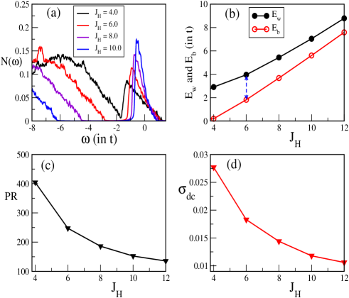
Figure 1: Shows the (a) density of states $N(\omega)$ with the formation of IB for different values of the Hund’s coupling $J_{H}$. Fermi energy is set at zero; (b) change in the binding energy $E_{b}$ and the $E_{w}$ with $J_{H}$ showing the localization-induced narrowing of the IB (the double arrow shows the width of the IB for $J_{H}$ = 6); (c) variation of the participation ratio with $J_{H}$ distinguishing the extended states from the localized states, and (d) decrease in the dc conductivity (in units of ${\pi e^{2}}/{\hbar a}$) with $J_{H}$ indicating carrier localization as in (c). All calculations are made at fixed impurity concentration $x$ = 0.25, carrier concentration $p$ = 0.2, and temperature $T$ = 0.05.

III Formation of the impurity band

The nature of the IB plays the key role in determining the ferromagnetic state which solely depends on the exchange interaction $J_{H}$ and the amount of the magnetic impurities $x$ in the system. Ultra-fast transient reflectivity spectra ishii and magnetic circular dichroism measurements dobrowolska show the existence of a preformed IB inside the bandgap of in GaMnAs. We start our calculation for $x$ = 0.25, where a separated IB starts to form for $J_{H}$ = 4 even at relatively high temperature $T$ = 0.05 as shown in the density of states (DOS) $N(\omega)=\langle{1\over N}\sum_{\alpha}\delta(\omega-\epsilon_{\alpha})\rangle$ in Fig. 1(a). Here the binding energy $E_{b}$ = (bottom of the IB - top of the VB) $\sim$0.2$t$, where the small finite density of states between the VB and the IB is due to the broadening used to calculate the DOS. We define the quantity $E_{w}$ (= top of the IB - top of the VB), which must be smaller than the bandgap of the host semiconductor. So $E_{w}$ - $E_{b}$ is the width of the impurity band. With increase in the local Hund’s coupling the carriers get localized at the impurity sites, consequently the IB becomes narrower and also moves away from the VB as evident from Fig. 1(b). From these results next we fix the $J_{H}$ values to mimic GaMnAs and GaMnN like systems.

GaMnAs is a low bandgap ($\sim$ 1.5 eV) system with long-ranged ferromagnetic interaction where the $E_{b}$ is only about $\sim$ 0.1 eV. Hence we choose $J_{H}$ = 4 for GaMnAs for which $E_{b}$ $\sim$ 0.1 eV (0.2t) and $E_{w}$ is $\sim$ 1.5 eV (3$t$). Direct measurements yield $J_{H}$ = 1.2 eV - 3.3 eV [7; 8; 6] for GaMnAs. Note that we absorbed the impurity spin magnitude 5/2 into $J_{H}$ which scales with $t$ (= 0.5 eV). So our $J_{H}$ value is in the range as reported in experiments. In contrast, the bandgap of GaMnN is $\sim$ 3.4 eV. And, the IB is distinctly separated from the VB located at an energy $\sim$ 1.5 eV ($E_{b}$) above the VB implying the short-range character of the ferromagnetic interactions. So in this case we choose $J_{H}$ = 10, where $E_{b}$ $\sim$ 2.75 eV and $E_{w}$ is $\sim$ 3.5 eV (7$t$). Later, we will see that the NNN hopping $t^{\prime}$ hardly alter the $E_{w}$ value but significantly affects the ferromagnetic state.

The degree of structural or magnetic disorder is inversely proportional to the participation ratio PR $=1/\sum_{i}(\psi_{l}^{i})^{4}$, where $\{\psi_{l}\}$ are the quasiparticle wave functions. PR together with the DOS provide an extensive picture of both spectral and spatial features of quasiparticle states. The participation ratio provides a measure of the number of lattice sites over which the state is extended. For normalized wave functions the PR can range between $N$ for a fully extended state and 1 for a site-localized state. In Fig. 1(c) we plot the PR of the state at the Fermi energy ($E_{F}$) with $J_{H}$ at fixed $p$ = 0.2 and T = 0.05. For the chosen Hund’s couplings $J_{H}$ = 4 and 10 the states are extended over $\sim$ 400 sites and only over $\sim$ 150 sites, respectively. It reflects the fact that the long- and the short-range nature of the exchange interactions in GaMnAs and GaMnN like systems are automatically accounted in the calculations.

Then we calculate the dc conductivity by using the Kubo-Greenwood formula mahan-book ; cond-ref

$$\sigma(\omega)={A\over N}\sum_{\alpha,\beta}(n_{\alpha}-n_{\beta}){{|f_{\alpha\beta}|^{2}}\over{\epsilon_{\beta}-\epsilon_{\alpha}}}\delta(\omega-(\epsilon_{\beta}-\epsilon_{\alpha}))$$ (1)

with $A={\pi e^{2}}/{{\hbar a}}$, where $a$ is the lattice spacing. $n_{\alpha}(Fermifactors)=f(\mu-\epsilon_{\alpha})$ and $\epsilon_{\alpha}$, $\epsilon_{\beta}$ are the corresponding eigen energies. And, $f_{\alpha\beta}$=$\langle\psi_{\alpha}|$$j_{x}$$|\psi_{\beta}\rangle$ are the matrix elements of the current operator $j_{x}=it\sum_{i,\sigma}(c^{\dagger}_{{i+x},\sigma}c_{i,\sigma}-h.c.)$. Finally, the dc conductivity is obtained by averaging the conductivity over a small low frequency interval $\Delta\omega$ defined as

$$\sigma_{av}(\Delta\omega)={1\over{\Delta\omega}}\int_{0}^{\Delta\omega}\sigma(\omega){\rm d}\omega.$$

$\Delta\omega$ is chosen three to four times larger than the mean finite-size gap of the system (determined by the ratio of the bare bandwidth and the total number of eigenvalues). This procedure has been benchmarked in a previous work cond-ref . The conductivity for fixed $p$ =0.2 at $T$ = 0.05 is shown in Fig. 1(d). The decrease in conductivity with $J_{H}$ substantiates the fact that the carriers get localized with Hund’s coupling as seen in Fig. 1(a)-(c).

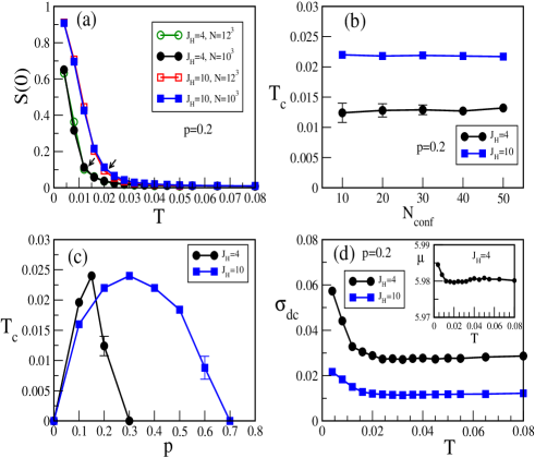
Figure 2: Displays various physical quantities for $J_{H}$ = 4 and 10 at fixed $x$=0.25. In case of fixed carrier density calculations, $p$=0.2. It demonstrates the (a) ferromagnetic structure factor S(0) for two system sizes 10³ and 12³, which are almost indistinguishable. The arrows point the $T_{C}$ values; (b) $T_{C}$ with error vs the number of configurations $N_{conf}$ clarifying that $N_{conf}$ = 10 is reasonably good for our qualitative investigations; (c) ferromagnetic windows $T_{C}$ vs $p$ showing the localization induced widening of the FM window in case of $J_{H}$=10, and (d) dc conductivity vs temperature illustrating the more metallicity of the long-range interacting systems ($J_{H}$=4) compared to the short-range interacting systems ($J_{H}$=10). The inset shows the variation of chemical potential $\mu$ with temperature for $J_{H}$=4, required to set the desired $p$ = 0.2.

IV Ferromagnetic Windows for $t^{\prime}$ = 0

In order to see the effects of localization on ferromagnetism we estimate the $T_{C}$ from the ferromagnetic structure factor $S(\textbf{0})$, where $S(\textbf{q})$ =${1\over N}$ $\sum_{ij}$ $\bf{\bf S}_{i}\cdot{\bf S}_{j}$ e${}^{i\bf{q}\cdot({\bf r}_{i}-{\bf r}_{j})}$ (q are the wave vectors). The average structure factors for $J_{H}$=4 and 10 are shown in Fig. 2(a) for $p$=0.2 using system sizes $10^{3}$ and $12^{3}$. As the data of these two system sizes are barely distinguishable from each other, so we use $N=10^{3}$ for all calculations in this work. We estimate $T_{C}$ from each structure factor and then average it over ten different configurations, which is sufficient enough as shown in Fig. 2(b). $T_{C}$ value remains more or less same with the number of configurations $N_{conf}$. The error for $J_{H}$=4 and $p$=0.2 is found to decrease with the number of configurations and is in the acceptable range for $N_{conf}$=10 for our qualitative investigations. And, for $J_{H}$=10 and $p$=0.2 the error is insignificant i.e. the error bars are smaller than point sizes for all different $N_{conf}$ we considered.

Next we plot the ferromagnetic windows for $J_{H}$=4 and 10 in Fig. 2(c). The range of the FM window for $J_{H}$=4 is from $p$=0 to 0.3. In the higher hole density regime the carriers hopping gets restricted due to large delocalization length, and as a result kinetic energy is minimized and hence the $T_{C}$ is suppressed. On the other hand carriers are less extended for $J_{H}$=10 [see Fig. 1]. Consequently, the carrier hopping is stimulated to gain kinetic energy resulting in wider FM window. In addition, in Fig. 2(d) we plot the dc conductivity in a wide range of temperature to corroborate the fact that the carriers are relatively more localized for $J_{H}$=10 as compared to $J_{H}$=4. All calculations with temperature are carried out for fixed carrier density $p$. The standard procedure to set the desired $p$ at all temperatures is by varying the chemical potential $\mu$ accordingly with temperature as shown for $J_{H}$=4 and $p$=0.2 in the inset.

The nature of the carriers that mediate the ferromagnetism and in turn controls the $T_{C}$ depends upon the location of the IB relative to the VB. Where, for $J_{H}$ = 4 (GaMnAs-like) the gap is very small, that for $J_{H}$ = 10 (GaMnN-like) is large, clearly displaying a separated IB (see Fig. 1). Keeping aside the GaMnN case, in literature there are two conflicting theoretical viewpoints on the nature of the carriers in GaMnAs. In one of those extreme limits the IB is very much boardened and indistinguishable from valence band, known as the VB picture. In this approach within the mean-field Zener model, the magnetic impurities induce itinerant carriers in the VB of the host materials, which mediate the long-range magnetic interactions dietl ; jungwirth1 . It has been generally accepted because of it’s ability to explain a variety of features of GaMnAs dietl ; dietl2 ; dietl3 ; jungwirth ; jungwirth1 ; neumaier ; nishitani ; marco ; tesarova ; sawicki . The key prediction of this approach is that $T_{C}$ increases monotonically with both the effective Mn concentration and the carrier density jungwirth1 . However, this model is contradicted by electronic structure calculations tang ; zunger ; sanvito1 and argued that ferromagnetism in GaMnAs is determined by impurity-derived states that are localized. This is commonly known as the IB picture. Several experiments on the optical hirakawa ; burch ; sapega ; ando1 and transport rokhinson ; alberi properties have reported that $E_{F}$ exists in the IB within the bandgap of GaMnAs. Results from resonant tunneling also suggests that the VB remains nearly non-magnetic in ferromagnetic GaMnAs and does not merge with the IB ohya . This picture successfully explains the nonmonotonic variation of $T_{C}$ with $p$ observed in Refs. [36; 37]. This is in clear disagreement with the prediction of the valence band picture dietl ; jungwirth1 . However, recently it was also suggested that both the mechanisms can be active simultaneously in GaMnAs sato . In spite of all efforts the issue of IB picture versus VB picture is still inconclusive.

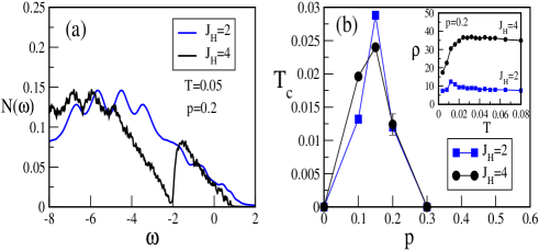
Figure 3: Shows the (a) density of states $N(\omega)$ for $J_{H}$ = 2 and 4 at fixed $p$=0.2 and T=0.05. Fermi energy is set at zero. There is no signature of IB for $J_{H}$ = 2, and (b) ferromagnetic windows $T_{C}$ vs $p$ for $J_{H}$ = 2 and 4. Inset plots the resistivity (in units of ${\hbar a}/{\pi e^{2}}$) Vs temperature, at $p$=0.2, indicating more metallicity in case of $J_{H}$ = 2. We fixed $x=0.25$ for these calculations.

In this battle of bands samarth where do our assumption of IB picture for $J_{H}$ = 4 in Fig. 1 stands? As we have considered $x$ = $25\%$ in a N = $10^{3}$ system, in the ideal situation the IB picture can be assigned when the participation ratio is within 250 i.e. the carriers are located only at the magnetic sites. DOS along with PR in Fig. 1 reveal that for higher values of $J_{H}$ (=6 or more) the carriers are restricted to the magnetic sites [see Fig. 1(c)] and so can be categorized in the IB model. But, in case of $J_{H}$ = 4 the IB is very close to the VB and so there is significant probability of hopping of the holes from the magnetic to host sites. In fact, due to this hopping process, the participation ratio for $J_{H}$ = 4 [see Fig. 1(c)] is $\sim$400. This shows that there is significant mixing between the VB and IB. Interestingly, even in the mixed nature of the carriers in case of $J_{H}$ = 4 the $T_{C}$ varies non-monotonically unlike in the valence band picture jungwirth1 . So there is a natural curiosity to check the $T_{C}$ trend in the pure VB picture in our calculation. For this we consider the lower Hund’s coupling $J_{H}$ = 2. The DOS plotted in Fig. 3(a) shows that there is no signature of IB at all. Also, the calculated PR of the Fermi state for $p$ =0.2 is $\sim$800. Clearly, this comes in the category of VB picture with more metallicity compared to moderately and strongly coupled systems (see the inset of Fig. 3(b)). Most interestingly, the $T_{C}$ shows an optimization behavior with respect to $p$ as in the case of $J_{H}$ = 4 [see Fig. 3(b)]. So we found that the non-monotonic behavior of $T_{C}$ is independent of the VB and the IB pictures. Similar results also found by other techniques such as spin wave and earlier MC calculations singh ; singh1 ; alvarez ; bui .

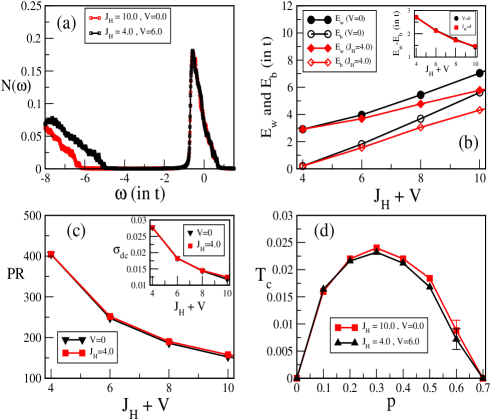
Figure 4: Presents the comparison of various physical quantities between the $t-J_{H}$ and the $t-J_{H}-V$ models at fixed $x$ = 0.25. It compares the (a) density of states $N(\omega)$ for two sets of parameters ($J_{H},V$)=(4,6) and (10,0), where features of the IBs are shown to match completely. Fermi energy is set at zero; (b) variation of the binding energy $E_{b}$ and the $E_{w}$ for different sets of ($J_{H},V$) values. In the x-axis $J_{H}+V$ is varied in two different ways: (i) by varying $V$ with fixed $J_{H}$=4 and (ii) by varying $J_{H}$ with fixed $V$=0. Second one is the $t-J_{H}$ model for which the physical quantities are replotted from Fig 1. This shows that although $E_{b}$ and $E_{w}$ differ from one representation to other but the width of the IBs match well in the whole parameter range [see the inset]; (c) variation of the participation ratio and the dc conductivity (in units of ${\pi e^{2}}/{\hbar a}$) [in the inset] with ($J_{H}+V$) values as in (b). There is one-to-one correspondence between them, and (d) ferromagnetic windows $T_{C}$ vs $p$ showing a good match for the two sets of parameters as in (a). In (a)-(c) the calculations are carried out at fixed $p$ = 0.2 and $T$ = 0.05.

V Correspondence between $t-J_{H}$ and $t-J_{H}-V$ Models

The properties of the IB and hence the ferromagnetic window can be tuned by varying the binding energy of the carriers. Hence it is worthful to highlight the $t-J_{H}-V$ model at this point before proceeding with the NNN hopping term in the Hamiltonian. Here the potential term is represented by $\sum_{m}V_{m}n_{m}$ with $V_{m}$=V at impurity sites and 0 otherwise. Apart from the magnetic nature of the Hund’s term both $J_{H}$ and $V$ act as the trapping centers for the carriers at the impurity sites. So it would be interesting to check whether the $t-J_{H}-V$ model can be qualitatively replaced by a only $t-J_{H}$ model or not, in the parameter regime we consider. We benchmark our results by comparing these two models. Fig. 4(a) shows the DOSs for ($J_{H},V$) = (10, 0) and (4, 6), where the IB is seen to be unaffected. Fig. 4(b) presents the binding energy $E_{b}$ and the $E_{w}$ for different sets of ($J_{H},V$) values. In the x-axis $J_{H}+V$ is defined in two different ways; (i) by varying V with fixed $J_{H}$ = 4 representing the $t-V-J_{H}$ model and (ii) by varying $J_{H}$ with fixed V = 0 representing the $t-J_{H}$ model. Although the $E_{w}$ and the $E_{b}$ differ from one representation to other for the whole parameter range the widths of the IBs match well [see the inset]. Consequently, the PR and the conductivity results (see Fig. 4(c) and it’s inset) for $t-J_{H}-V$ model is more or less same to $t-J_{H}$ model. The comparison of the ferromagnetic windows for both the set of parameters ($J_{H},V$)= (10, 0) and (4, 6) indicate that the $t-J_{H}-V$ model can be qualitatively replaced with a suitable choice of $t-J_{H}$ only, shown in Fig. 4(d). Therefore for simplicity we specifically explore the $t-J_{H}$ model for our further investigations.

VI Effects of next nearest neighbor hopping for $J_{H}$=4

In the recent past Dobrowolska et al.[36] demonstrated the existence of a preformed IB in GaMnAs and the $T_{C}$ is decided by the location of the Fermi energy within the impurity band. In this picture the states at the center of the impurity band are extended resulting in maximum $T_{C}$. And, the $T_{C}$ gets reduced towards both the top and the bottom ends of the band due to localized states. In the process insulator-metal-insulator (I-M-I) transition is observed with carrier density. Most importantly, they observed the ferromagnetic state in a wide range of hole density $p$ $\sim$ 0.1-0.9. In Fig. 2(c) our FM window ranges only from $p$ = 0 to 0.3 for $J_{H}$ = 4. So now we are going to investigate this mismatch by taking the impact of NNN hopping on the carrier mobility and magnetic properties into account.

We start with the comparison of the spin-resolved density of states for $t^{\prime}$ = 0 and 0.2 at fixed $p$ = 0.2 and T = 0.004 [see Fig. 5(a)] for which ground states are ferromagnetic. In both the cases the impurity band is spin polarized, while the VB remains more or less unpolarized. In our hole picture positive $t^{\prime}$ acts as a localizing agent which can be visualized from the DOS, where the IB becomes narrow and shifts away from the VB. This is also apparently clear from the PR shown in Fig. 5(b), where the quasiparticle states in case of $t^{\prime}$=0.2 are localized compared to $t^{\prime}$=0 in the whole range of p. It is also important to note that $t^{\prime}$ doesn’t alter the value of $E_{w}$ ($\sim$ 3$t$) which is well within the bandgap of the host. Alternatively, higher $J_{H}$ can also localize the carriers (as shown in Fig. 1(a)) and ultimately boarden the FM window (see Fig 2(c)), but $E_{w}$ becomes larger [see Fig. 1(b)] than the bandgap which is not physically acceptable for narrow bandgap host like GaAs.

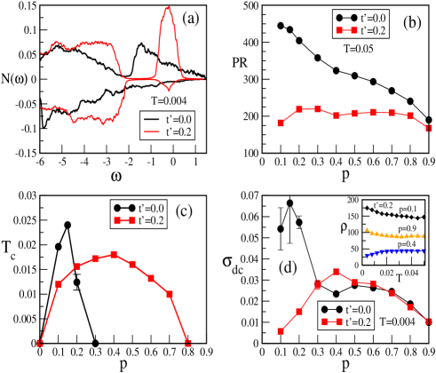
Figure 5: The effects of the next-nearest-neighbor hopping ($t^{\prime}$ = +0.2) and it’s comparison to $t^{\prime}$ = 0 are shown for various physical quantities at fixed $J_{H}$ = 4 and $x$ = 0.25. It presents the (a) spin-resolved density of states at fixed $T$ = 0.004, where the IB shrinks and moves away from the VB due to carrier localization. The Fermi energy is set at zero; (b) change in the participation ratio (PR) with $p$ at fixed $T$ = 0.05 showing the higher degree of localization for $t^{\prime}$ = +0.2; (c) displays the $t^{\prime}$-induced broadening of the ferromagnetic window $T_{C}$ vs $p$, and (d) dc conductivities (in units of ${\pi e^{2}}/{\hbar a}$) with $p$ at fixed $T$ = 0.004. I-M-I is confirmed from the resistivity (in units of ${\hbar a}/{\pi e^{2}}$) Vs temperature plot for different carrier densities, in the inset. The localization driven I-M-I transition is consistent with the results presented in (c).

We present the ferromagnetic window, $T_{C}$ vs $p$, for GaMnAs in Fig. 5(c). The $T_{C}$ optimizes around $p$=0.15 and the ferromagnetism is restricted to a small window of $p$ = 0-0.3 for $t^{\prime}$=0. At higher hole concentration the carrier mobility is suppressed due to larger delocalization length in GaMnAs, see Fig. 5(b). One can remobilize the carriers by reducing their overlap with a mild localization of the carriers which is stimulated by the NNN hopping parameter $t^{\prime}$ = 0.2 as shown in Fig. 5(b). Consequently, the ferromagnetism is activated and the window [see Fig. 5(c)] becomes wider ($p$ = 0-0.8) as observed in the experiments ($p$ $\sim$ 0.1-0.9) [36; 30]. In order to correlate the magnetic and transport properties we plot the low temperature ($T$ = 0.004) dc conductivity in Fig. 5(d). In a carrier-mediated magnetic system a minimum amount of carrier is necessary to initiate the magnetic interactions, and at higher $p$ the magnetism is suppressed due to the decrease in carrier mobility. Hence in these regimes the system is insulating and in intermediate $p$ the system is metallic resulting in higher $T_{C}$. For both $t^{\prime}$ = 0 and 0.2 conductivity goes through IMI transition with optimization around the same value of $p$ as in case of $T_{C}$ vs $p$ window, which supports the above carrier localization picture and also qualitatively matches with the experiment dobrowolska . Resistivity vs Temperature plot in the inset of Fig. 5(d) explicitly shows the IMI transition as we increase the hole density. Experimental data together with our findings hint the presence of NNN-hopping in GaMnAs like systems. But further probe and investigations are necessary to establish this scenario.

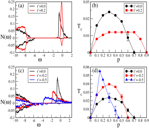
Figure 6: The effects of the $t^{\prime}$ = +0.2 and it’s comparison to $t^{\prime}$ = 0 are presented for (a) the spin-resolved density of states at fixed $T$ = 0.004, where the IB moves away from the VB due to carrier localization and (b) the ferromagnetic window $T_{C}$ vs $p$ showing the localization-induced broadening. The effects of the $t^{\prime}$ =-0.2 and -0.5 with it’s comparison to $t^{\prime}$ = 0 are presented for (c) the spin-resolved density of states at fixed $T$ = 0.004, where the IB extended towards the VB due to carrier delocalization, and (d) the ferromagnetic windows showing the delocalization-induced shrinkening. The Fermi energy is set at zero. We fixed $J_{H}$ = 10 and $x=0.25$ for all calculations.

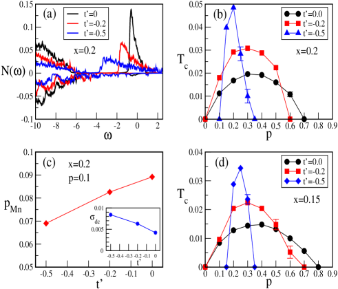
Figure 7: The effects of the $t^{\prime}$ = -0.2 and -0.5 with it’s comparison to $t^{\prime}$ = 0 at fixed $x$ = 0.2 are shown for (a) the spin-resolved density of states at fixed $T$ = 0.004 and (b) the ferromagnetic windows $T_{C}$ vs $p$. For higher degree of delocalization the FM window becomes significantly narrow. (c) plots the average carrier density per magnetic impurity site ($p_{Mn}$) vs $t^{\prime}$ at fixed $p$=0.1 and $T$ = 0.05, which reveals the out flow of carriers to non-magnetic sites with delocalization. In consequence the overall conductivity of the system increases as shown in the inset. We find similar narrowing of FM window for $x$ = 0.15 and presented in (d). We considered $J_{H}$ = 10 for all calculations.

VII Effects of next nearest neighbor hopping for $J_{H}$=10

Now we study the GaMnN with the chosen Hund’s coupling $J_{H}$ = 10. The spin-resolved DOS and the FM windows are evaluated with the same set of parameter values as in Fig. 5. Fig. 6(a) and (b) show that the effect of NNN hopping on the IB and FM window are qualitatively similar as in the case of $J_{H}$ = 4. Quantitatively, the effect of localization due to $t^{\prime}$ is much more prominent for $J_{H}$ = 10 and as a result the deduction of $T_{C}$ is significant. But, the electronic structure calculations reveal that the Ga defects in GaMnN introduce states between the VB and the IB which depopulate the IB and in turn destroy the ferromagnetism in GaMnN mahadevan . We mimic the situation by introducing negative NNN hopping which delocalize the carriers and consequently broaden the IB towards the VB. This can be seen from the DOS plotted in Fig. 6(c) for $t^{\prime}$ = -0.2 and -0.5 along with $t^{\prime}$ = 0 at fixed $p$ = 0.2 and $T$ = 0.004. Note that the binding energy $E_{b}$ decreases but $E_{w}$ remains more or less unaffected (i.e. $E_{w}$ is within the bandgap of host GaMnN). As positive and negative $t^{\prime}$ play opposite roles in the system, so the ferromagnetic window shrinks and the optimum $T_{C}$ increases with carrier delocalization, as shown in Fig. 6(d).

The solubility of Mn in GaAs and GaN is low, so we establish our findings by calculating the ferromagnetic windows for lower impurity concentrations. First we consider $x$ = 0.2 and the results for the spin-resolved DOS and the FM windows are presented in Fig. 7(a) and (b) respectively. The IBs show qualitatively similar evolution with $t^{\prime}$ as in case of $x$ = 0.25. Apart from the disappearance of ferromagnetism in the higher $p$ regime, interestingly, the magnetism also vanishes for very low carrier densities for $t^{\prime}$= -0.5 making the FM window furthermore narrow. Note that we have considered the relative carrier density i.e. number of carrier per Mn impurity site as in experiments. So, in the low $x$ and lower $p$ regime the magnetic sites accumulate a tiny amount of holes resulting in a weaker magnetic interactions. Here, if we increase the carrier mobility the holes get deplete from the magnetic to the non-magnetic sites which further suppresses the spin-spin couplings. The out flow of carriers is displayed in Fig. 7(c) where we plot the average carrier density at the magnetic sites $p_{Mn}$ vs $t^{\prime}$ at fixed $p$=0.1. Eventually, the ferromagnetism vanishes at lower $p$ as in case of $t^{\prime}$ = -0.5. On the other hand, the overall conductivity of the system increases with the degree of delocalization as shown in the inset. We find similar results for $x$ = 0.15 [Fig. 7(d)]. The vanishing ferromagnetism in both lower and higher $p$ regimes for $t^{\prime}$ = -0.5 makes the ferromagnetic window significantly narrow, which suppresses the probability of getting a FM state. In experiments the presence of defects makes the sample preparation very crucial and our results indicate that unless the system has a favourable combination of $x$ and $p$ in a narrow window then there is a higher chance to observe either low $T_{C}$ or absence of ferromagnetism. In addition, the sharp increase in the optimum $T_{C}$ in a thin window of $p$ clarifies the room temperature ferromagnetism occasionally observed in experiments.

VIII Conclusions

In conclusion, we investigated the magnetic and the transport properties of III-V DMSs using a classical Monte-Carlo method within the $t-t^{\prime}$ Kondo lattice model on a simple cubic lattice. We have shown that the carrier mobility induced by the NNN hopping $t^{\prime}$ plays a vital role in determining the ferromagnetic states in both GaMnAs and GaMnN like systems. In case of GaMnAs a small positive $t^{\prime}$ (that helps to localize the carriers) is shown to be necessary to reproduce the robustness of the ferromagnetic states in a wide range of carrier concentration as observed in experiments. On the other hand, if we delocalize the carriers by activating negative $t$’ the ferromagnetic window significantly shrinks with an enhancement of the optimum value of $T_{C}$ in GaMnN. We correlate our findings with the experimental results and suggest that Ga like vacancy in GaMnN that depopulate the IB triggers high $T_{C}$ in low hole density. In reality, the presence of intrinsic defects is inevitable and also the carrier density is not controllable. So the probability of having an optimal amount of holes in a narrow regime in Ga defected GaMnN is very low. This could be the reason of occasional appearance of ferromagnetism and in turn keeps the high $T_{C}$ issue of GaMnN unresolved till date.

Acknowledgment: We acknowledge use of Meghnad2019 computer cluster at SINP.

References

- (1) H. Munekata, H. Ohno, S. von Molnar, Armin Segmueller, L. L. Chang, and L. Esaki, Phys. Rev. Lett. 63, 1849 (1989).
- (2) H. Ohno, Science 281, 951 (1998).
- (3) T. Jungwirth, Jairo Sinova, J. Masek, J. Kucera, and A. H. MacDonald, Rev. Mod. Phys. 78, 809 (2006).
- (4) T. Dietl and H. Ohno, Rev. Mod. Phys. 86, 187 (2014).
- (5) H. Ohno, A. Shen, F. Matsukura, A. Oiwa, A. Endo, S. Katsumoto, and Y. Iye, Appl. Phys. Lett. 69, 363 (1996).
- (6) F. Matsukura, H. Ohno, A. Shen, and Y. Sugawara, Phys. Rev. B 57, R2037(R) (1998).
- (7) J. Okabayashi, A. Kimura, O. Rader, T. Mizokawa, A. Fujimori, T. Hayashi, and M. Tanaka. Phys. Rev. B 58, R4211(R) (1998).
- (8) K. Ando, T. Hayashi, M. Tanaka, and A. Twardowski, J. Appl. Phys. 83, 6548 (1998).
- (9) T. Dietl, H. Ohno, F. Matsukura, J. Cibert, and D. Ferrand, Science 287, 1019 (2000).
- (10) T. Jungwirth, K. Y. Wang, J. Masek, K. W. Edmonds, J. Koenig, J. Sinova, M. Polini, N. A. Goncharuk, A. H. MacDonald, M. Sawicki, A. W. Rushforth, R. P. Campion, L. X. Zhao, C. T. Foxon, and B. L. Gallagher, Phys. Rev. B 72, 165204 (2005).
- (11) L. Chen, X. Yang, F. Yang, J. Zhao, J. Misuraca, P. Xiong, and S. von Molnar, Nano Lett. 11, 2584 (2011).
- (12) L. Chen, S. Yan, P. F. Xu, J. Lu, W. Z. Wang, J. J. Deng, X. Qian, Y. Ji, and J. H. Zhao, Appl. Phys. Lett. 95, 182505 (2009).
- (13) S. Sonoda, S. Shimizu, T. Sasaki, Y. Yamamoto, and H. Hori, J. Cryst. Growth 237-239, 1358 (2002).
- (14) M. L. Reed, N. A. El-Masry, H. H. Stadelmaier, M. K. Ritums, M. J. Reed, C. A. Parker, J. C. Roberts, and S. M. Bedair, Appl. Phys. Lett. 79, 3473 (2001).
- (15) G. T. Thaler, M. E. Overberg, B. Gila, R. Frazier, C. R. Abernathy, S. J. Pearton, J. S. Lee, S. Y. Lee, Y. D. Park, Z. G. Khim, J. Kim and F. Ren, Appl. Phys. Lett. 80, 3964 (2002).
- (16) L. Kronik, M. Jain, and J. R. Chelikowsky, Phys. Rev. B 66, 041203(R) (2002).
- (17) K. Sato, L. Bergqvist, J. Kudrnovsky, P. H. Dederichs, O. Eriksson, I. Turek, B. Sanyal, G. Bouzerar, H. Katayama-Yoshida, V. A. Dinh, T. Fukushima, H. Kizaki, and R. Zeller, Rev. Mod. Phys. 82, 1633 (2010).
- (18) T. Dietl, Nat. Mat. 9, 965 (2010).
- (19) R. Q. Wu, G. W. Peng, L. Liu, Y. P. Feng, Z. G. Huang, and Q. Y. Wu, App. Phys. Lett. 89, 142501 (2006).
- (20) X. Peng and R. Ahuja, App. Phys. Lett. 94, 102504 (2009).
- (21) S. W. Fan, K. L. Yao, Z. L. Liu, G. Y. Gao, Y. Min, and H. G. Cheng, J. App. Phys. 104, 043912 (2008).
- (22) P. Dev and P. Zhang, Phys. Rev. B 81, 085207 (2010).
- (23) P. Dev, Y. Xue, and P. Zhang, Phys. Rev. Lett. 100, 117204 (2008).
- (24) P. Larson and S. Satpathy, Phys. Rev. B 76, 245205 (2007).
- (25) J. Missaoui, I. Hamdi, and N. Meskini, J. Magn. Magn. Mater. 413, 19 (2016).
- (26) J. Osorio-Guillen, S. Lany, S. V. Barabash, and A. Zunger, Phys. Rev. Lett. 96, 107203 (2006).
- (27) E. Kan, Fang Wu, Y. Zhang, H. Xiang, R. Lu, C. Xiao, K. Deng, and H. Su, Appl. Phys. Lett. 100, 072401 (2012).
- (28) R. C. Myers, B. L. Sheu, A. W. Jackson, A. C. Gossard, P. Schiffer, N. Samarth, and D. D. Awschalom, Phys. Rev. B 74, 155203 (2006).
- (29) K. M. Yu, W. Walukiewicz, T. Wojtowicz, I. Kuryliszyn, X. Liu, Y. Sasaki, and J. K. Furdyna, Phys. Rev. B 65, 201303(R) (2002).
- (30) Y. J. Cho, K. M. Yu, X. Liu, W. Walukiewicz, and J. K. Furdyna, Appl. Phys. Lett. 93, 262505 (2008).
- (31) S. J. Potashnik, K. C. Ku, S. H. Chun, J. J. Berry, N. Samarth, and P. Schiffer, Appl. Phys. Lett. 79, 1495 (2001).
- (32) J. Szczytko, W. Mac, A. Twardowski, F. Matsukura, and H. Ohno, Phys. Rev. B 59, 12935 (1999).
- (33) M. Jain, L. Kronik, J. R. Chelikowsky, and V. V. Godlevsky, Phys. Rev. B 64, 245205 (2001).
- (34) M. Wierzbowska, D. Sanchez-Portal, and S. Sanvito Phys. Rev. B 70, 235209 (2004).
- (35) B. Sanyal, O. Bengone, and S. Mirbt, Phys. Rev. B 68, 205210 (2003).
- (36) M. Dobrowolska, K. Tivakornsasithorn, X. Liu, J. K. Furdyna, M. Berciu, K. M. Yu, and W. Walukiewicz, Nat. Mat. 11, 444 (2012).
- (37) B. C. Chapler, S. Mack, R. C. Myers, A. Frenzel, B. C. Pursley, K. S. Burch, A. M. Dattelbaum, N. Samarth, D. D. Awschalom, and D. N. Basov, Phys. Rev. B 87, 205314 (2013).
- (38) K. M. Yu, W. Walukiewicz, T. Wojtowicz, J. Denlinger, M. A. Scarpulla, X. Liu, and J. K. Furdyna, Appl. Phys. Lett. 86, 042102 (2005).
- (39) V. Novak, K. Olejnik, J. Wunderlich, M. Cukr, K. Vyborny, A. W. Rushforth, K. W. Edmonds, R. P. Campion, B. L. Gallagher, Jairo Sinova, and T. Jungwirth, Phys. Rev. Lett. 101, 077201 (2008).
- (40) M. Wang, R. P. Campion, A. W. Rushfortha, K. W. Edmonds, C. T. Foxon, and B. L. Gallagher, Appl. Phys. Lett. 93, 132103 (2008).
- (41) K. C. Ku, S. J. Potashnik, R. F. Wang, S. H. Chun, P. Schiffer, N. Samarth, M. J. Seong, A. Mascarenhas, E. Johnston-Halperin, R. C. Myers, A. C. Gossard, and D. D. Awschalom, Appl. Phys. Lett. 82, 2302 (2003).
- (42) E. Sarigiannidou, F. Wilhelm, E. Monroy, R. M. Galera, E. Bellet-Amalric, A. Rogalev, J. Goulon, J. Cibert, and H. Mariette, Phys. Rev. B 74, 041306(R) (2006).
- (43) M. E. Overberg, C. R. Abernathy, S. J. Pearton, N. A. Theodoropoulou, K. T. McCarthy, and A. F. Hebard, Appl. Phys. Lett. 79, 1312 (2001).
- (44) Y. L. Soo, G. Kioseoglou, S. Kim, S. Huang, Y. H. Kao, S. Kuwabara, S. Owa, T. Kondo, and H. Munekata, Appl. Phys. Lett. 79, 3926 (2001).
- (45) P. Mahadevan and A. Zunger, Appl. Phys. Lett. 85, 2860 (2004).
- (46) T. Graf, M. Gjukic, M. S. Brandt, M. Stutzmann, and O. Ambacher, Appl. Phys. Lett. 81, 5159 (2002).
- (47) L. Janicki, G. Kunert, M. Sawicki, E. Piskorska-Hommel, K. Gas, R. Jakiela, D. Hommel, and R. Kudrawiec, Scientific Reports 7, 41877 (2017).
- (48) R. Bouzerar and G. Bouzerar, Europhys. Lett. 92, 47006 (2010).
- (49) R.Y. Korotkov, J. M. Gregie, and B. W. Wessels, Appl. Phys. Lett. 80, 1731 (2002).
- (50) K. H. Kim, K. J. Lee, D. J. Kim, H. J. Kim, and Y. E. Ihm, C. G. Kim, S. H. Yoo and C. S. Kim, Appl. Phys. Lett. 82, 4755 (2003).
- (51) P. Mahadevan and S. Mahalakshmi, Phys. Rev. B 73, 153201 (2006).
- (52) S Sonoda, I. Tanaka, H. Ikeno, T. Yamamoto, F. Oba, T. Araki, Y. Yamamoto, K. Suga, Y. Nanishi, Y. Akasaka, K. Kindo and H. Hori, J. Phys.: Condens. Matter 18, 4615 (2006).
- (53) S. Limpijumnong and C. G. Van de Walle, Phys. Rev. B 69, 035207 (2004).
- (54) S. Kumar and P. Majumdar, Eur. Phys. J. B 50, 571 (2006).
- (55) G.Alvarez, M. Mayr, and E. Dagotto, Phys. Rev. Lett. 89, 277202 (2002).
- (56) A. Chattopadhyay, S. Das Sarma, and A. J. Millis, Phys. Rev. Lett. 87 227202 (2001).
- (57) Mona Berciu and R. N. Bhatt, Phys. Rev. Lett. 87, 107203 (2001).
- (58) K. Pradhan and P. Majumdar, Euro. Phys. Lett. 85, 37007 (2009).
- (59) A. Singh, S. K. Das, A. Sharma, and A. Nolting, J. Phys.: Condens. Matter 19, 236213 (2007).
- (60) K. Pradhan and S. K. Das, Scientific Reports 7, 9603 (2017).
- (61) T. Ishii, T. Kawazoe, Y. Hashimoto, H. Terada, I. Muneta, M. Ohtsu, M. Tanaka, and S. Ohya, Phys. Rev. B 93, 241303(R) (2016).
- (62) G. D. Mahan, Quantum Many Particle Physics (Plenum Press, New York, 1990).
- (63) S. Kumar and P. Majumdar, Europhys. Lett. 65, 75 (2004).
- (64) T. Dietl, H. Ohno and Matsukura, Phys. Rev. B 63, 195205 (2001).
- (65) D. Neumaier, M. Turek, U. Wurstbauer, A. Vogl, M. Utz, W. Wegscheider, and D. Weiss, Phys. Rev. Lett. 103, 087203 (2009).
- (66) Y. Nishitani, D. Chiba, M. Endo, M. Sawicki, F. Matsukura, T. Dietl, and H. Ohno, Phys. Rev. B 81, 045208 (2010).
- (67) I. Di Marco, P. Thunstrom, M. I. Katsnelson, J. Sadowski, K. Karlsson, S. Leeegue, J. Kanskan and O. Eriksson, Nat. Comm. 4, 2645 (2013).
- (68) N. Tesarova, T. Ostatnicky, V. Novak, K. Olejnik, J. Subrt, H. Reichlova, C. T. Ellis, A. Mukherjee, J. Lee, G. M. Sipahi, J. Sinova, J. Hamrle, T. Jungwirth, P. Nemec, J. Cerne, and K. Vyborny, Phys. Rev. B 89, 085203 (2014).
- (69) M. Sawicki, O. Proselkov, C. Sliwa, P. Aleshkevych, J. Z. Domagala, J. Sadowski, and T. Dietl, Phys. Rev. B 97, 184403 (2018).
- (70) J-M. Tang and M. E. Flatte, Phys. Rev. Lett. 92, 047201 (2004).
- (71) S. Sanvito, Pablo Ordejon, and Nicola A. Hill, Phys. Rev. B 63, 165206 (2001).
- (72) K. Hirakawa, S. Katsumoto, T. Hayashi, Y. Hashimoto, and Y. Iye, Phys. Rev. B 65, 193312 (2002).
- (73) K. S. Burch, D. B. Shrekenhamer, E. J. Singley, J. Stephens, B. L. Sheu, R. K. Kawakami, P. Schiffer, N. Samarth, D. D. Awschalom, and D. N. Basov, Phys. Rev. Lett. 97, 087208 (2006).
- (74) V. F. Sapega, M. Moreno, M. Ramsteiner, L. Daeweritz, and K. H. Ploog, Phys. Rev. Lett. 94, 137401 (2005).
- (75) K. Ando, H. Saito, K. C. Agarwal, M. C. Debnath, and V. Zayets, Phys. Rev. Lett. 100, 067204 (2008).
- (76) L. P. Rokhinson, Y. Lyanda-Geller, Z. Ge, S. Shen, X. Liu, M. Dobrowolska, and J. K. Furdyna, Phys. Rev. B 76, 161201(R) (2007).
- (77) K. Alberi, K. M. Yu, P. R. Stone, O. D. Dubon, W. Walukiewicz, T. Wojtowicz, X. Liu, and J. K. Furdyna, Phys. Rev. B 78, 075201 (2008).
- (78) S. Ohya, K. Takata and M. Tanaka, Nat. Phys. 7, 342 (2011).
- (79) N. Samarth, Nat. Mat. 11, 360 (2012).
- (80) A. Singh, Animesh Datta, S. K. Das and Vijay A. Singh Phys. Rev. B 68, 235208 (2003).
- (81) D. H. Bui, Q. H. Ninh, H. N. Nguyen, and V. N. Phan Phys. Rev. B 99, 045123 (2019).