Time Crystals Protected by Floquet Dynamical Symmetry in Hubbard Models

Abstract

We investigate an unconventional symmetry in time-periodically driven systems, the Floquet dynamical symmetry (FDS). Unlike the usual symmetries, the FDS gives symmetry sectors that are equidistant in the Floquet spectrum and protects quantum coherence between them from dissipation and dephasing, leading to two kinds of time crystals: the discrete time crystal and discrete time quasicrystal that have different periodicity in time. We show that these time crystals appear in the Bose- and Fermi-Hubbard models under ac fields and their periodicity can be tuned only by adjusting the strength of the field. These time crystals arise only from the FDS and thus appear in both dissipative and isolated systems and in the presence of disorder as long as the FDS is respected. We discuss their experimental realizations in cold atom experiments and generalization to the SU($N$)-symmetric Hubbard models.

Introduction.— Symmetry is a key concept in physics, presenting us with various information such as conserved quantities, phase transitions and critical phenomena Cardy (1996), and topological nature Senthil (2015). Even out of equilibrium, dynamics and nonequilibrium properties are governed by symmetries. In particular, (time-)periodically driven (Floquet) systems Martin Holthaus (2015); Bukov et al. (2015); Oka and Kitamura (2019) involve novel symmetries without equilibrium counterparts due to the additional discrete time-translation symmetry, and these symmetries give rise to, for example, the Floquet (discrete) time crystals Else et al. (2016); von Keyserlingk et al. (2016); Yao et al. (2017); Else et al. (2017); Zeng and Sheng (2017); Mizuta et al. (2018); Gong et al. (2018); Barberena et al. (2019); Lledó et al. (2019); Riera-Campeny et al. (2019); Zhu et al. (2019); Sacha (2015); Russomanno et al. (2017); Ho et al. (2017); Giergiel et al. (2019a); Choi et al. (2017); Zhang et al. (2017); Bordia et al. (2017); Rovny et al. (2018a, b); Pal et al. (2018); Giergiel et al. (2018); Surace et al. (2019); Pizzi et al. (2019a, b); Giergiel et al. (2019b); Zhao et al. (2019), Floquet symmetry protected topological phases Oka and Aoki (2009); Kitagawa et al. (2010, 2011); Jiang et al. (2011); Rudner et al. (2013); Potter et al. (2016); Kolodrubetz et al. (2018); McIver et al. (2020), selection rules of high-harmonic generation in solids Alon et al. (1998); Neufeld et al. (2019), and so on Berdanier et al. (2018).

Unlike the usual symmetries leading to the conserved quantities, there exist unconventional symmetries characterizing the nonequilibrium dynamics. The dynamical symmetry Buča et al. (2019); Medenjak et al. (2019); Tindall et al. (2020); Medenjak et al. (2020); Sánchez Muñoz et al. (2019); Dogra et al. (2019); Buča and Jaksch (2019) in time-independent systems is one of them, protecting some quantum coherence and leading to a time-crystalline state, where the continuous time-translation symmetry $\mathbb{R}$ breaks down to the discrete one characterized by integers $\mathbb{Z}$ Wilczek (2012); Li et al. (2012); Bruno (2013a, b); Watanabe and Oshikawa (2015); Buča et al. (2019); Medenjak et al. (2019); Tindall et al. (2020); Nakatsugawa et al. (2017); Iemini et al. (2018); Kozin and Kyriienko (2019). The mechanism of this time crystal is different from the conventional Floquet time crystals, which occur in periodically driven systems. The Floquet time crystals are characterized by the breaking of the discrete time-translation symmetry $\mathbb{Z}$ down to its subgroup such as $\mathbb{Z}/2$.

In this Letter, we investigate an unconventional symmetry in periodically driven systems, the Floquet dynamical symmetry (FDS), showing that the FDS governs the long-time behavior of the system. The FDS protects some quantum coherence in the Floquet spectrum from dissipation and dephasing and leads to two kinds of time crystals: the discrete time crystal (DTC) and discrete time quasicrystal (DTQC) Pizzi et al. (2019b); Giergiel et al. (2019b); Zhao et al. (2019). These time crystals both break the discrete time-translation symmetry, but are different in that a perfect periodicity is retained or not (see Fig. 1). We show that these time crystals appear in various Hubbard models under an ac field and their periodicity can be tuned only by adjusting the strength of the field.

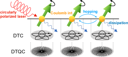
Figure 1: Schematic illustration of time crystals in Hubbard model. The curves on the upper (lower) disks indicate the trajectories of the spin dynamics in the DTC (DTQC) phase.

Floquet dynamical symmetry and time crystals.— We begin by considering periodically-driven dissipative systems for a well-defined formulation and will discuss isolated systems later. For this purpose, we focus on the Floquet-Lindblad master equation Ho et al. (1986); Prosen and Ilievski (2011); Vorberg et al. (2013); Hartmann et al. (2017) ($\hbar=1$ throughout this Letter):

$$\frac{d\rho}{dt}=\mathcal{L}_{t}(\rho)=-i[H(t),\rho]+\gamma\sum_{k}\left(L_{k}\rho L_{k}^{\dagger}-\frac{1}{2}\{L_{k}^{\dagger}L_{k},\rho\}\right),$$ (1)

which describes trace-preserving nonunitary dynamics for the density matrix $\rho$. Here, $H(t)=H(t+T)$ is a time-periodic Hamiltonian describing the unitary part of the evolution, and $L_{k}$’s are the Lindblad operators representing the Markovian dissipation by an environment coupling to the system.

The solution of Eq. (1) is formally given by $\rho(t)=\mathcal{V}(t,0)\rho(0)$, where $\mathcal{V}(t,t^{\prime})\equiv\mathcal{T}\exp(\int_{t^{\prime}}^{t}\mathcal{L}_{s}ds)$ is the time evolution superoperator from $t^{\prime}$ to $t$. Due to the periodicity of $\mathcal{L}_{t}=\mathcal{L}_{t+T}$, we can decompose $\mathcal{V}(t,0)$ into a stroboscopic evolution and a micromotion: $\mathcal{V}(t,0)=\mathcal{V}(\tilde{t},0)\mathcal{U}_{F}^{\ell}$, where $t=\tilde{t}+\ell{T}$   ($0\leq\tilde{t}<T,\ell\in\mathbb{N}$), and $\mathcal{U}_{F}=\mathcal{V}(T,0)$ is the one-cycle time evolution superoperator. The long-time behavior ($\ell\rightarrow\infty$) is characterized by $\mathcal{U}_{F}$. If $\mathcal{U}_{F}$ is diagonalizable $\mathcal{U}_{F}(\rho_{j})=z_{j}\rho_{j}$   ($j=1,\cdots,D^{2}$, $D$ is the Hilbert-space dimension), the formal solution of Eq. (1) is given by $\rho(t)=\mathcal{V}(\tilde{t},0)\sum_{j}a_{j}z_{j}^{\ell}\rho_{j}$, where $a_{j}$ is an expansion coefficients of $\rho(0)=\sum_{j}a_{j}\rho_{j}$. Note that the trace-preserving nature guarantees $|z_{j}|\leq 1$ and there exists at least one eigenvalue $z_{j}=1$, and thus we set $z_{1}=1$ Breuer and Petruccione (2002).

The unique nonequilibrium steady state (NESS) appears if all the other eigenvalues except $z_{1}=1$ satisfy $|z_{j\neq 1}|<1$, meaning that $\rho_{j\neq 1}$ are all decaying modes with relaxation time $1/\ln|z_{j\neq 1}|$ Ikeda and Sato (2020). In fact, any initial state asymptotically relax to a unique NESS, $\rho(t)=\mathcal{V}(\tilde{t},0)\sum_{j}a_{j}z_{j}^{\ell}{\rho_{j}}\xrightarrow{\ell\rightarrow\infty}\mathcal{V}(\tilde{t},0)\rho_{1}$ ($a_{1}=1$ due to the trace preservation). This NESS has time-period $T$ by definition of $t=\tilde{t}+\ell{T}$, which means that the long-time behavior of Eq. (1) typically has the discrete time-translation symmetry $\mathbb{Z}$.

The conventional discrete time crystals Gong et al. (2018); Barberena et al. (2019); Lledó et al. (2019); Riera-Campeny et al. (2019); Zhu et al. (2019) appear if there exist several eigenstates with eigenvalues $e^{i\theta}\,(\theta=2\pi/n,\,n\in\mathbb{N})$. For example, when $z_{1}=1$, $z_{2}=-1$, and $|z_{j\neq 1,2}|<1$, any initial state asymptotically relax to the following NESS: $\rho(t)=\mathcal{V}(\tilde{t},0)\sum_{j}a_{j}z_{j}^{\ell}{\rho_{j}}\xrightarrow{\ell\rightarrow\infty}\mathcal{V}(\tilde{t},0)[\rho_{1}+(-1)^{\ell}{a_{2}}\rho_{2}]$. When $a_{2}\neq 0$, the NESS is a time-crystalline state with period $2T$, which implies $\mathbb{Z}\rightarrow\mathbb{Z}/2$ symmetry breaking. From now on, we call the eigenstate with eigenvalue 1 as a Floquet steady state, and that with eigenvalue $e^{i\theta}\,$($\neq 1$ with $\theta\in\mathbb{R}$) as a Floquet coherent state.

Now we introduce the Floquet dynamical symmetry (FDS), which leads to unconventional time crystals. First, we define the FDS for the unitary one-cycle time evolution operator $U_{F}=\mathcal{T}\exp[-i\int_{0}^{T}{ds}H(s)]$ and the dissipation $L_{k}$ as follows:

$$\begin{aligned} &\hskip 28.45274ptU_{F}AU_{F}^{\dagger}=e^{-i\lambda T}A,\\ &[L_{k},A(t)]=[L_{k}^{\dagger},A(t)]=0,\quad\forall k,t\end{aligned}$$ (2)

where $A(t)=U(t)AU^{\dagger}(t)$ is an FDS operator at time $t$ ($U(t)=\mathcal{T}e^{-i\int_{0}^{t}{ds}H(s)},A(0)=A,A(T)=e^{-i\lambda T}A$), and $\lambda$ is a real number. This definition is a natural extension of the strong dynamical symmetry in time-independent systems Buča et al. (2019); Tindall et al. (2020), which is defined as $[H,A]=\lambda{A}$ and $[L_{k},A]=[L_{k}^{\dagger},A]=0$ (e.g., the Zeeman Hamiltonian $H=\lambda{S^{z}}$ and the raising operator $A=S^{+}$ satisfy this relation, $[H,A]=\lambda A$). We note that the dissipation $L_{k}$ is not required for the FDS, and the time crystals can appear even in isolated systems, as we will show later.

The FDS protects some quantum coherence and prevents the system from relaxing to the unique NESS. We remark that the FDS (2) implies $\mathcal{U}_{F}(A\rho)=e^{-i\lambda{T}}A\mathcal{U}_{F}(\rho)$ and $\mathcal{U}_{F}(\rho{A}^{\dagger})=e^{i\lambda{T}}\mathcal{U}_{F}(\rho)A$ for any $\rho$ (see Supplemental Material S1). Thus, given that $\rho_{s}$ is a Floquet steady state satisfying $\mathcal{U}_{F}(\rho_{s})=\rho_{s}$, $\rho_{mn}=A^{m}\rho_{s}(A^{\dagger})^{n}$ are the Floquet steady ($m=n$) and coherent ($m\neq{n}$) states,

$$\mathcal{U}_{F}(\rho_{mn})=e^{i(n-m)\lambda T}\rho_{mn}.$$ (3)

If there are no other Floquet steady and coherent states except $\rho_{mn}$, we obtain the long-time behavior from them,

$$\rho(t)\xrightarrow{\ell\rightarrow\infty}\sum_{mn}\mathcal{V}(\tilde{t},0)[c_{mn}e^{i(n-m)\lambda\ell T}\rho_{mn}]\equiv\rho_{\infty}(t),$$ (4)

where $c_{mn}$ is expansion coefficients of $\rho_{mn}$. There exist two typical energy (or time) scales in $\rho_{\infty}(t)$. One is the Floquet frequency $\omega=2\pi/T$ stemming from the periodicity of $\mathcal{V}(\tilde{t},0)$, and the other is $\lambda$ characterized by the FDS.

Depending on whether the ratio $\lambda/\omega$ is a rational number or not, the long-time behavior (4) represents the DTC or DTQC, respectively. If $\lambda/\omega\in\mathbb{Q}$, i.e., $\lambda/\omega=q/p$ for some coprime integers $p$ $(\geq 2)$ and $q$, the DTC emerges: $\rho_{\infty}(t+T)\neq\rho_{\infty}(t)$, but $\rho_{\infty}(t+pT)=\rho_{\infty}(t)$ holds true. This means the discrete time-translation symmetry breaking, $\mathbb{Z}\rightarrow\mathbb{Z}/p$. On the other hand, if $\lambda/\omega\notin\mathbb{Q}$, the discrete time-translation symmetry $\mathbb{Z}$ is broken, but there is no integer $p$ such that $\rho_{\infty}(t+pT)=\rho_{\infty}(t)$. Nevertheless, there exist an infinite number of times $s$ such that $\rho_{\infty}(t+s)$ is arbitrarily close to $\rho_{\infty}(t)$. Thus, the dynamics is quasiperiodic, and we call it the DTQC. Note that these time crystals are protected by the FDS and robust against the perturbations respecting the symmetry.

Tunable time crystals in dissipative Hubbard models.— Here we present simple models exhibiting the time crystals protected by the FDS: spin-$S$ Bose- or Fermi-Hubbard models under a circularly polarized ac field in $d$ dimensions. The Hamiltonian $H(t)=H_{0}+V(t)$ is

$$\begin{aligned} &H_{0}=-J\sum_{\braket{i,j},\sigma}(c^{\dagger}_{i,\sigma}c_{j,\sigma}+\text{h.c.})+\frac{U}{2}\sum_{j}n_{j}^{2}+\frac{K}{2}\sum_{\braket{i,j}}n_{i}n_{j},\\ &V(t)=B\left(S^{x}\cos\omega t+S^{y}\sin\omega t\right),\end{aligned}$$ (5)

where $c_{j,\sigma}(c_{j,\sigma}^{{\dagger}})$ is the annihilation (creation) operator for the boson or fermion with spin $\sigma\in\{-S,\cdots,S\}$ on the site $j$, and $n_{j}=\sum_{\sigma}c_{j,\sigma}^{{\dagger}}c_{j,\sigma}$ is the particle number operator. The operators for the spin at site $j$ and for the total spin are denoted by $S_{j}^{\mu}$ and $S^{\mu}=\sum_{j}S_{j}^{\mu}\,(\mu=x,y,z)$. The nearest-neighbor interaction is added to break the integrability of the model in $d=1$.

We consider the dissipation described by local dephasing Lindblad operators acting on each site, $L_{j}=n_{j}$, which suppresses the particle number fluctuation. We will discuss later how to realize them experimentally.

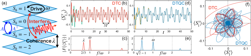
Figure 2: (a) Mechanism of time crystals by Floquet dynamical symmetry. Each sheet represents the different spin sectors. The periodic drive and the quantum coherence interfere with each other. (b) DTC time evolutions of $\braket{S^{y}_{j}(t)}$ (red: $j=1$, green: $j=3$) and (c) the Fourier component ($j=1$). (d) DTQC time evolutions of $\braket{S^{y}_{j}(t)}$ (blue: $j=1$, yellow: $j=3$) and (e) the Fourier component ($j=1$). We have performed the Fourier transformation for $t\in[20,100]$ by convoluting the window function $w(t)=\exp[-(t-60)^{2}/20^{2}]$. (f) Trajectories of time evolution in $(S_{1}^{x},S_{1}^{y})$-plane. The red (blue) curve denotes the DTC (DTQC) trajectory. The parameters are $L=6,J=U=K=1,\gamma=0.1,\omega=\pi$, and $B=4\pi/3$ ($B=\pi$) for the DTC (DTQC).

Our model has the FDS in the one cycle of the ac field. To show this, we consider a unitary transformation to the rotating frame Slichter (1996); Kohler et al. (2005); Takayoshi et al. (2014); Zhao et al. (2019), $\rho_{\text{RF}}(t)=R(t)\rho(t)R(t)^{\dagger}$ ($R(t)=e^{i\omega{t}S^{z}}$). Then, the Hamiltonian is transformed to the Hubbard model in an effective static magnetic field, $H_{\text{RF}}=R(t)[H(t)-i\partial_{t}]R(t)^{\dagger}=H_{0}+\bm{h}\cdot\bm{S}$, where $\bm{h}=(B,0,\omega)$, while the Lindblad operators are invariant. Therefore, in the rotating frame, the system has the strong dynamical symmetry Buča et al. (2019); Tindall et al. (2020), or the FDS $U_{F}^{\text{RF}}A(U_{F}^{\text{RF}})^{\dagger}=e^{-i\lambda T}A$ and $[L_{j},A]=[L_{j}^{\dagger},A]=0$, where $U_{F}^{\text{RF}}$ is the unitary one-cycle time evolution operator in the rotating frame, $A=S_{\bm{h}}^{+}$ is the total spin raising operator along the effective magnetic field $\bm{h}$, and

$$\lambda=|\bm{h}|=\sqrt{\omega^{2}+B^{2}}\quad(\text{mod}\;\omega).$$ (6)

Going back to the original frame, we have $U_{F}=R^{\dagger}(T)U_{F}^{\text{RF}}R(0)=U_{F}^{\text{RF}}$ up to the phase factor and $A(t)=R^{\dagger}(t)AR(t)=S^{+}_{\bm{h}(t)}$, where $S^{+}_{\bm{h}(t)}$ is the raising operator along $\bm{h}(t)=(B\cos\omega t,B\sin\omega t,\omega)$, obtaining the FDS

$$\begin{aligned} &\hskip 28.45274ptU_{F}S_{\bm{h}}^{+}U_{F}^{\dagger}=e^{-i\lambda T}S_{\bm{h}}^{+},\\ &[L_{j},S^{+}_{\bm{h}(t)}]=[L_{j}^{\dagger},S^{+}_{\bm{h}(t)}]=0,\quad\forall j,t.\end{aligned}$$ (7)

We remark that the FDS also exists under elliptically-polarized fields for spin-$1/2$ Fermi-Hubbard model, for which we cannot find a rotating frame giving a static Hamiltonian (see Supplemental Material S2). Thus, the FDS is a more general concept not restricted to the rotating-frame argument.

The FDS (7) gives the Floquet steady and coherent states $\rho_{mn}=(S_{\bm{h}}^{+})^{m}\rho_{s}(S_{\bm{h}}^{-})^{n}$ with eigenvalue $e^{i(n-m)\lambda T}$ in Eq. (3). This implies that the FDS protects the quantum coherence between the different spin sectors labelled by $S_{\bm{h}}=\bm{h}\cdot\bm{S}/|\bm{h}|$, which are Zeeman-split by $\lambda$ in the Floquet spectrum (see Fig. 2 (a)). Meanwhile, the quantum coherence within each sector are eliminated by dissipation (and quantum thermalization discussed below), and the Floquet steady state oscillating with frequency $\omega$ appears within each sector. These Floquet steady states are superposed and the two scales, $\lambda$ and $\omega$, interfere with each other, giving rise to the DTC and DTQC.

We emphasize the tunability of our time crystals. As shown before, the periodicity of these time crystals depend on the ratio $\lambda/\omega=\sqrt{1+(B/\omega)^{2}}$, which can be tuned only by varying the field strength $B$ with $\omega$ fixed. If $\lambda/\omega=q/p$ ($\leftrightarrow$ $B=\omega\sqrt{(q/p)^{2}-1}$) with coprime integers $p$ and $q$, the DTC appears with period $pT$, whereas, if $\lambda/\omega\notin\mathbb{Q}$, the DTQC appears.

Synchronized DTC and DTQC in the Hubbard model.— Let us numerically demonstrate the DTC and DTQC by taking the spin-1/2 Fermi-Hubbard model in one dimension with $L$ sites. We assume the periodic boundary condition and solve Eq. (1) by the fourth-order Runge–Kutta method. Throughout this Letter, the initial state is a $1/4$-filled state where the $j$-th site ($j=1,2,\cdots,L/2$) is occupied by one fermion, and every third fermions are polarized along $-x$ and all others are polarized along $x$ (we assume $L$ is a multiple of 6).

Figure 2 (b) shows the time evolution of $\braket{S_{j}^{y}(t)}(j=1,3)$ in the DTC phase for $\omega=\pi$ and $\lambda=2\pi/3$. After the initial relaxation dynamics, $\braket{S_{j}^{y}(t)}$ oscillates with period $3T=6$, which is the least common multiple of $T=2\pi/\omega=2$ and $2\pi/\lambda=3$. This means the discrete time-translation symmetry breaking $\mathbb{Z}\rightarrow\mathbb{Z}/3$. The rationality of two peaks in the Fourier space (Fig. 2 (c)) at $f=\omega$ and $\lambda$ also shows the commensurability. Moreover, the dynamics of $\braket{S_{1}^{y}(t)}$ and $\braket{S_{3}^{y}(t)}$ are synchronized after relaxation, which implies all the Floquet steady and coherent states are translationally symmetric Buča et al. (2019); Tindall et al. (2020).

On the other hand, Fig. 2 (d) shows the time evolution in the DTQC phase for $\omega=\pi$ and $\lambda=(\sqrt{2}-1)\pi$, where the synchronized spins oscillate aperiodically. The irrationality of two peaks, $f=\omega$ and $\lambda$, in the Fourier space (Fig. 2 (e)) shows the incommensurability of the time crystal and no perfect periodicity.

The trajectories of the DTC and DTQC dynamics in the $(S^{x}_{1},S^{y}_{1})$-plane are shown in Fig. 2 (f). The trajectory of the DTC dynamics (red) behaves as the limit cycle, and gradually converges to the star-shaped closed curve. On the other hand, the trajectory of the DTQC dynamics (blue) never converges to a closed curve, and keep rotating aperiodically on the plane. This aperiodic dynamics highlights the difference from the DTC.

Quantum-thermalization-induced time crystals without dissipation.— Until now, we have considered the dissipative systems to clarify the role of the FDS and the mechanism of the time crystals. However, the time crystals do not necessarily require the dissipation. According to the recent studies D’Alessio et al. (2016); Eisert et al. (2015); Mori et al. (2018), an isolated quantum system without dissipation exhibits thermalization (or, more precisely, equilibration) due to dephasing between many-body energy eigenstates when the system size is large enough Tasaki (1998); Reimann (2008); Short (2011). The quantum thermalization (equilibration) effectively plays the role of dissipation and eliminates quantum coherence except those protected by the FDS, bringing about the time crystals .

We demonstrate the time crystal protected by the FDS without dissipation (i.e., $\gamma=0$) in Fig. 3. Both in the time profile and Fourier spectrum, we observe a clear time-crystalline behavior at $L=12$ (upper panels) whereas a noisy one at $L=6$ (lower panels). This noise derives from the imperfect dephasing as a finite-size effect and typically decreases exponentially in the system size.

The time crystals in isolated systems are interpreted by the maximum entropy principle under multiple conserved quantities Jaynes (1957) that is also known as the generalized Gibbs ensemble (GGE) Rigol et al. (2007); Medenjak et al. (2019) . The key to this interpretation is the unconventional stroboscopically-conserved quantities that are derived from the FDS. To show this intuitively, we focus on the DTC case with $\lambda/\omega=q/p$ $(p\geq 2)$. One can easily show that the FDS $U_{F}AU_{F}^{\dagger}=e^{-i\lambda T}A$ leads to such quantities after $p$ steps:

$$[U_{F}^{p},A]=[U_{F}^{p},A^{\dagger}]=0.$$ (8)

These stroboscopically-conserved quantities, $A$ and $A^{\dagger}$, constrain the dynamics and lead, after a long time, to the GGE at $t=npT$ ($n\in\mathbb{N}$): $\rho_{\text{TC}}(t=npT)=\exp\left[-\sum_{i}\beta_{i}Q_{i}-\mu A-\mu^{\ast}A^{\dagger}\right]/Z$. Here $Z$ is the partition function, $\mu$ is the chemical potential for $A$, and $Q_{i}$ and $\beta_{i}$ are the conventional local conserved quantities of $U_{F}$ and their generalized inverse temperatures. Acting the time evolution operator $U(t_{0})$ from $t=npT$ to $t=t_{0}+npT$ ($t_{0}\in[0,pT)$), we obtain the time-dependent GGE $\rho_{\text{TC}}(t_{0}+npT)=U(t_{0})\rho_{\text{TC}}(npT)U^{\dagger}(t_{0})$:

$$\rho_{\text{TC}}(t)=\frac{\exp\left[-\sum_{i}\beta_{i}Q_{i}(t)-\mu(t)\tilde{A}(t)-\mu(t)^{\ast}\tilde{A}^{\dagger}(t)\right]}{Z},$$ (9)

where $Q_{i}(t)=U(t)Q_{i}U^{\dagger}(t)$, $\tilde{A}(t)=e^{i\lambda t}U(t)AU^{\dagger}(t)$, and $\mu(t)=\mu e^{-i\lambda t}$. Remarkably, under a certain assumption, this result (9) also holds in the DTQC case where there exist no stroboscopically-conserved quantities (see Supplemental Material S4).

The time-dependent GGE (9) is a two-color generalization of the previous ones Lazarides et al. (2014); Medenjak et al. (2019). Whereas $Q_{i}(t)$ and $\tilde{A}(t)$ have the period $T=2\pi/\omega$ of the external field, $\mu(t)$ has a different one $T_{\lambda}=2\pi/\lambda$ of the FDS. These two periods, depending on their ratio, give the DTC and DTQC in isolated systems. The synchronization implies the translation symmetry of $Q_{i}(t)$ and $\tilde{A}(t)$.

In deriving Eq. (9), we have implicitly assumed that there are no other FDS than $A$. This assumption is known to break down in free and many-body-localized systems that have an extensive number of local dynamical symmetries. In these systems, the dense and incommensurate frequencies associated with the multiple FDSs can destroy time crystals Essler and Fagotti (2016); Khemani et al. (2019); Booker et al. (2020). It is an open question to elucidate the roles of these multiple FDSs.

Finally, we remark the robustness of our time crystals against disorder. As shown above, the time-crystalline nature relies only on the FDS, and the disorder never disturbs the time crystals as long as it respects the FDS (and there exist no other FDS). For example, random onsite potentials Prelovšek et al. (2016), which are SU($2$)-symmetric unlike random onsite magnetic fields, do not destroy the time crystals both in the dissipative and isolated systems (see Supplemental material S5).

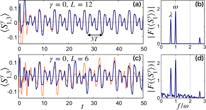
Figure 3: Time profile $\braket{S^{y}_{j}(t)}$ (left) and its Fourier spectrum (right) calculated in the absence of dissipation ($\gamma=0$). The upper (lower) panels correspond to $L=12$ ($L=6$), and the navy (orange) curve to site $j=1$ ($j=3$). The other parameters are $J=U=K=1,\omega=\pi$, and $B=4\pi/3$ (DTC phase).

Discussions and conclusions.— In this Letter, we have introduced the FDS and proposed a new class of time crystals protected by the FDS. Although we have focused on the circularly polarized ac field, the time crystals also appear in the Hubbard model with static and linearly-polarized ac fields both along the $z$-direction. This is because a trivial dynamical symmetry holds at any time, $[H(t),S^{+}]\propto S^{+}$. This setup is known as the electron spin resonance (ESR) in the condensed matter physics Weil (1984).

Our model (5) can be realized in ultracold atoms on an optical lattice Jaksch and Zoller (2005); Esslinger (2010). The hyperfine states of the atom behave as a pseudospin, and the coupling between the states, or the Zeeman effect on the pseudospin, is manipulated by radio waves Esslinger (2010). State-of-the-art laser technology enables us to control the strength and frequency of the coupling, realizing the highly tunable time crystals. Also, the particle number dephasing $L_{j}=n_{j}$ is achieved by immersing the optical lattice into a Bose-Einstein condensate Klein et al. (2007); Mayer et al. (2019).

Finally, we note that our model (5) actually has the SU($N$) symmetry with $N=2S+1$ Honerkamp and Hofstetter (2004); Cazalilla et al. (2009); Gorshkov et al. (2010). Such an SU($N$)-symmetric Hubbard model has been realized in ultracold atoms Taie et al. (2010); Zhang et al. (2014); Scazza et al. (2014), and has attracted much attention recently. This model could accommodate more exotic time crystals with multiple input frequencies and the extended FDS due to the enlarged algebraic structure. Generalizing our arguments to the SU($N$) systems is an interesting open question, where time crystals should meet large Lie algebras together with cold atom experiments.

Acknowledgements.— We thank K. Fukai and H. Tsunetsugu for fruitful discussions. This work was supported by JSPS KAKENHI Grant No. JP18K13495. K. C. acknowledges the financial support provided by the Advanced Leading Graduate Course for Photon Science at the University of Tokyo.

Note added.— In preparing this manuscript, we have become aware of an independent work Medenjak et al. (2020), where the FDS and its consequences are briefly discussed.

Supplemental Materials

I S1. Derivation of Floquet steady and coherent states

Here we briefly prove that the Floquet dynamical symmetry (FDS) leads to

$$\begin{aligned} &\mathcal{U}_{F}(A\rho)=e^{-i\lambda T}A\mathcal{U}_{F}(\rho),\\ &\mathcal{U}_{F}(\rho A^{\dagger})=e^{i\lambda T}\mathcal{U}_{F}(\rho)A,\end{aligned}$$ (1)

for any $\rho$, and thus the time crystals (see Eqs. (3) and (4) in the main text). To this end, let us introduce superoperators $\hat{O}_{L}$ and $\hat{O}_{R}$ ($O$ is a usual operator), which act on the density matrix from the left and right sides such that $\hat{O}_{L}\rho=O\rho$ and $\hat{O}_{R}\rho=\rho O^{\dagger}$.

Using FDS superoperators $\hat{A}_{L}$ and $\hat{A}_{R}$, Eq. (1) reads

$$\begin{aligned} &\hat{\mathcal{U}}_{F}\hat{A}_{L}=e^{-i\lambda T}\hat{A}_{L}\hat{\mathcal{U}}_{F},\\ &\hat{\mathcal{U}}_{F}\hat{A}_{R}=e^{i\lambda T}\hat{A}_{R}\hat{\mathcal{U}}_{F},\end{aligned}$$ (2)

where $\hat{\mathcal{U}}_{F}=\mathcal{T}\exp[\int_{0}^{T}\hat{\mathcal{L}}_{s}ds]$ is the one-cycle time evolution superoperator, and the Liouvillian $\hat{\mathcal{L}}_{t}$ is a sum of the unitary part $\hat{\mathcal{H}}_{t}$ and the dissipative one $\hat{\mathcal{D}}$, $\hat{\mathcal{L}}_{t}=\hat{\mathcal{H}}_{t}+\hat{\mathcal{D}}$. Note that the FDS $[L_{k},A(t)]=[L_{k}^{\dagger},A(t)]=0$ leads to commutation relations $[\hat{\mathcal{D}},\hat{A}_{L}(t)]=[\hat{\mathcal{D}},\hat{A}_{R}(t)]=0$.

To prove the upper one in Eq. (2) (the lower one is also proven by a similar argument), we consider a superoperator $\hat{X}(t)=\hat{\mathcal{U}}(t)\hat{A}_{L}\hat{\mathcal{U}}(t)^{-1}$, where $\hat{\mathcal{U}}(t)=\mathcal{T}\exp[\int_{0}^{t}\hat{\mathcal{L}}_{s}ds]$ is the time evolution superoperator from 0 to $t$, and $\hat{\mathcal{U}}(t)^{-1}=\tilde{\mathcal{T}}\exp[-\int_{0}^{t}\hat{\mathcal{L}}_{s}ds]$ is its inverse ($\tilde{\mathcal{T}}$ denotes the anti-time-ordering operator). By using the relations $\partial_{t}\hat{\mathcal{U}}(t)=\hat{\mathcal{L}}_{t}\hat{\mathcal{U}}(t)$ and $\partial_{t}\hat{\mathcal{U}}(t)^{-1}=-\hat{\mathcal{U}}(t)^{-1}\hat{\mathcal{L}}_{t}$, we have a time evolution equation of $\hat{X}(t)$:

$$\partial_{t}\hat{X}(t)=[\hat{\mathcal{L}}_{t},\hat{X}(t)].$$ (3)

One can easily show that the solution of this equation is $\hat{X}(t)=\hat{A}_{L}(t)$ because of $\partial_{t}\hat{A}_{L}(t)=[\hat{\mathcal{H}}_{t},\hat{A}_{L}(t)]$ and $[\hat{\mathcal{D}},\hat{A}_{L}(t)]=0$ that is derived by the FDS. Therefore, we obtain Eq. (2) by $\hat{\mathcal{U}}_{F}\hat{A}_{L}\hat{\mathcal{U}}_{F}^{-1}=\hat{X}(T)=\hat{A}_{L}(T)=e^{-i\lambda T}\hat{A}_{L}$, and thus Eq. (1), where we have used the FDS, $A(T)=U_{F}AU_{F}^{\dagger}=e^{-i\lambda T}A$.

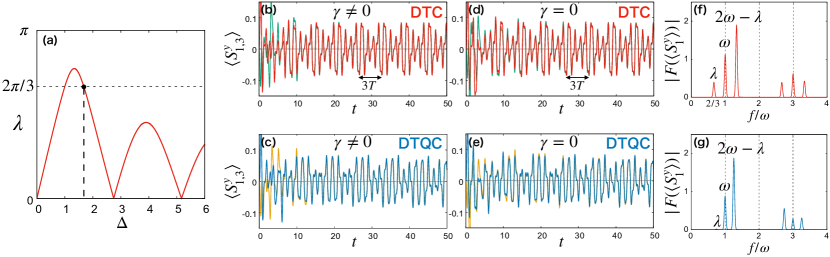
Figure S1: (a) Strength of effective magnetic field for $\omega=\pi$ and $B=4\pi/3$ with varied $\Delta$. (b,d) DTC time evolutions of $\braket{S^{y}_{j}(t)}$ (red: $j=1$, green: $j=3$) at $\Delta\simeq 1.673$ ($\lambda=2\pi/3$) in (b) the dissipative and (d) isolated systems. (c,e) DTQC time evolutions of $\braket{S^{y}_{j}(t)}$ (blue: $j=1$, yellow: $j=3$) at $\Delta=1.5$ in (c) the dissipative and (e) isolated systems. The parameters are $J=U=K=1,\omega=\pi,B=4\pi/3$, and $\gamma=0.1$ for (b,c) ($\gamma=0$ for (d,e)). The system sizes are $L=6$ for (b,c) and $L=12$ for (d,e). (f,g) Fourier components of $\braket{S^{y}_{1}(t)}$ in (b) and (c) respectively. We have performed the Fourier transformation for $t\in[20,100]$ by convoluting the window function $w(t)=\exp[-(t-60)^{2}/20^{2}]$.

II S2. Hubbard model under elliptically polarized ac field

Here, we show that the spin-1/2 Fermi-Hubbard model under an elliptically polarized ac field also possesses the FDS and exhibits the time-crystalline behaviors. The Hamiltonian $H_{\text{el}}(t)=H_{0}+V_{\text{el}}(t)$ is given by

$$\begin{aligned} H_{0}&=-J\sum_{\braket{i,j}\sigma}(c^{\dagger}_{i\sigma}c_{j\sigma}+\text{h.c.})\\ &\hskip 14.22636pt+(U/2)\sum_{j}n_{j}^{2}+(K/2)\sum_{\braket{i,j}}n_{i}n_{j},\end{aligned}$$ (4)

$$V_{\text{el}}(t)=\sum_{j}V_{j}(t)=B\left(\Delta S^{x}\cos\omega t+S^{y}\sin\omega t\right),$$ (5)

where $V_{j}=B\left(\Delta S^{x}_{j}\cos\omega t+S^{y}_{j}\sin\omega t\right)$ denotes the Zeeman coupling to the elliptically polarized field at the $j$-th site. The parameter $\Delta$ characterizes the ellipticity, and $\Delta=1$ corresponds to the circular polarization.

To show the FDS, we consider the one-cycle time evolution operator under $H_{\text{el}}(t)$, $U_{F}^{\text{el}}=\mathcal{T}\exp[-i\int_{0}^{T}dtH_{\text{el}}(t)]$. By using the commutation relations $[H_{0},V_{\text{el}}(t)]=0$ and $[V_{i}(t),V_{j}(t^{\prime})]=0\,\,(i\neq j)$, we have $U_{F}^{\text{el}}=e^{-iH_{0}T}\bigotimes_{j}U_{j}$, where $U_{j}=\mathcal{T}\exp[-i\int_{0}^{T}dtV_{j}(t)]$ is a unitary operator acting on the $j$-th site, where the Hilbert space is 4-dimensional. We remark that $V_{j}(t)$ acts nontrivially only on the two-dimensional one-body subspace (one should also note $\text{tr}[V_{j}(t)]=0$). In this subspace, since $U_{j}$ is a $2\times 2$ matrix, its logarithm can be expanded by the Pauli matrices, or the spin operators: $U_{j}=e^{-i\bm{h}_{\text{eff}}\cdot\bm{S}_{j}T}$, where $\bm{h}_{\text{eff}}$ is the expansion coefficients of the spin operators (we have ignored the constant term). Note that this expression is valid on the total 4-dimensional Hilbert space. Summing up all the terms, we obtain the Floquet Hamiltonian

$$H_{F}^{\text{el}}=\frac{i}{T}\log U_{F}^{\text{el}}=H_{0}+\bm{h}_{\text{eff}}\cdot\bm{S}.$$ (6)

This result means that the stroboscopic time evolution under $H_{\text{el}}(t)$ is identical to that under $H_{F}$, namely the Hubbard model in the static magnetic field $\bm{h}_{\text{eff}}$. The dynamical symmetry of the Floquet Hamiltonian (6), $[H_{F},S^{+}_{\bm{h}_{\text{eff}}}]=|\bm{h}_{\text{eff}}|S^{+}_{\bm{h}_{\text{eff}}}$, gives rise to the FDS:

$$U_{F}^{\text{el}}S^{+}_{\bm{h}_{\text{eff}}}(U_{F}^{\text{el}})^{\dagger}=e^{-i\lambda T}S^{+}_{\bm{h}_{\text{eff}}},$$ (7)

where $S^{+}_{\bm{h}_{\text{eff}}}$ is a total spin raising operator along the effective magnetic field $\bm{h}_{\text{eff}}$, and $\lambda=|\bm{h}_{\text{eff}}|$. This FDS leads to the time crystals in the Hubbard model driven by the elliptically polarized ac field. We note that, unlike the case of the circularly polarized ac field, this time crystals cannot be understood by the unitary transformation to the rotating frame since the time-dependence remains even in the rotating frame.

Let us numerically demonstrate our results. Figure S1 (a) shows the $\Delta$-dependence of $\lambda$ for $\omega=\pi$ and $B=4\pi/3$. By tuning $\Delta$ as $\lambda=2\pi/3$ based on Fig. S1 (a), we obtain the DTC dynamics with period $3T=6$, which is the least common multiple of $T=2\pi/\omega=2$ and $2\pi/\lambda=3$, both in the dissipative and isolated systems (Figs. S1 (b) and (d)). Moreover, the spin dynamics at the different sites are synchronized after the first relaxation due to dissipation and quantum thermalization. On the other hand, for a not-fine-tuned $\Delta$, the synchronized DTQC dynamics appear both in the dissipative and isolated systems (Figs. S1 (c) and (e)). These results are also confirmed by the Fourier analysis (Figs. S1 (f) and (g)), where we see peaks at $\omega$ and $\lambda$ together with their harmonics and sum (difference) frequencies, which implies the appearance of the time-crystalline nature.

S3. Time crystals in isolated integrable systems

The key mechanisms of the time crystals in the isolated systems are the FDS and the equilibration to the stationary state with small time-fluctuation in the stroboscopic sense, although we have roughly used the term “thermalization” in the main text. Therefore, we expect that not only the nonintegrable systems exhibiting the thermalization but also the integrable systems not exhibiting the thermalization show the time-crystalline behavior in the thermodynamic limit due to the equilibration.

Figure S2 shows the spin dynamics in (a) the extended Hubbard, (b) the usual Hubbard, and (c,d) the free fermion models driven by the circularly polarized ac field, respectively, for (a,b,c) $L=12$ and (d) $L=900$. As shown in the figure, the Hubbard model with $L=12$ (Fig. S2 (b)) exhibits the time crystals as well as the extended Hubbard model (Fig. S2 (a)) in spite of the integrability. On the other hand, the dynamics of the free fermion system with $L=12$ (Fig. S2 (c)) seems quite noisy. This implies that the free fermion model does not equilibrate yet due to its high symmetry even for $L=12$. As the system size increases, the equilibration becomes more accurate, and the time-crystalline behavior finally appears for $L=900$ (Fig. S2 (d)).

We note that the free fermion systems have an extensive number of (local) dynamical symmetries. For example, the spinless fermions with the quadratic Hamiltonian $H=\sum_{k}\epsilon_{k}c_{k}^{\dagger}c_{k}$ have the dynamical symmetries $[H,c_{k}^{\dagger}]=\epsilon_{k}c_{k}^{\dagger}$, $[H,c_{k}^{\dagger}c_{l}]=(\epsilon_{k}-\epsilon_{l})c_{k}^{\dagger}c_{l}$, and so on, where $c_{k}$ ($c_{k}^{\dagger}$) is an annihilation (creation) operator. These dense and incommensurate frequencies $\epsilon_{k}$ can destroy the time crystals in general Essler and Fagotti (2016); Booker et al. (2020). Nevertheless, as shown in Fig. S2 (d), the multiple dynamical symmetries do not destroy the time-crystalline nature for the spins in our model. However, they can be important in other situations such as the case with the particle number fluctuation, where there can exist quantum coherence between $\ket{\psi}$ and $c_{k}^{\dagger}\ket{\psi}$ protected by the dynamical symmetry $[H,c_{k}^{\dagger}]=\epsilon_{k}c_{k}^{\dagger}$. The complete elucidation of the role of the multiple dynamical symmetries in free systems is an open question.

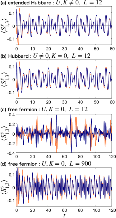
Figure S2: Time evolution of $\braket{S^{y}_{j}(t)}$ (navy: $j=1$, orange: $j=3$) in (a) extended Hubbard model, (b) usual Hubbard model, and (c,d) free fermion model without dissipation. The parameters are $J=1,\gamma=0,\omega=\pi,B=4\pi/3$, and $(U,K)=$ (a) $(3,1)$, (b) $(3,0)$, and (c,d) $(0,0)$. The system sizes are $L=12$ for (a,b,c) and $L=900$ for (d).

S4. GGE description of time crystals protected by Floquet dynamical symmetry

Here we show the time-dependent GGE of the time crystals protected by the FDS in the isolated systems.

A. Preliminary: case of time-independent Hamiltonian

For preliminary, let us consider the static Hamiltonian $H$ with the usual extended dynamical symmetry $[H,A]=\lambda A$ (this setup and its conclusion were discussed in Ref. Medenjak et al. (2019)). The extended dynamical symmetry leads to the stroboscopically-conserved quantity:$A_{H}(s+nT_{\lambda})=A_{H}(s)$ in the Heisenberg picture for each $s\in[0,T_{\lambda})$ with $T_{\lambda}=2\pi/\lambda$ and $n\in\mathbb{N}$. This unconventional conserved quantity prevents the system from relaxing to the stationary state and gives rise to the time-dependent GGE with period $T_{\lambda}$:

$$\rho(t)=\frac{\exp[-\sum_{i}\beta_{i}(t)Q_{i}-\mu(t)A-\mu^{\ast}(t)A^{\dagger}]}{Z_{t}}.$$ (8)

Here $Z_{t}$ is the periodic partition function, $\mu(t)$ is the periodic chemical potential for $A$, and $Q_{i}$ and $\beta_{i}(t)$ are the conventional local conserved quantities of $H$ and their periodic generalized inverse temperatures (the time-dependence of $\beta_{i}(t)$ could stems from the noncommutativity between $Q_{i}$’s and $A$, but in fact, $\beta_{i}(t)$ does not depend on time as shown below). The chemical potential $\mu(t)$ and the generalized inverse temperatures $\beta_{i}(t)$ are determined by the following relations for any $t$:

$$\begin{aligned} \braket{\psi(t)}{Q_{i}}{\psi(t)}&=\text{tr}[Q_{i}\rho(t)],\\ \braket{\psi(t)}{A}{\psi(t)}&=\text{tr}[A\rho(t)].\end{aligned}$$ (9)

These relations are satisfied by $\beta_{i}(t)=\beta_{i}$ and $\mu(t)=\mu e^{-i\lambda t}$, where $\beta_{i}$ and $\mu$ are time-independent quantities satisfying Eqs. (9) at $t=0$. To prove this, we have used $U^{\dagger}(t)AU(t)=e^{i\lambda t}A$, $U^{\dagger}(t)Q_{i}U(t)=Q_{i}$, and $\rho(t)=U(t)\rho(0)U^{\dagger}(t)$ if $\beta_{i}(t)=\beta_{i}$ and $\mu(t)=\mu e^{-i\lambda t}$. Then, $Z_{t}$ is also time-independent because of $\rho(t)=U(t)\rho(0)U^{\dagger}(t)$. As a result, we obtain

$$\rho(t)=\frac{\exp[-\sum_{i}\beta_{i}Q_{i}-\mu(t)A-\mu^{\ast}(t)A^{\dagger}]}{Z},$$ (10)

where $\mu(t)=\mu(0)e^{-i\lambda t}$.

B. Time-dependent GGE for time crystals protected by FDS

Now we consider the time-periodic Hamiltonian $H(t)=H(t+T)$ with the FDS. To obtain the GGE, we invoke a theoretical trick of introducing a virtual time evolution under the Floquet Hamiltonian $H_{F}=(i/T)\log U_{F}$. Namely, the evolution from time $0$ to $t$ is given by $e^{-iH_{F}t}$ in this virtual evolution. While the real evolution generated by $H(t)$ is different from the virtual one at most times, they coincide with each other at the stroboscopic times $t=nT$ ($n\in\mathbb{N}$). From now on, we call the density matrix obtained by the evolution under $H(t)$ as $\rho_{\text{TC}}(t)$ and that under $H_{F}$ as $\rho_{F}(t)$. Given that they share the initial condition $\rho_{\text{TC}}(0)=\rho_{F}(0)$, we have

$$\rho_{\text{TC}}(nT)=\rho_{F}(nT).$$ (11)

Here we assume that the Floquet Hamiltonian $H_{F}$ has the same local conserved quantities as $U_{F}$ and the extended dynamical symmetry,

$$[H_{F},Q_{i}]=0,\,\,\,[H_{F},A]=\lambda A,$$ (12)

where $Q_{i}$ are local (or few-body) conserved quantities of $U_{F}$: $[U_{F},Q_{i}]=0$. Note that the assumption (12) implies the FDS and holds in the Hubbard models under the circularly and elliptically polarized ac fields discussed in the main text and Sec. S2. Since Eq. (12) means the extended dynamical symmetry, the argument in the previous subsection applies to the present virtual evolution, and we have $\rho_{F}(t)=\exp[-\sum_{i}\beta_{i}Q_{i}-\mu(t)A-\mu^{\ast}(t)A^{\dagger}]/Z$ (see Eq. (10)). Here $Z$ is the partition function, $\mu(t)=\mu e^{-i\lambda t}$ is the periodic chemical potential for $A$, $Q_{i}$ are the local conserved quantities of $H_{F}$ (and, hence, $U_{F}$), and $\beta_{i}$ are the generalized inverse temperatures for them.

The GGE thus obtained for the virtual evolution gives that for the real evolution of interest at the stroboscopic times through Eq. (11). To obtain the GGE at different times, we act the time evolution operator $U(t_{0})$ from $nT$ to $t_{0}+nT$, obtaining the time-dependent GGE $\rho_{\text{TC}}(t_{0}+nT)=U(t_{0})\rho_{\text{TC}}(nT)U^{\dagger}(t_{0})$:

$$\rho_{\text{TC}}(t)=\frac{\exp\left[-\sum_{i}\beta_{i}Q_{i}(t)-\mu(t)\tilde{A}(t)-\mu(t)^{\ast}\tilde{A}^{\dagger}(t)\right]}{Z}.$$ (13)

Here, $Q_{i}(t)=Q_{i}(t_{0})=U(t)Q_{i}U^{\dagger}(t)$ is periodic conserved quantities of $H(t)$, $\tilde{A}(t)\equiv e^{i\lambda t}U(t)AU^{\dagger}(t)$ is a periodic FDS operator, and $\mu(t)=\mu e^{-i\lambda t}$ is the periodic chemical potential for $A$. This result (13) is consistent with Eq. (9) in the main text, which is derived by considering the stroboscopically-conserved quantities of the DTC.

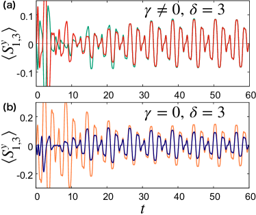
Figure S3: (a) Time evolution of $\braket{S^{y}_{j}(t)}$ (red: $j=1$, green: $j=3$) in dissipative Hubbard model with disordered potential. The parameters are $L=6,J=U=K=1,\gamma=0.1,\delta=3,\omega=\pi$, and $B=4\pi/3$. (b) Time evolution of $\braket{S^{y}_{j}(t)}$ (orange: $j=1$, navy: $j=3$) in isolated Hubbard model with disordered potential. The parameters are $L=12,J=U=K=1,\gamma=0,\delta=3,\omega=\pi$, and $B=4\pi/3$. Both in (a) and (b), we have used one realization for the disorder potentials $\{\epsilon_{j}\}$ rather than the ensemble average, and the realizations for (a) and (b) are different.

In deriving Eq. (13) for the DTC and DTQC, we have assumed the conditions (12). On the other hand, the derivation of Eq. (9) in the main text does not need any assumptions although it is limited to the DTC case. It is an open problem whether the assumption (12) really needs or not in the DTQC case.

S5. Robustness against disorder

Here, we show that the time crystals protected by the FDS are robust against perturbations as long as the FDS is preserved, although the synchronization in the isolated systems may become imperfect. To illustrate this, we consider the disordered onsite potential

$$V_{d}=\sum_{j}\epsilon_{j}n_{j},$$ (14)

where $\epsilon_{j}$’s are independent random variables following the uniform distribution over $(-\delta,\delta)$. This disorder respects the FDS due to the spin-SU(2) symmetry, but breaks the spatial translation symmetry.

In the presence of the dissipation $L_{j}=n_{j}$, not only the time-crystalline nature but also the synchronization are robust against the disorder. Figure S3 (a) shows the dynamics of $\braket{S_{j}^{y}}$ ($j=1,3$) in the disordered Hubbard model with dissipation for the DTC phase, $\omega=\pi$ and $\lambda=2\pi/3$, and thus the period is $3T$. As in the case without disorder (Fig. 2 (b) in the main text), the two spin dynamics become synchronized to oscillate with period $3T$. This synchronization is caused by the dissipation $L_{j}=n_{j}$ suppressing the particle number fluctuations to realize the translationally symmetric state.

On the other hand, in the absence of dissipation, the perfect synchronization does not occur, but the time-crystalline nature persists. Figure S3 (b) shows the dynamics of $\braket{S_{j}^{y}}$ ($j=1,3$) in the disordered Hubbard model without dissipation for the DTC phase with period $3T$. Unlike the dissipative system, the amplitudes of the two spin dynamics are different, meaning that the synchronization is imperfect. However, the rhythms of the oscillations are synchronized, and the time crystal with period $3T$ appears. This spatial inhomogeneity can be understood by quantum thermalization. Since a state thermalizes to an equilibrium state of the disordered Hamiltonian, the realized state is not translationally symmetric.

Finally, we note that many-body-localized (MBL) systems have an extensive number of local dynamical symmetries in common with the free systems (see Sec. S3) Khemani et al. (2019), which can destroy the time crystals due to the dense and incommensurate frequencies. However, in the Hubbard model, it is known that the disordered onsite potential never leads to the MBL in the spin sector since the onsite potential acts on the up and down spins equally, although it does in the charge sector Prelovšek et al. (2016). Thus, as for the local spin dynamics, the time-crystalline nature persists even in the presence of the strong disorder as shown in our results. The complete elucidation of the role of the local dynamical symmetries in the MBL systems is an open question and requires more thorough analysis.

References

- Cardy (1996) J. Cardy, Scaling and Renormalization in Statistical Physics (Cambridge Lecture Notes in Physics Book 5, 1996).
- Senthil (2015) T. Senthil, Annual Review of Condensed Matter Physics 6, 299 (2015).
- Martin Holthaus (2015) Martin Holthaus, Journal of Physics B: Atomic, Molecular and Optical Physics 49, 013001 (2015).
- Bukov et al. (2015) M. Bukov, L. D’Alessio, and A. Polkovnikov, Advances in Physics 64, 139 (2015).
- Oka and Kitamura (2019) T. Oka and S. Kitamura, Annual Review of Condensed Matter Physics 10, 387 (2019).
- Else et al. (2016) D. V. Else, B. Bauer, and C. Nayak, Physical Review Letters 117, 090402 (2016).
- von Keyserlingk et al. (2016) C. W. von Keyserlingk, V. Khemani, and S. L. Sondhi, Physical Review B 94, 085112 (2016).
- Yao et al. (2017) N. Y. Yao, A. C. Potter, I. D. Potirniche, and A. Vishwanath, Physical Review Letters 118, 030401 (2017).
- Else et al. (2017) D. V. Else, B. Bauer, and C. Nayak, Physical Review X 7, 011026 (2017).
- Zeng and Sheng (2017) T. S. Zeng and D. N. Sheng, Physical Review B 96, 094202 (2017).
- Mizuta et al. (2018) K. Mizuta, K. Takasan, M. Nakagawa, and N. Kawakami, Physical Review Letters 121, 093001 (2018).
- Gong et al. (2018) Z. Gong, R. Hamazaki, and M. Ueda, Physical Review Letters 120, 040404 (2018).
- Barberena et al. (2019) D. Barberena, R. J. Lewis-Swan, J. K. Thompson, and A. M. Rey, Physical Review A 99, 053411 (2019).
- Lledó et al. (2019) C. Lledó, T. K. Mavrogordatos, and M. H. Szymańska, Physical Review B 100, 054303 (2019).
- Riera-Campeny et al. (2019) A. Riera-Campeny, M. Moreno-Cardoner, and A. Sanpera, arXiv:1908.11339 (2019).
- Zhu et al. (2019) B. Zhu, J. Marino, N. Y. Yao, M. D. Lukin, and E. A. Demler, New Journal of Physics 21 (2019), 10.1088/1367-2630/ab2afe, arXiv:1904.01026 .
- Sacha (2015) K. Sacha, Physical Review A - Atomic, Molecular, and Optical Physics 91, 033617 (2015).
- Russomanno et al. (2017) A. Russomanno, F. Iemini, M. Dalmonte, and R. Fazio, Physical Review B 95, 214307 (2017).
- Ho et al. (2017) W. W. Ho, S. Choi, M. D. Lukin, and D. A. Abanin, Physical Review Letters 119, 010602 (2017).
- Giergiel et al. (2019a) K. Giergiel, A. Dauphin, M. Lewenstein, J. Zakrzewski, and K. Sacha, New Journal of Physics 21, 052003 (2019a).
- Choi et al. (2017) S. Choi, J. Choi, R. Landig, G. Kucsko, H. Zhou, J. Isoya, F. Jelezko, S. Onoda, H. Sumiya, V. Khemani, C. Von Keyserlingk, N. Y. Yao, E. Demler, and M. D. Lukin, Nature 543, 221 (2017).
- Zhang et al. (2017) J. Zhang, P. W. Hess, A. Kyprianidis, P. Becker, A. Lee, J. Smith, G. Pagano, I. D. Potirniche, A. C. Potter, A. Vishwanath, N. Y. Yao, and C. Monroe, Nature 543, 217 (2017).
- Bordia et al. (2017) P. Bordia, H. Lüschen, U. Schneider, M. Knap, and I. Bloch, Nature Physics 13, 460 (2017).
- Rovny et al. (2018a) J. Rovny, R. L. Blum, and S. E. Barrett, Physical Review B 97, 184301 (2018a).
- Rovny et al. (2018b) J. Rovny, R. L. Blum, and S. E. Barrett, Physical Review Letters 120, 180603 (2018b).
- Pal et al. (2018) S. Pal, N. Nishad, T. S. Mahesh, and G. J. Sreejith, Physical Review Letters 120, 180602 (2018).
- Giergiel et al. (2018) K. Giergiel, A. Kosior, P. Hannaford, and K. Sacha, Physical Review A 98, 013613 (2018).
- Surace et al. (2019) F. M. Surace, A. Russomanno, M. Dalmonte, A. Silva, R. Fazio, and F. Iemini, Physical Review B 99, 104303 (2019).
- Pizzi et al. (2019a) A. Pizzi, J. Knolle, and A. Nunnenkamp, arXiv:1910.07539 (2019a).
- Pizzi et al. (2019b) A. Pizzi, J. Knolle, and A. Nunnenkamp, Physical Review Letters 123, 150601 (2019b).
- Giergiel et al. (2019b) K. Giergiel, A. Kuroś, and K. Sacha, Physical Review B 99, 220303(R) (2019b).
- Zhao et al. (2019) H. Zhao, F. Mintert, and J. Knolle, Physical Review B 100, 134302 (2019).
- Oka and Aoki (2009) T. Oka and H. Aoki, Physical Review B 79, 081406(R) (2009).
- Kitagawa et al. (2010) T. Kitagawa, E. Berg, M. Rudner, and E. Demler, Physical Review B 82, 235114 (2010).
- Kitagawa et al. (2011) T. Kitagawa, T. Oka, A. Brataas, L. Fu, and E. Demler, Physical Review B 84, 235108 (2011).
- Jiang et al. (2011) L. Jiang, T. Kitagawa, J. Alicea, A. R. Akhmerov, D. Pekker, G. Refael, J. I. Cirac, E. Demler, M. D. Lukin, and P. Zoller, Physical Review Letters 106, 220402 (2011).
- Rudner et al. (2013) M. S. Rudner, N. H. Lindner, E. Berg, and M. Levin, Physical Review X 3, 031005 (2013).
- Potter et al. (2016) A. C. Potter, T. Morimoto, and A. Vishwanath, Physical Review X 6, 041001 (2016).
- Kolodrubetz et al. (2018) M. H. Kolodrubetz, F. Nathan, S. Gazit, T. Morimoto, and J. E. Moore, Physical Review Letters 120, 150601 (2018).
- McIver et al. (2020) J. W. McIver, B. Schulte, F.-U. Stein, T. Matsuyama, G. Jotzu, G. Meier, and A. Cavalleri, Nature Physics 16, 38 (2020).
- Alon et al. (1998) O. E. Alon, V. Averbukh, and N. Moiseyev, Physical Review Letters 80, 3743 (1998).
- Neufeld et al. (2019) O. Neufeld, D. Podolsky, and O. Cohen, Nature Communications 10, 405 (2019).
- Berdanier et al. (2018) W. Berdanier, M. Kolodrubetz, S. A. Parameswaran, and R. Vasseur, Proceedings of the National Academy of Sciences of the United States of America 115, 9491 (2018).
- Buča et al. (2019) B. Buča, J. Tindall, and D. Jaksch, Nature Communications 10, 1730 (2019).
- Medenjak et al. (2019) M. Medenjak, B. Buča, and D. Jaksch, arXiv:1905.08266 (2019).
- Tindall et al. (2020) J. Tindall, C. Sánchez Muñoz, B. Buča, and D. Jaksch, New Journal of Physics 22, 013026 (2020).
- Medenjak et al. (2020) M. Medenjak, T. Prosen, and L. Zadnik, arXiv:2003.01035 (2020).
- Sánchez Muñoz et al. (2019) C. Sánchez Muñoz, B. Buča, J. Tindall, A. González-Tudela, D. Jaksch, and D. Porras, Physical Review A 100, 042113 (2019).
- Dogra et al. (2019) N. Dogra, M. Landini, K. Kroeger, L. Hruby, T. Donner, and T. Esslinger, Science 366, 1496 (2019).
- Buča and Jaksch (2019) B. Buča and D. Jaksch, Physical Review Letters 123, 260401 (2019).
- Wilczek (2012) F. Wilczek, Physical Review Letters 109, 160401 (2012).
- Li et al. (2012) T. Li, Z.-X. Gong, Z.-Q. Yin, H. T. Quan, X. Yin, P. Zhang, L.-M. Duan, and X. Zhang, Physical Review Letters 109, 163001 (2012).
- Bruno (2013a) P. Bruno, Physical Review Letters 110, 118901 (2013a).
- Bruno (2013b) P. Bruno, Physical Review Letters 111, 29301 (2013b).
- Watanabe and Oshikawa (2015) H. Watanabe and M. Oshikawa, Physical Review Letters 114, 251603 (2015).
- Nakatsugawa et al. (2017) K. Nakatsugawa, T. Fujii, and S. Tanda, Physical Review B 96, 94308 (2017).
- Iemini et al. (2018) F. Iemini, A. Russomanno, J. Keeling, M. Schirò, M. Dalmonte, and R. Fazio, Physical Review Letters 121, 035301 (2018).
- Kozin and Kyriienko (2019) V. K. Kozin and O. Kyriienko, Physical Review Letters 123, 210602 (2019).
- Ho et al. (1986) T. S. Ho, K. Wang, and S. I. Chu, Physical Review A 33, 1798 (1986).
- Prosen and Ilievski (2011) T. Prosen and E. Ilievski, Physical Review Letters 107, 60403 (2011).
- Vorberg et al. (2013) D. Vorberg, W. Wustmann, R. Ketzmerick, and A. Eckardt, Phys. Rev. Lett. 111, 240405 (2013).
- Hartmann et al. (2017) M. Hartmann, D. Poletti, M. Ivanchenko, S. Denisov, and P. Hänggi, New Journal of Physics 19, 83011 (2017).
- Breuer and Petruccione (2002) H. P. Breuer and F. Petruccione, The theory of open quantum systems (Oxford University Press, Great Clarendon Street, 2002).
- Ikeda and Sato (2020) T. N. Ikeda and M. Sato, arXiv:2003.02876 (2020).
- Note (1) We ignore the coupling between the electric field and electric charges for simplicity. If included, this coupling does not change the results qualitatively since it does not affect the spin dynamics.
- Slichter (1996) C. P. Slichter, Principles of Magnetic Resonance, 3rd ed. (Springer, 1996).
- Kohler et al. (2005) S. Kohler, J. Lehmann, and P. Hänggi, Physics Reports 406, 379 (2005).
- Takayoshi et al. (2014) S. Takayoshi, M. Sato, and T. Oka, Physical Review B 90, 214413 (2014).
- D’Alessio et al. (2016) L. D’Alessio, Y. Kafri, A. Polkovnikov, and M. Rigol, Advances in Physics 65, 239 (2016).
- Eisert et al. (2015) J. Eisert, M. Friesdorf, and C. Gogolin, Nature Physics 11, 124 (2015).
- Mori et al. (2018) T. Mori, T. N. Ikeda, E. Kaminishi, and M. Ueda, Journal of Physics B: Atomic, Molecular and Optical Physics 51, 112001 (2018).
- Tasaki (1998) H. Tasaki, Physical Review Letters 80, 1373 (1998).
- Reimann (2008) P. Reimann, Physical Review Letters 101, 190403 (2008).
- Short (2011) A. J. Short, New Journal of Physics 13, 053009 (2011).
- Note (2) See Supplemental Material S3 for time crystals in integrable systems, where the equilibration plays the important role instead of the thermalization.
- Jaynes (1957) E. Jaynes, Physical Review 106, 620 (1957).
- Rigol et al. (2007) M. Rigol, V. Dunjko, V. Yurovsky, and M. Olshanii, Physical Review Letters 98, 050405 (2007).
- Note (3) The terminology GGE is sometimes limited to the case when there exists an extensive number of conserved quantities, unlike our model.
- Lazarides et al. (2014) A. Lazarides, A. Das, and R. Moessner, Physical Review Letters 112, 150401 (2014).
- Essler and Fagotti (2016) F. H. L. Essler and M. Fagotti, Journal of Statistical Mechanics: Theory and Experiment , 064002 (2016).
- Khemani et al. (2019) V. Khemani, R. Moessner, and S. L. Sondhi, arXiv:1910.10745 (2019).
- Booker et al. (2020) C. Booker, B. Buča, and D. Jaksch, arXiv:2005.05062 (2020).
- Prelovšek et al. (2016) P. Prelovšek, O. S. Barišić, and M. Žnidarič, Physical Review B 94, 241104(R) (2016).
- Weil (1984) A. J. Weil, Physics and Chemistry of Minerals 10, 149 (1984).
- Jaksch and Zoller (2005) D. Jaksch and P. Zoller, Annals of Physics 315, 52 (2005).
- Esslinger (2010) T. Esslinger, Annual Review of Condensed Matter Physics 1, 129 (2010).
- Klein et al. (2007) A. Klein, M. Bruderer, S. R. Clark, and D. Jaksch, New Journal of Physics 9, 411 (2007).
- Mayer et al. (2019) D. Mayer, F. Schmidt, D. Adam, S. Haupt, J. Koch, T. Lausch, J. Nettersheim, Q. Bouton, and A. Widera, Journal of Physics B: Atomic, Molecular and Optical Physics 52, 015301 (2019).
- Honerkamp and Hofstetter (2004) C. Honerkamp and W. Hofstetter, Physical Review Letters 92, 170403 (2004).
- Cazalilla et al. (2009) M. A. Cazalilla, A. F. Ho, and M. Ueda, New Journal of Physics 11, 103033 (2009).
- Gorshkov et al. (2010) A. V. Gorshkov, M. Hermele, V. Gurarie, C. Xu, P. S. Julienne, J. Ye, P. Zoller, E. Demler, M. D. Lukin, and A. M. Rey, Nature Physics 6, 289 (2010).
- Taie et al. (2010) S. Taie, Y. Takasu, S. Sugawa, R. Yamazaki, T. Tsujimoto, R. Murakami, and Y. Takahashi, Physical Review Letters 105, 190401 (2010).
- Zhang et al. (2014) X. Zhang, M. Bishof, S. L. Bromley, C. V. Kraus, M. S. Safronova, P. Zoller, A. M. Rey, and J. Ye, Science 345, 1467 LP (2014).
- Scazza et al. (2014) F. Scazza, C. Hofrichter, M. Höfer, P. C. D. Groot, I. Bloch, and S. Fölling, Nature Physics 10, 779 (2014).