Single-Shot Secure Quantum Network Coding for General Multiple Unicast Network with Free One-Way Public Communication

Abstract

It is natural in a quantum network system that multiple users intend to send their quantum message to their respective receivers, which is called a multiple unicast quantum network. We propose a canonical method to derive a secure quantum network code over a multiple unicast quantum network from a secure classical network code. Our code correctly transmits quantum states when there is no attack. It also guarantees the secrecy of the transmitted quantum state even with the existence of an attack when the attack satisfies a certain natural condition. In our security proof, the eavesdropper is allowed to modify wiretapped information dependently on the previously wiretapped messages. Our protocol guarantees the secrecy by utilizing one-way classical information transmission (public communication) in the same direction as the quantum network although the verification of quantum information transmission requires two-way classical communication. Our secure network code can be applied to several networks including the butterfly network.

I Introduction

In order to realize quantum information processing protocols to overwhelm the conventional information technologies among multiple users, it is needed to build up a quantum network system among multiple users. For example, various quantum protocols, e.g., quantum blind computation [2, 3], quantum public key cryptography [1], and quantum money [4] require the transmission of quantum states. To meet the demand, the paper [5] initiated the study of quantum network coding with the butterfly network as a typical example. Under this example, the paper [6] clarified the importance of prior entanglement in a quantum network code by proposing a network code, which was experimentally implemented recently[7]. Kobayashi et al. [8] discussed a method for generating GHZ-type states via quantum network coding. Leung et al. [9] investigated several types of networks when classical communication is allowed. Based on these studies, Kobayashi et al. [10] made a code to transmit quantum states based on a linear classical network code. Then, Kobayashi et al. [11] generalized the result to the case with non-linear network codes. These studies [8, 9, 10, 11, 12] clarified that quantum network coding is needed among multiple users for efficient transmission of the quantum states over a quantum network. However, these existing studies did not discuss the security for quantum network codes when an adversary attacks the quantum network.

Since the improvement of the security is one of the most essential requirements for developing quantum networks, the security analysis is strongly required for quantum network codes. Indeed, it is possible to check the security in these existing methods by verifying the non-existence of the eavesdropper. However, the verification requires us to repeat the same quantum state transmission several times as well as two-way classical communication. Hence, it is impossible to guarantee the security under a single transmission in the simple application of these existing methods. Therefore, it is needed to propose a quantum network code that guarantees its security. That is, our aim is a natural extension of classical secure network coding.

On the other hand, for a classical network, Ahlswede et al.[13] started the study of network coding. Then, Cai et al. [14] initiated to address the security of network code, and pointed out that the network coding enhances the security. Currently, many papers [15, 16, 17, 18, 19, 20, 21, 22, 23, 24, 25, 26, 27] have already studied the security for network codes. In these studies, the security was shown against wiretapping on a part of the channels. Hence, it is strongly needed to propose a quantum network code whose security is guaranteed under a similar setting. In the previous paper [28], we initiated a study of the security of quantum network codes, and constructed a quantum network code on the butterfly network which is secure against any eavesdropper’s attack on any one of quantum channels on the network. In fact, after the conference version [29] of this paper, several studies [30, 31, 32] investigated the security for the quantum network code when an adversary attacks the quantum network. However, they did not discuss a method for converting an existing classical network code to a quantum network code. Our method can be universally applied to any classical network code as follows.

To see our contribution, we explain the characteristics of a quantum network. Studies on classical network coding have most often discussed the unicast setting, in which, we discuss the one-to-one communication via the network. Even in the unicast setting, there are many examples of network codes that overcome the routing, as numerically reported in [33, Section III]. However, in the quantum setting, it is not easy to find such an example in the unicast setting. As another formulation, studies on classical network coding often focus on the multicast setting, in which one sender sends information to multiple receivers. However, no-cloning theorem prohibits a straightforward extension of classical multicast network coding to quantum multicast network coding, even though there exists various types of quantum multicast communication protocols utilizing classical multicast network codes [8, 34, 35, 36]. Hence, we discuss the multiple-unicast setting, which has multiple pairs composing of senders and receivers, since we can construct a problem setting of quantum multiple-unicast network coding as a straightforward extension of the problem setting of classical multiple-unicast network coding. In addition, the multiple-unicast setting has not been well examined even in the classical case, i.e., it has been discussed only in a few papers such as Agarwal et al. [37] with the classical case.

In this paper, we generally construct a quantum linear network code in the multiple-unicast setting whose security is guaranteed. Our code is canonically constructed from a classical linear network code in the multiple-unicast setting, and it certainly transmits quantum states when there is no attack. Our main issue is the secrecy of the transmitted quantum states when Eve attacks only edges in the subset $E_{A}$ of the set of edges of the given network. That is, we show the secrecy of our quantum network code when the secrecy and recoverability of the corresponding classical network are shown against Eve’s attack on the subset $E_{A}$ of edges. That is, we clarify the relation between quantum secrecy and the pair of classical secrecy and classical recoverability in the network coding. We also give several examples of such secure quantum network codes. Indeed, it is not so easy to satisfy this condition for the corresponding classical network. Hence, we allow several nodes in the network to share common randomness, which is called shared randomness, and assume that Eve priorly does not have any information about this shared randomness. Since a quantum channel is much more expensive than a classical public channel, we assume that the classical one-way public channel can be freely and unlimitedly used from each node only to terminal nodes which are in the directions of the subsequent quantum communications. Under this assumption, the transmission of a quantum state from a source node to the corresponding terminal node is equivalent to sharing a maximally entangled state via quantum teleportation [38]. Hence, we show the reliability of the transmission by proving that an entangled state can be shared by sending entanglement halves from source nodes. Our general construction covers the previous code for the butterfly network in [28].

Here, we emphasize the difference between our offered security from the conventional quantum security like quantum key distribution (QKD), which essentially verifies the noiseless quantum communication. In QKD, for this verification, we need two-way classical communication, which enables us to verify the non-existence of the eavesdropper and to ensure the security. However, our analysis can guarantee the security only with one-way classical communication because we assume that the eavesdropper wiretaps only a part of the channels. Also, the verification in QKD can be done under an asymptotic setting with repetitive use of quantum communications. In contract, our security analysis holds even with the single-shot setting without such repetitive use.

The remaining part of this paper is organized as follows. Section II prepares several pieces of knowledges for secure classical network coding including secrecy and recoverability. Section III provides our general construction of secure quantum network coding and shows the secrecy theorem. Section IV discusses several additional examples of secure quantum network coding. Appendix A gives several lemmas used in these examples. Appendix B gives the precise constructions of the matrices appearing in the main body.

II Preparation from secure classical network coding

In this section, we introduce classical network coding and its secrecy and recoverability analysis which is necessary for analyzing the security of the derived quantum network codes in the next section.

II-A Classical linear multiple-unicast network coding

The quantum multiple-unicast network codes can be derived from any classical linear multiple-unicast network codes with shared-secret randomness, where the linearity condition is imposed for the operations on all the nodes. In the classical setting of the network coding, the network is expressed by a directed graph $(\tilde{V},\tilde{E})$. The set of vertices $\tilde{V}$ indicates the set of nodes which are the senders and receivers of communications. The set of edges $\tilde{E}$ indicates the set of the communication channels, i.e., the set of packets. When a single character in $\mathbb{F}_{q}$ is transmitted from a vertex $u\in\tilde{V}$ to another vertex $v\in\tilde{V}$ via a channel in the classical network code, the channel is indicated by $(u,v)\in\tilde{E}$ in the directed graph. Note that $\mathbb{F}_{q}$ is the finite field whose order $q$ is a prime power.

The purpose of the multiple-unicast network coding is that the nodes cooperatively transmit the $n$ messages from a part of the nodes (called source nodes) to other part of nodes (called terminal nodes). For individual message, the pair of the source node and the terminal node are predefined. A single source or terminal node may appear multiple times in the set of the pairs. In other words, a source node may be required to send messages to plural terminal nodes, and plural source nodes may be required to send messages to an identical terminal node. As you can find, our setting includes the unicast setting as well. In our classical network code setting, we consider the situation that part of communications are eavesdropped by Eve. In order to make the code secure, i.e. to prevent the leakage of information correlated to the messages, $n^{\prime}$ shared-secret randomnesses are used. The nodes which use any of the randomnesses are called shared-randomness nodes. To make the following discussion clearer, we denote the sets of source nodes, terminal nodes, and shared-randomness nodes by $V_{S}$, $V_{T}$, and $V_{SR}$.

In fact, the notation defined above is not enough to analyze the network code systematically, especially in the case of the derived quantum network code. Therefore, we will extend the structure of the network.

II-A1 Definition of sets which characterize the extended network

As an extension of the network, we virtually introduce additional input vertices, output vertices, and shared-randomness vertices, such that there is one-to-one correspondence between the $j$-th message and the pair of the input vertex $i_{j}$ and the output vertex $o_{j}$ for $1\leq j\leq n$, and there is one-to-one correspondence between the $j$-th shared-secret randomness and the shared-randomness vertex $r_{j}$ for $1\leq j\leq n^{\prime}$. In the following, we denote the sets of input vertices, output vertices, and shared-randomness vertices by $V_{I}=\{i_{1},\cdots,i_{n}\}$, $V_{O}=\{o_{1},\cdots,o_{n}\}$, and $V_{R}=\{r_{1},\cdots,r_{n^{\prime}}\}$, respectively. Now, we give the set of vertices for the extended network as $V:=\tilde{V}\cup V_{I}\cup V_{O}\cup V_{R}$, where these sets have no intersection.

Next, we virtually add input edges, output edges, and shared-randomness edges which connect between virtual vertices and the nodes in $\tilde{V}$ so as to satisfy the following conditions: Any input vertex is connected only by an input edge to the source node which possesses the corresponding message initially in the classical network code. Any output vertex is connected only by an output edge from the terminal node which receives the corresponding message finally in the network code. And, any shared-randomness vertex $r_{j}$ is connected only by $l_{j}$ shared-randomnesses edges to all the shared-randomness nodes where the corresponding shared-secret randomness is distributed initially in the network code. From now on, we denote the sets of input edges, output edges, and shared-randomness edges by $E_{I}$, $E_{O}$, and $E_{R}$, respectively. From these definitions, we know that $|E_{I}|=|E_{O}|=n$ and the number $|E_{R}|$ of shared-randomness edges is $l:=\sum_{j=1}^{n^{\prime}}l_{j}$. Now, we give the set of edges for the extended network as $E:=\tilde{E}\cup E_{I}\cup E_{O}\cup E_{R}$. Note that, these sets have no intersection, so, $|E|=N+2n+l$ where $N$ is the number of edges $|\tilde{E}|$ for the original network. In the following, we doesn’t distinguish the edges and the corresponding communication channels. To clarify what we have defined, we show typical relations for the set defined above:

$$V_{S} =\left\{v\in V|\exists u\in V_{I}\ s.t.\ \left(u,v\right)\in E\right\},$$

$$V_{SR} =\left\{v\in V|\exists u\in V_{R}\ s.t.\ \left(u,v\right)\in E\right\},$$

$$V_{T} =\left\{u\in V|\exists v\in V_{O}\ s.t.\ \left(u,v\right)\in E\right\},$$

$$E_{I} =\left\{\left(u,v\right)\in E|u\in V_{I},v\in V\right\},$$

$$E_{O} =\left\{\left(u,v\right)\in E|u\in V,v\in V_{O}\right\},$$

$$E_{R} =\left\{\left(u,v\right)\in E|u\in V_{R},v\in V\right\}.$$ (1)

Some numbers defined above are summarized in Table I for convenience.

TABLE I: Characteristic numbers of the network coding. Notations undefined here will be defined later.

$n$	No. of input edges. $|E_{I}|$
	No. of output edges. $|E_{O}|$
	No. of input vertices. $|V_{I}|$
	No. of output vertices. $|V_{O}|$
$l$	No. of shared-randomness edges. $|E_{R}|$
$n^{\prime}$	No. of shared-randomness. $|V_{R}|$
$N$	No. of edges in the original network. $|\tilde{E}|$
$h$	No. of edges attacked by Eve. $|E_{A}|$
$h^{\prime}$	No. of protected edges. $|E_{P}|$

II-A2 Definition of maps which characterize the network code

To identify the ordering of the channels, we define a map $\mathbf{e}$ from $\left\{1,\cdots,N+2n+l\right\}$ to $E$ as follows. For $1\leq j\leq n$, $\mathbf{e}\left(j\right)$ is an input edge going out from an input vertex $i_{j}$. For $1\leq j\leq n^{\prime}$, $\mathbf{e}\left(n+1+\sum_{k=1}^{j-1}l_{k}\right),\cdots,\mathbf{e}\left(n+\sum_{k=1}^{j}l_{k}\right)$ are sheared-randomness edges going out from a sheared-randomness vertex $r_{j}$. $\mathbf{e}\left(n+l+1\right),\cdots,\mathbf{e}\left(N+n+l\right)$ are edges in the directed graph $(\tilde{V},\tilde{E})$ which is originally defined in the classical network coding. For $1\leq j\leq n$, $\mathbf{e}\left(N+n+l+j\right)$ is an output edge going into an output vertex $o_{j}$. We consider that, if $j<k$, the channel $\mathbf{e}(j)$ is used before the channel $\mathbf{e}(k)$ is used, and we regard $j$ as the time $t$ when the channel $\mathbf{e}(j)$ is used.

For an edge $\mathbf{e}\in E$, we denote its input and output vertices by $\mathbf{v}_{I}\left(\mathbf{e}\right)$ and $\mathbf{v}_{O}\left(\mathbf{e}\right)$. The definition means that the relation $\mathbf{e}=\left(\mathbf{v}_{I}\left(\mathbf{e}\right),\mathbf{v}_{O}\left(\mathbf{e}\right)\right)$ holds. Note that: though we use the same character $\mathbf{e}$ for both a “edge” variable in $E$ and a function defined in the previous paragraph, we don’t mention about it below if it is easy to identify which it means. Next, we define a map from integers $j$ to the set of natural numbers identifying the edges that have transmitted their contents to the vertex $\mathbf{v}_{I}\left(\mathbf{e}\left(j\right)\right)$ before the time $t=j$:

$$\mathop{\mathbf{I}}\nolimits\left(j\right):=\left\{k\in\mathbb{N}|k<j,\ \exists v\in V,\ s.t.\ \mathbf{e}\left(k\right)=\left(v,\mathbf{v}_{I}\left(\mathbf{e}\left(j\right)\right)\right)\right\},$$ (2)

which enables us to make expressions simple.

We consider that, at the $j$-th channel, a random variable $Y_{j}$ is imputed as a transferred content in the network. Therefore, at the time $t=j$, $Y_{j}$ is generated at the node $\mathbf{v}_{I}\left(\mathbf{e}\left(j\right)\right)$, and, transmitted it via the channel $\mathbf{e}\left(j\right)$. Immediately after the time, the value is received by the vertex $\mathbf{v}_{O}\left(\mathbf{e}\left(j\right)\right)$ if there is no disturbance. In fact, we will consider the case that Eve may disturb the contents of part of channels later. Note that, in the case of $1\leq j\leq n$ or $N+n+l<j\leq N+2n+l$, we consider that the $j$-th channel virtually transfers a message which is initially occupied at the corresponding source node or is finally reconstructed at the corresponding terminal node respectively. Furthermore, in the case of $n<j\leq n+l$, we consider that the $j$-th channel virtually transfers a sheared-secure randomness which is sheared at the corresponding sheared-randomness nodes. This interpretation indicates that $\{Y_{j}\}_{j\in\{1,\cdots,n\}}$ are the messages, and $\{Y_{j}\}_{j\in\{n+1,\cdots,n+l\}}$ are the sheared-secret randomnesses,

In order to fix the classical linear network codes, the rest of work we have to do is to give the way to generate the random variables $Y_{j}$ which is transferred by the $j$-th channel $\mathbf{e}\left(j\right)$ for $n+l<j\leq N+2n+l$. Recall that we impose the linearity condition on the operations on all the nodes, and, only the random variables $\{Y_{k}\}_{k\in\mathop{\mathbf{I}}\nolimits\left(j\right)}$ can be used for generating $Y_{j}$ at the vertex $\mathbf{v}_{I}(\mathbf{e}\left(j\right))$. Therefore, $Y_{j}$ can be evaluated as a linear combination $\sum_{k\in\mathop{\mathbf{I}}\nolimits\left(j\right)}\theta_{j,k}Y_{k}$ for appropriate constants $\theta_{j,k}\in\mathbb{F}_{q}$. We can easily check that the set $\left\{\theta_{j,k}\right\}_{j\in\left\{n+l+1,\dots,\left|E\right|\right\},k\in\mathop{\mathbf{I}}\nolimits\left(j\right)}$ completely identifies the linear multiple-unicast coding on the given network. For convenience, we define $\theta_{j,k}=0$ for $k\nsubseteq\mathop{\mathbf{I}}\nolimits\left(j\right)$ so that we have

$$Y_{j}=\sum_{k\in\mathop{\mathbf{I}}\nolimits\left(j\right)}\theta_{j,k}Y_{k}=\sum_{k<j}\theta_{j,k}Y_{k}.$$ (3)

for $n+l+1\leq j\leq N+2n+l$. Note that, the above relation doesn’t hold if there is disturbance on the channels, e.g. attacks by Eve, because, in that case, no one guarantee that the received content from the edge $\mathbf{e}(j)$ is equal to the sent content into the the edge $\mathbf{e}(j)$, i.e. $Y(j)$.

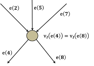
Figure 1: Example of a vertex and connecting edges

Example 1.

As an example, a local structure for a network defined above is depicted in the Figure 1, i.e. a vertex and connecting edges. The edges $\mathbf{e}\left(2\right)$, $\mathbf{e}\left(5\right)$, and $\mathbf{e}\left(7\right)$ go into the vertex and the edges $\mathbf{e}\left(4\right)$ and $\mathbf{e}\left(8\right)$ go out from the vertex. Both $\mathbf{v}_{I}\left(\mathbf{e}\left(4\right)\right)$ and $\mathbf{v}_{I}\left(\mathbf{e}\left(8\right)\right)$ indicate the vertex. At the time $t=4$, the content from $\mathbf{e}\left(2\right)$ has arrived, but the contents from $\mathbf{e}\left(5\right)$ and $\mathbf{e}\left(7\right)$ have not yet. Since $\mathbf{e}\left(1\right)$ and $\mathbf{e}\left(3\right)$, which do not appear in Figure 1, do not connect to $\mathbf{v}_{I}\left(\mathbf{e}\left(4\right)\right)$, the operation on $\mathbf{v}_{I}\left(\mathbf{e}\left(4\right)\right)$ is determined by $\theta_{4,2}$ only, and $\left\{\theta_{4,j}\right\}_{j<4}$ can be written as

$$\left\{\theta_{4,j}\right\}_{j<4}:=\left(0,\theta_{4,2},0\right).$$

Similarly, at the time $t=8$, all the contents from $\mathbf{e}\left(2\right)$, $\mathbf{e}\left(5\right)$, and $\mathbf{e}\left(7\right)$ have been received at $\mathbf{v}_{I}\left(\mathbf{e}\left(8\right)\right)$. Thus, the content sent by $\mathbf{e}\left(8\right)$ can be written as $\sum_{j<8}\theta_{8,j}Y_{j}$, where $Y_{j}$ is content received from $\mathbf{e}\left(j\right)$, and $\left\{\theta_{8,j}\right\}_{j<8}=\left(0,\theta_{8,2},0,0,\theta_{8,5},0,\theta_{8,7}\right)$.

Due to the linear structure given in (3), the random variables $Y_{j}$ is given as a linear combination of the messages $\vec{A}:=(A_{1},\cdots,A_{n})$ given in the input vertices and the shared-secure-random variables $\vec{B}:=(B_{1},\cdots,B_{n^{\prime}})$ generated at the shared-randomness vertices virtually. For simplicity, combining these random variables, we define the random vector $\vec{X}^{\prime}:=(\vec{A},\vec{B})=(X_{1}^{\prime},\cdots,X_{n+n^{\prime}}^{\prime})$. From the constants $\left\{\theta_{j,k}\right\}_{j\in\left\{1+n+l,\dots,\left|E\right|\right\},k\in\mathop{\mathbf{I}}\nolimits\left(j\right)}$, we can uniquely construct an $\mathbb{F}_{q}$-valued $(N+2n+l)\times(n+n^{\prime})$ matrix $M_{0}$ whose $(j,k)$ element is $m_{0}\left(j,k\right)$ such that

$$Y_{j}=\sum_{k=1}^{n+n^{\prime}}m_{0}\left(j,k\right)X_{k}^{\prime},$$ (4)

if there is no disturbance. The concrete construction of $M_{0}$ is given in Appendix B-A. Since $\mathbf{e}\left(j\right)$ is an output edge for $N+n+l+1\leq j\leq N+2n+l$, the corresponding elements $m_{0}\left(j,k\right)$ must satisfy

$$\left\{m_{0}\left(N+n+l+j^{\prime},k^{\prime}\right)\right\}_{k^{\prime}=1}^{n+n^{\prime}} =(\vec{0}_{j^{\prime}-1},1,\vec{0}_{n+n^{\prime}-j^{\prime}})$$ (5)

for $1\leq j^{\prime}\leq n$. Note that we use the notation $\vec{0}_{j}:=(\overbrace{0,\cdots,0}^{j})$. Rigorously writing, we can define a multiple-unicast network code by the following condition:

Definition 1.

Let $(E,V)$ be a directed network with ordered edges, $n$ and $l$ be constants which satisfies $2n+l\leq|E|$, and $I(j)$ be a map defined by Eq. (2). A network code $\left\{\theta_{j,k}\right\}_{j\in\left\{1+n+l,\dots,\left|E\right|\right\},k\in\mathop{\mathbf{I}}\nolimits\left(j\right)}$ is called a multiple-unicast network code if the coefficients $\left\{m_{0}\left(j,k\right)\right\}_{j,k}$ satisfy Eq.(5), where the coefficients $\left\{m_{0}\left(j,k\right)\right\}_{j,k}$ are defined by Eq. (4).

II-B Secrecy of classical multiple-unicast network code

In this subsection, we analyze the secrecy of the classical network code. The analysis is necessary to derive the main results regarding quantum network codes. Although there are a lot of existing works on secrecy of classical network coding [14, 16, 17, 18, 19, 20, 21, 22, 23, 24, 25, 26, 27], they don’t discuss the case when an adversary called “Eve” disturbs the contents on the part of channels as well as she wiretaps the part of channels. Only the paper [39] discusses such an adversary, though its analysis is limited to the unicast case.

II-B1 Definitions related to Eve’s attack

We define $E_{A}\subset\tilde{E}$ as the set of edges attacked by Eve, and $h$ is the size of the set, i.e., $h:=\left|E_{A}\right|$, respectively. Note that, since all the edges in the set $E\backslash\tilde{E}$ are virtual ones, Eve can’t access the edges. Eve is assumed to be able to eavesdrop and disturb the contents on all the channels in $E_{A}$. Eve also knows the network structure, i.e., the topology of network and all the coefficients $\{\theta_{j,k}\}_{j,k}$. In order to make expressions simply, we define a strictly increasing function $\varsigma\left(j\right)\in\mathbb{N}$ so that $E_{A}$ can be written as $E_{A}=\left\{\mbox{$\mathbf{e}\left(\varsigma\left(j\right)\right)$}\right\}_{j=1}^{h}$. That is, the target of the $j$-th Eve’s attack is the edge $\mathbf{e}\left(\varsigma\left(j\right)\right)$. In order to analyze such a situation, we introduce other random variables: the wiretapped random variable $Z_{j}:=Y_{\varsigma\left(j\right)}$ from the communication identified by the edge $\mathbf{e}\left(\varsigma\left(j\right)\right)$, and the injected random variable $C_{j}$ to the vertex $\mathbf{v}_{O}\left(\mathbf{e}\left(\varsigma\left(j\right)\right)\right)$ instead of $Z_{j}$. In order to simplify the following discussion, we define two random variable vectors: $\vec{C}:=(C_{1},\ldots,C_{h})$ and $\vec{X}:=(\vec{A},\vec{B},\vec{C})=(X_{1},\cdots,X_{n+n^{\prime}+h})$. Due to the linear structure of the network, there uniquely exists an $\mathbb{F}_{q}$-valued $(N+2n+l)\times(n+n^{\prime}+h)$ matrix $M$ whose $(j,k)$ element is $m\left(j,k\right)$ satisfying that the input information $Y_{j}$ of the edge $\mathbf{e}(j)$ can be expressed by

$$Y_{j}=\sum_{k=1}^{n+n^{\prime}+h}m\left(j,k\right)X_{k},$$ (6)

when the contents on the edges $E_{A}$ are disturbed by Eve. The concrete construction of $M$ is given in Appendix B-B.

When we name the received content from the edge $\mathbf{e}(j)$ as $Y_{j}^{\prime}$, the random variable can be defined as

$$Y_{j}^{\prime}:=\left\{\begin{array}[]{ll}C_{k}&\hbox{when there exists }j\hbox{ satisfying }j=\varsigma\left(k\right)\\ Y_{j}&\hbox{otherwise}.\end{array}\right.$$ (9)

We can easily define the $\mathbb{F}_{q}$-valued $(N+2n+l)\times(n+n^{\prime}+h)$ matrix $M^{\prime}$ which gives $Y_{j}^{\prime}$ from $\vec{X}$ as

$$Y_{j}^{\prime}=\sum_{k=1}^{n+n^{\prime}+h}m^{\prime}\left(j,k\right)X_{k},$$ (10)

where $m^{\prime}\left(j,k\right)$ is a $(j,k)$ elements of the matrix $M^{\prime}$. That is

$$m^{\prime}\left(j,k\right):= \left\{\begin{array}[]{ll}\delta_{k,n+n^{\prime}+j^{\prime}}&\hbox{when there exists }j^{\prime}\hbox{ satisfying }j=\varsigma\left(j^{\prime}\right)\\ m\left(j,k\right)&\hbox{otherwise}.\end{array}\right.$$ (13)

From now on, we fix the set of edges where Eve attacks, i.e. $E_{A}$, and the network code, i.e. $\{\theta_{j,k}\}_{j,k}$. That means, the matrices $M_{0}$, $M$, $M^{\prime}$, and the maps $\varsigma$, $\mathbf{e}$, $\mathbf{v}_{I}$, $\mathbf{v}_{O}$ are fixed.

II-B2 Categorization of Eve’s attack

In order to reduce complicate Eve’s attack into simple one, we categorize her attack into three types: simple attack, deterministic attack and probabilistic attack:
Simple attack: A simple attack is an attack in which Eve just deterministically chooses her injecting value $\vec{C}=\left\{X_{n+n^{\prime}+j}\right\}_{j=1}^{h}$ as a constant. Therefore, the injected value is independent from the wiretapped values $\left\{Z_{j}\right\}_{j=1}^{h}$.
Deterministic attack: A deterministic attack is defined by a set of functions $\left\{g_{j}\right\}_{j=1}^{h}$:

$$g_{j}:\mathbb{F}_{q}^{j-1}\rightarrow\mathbb{F}_{q},$$

where $g_{j}$ is not restricted to a linear function. The function $g_{j}$ gives Eve’s $j$-th injected value $C_{j}=X_{n+n^{\prime}+j}$ generated from the wiretapped variables $\{Z_{k}\}_{k=1}^{j-1}$ in her hand as

$$C_{j}=g_{j}\left(\{Z_{k}\}_{k=1}^{j-1}\right) =g_{j}\left(\left\{\sum_{k^{\prime}=1}^{n+n^{\prime}+h}m\left(\varsigma\left(k\right),k^{\prime}\right)X_{k^{\prime}}\right\}_{k=1}^{j-1}\right).$$

This attack is a special case of the causal strategy defined in the paper [39]. We write the set of all deterministic attacks as $\mathcal{G}$, i.e. all the set of $\left\{g_{j}\right\}_{j=1}^{h}$. Note that a simple attack is also a deterministic attack.

Probabilistic attack: A probabilistic attack is an attack in which Eve probabilistically chooses one of the deterministic attacks $\left\{g_{j}\right\}_{j=1}^{h}$ and applies it. Hence, a probabilistic attack is determined by a probability distribution $P_{\mathbf{G}}\left(\left\{g_{j}\right\}_{j=1}^{h}\right)$ on the set of all deterministic attacks $\mathcal{G}$, where $\mathbf{G}$ is the corresponding random variable. Note that a deterministic attack $\left\{g_{j}\right\}_{j=1}^{h}$ is a special probabilistic attack whose probability distribution satisfies $P_{\mathbf{G}}\left(\left\{g_{j}\right\}_{j=1}^{h}\right)=1$ and $P_{\mathbf{G}}\left(\left\{g^{\prime}_{j}\right\}_{j=1}^{h}\right)=0$ for any other deterministic attack $\left\{g^{\prime}_{j}\right\}_{j=1}^{h}$.

Note that, even in the case of probabilistic attack, the set of edges where Eve attacks, i.e. $E_{A}$, is fixed.

II-B3 Reduction of complex Eve’s attacks into simple ones

First, we consider the deterministic attack. In this case, any attack can be reduced to a simple attack with $\vec{C}=\vec{0}=(0,0,\cdots)$, i.e. for any deterministic attack, there is a simple attack with $\vec{C}=\vec{0}$ where Eve can get the same information with both strategies. The reason is as follows. For the original deterministic attack $\{g_{j}\}_{j=1}^{h}$, Eve’s information is given as $\left\{Z_{j}\right\}_{j=1}^{h}$. In the case of the simple attack, i.e. $\vec{C}=\vec{0}$, we denote Eve’s information by $\left\{\tilde{Z}_{j}\right\}_{j=1}^{h}$ . Due to the linearity of the network, we have

$$Z_{j}=\tilde{Z}_{j}+\sum_{k=1}^{h}m(\varsigma\left(j\right),n+n^{\prime}+k)g_{k}(\left\{Z_{k^{\prime}}\right\}_{k^{\prime}=1}^{k-1}),$$ (14)

for $1\leq j\leq h$. As you can check, all the elements $m(j,k)$ are defined by the network code and the set of edges where Eve attacks. This fact guarantees that we can solve the eq. (14) with respect to $\{Z_{k}\}_{k=1}^{j}$. This fact can be rewritten as the following lemma.

Lemma 1 ([39, Theorem 1]).

Any deterministic attack can be reduced to a simple attack with $\vec{C}=\vec{0}_{h}$. Since any probabilistic attack is given as a probabilistic mixture of deterministic attacks, it can also be reduced to the simple attack with $\vec{C}=\vec{0}_{h}$.

For reader’s convenience, we summarize all the random variables we defined in Table II

TABLE II: Random variables of the network coding.

$A_{j}$	The random variable of the $j$-th message
$B_{j}$	The random variable of the $j$-th shared number
$C_{j}$	The random variable injected at the end of edge $\mathbf{e}(\varsigma\left(j\right))$
$X_{j}$	An alias of the variable $A_{j}$, $B_{j-n}$, or $C_{j-n-n^{\prime}}$
$Y_{j}$	The random variable inputted to the edge $\mathbf{e}(j)$
$Y_{j}^{\prime}$	The random variable outputted from the edge $\mathbf{e}(j)$
$Z_{j}$	The random variable wiretapped at the edge $\mathbf{e}(\varsigma\left(j\right))$
$\tilde{Z}_{j}$	The random variable wiretapped at the edge $\mathbf{e}(\varsigma\left(j\right))$ under the virtual condition $\vec{C}=\vec{0}_{h}$

II-B4 Security analysis for Eve’s attack on $E_{A}$

For given $E_{A}$ and the function $\varsigma$, we define a $h\times\left(n+n^{\prime}+h\right)$ matrix $M_{\varsigma}$ whose elements are given by $\left\{m\left(\varsigma\left(j\right),k\right)\right\}_{1\leq j\leq h,1\leq k\leq n+n^{\prime}+h}$. We further define submatrices of $M_{\varsigma}$ as $M_{\varsigma}=\left(M_{\varsigma,1},M_{\varsigma,2},M_{\varsigma,3}\right)$ where the sizes of $M_{\varsigma,1}$, $M_{\varsigma,2}$, and $M_{\varsigma,3}$ are $h\times n$, $h\times n^{\prime}$, and $h\times h$, respectively. For $\vec{x}=\left(\vec{a},\vec{b},\vec{c}\right)\in\mathbb{F}_{q}^{n+n^{\prime}+h}$, the condition

$$z_{j}=\sum_{k=1}^{n+n^{\prime}+h}m_{\varsigma}\left(j,k\right)x_{k}$$ (15)

can be rewritten as

$$\vec{z}=M_{\varsigma,1}\vec{a}+M_{\varsigma,2}\vec{b}+M_{\varsigma,3}\vec{c}.$$ (16)

Lemma 2.

Secrecy holds for Eve’s attack on $E_{A}$ if and only if the following condition holds: For any vector $\vec{a}\in\mathbb{F}_{q}^{n}$, there exists a function $\vec{\mathfrak{b}}(\vec{a})\in\mathbb{F}_{q}^{n^{\prime}}$ such that

$$M_{\varsigma,1}\vec{a}=M_{\varsigma,2}\vec{\mathfrak{b}}(\vec{a}).$$ (17)

The condition is trivially equivalent to the condition that the image of $M_{\varsigma,1}$ is contained in that of $M_{\varsigma,2}$.

Proof.

Due to Lemma 1, it is enough to discuss the case with $\vec{C}=\vec{0}$. When secrecy holds, $\{M_{\varsigma,2}\vec{b}|\vec{b}\in\mathbb{F}_{q}^{n^{\prime}}\}=\{M_{\varsigma,1}\vec{a}+M_{\varsigma,2}\vec{b}|\vec{b}\in\mathbb{F}_{q}^{n^{\prime}}\}$ for any $\vec{a}\in\mathbb{F}_{q}^{n}$. The latter set contains $M_{\varsigma,1}\vec{a}$, which ensures the existence of $\vec{\mathfrak{b}}(\vec{a})$. When such a function $\vec{\mathfrak{b}}(\vec{a})$ exists, the distribution of $M_{\varsigma,2}\vec{B}$ is the same as that of $M_{\varsigma,1}\vec{a}+M_{\varsigma,2}\vec{B}$. That is because the variable $\vec{B}$ is uniformly distributed. This fact implies the secrecy. ∎

II-C Recoverability against Eve’s attack

For our analysis of deriving quantum network coding, we need to introduce the concept of recoverability of the classical network code against Eve’s attack in addition to the secrecy. The concept of recoverability is defined as follows. We consider the situation that Eve can disturb contents on the channels in $E_{A}$ as is done in the case of secrecy analysis. In other words, she can inject any contents on the channels in $E_{A}$. In such a situation, we imagine a receiver Bob who can use all the received contents of the the channel identified by a set $E_{P}\subset E\backslash E_{R}$. For convenience, we give a name “protected edges” to the edges in $E_{P}$. He can additionally access all the shared-random variables, and can know the set $E_{A}$ and the network structure, i.e. the matrix $M^{\prime}$. However, Bob does not know what content is injected in the channel in the set $E_{A}$, if the channel is not in the set $E_{P}$. In this case, if Bob can reconstruct the original messages, we call that the messages is recoverable from Eve’s attack by the protected edges $E_{P}$. We will require the recoverability by a certain subset $E_{P}$ for the security of a deriving quantum network code.

TABLE III: Sets of edges of the network coding.

$\tilde{E}$	The set of edges which express actual channels
$E_{I}$	The set of input edges connected from input vertices
$E_{O}$	The set of output edges connected to output vertices
$E_{R}$	The set of shared-randomness edges connected from shared-randomness vertices
$E$	The union of the sets $\tilde{E}$, $E_{I}$, $E_{O}$, and $E_{R}$
$E_{P}$	The set of protected edges
$E_{A}$	The set of edges attacked by Eve

Now, we give more rigid definition of the concept of the recoverability. For the subset $E_{P}$, we define the strictly increasing function $\iota:\ \left\{1,\cdots,\left|E_{P}\right|\right\}\rightarrow\left\{1,\cdots,n,n+l+1,\cdots,N+2n+l\right\}$ which satisfies $E_{P}=\left\{\mathbf{e}\left(\iota\left(j\right)\right)\right\}_{j=1}^{h^{\prime}}$, where $h^{\prime}:=\left|E_{P}\right|$. Then, the contents $\left\{Y^{\prime}_{\iota\left(j\right)}\right\}_{j=1}^{h^{\prime}}$ received from the protected edges $E_{P}$ can be written as

$$Y^{\prime}_{\iota\left(j\right)}=\sum_{k=1}^{n+n^{\prime}+h}m_{\iota}^{\prime}\left(j,k\right)X_{k},$$ (18)

where $m_{\iota}^{\prime}\left(j,k\right):=m^{\prime}\left(\iota\left(j\right),k\right)$ is a matrix elements of the $h^{\prime}\times(n+n^{\prime}+h)$ matrix $M^{\prime}_{\iota}$. Then, we rigidly define the concept of the recoverability as follows.

Definition 2.

We call that the messages are recoverable for Eve’s attack on $E_{A}$ by a subset $E_{P}$, when for any vector $\vec{b}\in\mathbb{F}_{q}^{n^{\prime}}$, there exists a function $f_{\vec{b}}:\ \mathbb{F}_{q}^{h^{\prime}}\rightarrow\mathbb{F}_{q}^{n}$ such that

$$f_{\vec{b}}\left(M_{\iota}^{\prime}\cdot(\vec{a},\vec{b},\vec{c})^{T}\right)=\vec{a}$$ (19)

for any $\vec{a}\in\mathbb{F}_{q}^{n}$ and $\vec{c}\in\mathbb{F}_{q}^{h}$.

Here, $T$ means the transposition. Note that the matrix $M_{\iota}^{\prime}$ is uniquely given only from the matrix $M_{0}$ and the sets $E_{A}$ and $E_{P}$.

The function $f_{\vec{b}}$ is nothing but a decoder of the messages $\vec{A}$ from the contents received from $E_{P}$. The function depends on $M_{\iota}^{\prime}$ and $\vec{b}$ only. Since condition (19) does not depend on the choice of $\vec{c}$, it guarantees the recoverability even when Eve chooses $\vec{C}$ depending on her wiretapped variable.

Notice that this kind of recoverability does not imply the recoverability of the messages by terminal nodes, and we don’t assume the condition $E_{P}\cap E_{A}=\emptyset$. In other words, a channel corresponding to a “protected” edge may be disturbed by Eve. Therefore, at the channel in $E_{P}\cap E_{A}$, Eve can completely control the information obtained by Bob.

It is informative to show a toy example of a classical network code in which the contents from the edges in $E_{P}\cap E_{A}$ are useful to recover the messages. The example is as follows. A single message $A_{1}$ is transfer from $s_{1}$ to $t_{1}$ via two channels $\mathbf{e}(2)$ and $\mathbf{e}(3)$ simultaneously. There is no randomness. The terminal node $t_{1}$ sums up the two received contents and obtains recovered message by dividing it by $2$. $\mathbf{e}(1)$ and $\mathbf{e}(4)$ are the input edge and output edge respectively. We define the set $E_{P}$ to be $\{\mathbf{e}(3),\mathbf{e}(4)\}$, and consider the case $E_{A}=\{\mathbf{e}(3)\}$. In this case, we can give

$$M^{\prime}_{\iota}=\left(\begin{array}[]{cc}0&1\\ 2^{-1}&2^{-1}\end{array}\right),$$ (20)

and we know that $\vec{A}\in\mathbb{F}_{q}^{1}$ and $\vec{C}\in\mathbb{F}_{q}^{1}$. Therefore, by selecting the function $f_{\vec{b}}(\vec{y})$ as $2y_{2}-y_{1}$, we can check that the message is recoverable for Eve’s attack on $E_{A}=\{\mathbf{e}(3)\}$, though this network code isn’t secure against Eve’s attack on $E_{A}$. The necessity of the content from the channel $\mathbf{e}(3)\in E_{P}\cap E_{A}$ is checked from the fact that the coefficient of $y_{1}$ for the function $f_{\vec{b}}(\vec{y})$ is not 0.

In the end of this section, the defined matrices in this section are summarized in Table IV.

TABLE IV: Summary of matrices

matrix	input system	output system	equation
$M_{0}$	messages, shared random variables	inputs of all edges	(4)
		$=$ outputs of all edges
$M$	messages, shared random variables,	inputs of all edges	(6)
	Eve’s input
$M^{\prime}$	messages, shared random variables,	outputs of all edges	(13)
	Eve’s input
$M_{\varsigma}$	messages, shared random variables,	inputs of attacked edges	(15)
	Eve’s input
$M_{\iota}^{\prime}$	messages, shared random variables,	outputs of protected edges	(18)
	Eve’s input

III Secure quantum network coding for general network

III-A Coding scheme

In this section, we derive a quantum network code from a linear classical network code, and analyze the security of the quantum network coding based on the properties of the original classical network coding which are discussed in the previous section. Quantum network coding can be categorized by the type of classical communication allowed [5, 6, 8, 9, 10, 11]. In this paper, we consider the case that any authenticated public classical communication from any nodes to the terminal nodes is freely available, and all the communication may be eavesdropped by Eve. In this case, it is known that, for an arbitrary classical multiple-unicast code on an arbitrary classical network, there exists a corresponding quantum multiple-unicast network code on the corresponding quantum network [10, 11]. We start this subsection by extending this known result to the case when shared randomness is employed.

III-A1 The notations defined from the original classical network coding

In the following, we fixed the original classical network code. As is done in the previous section, from the classical network code, we define integers $N$, $n$, $n^{\prime}$, $l$, $q$, $\{l_{k}\}_{k=1}^{n^{\prime}}$, sets $\tilde{V}$, $V_{S}$, $V_{T}$, $E$, $\tilde{E}$, $E_{I}$, $E_{O}$, $E_{R}$, $E_{P}$, maps $\mathbf{e}$, $\mathbf{v}_{I}$, $\mathbf{v}_{O}$, $\mathop{\mathbf{I}}\nolimits$, and the coefficients $\left\{\theta_{j,k}\right\}_{j\in\left\{n+l+1,\cdots,|E|\right\},k\in\mathop{\mathbf{I}}\nolimits\left(j\right)}$, which identify the matrix $M_{0}$ and its elements $m_{0}(j,k)$ by Eq.(4).

Other than the above notations, we have to define additional notation of a map $\mathfrak{E}$ from the element in $E$ to the subset of $V_{T}$ such that

$$\mathfrak{E}(\mathbf{e}^{\prime}):= \{\mathbf{v}_{I}(\mathbf{e}(N+n+l+j))|1\leq j\leq n\land\exists k,\;(\mathbf{e}^{\prime}=\mathbf{e}(k)\land m_{0}(k,j)\neq 0)\}.$$ (21)

Note that, when the content tranferred by the edge $\mathbf{e}^{\prime}$ depends on some messages, the set $\mathfrak{E}(\mathbf{e}^{\prime})$ indicates that of all the terminal nodes where the messages are reconstructed.

III-A2 Considering situation of the quantum network

From the items defined above, we list the conditions of the considering situation as a quantum network:

• The number of nodes of the quantum network coding is $N$, and each member is labelled by an element of $\tilde{V}$ individually.

• The total Hilbert space, which all the nodes treat, is the direct product of the subspaces $\mathcal{H}_{j}$ for $1\leq j\leq n$ or $n+l<j\leq N+2n+l$. Every subspace $\mathcal{H}_{j}$ is made from a $q$-dimensional Hilbert space, and has a computational basis $\left\{\left|k\right\rangle_{j}\right\}_{k\in\mathbb{F}_{q}}$. Every subspace $\mathcal{H}_{j}$ of the first $n$ subspaces is occupied by the node $\mathbf{v}_{O}\left(\mathbf{e}\left(j\right)\right)$ for each $j$. Every subspace $\mathcal{H}_{j}$ of the other subspaces is occupied by the node $\mathbf{v}_{I}\left(\mathbf{e}\left(j\right)\right)$ for each $j$.

• Initially, there is no correlation, especially no entanglement, between any pair of nodes except for the preshared quantum messages.

• At the time $t=j$, we can use a quantum channel identified by $\mathbf{e}\left(j\right)$ which transfers the quantum subspace $\mathcal{H}_{j}$ from the node $\mathbf{v}_{I}\left(\mathbf{e}\left(j\right)\right)$ to the node $\mathbf{v}_{O}\left(\mathbf{e}\left(j\right)\right)$ where $n+l<j\leq N+n+l$. Any channel can be used only once, and any channel is an identity channel if the eavesdropper Eve does not attack the channel.

• A random number $b_{j}\in\mathbb{F}_{q}$, which is secret from Eve, is sheared by the nodes $\mathbf{v}_{O}\left(\mathbf{e}\left(k\right)\right)$ for $n+\sum_{j^{\prime}=1}^{j-1}l_{j^{\prime}}<k\leq n+\sum_{j^{\prime}=1}^{j}l_{j^{\prime}}$ initially where $1\leq j\leq n^{\prime}$. Other than the random numbers, the vertex $\mathbf{v}_{O}\left(\mathbf{e}\right)$ shares a secret random number in $\mathbb{F}_{q}$ with all vertices in $\mathfrak{E}(\mathbf{e})$ for every $\mathbf{e}\in E_{P}$.

• Any node can apply any unitary operations and measurements for the occupied quantum subspaces depending on any classical information which the node has at any time.

• Any authenticated but public classical communication is freely available from any node to all of the terminal nodes. That is, each node can freely send classical information to any terminal node, and the information may be revealed to Eve.

III-A3 Purpose of the quantum network coding

There are two purposes for the multiple-unicast quantum network code. The first purpose is to send an arbitrary quantum state on $\mathbb{C}^{q}$ from a source node $\mathbf{v}_{O}\left(\mathbf{e}\left(j\right)\right)$ to a terminal node $\mathbf{v}_{I}\left(\mathbf{e}\left(N+n+l+j\right)\right)$ for all $j\in\{1,2,\cdots,n\}$ through the quantum network simultaneously. We call the state a quantum message. Since any classical communication to terminal nodes is free, this task is equivalent to constructing the maximally entangled state between a $q$-dimensional subspace in a source node $\mathbf{v}_{O}\left(\mathbf{e}\left(j\right)\right)$ and that in a terminal node $\mathbf{v}_{I}\left(\mathbf{e}\left(N+n+l+j\right)\right)$ for all $j\in\{1,2,\cdots,n\}$. Second purpose is to prevent the leakage of any information about the quantum messages to Eve where she can access all the information transmitted via public classical channel and quantum states as contents on the restricted quantum channels identified by $E_{A}$.

In this paper, we will show some examples of quantum network codes which satisfies the following two properties. First, quantum messages can be sent with fidelity 1, if there is no disturbance for any channels. Second, even if any one or two edges are completely controlled by Eve, i.e. the transmitted contents are completely stolen and other contents are injected on any one or two edges in $\tilde{E}$, it can be guaranteed that Eve can get no information about the quantum messages.

III-A4 Preliminary definition of the quantum network coding

Before presenting the quantum network code, we give the notations used in it. For a subset $D$ of $\{1,\cdots,N+2n+l\}$, we define the subspace ${\mathcal{H}}_{D}:=\bigotimes_{j\in D}{\mathcal{H}}_{j}$. For an $\mathbb{F}_{q}$-valued vector $\vec{y}=\left(y_{1},\cdots,y_{N+2n+l}\right)\in\mathbb{F}_{q}^{N+2n+l}$, we abbreviate the state $\bigotimes_{j\in D}\left|y_{j}\right\rangle_{j}$ as $\left|\vec{y}\right\rangle_{D}$. Note that, from this definition, a single vector has multiple expressions in order to simplify the expressions hereafter. To distinguish a classical system from a quantum one easily, we introduce sets

$$\mathop{\mathbf{QI}}\nolimits\left(j\right) :=\left\{k\in\mathop{\mathbf{I}}\nolimits\left(j\right)|1\leq k\leq n\;\lor\;n+l<k\right\}$$

$$\mathop{\mathbf{CI}}\nolimits\left(j\right) :=\left\{k\in\mathop{\mathbf{I}}\nolimits\left(j\right)|n<k\leq n+l\right\},$$

where $\mathop{\mathbf{I}}\nolimits\left(j\right)$ is defined by Eq.(2). Using these notations, depending on the matrix $\theta=\left\{\theta_{j,k}\right\}_{j,k}$, we define the controlled unitary operation $U_{j}(\theta)$ acting on the Hilbert space ${\mathcal{H}}_{j}\otimes{\mathcal{H}}_{\mathop{\mathbf{QI}}\nolimits\left(j\right)}$ as

$$U_{j}(\theta) = q^{-N-2n-l+1+|\mathop{\mathbf{QI}}\nolimits\left(j\right)|}\sum_{\vec{y}\in\mathbb{F}_{q}^{N+2n+l}}|y_{j}+\sum_{k\in\mathop{\mathbf{QI}}\nolimits\left(j\right)}\theta_{j,k}y_{k}\rangle_{j}\left\langle y_{j}\right|_{j}\otimes\left|\vec{y}\right\rangle_{\mathop{\mathbf{QI}}\nolimits(j)}\left\langle\vec{y}\right|_{\mathop{\mathbf{QI}}\nolimits(j)}.$$

On the space ${\mathcal{H}}_{j}$, whose computational basis is $\{\left|y\right\rangle_{j}\}_{y\in\mathbb{F}_{q}}$, we introduce the Fourier basis $\{|\tilde{\beta}\rangle_{j}\}_{\beta\in\mathbb{F}_{q}}$ as

$$|\tilde{\beta}\rangle_{j}:=q^{-1/2}\sum_{y\in\mathbb{F}_{q}}\omega^{\mathop{\rm tr}\nolimits y\beta}\left|y\right\rangle_{j},$$

where $\omega:=\exp\left(-\frac{2\pi i}{p}\right)$. Here, $\mathop{\rm tr}\nolimits z$ expresses the element $\mathop{\rm Tr}\nolimits\psi(z)\in\mathbb{F}_{p}$, where $\psi(z)$ denotes the matrix representation of the multiplication map $x\mapsto zx$ which identifies the finite field $\mathbb{F}_{q}$ with the vector space $\mathbb{F}_{p}^{d}$, where $d$ is the degree of algebraic extension of $\mathbb{F}_{q}$, i.e. $p^{d}=q$. For the details, see [40, Section 8.1.2]. We also define the generalized Pauli operators $\mathsf{X}_{j}(x)$ and $\mathsf{Z}_{j}(\beta)$ as $\mathsf{X}_{j}(x):=\sum_{y\in\mathbb{F}_{q}}\left|y+x\right\rangle_{j}\left\langle y\right|_{j}$ and $\mathsf{Z}_{j}(\beta):=\sum_{y\in\mathbb{F}_{q}}\omega^{\mathop{\rm tr}\nolimits y\beta}\left|y\right\rangle_{j}\left\langle y\right|_{j}$.

III-A5 Quantum network code

Using the notations defined above, we show the multi-unicast quantum network code which transfers the quantum messages from the space $\bigotimes_{j=1}^{n}\mathcal{H}_{j}$ into the space $\bigotimes_{j=1}^{n}\mathcal{H}_{N+n+l+j}$.

Protocol 1 The quantum network code deriving from a general classical linear network code

0:  Initialization First, all the spaces $\mathcal{H}_{j}$ are initialized to the state $\left|0\right\rangle_{j}$ for $n+l<j\leq N+2n+l$, at each edge.

0:  Transmission This step consists of $N+n$ substeps. The $j$-th substeps can be described as follows. At the time $t=j^{\prime}:=n+l+j$, the node $\mathbf{v}_{I}\left(\mathbf{e}\left(j^{\prime}\right)\right)$ operates the unitary

$$\mathsf{X}_{j^{\prime}}(\sum_{k\in\mathop{\mathbf{CI}}\nolimits\left(j^{\prime}\right)}\theta_{j^{\prime},n+k}b_{k})U_{j^{\prime}}\left(\theta\right)$$ (22)

on ${\mathcal{H}}_{j^{\prime}}\otimes{\mathcal{H}}_{\mathop{\mathbf{QI}}\nolimits\left(j^{\prime}\right)}$ where ${\mathcal{H}}_{j^{\prime}}$ is the controlled system and ${\mathcal{H}}_{\mathop{\mathbf{QI}}\nolimits\left(j^{\prime}\right)}$ is the controlling system. If $j\leq N$, the node $\mathbf{v}_{I}\left(\mathbf{e}\left(j^{\prime}\right)\right)$ sends the Hilbert space ${\mathcal{H}}_{j^{\prime}}$ to the node $\mathbf{v}_{O}\left(\mathbf{e}\left(j^{\prime}\right)\right)$ via the quantum channel $\mathbf{e}\left(j^{\prime}\right)$. Note that, if the node $\mathbf{v}_{I}\left(\mathbf{e}\left(j^{\prime}\right)\right)$ does not share any random number, i.e. $\mathop{\mathbf{CI}}\nolimits\left(j^{\prime}\right)=\emptyset$, the generalized Pauli operator $\mathsf{X}_{j^{\prime}}(\cdot)$ in the above relation is considered to be the identity operator.

0:  Measurement on Fourier-basis This step consists of $N+n$ substeps. The step identified by $j\in\{1,\cdots,n,n+l+1,\cdots N+n+l\}=:G^{\prime}$ can be described as follows. The node $\mathbf{v}_{O}\left(\mathbf{e}\left(j\right)\right)$ measures the Hilbert space ${\mathcal{H}}_{j}$ in the Fourier basis, and sends the measurement outcome $\beta_{j}$ to all the terminal nodes in $\mathfrak{E}(\mathbf{e}\left(j\right))$. Here, if $\mathbf{e}\left(j\right)\notin E_{P}$, the outcome is sent by public channel, i.e. the outcome may eavesdropped by Eve, and, if $\mathbf{e}\left(j\right)\in E_{P}$, the outcome is sent by the one-time pad, i.e. a secret randomness shared with the vertices in $\mathfrak{E}(\mathbf{e}\left(j\right))$ is consumed and the outcome is completely secret from Eve.

0:  Recovery For all $j$ satisfying $1\leq j\leq n$, the terminal node $\mathbf{v}_{I}\left(\mathbf{e}\left(N+n+l+j\right)\right)$ operates $\mathsf{Z}_{N+n+l+j}\left(\sum_{k\in G^{\prime}}\beta_{k}m_{0}\left(k,j\right)\right)$, where a matrix $M_{0}$ is defined by Eq.(4).

Note that, for all public communications sending an outcome $\beta_{j}$ to multiple nodes at a substep in Step 3, we can combine a common single secret randomness for the one-time pad without losing secrecy. Furthermore, there is a special case such that $\mathfrak{E}(\mathbf{e}(j))$ contains only the single node $\mathbf{v}_{O}(\mathbf{e}(j))$. In that case, we send the outcome to the node $\mathbf{v}_{O}(\mathbf{e}(j))$ where the outcome is obtained. Therefore, the procedure is equivalent to doing nothing. As a result, we don’t have to use any shared randomness even if $\mathbf{e}(j)\in E_{P}$ for such a situation.

As you have seen, our protocol depends only on the set of coefficients $\{\theta_{j,k}\}_{j,k}$ and the set of protected edges $E_{P}$. That is, our protocol is uniquely determined by the pair of $\{\theta_{j,k}\}_{j,k}$ and $E_{P}$, and we call it the quantum network code $\left\{\theta_{jk}\right\}_{j\in\left\{n+l+1,\cdots,|E|\right\},k\in\mathop{\mathbf{I}}\nolimits\left(j\right)}$ with the set of protected edges $E_{P}$.

III-B Validity analysis

In order to analyze the quantum network coding, it is convenient to introduce ancillary set of $q$-dimensional Hilbert spaces ${\mathcal{H}}_{j-n}$ occupied by the source node $\mathbf{v}_{O}\left(\mathbf{e}\left(j\right)\right)$ for $1\leq j\leq n$. Note that we never perform any operations on the ancillary spaces.

As a generalization of [10, Theorem 1], we obtain the following theorem.

Theorem 1.

Suppose that the corresponding classical network coding identified by $\{\theta_{j,k}\}_{j,k}$ is a multi-unicast network code. By Protocol 1, any quantum message on the space $\mathcal{H}_{j}$ are simultaneously transferred to the space $\mathcal{H}_{N+n+l+j}$ with fidelity $1$ for any $j$ satisfying $1\leq j\leq n$ if no one disturbs the protocol. That is, when the maximally entangled state $q^{-1/2}\sum_{x\in\mathbb{F}_{q}}\left|x\right\rangle_{j-n}\left|x\right\rangle_{j}\in{{\mathcal{H}}_{j-n}\otimes\mathcal{H}}_{j}$ is prepared as the initial state on every source node $\mathbf{v}_{O}\left(\mathbf{e}\left(j\right)\right)$ for $1\leq j\leq n$, Protocol 1 makes the resultant state to be a maximally entangled state $q^{-1/2}\sum_{x\in\mathbb{F}_{q}}\left|x\right\rangle_{j-n}\left|x\right\rangle_{N+n+l+j}$ on ${\mathcal{H}}_{j-n}\otimes{\mathcal{H}}_{N+n+l+j}$ for any $j$ satisfying $1\leq j\leq n$ if all the quantum channels are identity channels.

Remember that the transmission of quantum states is mathematically equivalent to sharing the maximally entangled state between the input and output systems.

Proof.

We define the Hilbert spaces ${\mathcal{H}}_{I}$ and ${\mathcal{H}}_{O}$, as ${\mathcal{H}}_{I}:=\bigotimes_{j=1}^{n}{\mathcal{H}}_{j-n}$ and ${\mathcal{H}}_{O}:=\bigotimes_{j=1}^{n}{\mathcal{H}}_{N+n+l+j}$ respectively. Their bases $\{\bigotimes_{j=1}^{n}\left|a_{j}\right\rangle_{j-n}\}$ and $\{\bigotimes_{j=1}^{n}\left|a_{j}\right\rangle_{N+n+l+j}\}$ are abbreviated as $\{\left|\vec{a}\right\rangle_{I}\}$ and $\{\left|\vec{a}\right\rangle_{O}\}$. The sets $G$ and $G^{\prime}$ are defined to be $\{1,\cdots,n,n+l+1,\cdots,N+2n+l\}$ and $\{1,\cdots,n,n+l+1,\cdots,N+n+l\}$. By straightforward calculation, we find that the density matrix on the network after Step 2 is

$$\frac{1}{q^{n+n^{\prime}}}\sum_{\vec{b}\in\mathbb{F}_{q}^{n^{\prime}}}\sum_{\vec{a},\vec{a}^{\prime}\in\mathbb{F}_{q}^{n}}\left|\vec{a}\right\rangle_{I}\left\langle\vec{a}^{\prime}\right|_{I}\otimes\left|M_{0}\cdot(\vec{a},\vec{b})^{T}\right\rangle_{G}\left\langle M_{0}\cdot(\vec{a}^{\prime},\vec{b})^{T}\right|_{G}$$

$$= \frac{1}{q^{n+n^{\prime}}}\sum_{\vec{b}\in\mathbb{F}_{q}^{n^{\prime}}}\sum_{\vec{a},\vec{a}^{\prime}\in\mathbb{F}_{q}^{n}}\left|\vec{a}\right\rangle_{I}\left\langle\vec{a}^{\prime}\right|_{I}\otimes\left|M_{0}\cdot(\vec{a},\vec{b})^{T}\right\rangle_{G^{\prime}}\left\langle M_{0}\cdot(\vec{a}^{\prime},\vec{b})^{T}\right|_{G^{\prime}}\otimes\left|\vec{a}\right\rangle_{O}\left\langle\vec{a}^{\prime}\right|_{O},$$

if all the quantum channels are identity channels. At the equality, we use the assumption that the classical protocol is a multiple-unicast network code. The state after Step 3 can be expressed as

$$\frac{1}{q^{n}}\sum_{\vec{a},\vec{a}^{\prime}\in\mathbb{F}_{q}^{n}}\omega^{\mathop{\rm tr}\nolimits\vec{\beta}_{G^{\prime}}^{T}\cdot M_{0}\cdot\left(\vec{a}^{\prime}-\vec{a},\vec{0}_{n^{\prime}}\right)^{T}}\left|\vec{a}\right\rangle_{I}\left\langle\vec{a}^{\prime}\right|_{I}\otimes\left|\vec{a}\right\rangle_{O}\left\langle\vec{a}^{\prime}\right|_{O},$$

where $\vec{\beta}_{G^{\prime}}:=(\beta_{1},\cdots,\beta_{n},\vec{0}_{l},\beta_{n+l+1},\cdots,\beta_{N+n+l},\vec{0}_{n})^{T}$. Finally, the state after Step 4 can be written as

$$\frac{1}{q^{n}}\sum_{\vec{a},\vec{a}^{\prime}\in\mathbb{F}_{q}^{n}}\left|\vec{a}\right\rangle_{I}\left\langle\vec{a}^{\prime}\right|_{I}\otimes\left|\vec{a}\right\rangle_{O}\left\langle\vec{a}^{\prime}\right|_{O},$$

which is the maximally entangled state to be constructed in this protocol. ∎

III-C Security analysis

Next, we discuss the security of the transmitted quantum state under the following four assumptions. First, the eavesdropper Eve can eavesdrop and modify the contents transmitted via all the channels in $E_{A}$, which is a subset of $\tilde{E}$. Second, she also knows the network structure, i.e., the topology of the network and all the coefficients $\{\theta_{j,k}\}_{j,k}$. Third, Eve can get any information transmitted by the public channel. Finally, Eve can’t obtain any other information which may be correlated to the quantum messages.

In order to treat Eve’s attack formally, we introduce the map $\varsigma$ and the constant $h$ defined from $\mathbf{e}$ and $E_{A}$ as is done in the case of Eve’s attack for the classical network coding. Using this notation, we formulate the Eve’s attack as follow.

Eve’s attack: Eve initially occupies her initial Hilbert space $\mathcal{W}$ with a state $|\phi_{ini}\rangle$, where the dimension of the space $\mathcal{W}$ is chosen to be sufficiently large so that every Eve’s operations can be treated as a unitary operation. At the time $t=\varsigma\left(j\right)$, Eve applies the unitary $W_{j}$ on ${\mathcal{H}}_{\varsigma\left(j\right)}\otimes{\mathcal{W}}$ for $1\leq j\leq h$. Note that $W_{j}$ does not depend on the outcomes $\{\beta_{k}\}_{k}$ since the measurement step is done just after the transmission step. However, Eve may finally get the measurement outcomes $\beta_{k}$ where $1\leq k\leq n$ or $n+l<k\leq N+n+l$ and $\forall j,\;k\neq\iota(j)$, i.e. the measurement outcomes of the contents received from non-protected edge. In the following security analysis, these classical information is denoted by a diagonalized density matrix on the space $\mathcal{V}$, where the initial state of $\mathcal{V}$ is a pure state.

From this assumption, we also formulate the security of the quantum network coding against Eve’s attack:

Definition 3.

The quantum network code $\left\{\theta_{j,k}\right\}_{j\in\left\{n+l+1,\cdots,|E|\right\},k\in\mathop{\mathbf{I}}\nolimits\left(j\right)}$ with the set of protected edges $E_{P}$ is called secure for Eve’s attack $\{V_{j}\}_{j}$ on the set of edges $E_{A}$ if the following condition holds. When the initial state on the Hilbert space $\mathcal{H}_{I}\otimes\bigotimes_{j=1}^{n}\mathcal{H}_{j}$ is the maximally entangled state between $\mathcal{H}_{I}$ and $\bigotimes_{j=1}^{n}\mathcal{H}_{j}$ i.e. the initial state is that used in Theorem 1, the final state of the protocol on the subspace $\mathcal{H}_{I}\otimes\mathcal{W}\otimes\mathcal{V}$ is a product state with respect to the partition between $\mathcal{H}_{I}$ and $\mathcal{W}\otimes\mathcal{V}$.

It is easily understood that: this defined condition of the security is equivalent to the condition that there is no leakage of the information about the quantum messages by the quantum network code. Note that, we call the state $\rho\in\mathfrak{B}\left({\mathcal{H}}^{\prime}\otimes{\mathcal{H}}^{\prime\prime}\right)$ a product state if there exist $\rho^{\prime}\in\mathfrak{B}\left({\mathcal{H}}^{\prime}\right)$ and $\rho^{\prime\prime}\in\mathfrak{B}\left({\mathcal{H}}^{\prime\prime}\right)$ such that $\rho=\rho^{\prime}\otimes\rho^{\prime\prime}$. Now, we can present the main result of this paper:

Theorem 2.

The quantum network code $\left\{\theta_{j,k}\right\}_{j\in\left\{n+l+1,\cdots,|E|\right\},k\in\mathop{\mathbf{I}}\nolimits\left(j\right)}$ with the set of protected edges $E_{P}$ is secure for all Eve’s attacks on the set of edges $E_{A}$ if the following two conditions hold. (i) The classical network code $\left\{\theta_{j,k}\right\}_{j\in\left\{n+l+1,\cdots,|E|\right\},k\in\mathop{\mathbf{I}}\nolimits\left(j\right)}$ is secure for Eve’s attacks on the set of edges $E_{A}$. (ii) The messages are recoverable for Eve’s attack on $E_{A}$ by the set of protected edges $E_{P}$ in the sense of the classical network coding.

From this theorem, we know that the security for the quantum messages is related not only to the secrecy of the classical information but also to the recoverability of the classical information. Strictly speaking, this theorem guarantees that the security analysis of our quantum network coding is reduced to the analysis of the secrecy and the recoverability of the corresponding classical network coding.

III-D Security proof

We can prove Theorem 2 by checking Definition 2 directly as follows:

Proof of Theorem 2:

We consider the case that we initialize the state on the Hilbert space $\mathcal{H}_{I}\otimes\bigotimes_{j=1}^{n}\mathcal{H}_{j}$ to be the maximally entangled state between $\mathcal{H}_{I}$ and $\bigotimes_{j=1}^{n}\mathcal{H}_{j}$, i.e. $\bigotimes_{j=1}^{n}q^{-1/2}\sum_{a\in\mathbb{F}_{q}}\left|a\right\rangle_{j-n}\left|a\right\rangle_{j}$, and execute Protocol 1.

Given Eve’s attack $\{V_{j}\}$ on the set of edges $E_{A}$, the total density matrix $\rho$ on the space $\mathcal{H}_{I}\otimes\mathcal{H}_{O}\otimes\mathcal{V}^{\prime}\otimes\mathcal{W}\otimes\mathcal{V}$ becomes

$$q^{-2n-n^{\prime}-l}\sum_{\vec{a},\vec{a}^{\prime}\in\mathbb{F}_{q}^{n}}\sum_{\vec{b}\in\mathbb{F}_{q}^{n^{\prime}}}\sum_{\vec{c},\vec{c}^{\prime}\in\mathbb{F}_{q}^{h}}\sum_{\vec{\beta}\in\mathbb{F}_{q}^{N+2n+l}}\left|\vec{a}\right\rangle_{I}\left\langle\vec{a}^{\prime}\right|_{I}$$

$$\otimes\langle\tilde{\vec{\beta}}|_{G^{\prime}}|M^{\prime}(\vec{a},\vec{b},\vec{c})^{T}\rangle_{G}\langle M^{\prime}(\vec{a}^{\prime},\vec{b},\vec{c}^{\prime})^{T}|_{G}|\tilde{\vec{\beta}}\rangle_{G^{\prime}}\otimes\bigotimes_{j\in G^{\prime}}\left|\beta_{j}\right\rangle_{j}^{\mathcal{V}^{\prime}}\left\langle\beta_{j}\right|_{j}^{\mathcal{V}^{\prime}}$$

$$\otimes(\prod_{j=1}^{h}\left\langle c_{j}\right|_{\varsigma(j)}V_{j}|M(\vec{a},\vec{b},\vec{c})^{T}\rangle_{\varsigma(j)})\left|\phi_{ini}\right\rangle\left\langle\phi_{ini}\right|(\prod_{j=1}^{h}\left\langle c_{j}^{\prime}\right|_{\varsigma(j)}V_{j}|M(\vec{a}^{\prime},\vec{b},\vec{c}^{\prime})^{T}\rangle_{\varsigma(j)})^{\dagger}$$

$$\otimes\bigotimes_{j\in G^{\prime}\backslash H}\left|\beta_{j}\right\rangle_{j}^{\mathcal{V}}\left\langle\beta_{j}\right|_{j}^{\mathcal{V}},$$ (23)

after Step 3, where all the outcomes shared by terminal nodes are denoted by a diagonal density matrix on the space $\mathcal{V}^{\prime}$. Note that the bases of $\mathcal{V}$ and $\mathcal{V}^{\prime}$ are expressed by $\{\bigotimes_{j}\left|\beta_{j}\right\rangle_{j}^{\mathcal{V}}\}$ and $\{\bigotimes_{j}\left|\beta_{j}\right\rangle_{j}^{\mathcal{V}^{\prime}}\}$ respectively, and we abbreviate the state $|\tilde{\beta}_{j_{1}}\rangle_{j_{1}}\otimes\cdots\otimes|\tilde{\beta}_{j_{m}}\rangle_{j_{m}}$ as $|\tilde{\vec{\beta}}\rangle_{(j_{1},\cdots,j_{m})}$ where $\vec{\beta}=(\beta_{1},\beta_{2},\cdots)$ as is the case of the computational base, and $H$ is defined to be the set $\{j|\mathbf{e}(j)\in E_{P}\}$. Since all the operators in Step 4 of Protocol 1 are operators closed in the space $\mathcal{H}_{O}\otimes\mathcal{V}^{\prime}$, it is sufficient to check that the partial trace of $\rho$ with respect $\mathcal{H}_{O}\otimes\mathcal{V}^{\prime}$, which is equal to

$$q^{-2n-n^{\prime}-l}\sum_{\vec{a},\vec{a}^{\prime}\in\mathbb{F}_{q}^{n}}\sum_{\vec{b}\in\mathbb{F}_{q}^{n^{\prime}}}\sum_{\vec{c},\vec{c}^{\prime}\in\mathbb{F}_{q}^{h}}\sum_{\vec{\beta}\in\mathbb{F}_{q}^{N+2n+l}}\left|\vec{a}\right\rangle_{I}\left\langle\vec{a}^{\prime}\right|_{I}$$

$$\times{\rm Tr}(\langle\tilde{\vec{\beta}}|_{G^{\prime}}|M^{\prime}(\vec{a},\vec{b},\vec{c})^{T}\rangle_{G}\langle M^{\prime}(\vec{a}^{\prime},\vec{b},\vec{c}^{\prime})^{T}|_{G}|\tilde{\vec{\beta}}\rangle_{G^{\prime}})$$

$$\otimes(\prod_{j=1}^{h}\left\langle c_{j}\right|_{\varsigma(j)}V_{j}|M(\vec{a},\vec{b},\vec{c})^{T}\rangle_{\varsigma(j)})\left|\phi_{ini}\right\rangle\left\langle\phi_{ini}\right|(\prod_{j=1}^{h}\left\langle c_{j}^{\prime}\right|_{\varsigma(j)}V_{j}|M(\vec{a}^{\prime},\vec{b},\vec{c}^{\prime})^{T}\rangle_{\varsigma(j)})^{\dagger}$$

$$\otimes\bigotimes_{j\in G^{\prime}\backslash H}\left|\beta_{j}\right\rangle_{j}^{\mathcal{V}}\left\langle\beta_{j}\right|_{j}^{\mathcal{V}},$$ (24)

is a product state with respect to the partition between $\mathcal{H}_{I}$ and $\mathcal{W}\otimes\mathcal{V}$. To simplify this expression, we use the following relation: for any density matrix $\rho_{G}\in\mathcal{H}_{G}$, any function $g$, and any sets $D,D^{\prime}$ which satisfies $D,D^{\prime}\subset G$,

$$\sum_{\vec{\beta}\in\mathbb{F}_{q}^{N+2n+l}}g(\{\beta_{j}\}_{j\in D^{\prime}\cap D}){\rm Tr}(\langle\tilde{\vec{\beta}}|_{D^{\prime}}\rho_{G}|\tilde{\vec{\beta}}\rangle_{D^{\prime}})$$

$$= \sum_{\vec{\beta}\in\mathbb{F}_{q}^{N+2n+l}}q^{|G|-|D^{\prime}|}g(\{\beta_{j}\}_{j\in D^{\prime}\cap D})\langle\tilde{\vec{\beta}}|_{G}\rho_{G}|\tilde{\vec{\beta}}\rangle_{G}$$

$$= \sum_{\vec{\beta}\in\mathbb{F}_{q}^{N+2n+l}}q^{|G|-|D^{\prime}|}g(\{\beta_{j}\}_{j\in D^{\prime}\cap D})\langle\tilde{\vec{\beta}}|_{D}\otimes\langle\tilde{\vec{\beta}}|_{G\backslash D}\rho_{G}|\tilde{\vec{\beta}}\rangle_{D}\otimes|\tilde{\vec{\beta}}\rangle_{G\backslash D}$$

$$= \sum_{\vec{\beta},\vec{y}\in\mathbb{F}_{q}^{N+2n+l}}q^{|G|-|D^{\prime}|-N-2n-l}g(\{\beta_{j}\}_{j\in D^{\prime}\cap D})\langle\tilde{\vec{\beta}}|_{D}\otimes\langle{\vec{y}}|_{G\backslash D}\rho_{G}|\tilde{\vec{\beta}}\rangle_{D}\otimes|{\vec{y}}\rangle_{G\backslash D}$$ (25)

holds. First and the last equality just come from the fact that both $\{|\tilde{\beta}\rangle_{j}\}_{\beta}$ and $\{\left|y\right\rangle_{j}\}_{y}$ are bases of the space $\mathcal{H}_{j}$. The second equality comes from the property $|\tilde{\vec{\beta}}\rangle_{D}\otimes|\tilde{\vec{\beta}}\rangle_{G\backslash D}=|\tilde{\vec{\beta}}\rangle_{G}$ for any $\vec{\beta}\in\mathbb{F}_{q}^{N+2n+l}$ which derived from the definition directly. This relation can be used to modify the expression (24) by substituting $G^{\prime}$, $G\backslash H$, $|M^{\prime}(\vec{a},\vec{b},\vec{c})^{T}\rangle_{G}\langle M^{\prime}(\vec{a}^{\prime},\vec{b},\vec{c}^{\prime})^{T}|_{G}$, and $\bigotimes_{j\in G^{\prime}\backslash H\}_{j=1}^{h}}\left|\beta_{j}\right\rangle_{j}^{\mathcal{V}}\left\langle\beta_{j}\right|_{j}^{\mathcal{V}}$ into $D^{\prime}$, $D$, $\rho_{G}$, and $g(\{\beta_{j}\}_{j\in D^{\prime}\cap D})$ respectively. As a result, the expression (24) can be rewrite as

$$q^{-N-3n-n^{\prime}-2l}\sum_{\vec{a},\vec{a}^{\prime}\in\mathbb{F}_{q}^{n}}\sum_{\vec{b}\in\mathbb{F}_{q}^{n^{\prime}}}\sum_{\vec{c},\vec{c}^{\prime}\in\mathbb{F}_{q}^{h}}\sum_{\vec{\beta},\vec{y}\in\mathbb{F}_{q}^{N+2n+l}}\left|\vec{a}\right\rangle_{I}\left\langle\vec{a}^{\prime}\right|_{I}$$

$$\times\langle\tilde{\vec{\beta}}|_{G\backslash H}|M^{\prime}(\vec{a},\vec{b},\vec{c})^{T}\rangle_{G\backslash H}\langle M^{\prime}(\vec{a}^{\prime},\vec{b},\vec{c}^{\prime})^{T}|_{G\backslash H}|\tilde{\vec{\beta}}\rangle_{G\backslash H}$$

$$\times\langle{\vec{y}}|_{H}|M^{\prime}(\vec{a},\vec{b},\vec{c})^{T}\rangle_{H}\langle M^{\prime}(\vec{a}^{\prime},\vec{b},\vec{c}^{\prime})^{T}|_{H}|{\vec{y}}\rangle_{H}$$

$$\otimes(\prod_{j=1}^{h}\left\langle c_{j}\right|_{\varsigma(j)}V_{j}|M(\vec{a},\vec{b},\vec{c})^{T}\rangle_{\varsigma(j)})\left|\phi_{ini}\right\rangle\left\langle\phi_{ini}\right|(\prod_{j=1}^{h}\left\langle c_{j}^{\prime}\right|_{\varsigma(j)}V_{j}|M(\vec{a}^{\prime},\vec{b},\vec{c}^{\prime})^{T}\rangle_{\varsigma(j)})^{\dagger}$$

$$\otimes\bigotimes_{j\in G^{\prime}\backslash H}\left|\beta_{j}\right\rangle_{j}^{\mathcal{V}}\left\langle\beta_{j}\right|_{j}^{\mathcal{V}}.$$ (26)

A part of this expression can be evaluated by using the recoverability as follows: For any $\vec{a},\vec{a}^{\prime}\in\mathbb{F}_{q}^{n}$, $\vec{b}\in\mathbb{F}_{q}^{n^{\prime}}$, and $\vec{c},\vec{c}^{\prime}\in\mathbb{F}_{q}^{h}$, the relation

$$\sum_{\vec{y}\in\mathbb{F}_{q}^{N+2n+l}}\langle{\vec{y}}|_{H}|M^{\prime}(\vec{a},\vec{b},\vec{c})^{T}\rangle_{H}\langle M^{\prime}(\vec{a}^{\prime},\vec{b},\vec{c}^{\prime})^{T}|_{H}|{\vec{y}}\rangle_{H}$$

$$= q^{N+2n+l-h^{\prime}}\langle{M^{\prime}(\vec{a}^{\prime},\vec{b},\vec{c}^{\prime})^{T}}|_{H}|M^{\prime}(\vec{a},\vec{b},\vec{c})^{T}\rangle_{H}$$

$$= q^{N+2n+l-h^{\prime}}\langle{\vec{0}_{N+2n+l}}|_{H}|M^{\prime}(\vec{a}-\vec{a}^{\prime},\vec{0}_{n^{\prime}},\vec{c}-\vec{c}^{\prime})^{T}\rangle_{H}$$

$$= q^{N+2n+l-h^{\prime}}\delta(\vec{0}_{h^{\prime}},M^{\prime}_{\iota}(\vec{a}-\vec{a}^{\prime},\vec{0}_{n^{\prime}},\vec{c}-\vec{c}^{\prime})^{T})$$

$$= q^{N+2n+l-h^{\prime}}\delta(\vec{a},\vec{a}^{\prime})\delta(\vec{0}_{h^{\prime}},M^{\prime}_{\iota}(\vec{0}_{n+n^{\prime}},\vec{c}-\vec{c}^{\prime})^{T})$$ (27)

holds where $h^{\prime}$ is defined as $|E_{P}|$ as is done in the case of classical network coding. The first relation justified from the fact that $q^{N+2n+l-|D|}$ is the number of vectors $\vec{y}\in\mathbb{F}_{q}^{N+2n+l}$ which gives an identical state by $|{\vec{y}}\rangle_{D}$ for any $D\subset G$. The second relation comes from the fact that $\langle{\vec{y}^{\prime}}|_{D}|\vec{y}\rangle_{D}=\langle{\vec{0}_{N+2n+l}}|_{D}|\vec{y}-\vec{y}^{\prime}\rangle_{D}$ holds for any $\vec{y},\vec{y}^{\prime}\in\mathbb{F}_{q}^{N+2n+l}$ and $D\subset G$. The third relation comes from the definition of $H$ and the abbreviation of the computational basis, where $M^{\prime}_{\iota}$ is made from the $M_{0}$, $E_{A}$, and $E_{P}$ as is done in the case of the classical network coding in the previous section. The last relation comes form the recoverability. That is, if $M^{\prime}_{\iota}(\vec{a}-\vec{a}^{\prime},\vec{0}_{n^{\prime}},\vec{c}-\vec{c}^{\prime})^{T}=\vec{0}_{h^{\prime}}=M^{\prime}_{\iota}\vec{0}_{n+n^{\prime}+h}$, the relation $\vec{a}-\vec{a}^{\prime}=f_{\vec{0}_{n^{\prime}}}(M^{\prime}_{\iota}(\vec{a}-\vec{a}^{\prime},\vec{0}_{n^{\prime}},\vec{c}-\vec{c}^{\prime})^{T})=f_{\vec{0}_{n^{\prime}}}(M^{\prime}_{\iota}\vec{0}_{n+n^{\prime}+h})=\vec{0}_{n}$ must be hold where $f_{\vec{0}_{n^{\prime}}}$ is the function defined in Definition 2. Therefore, the expression (26) becomes

$$q^{-N-3n-n^{\prime}-l}\sum_{\vec{a}\in\mathbb{F}_{q}^{n}}\left|\vec{a}\right\rangle_{I}\left\langle\vec{a}\right|_{I}\sum_{\vec{b}\in\mathbb{F}_{q}^{n^{\prime}}}\sum_{\vec{c},\vec{c}^{\prime}\in\mathbb{F}_{q}^{h}}\sum_{\vec{\beta}\in\mathbb{F}_{q}^{N+2n+l}}$$

$$\times\omega^{{\rm Tr}\vec{\beta}_{G\backslash H}^{T}M^{\prime}(\vec{0}_{n+n^{\prime}},\vec{c}^{\prime}-\vec{c})}\delta(\vec{0}_{h^{\prime}},M^{\prime}_{\iota}(\vec{0}_{n+n^{\prime}},\vec{c}-\vec{c}^{\prime})^{T})$$

$$\otimes(\prod_{j=1}^{h}\left\langle c_{j}\right|_{\varsigma(j)}V_{j}|M(\vec{a},\vec{b},\vec{c})^{T}\rangle_{\varsigma(j)})\left|\phi_{ini}\right\rangle\left\langle\phi_{ini}\right|(\prod_{j=1}^{h}\left\langle c_{j}^{\prime}\right|_{\varsigma(j)}V_{j}|M(\vec{a},\vec{b},\vec{c}^{\prime})^{T}\rangle_{\varsigma(j)})^{\dagger}$$

$$\otimes\bigotimes_{j\in G^{\prime}\backslash H}\left|\beta_{j}\right\rangle_{j}^{\mathcal{V}}\left\langle\beta_{j}\right|_{j}^{\mathcal{V}},$$ (28)

where $\vec{\beta}_{G\backslash H}:=(\beta_{1}^{\prime},\cdots\beta_{N+2n+l}^{\prime})$ for $\beta_{j}^{\prime}:=\beta_{j}$ if $j\in G\backslash H$, and $\beta_{j}^{\prime}=0$ if $j\notin G\backslash H$. Here, in addition to the application of the relation (27), we have summed up with respect to $\vec{a}^{\prime}$, and we have evaluated the inner product between the computational basis vectors and Fourier basis vectors. In the next modification, the secrecy for the classical network coding is also used as follows: Since the corresponding classical network coding is secure, we can define a function $\mathfrak{b}$ which satisfies the relation (17). Note that $M_{\varsigma}$ is uniquely defined from $M_{0}$ and $M_{A}$ as is defined in the case of the classical network coding. Using this function, we can find the relation

$$\sum_{\vec{b}\in\mathbb{F}_{q}^{n^{\prime}}}g(M_{\varsigma}(\vec{a},\vec{b},\vec{c}),M_{\varsigma}(\vec{a},\vec{b},\vec{c}^{\prime}))$$

$$= \sum_{\vec{b}\in\mathbb{F}_{q}^{n^{\prime}}}g(M_{\varsigma}(\vec{a},\vec{\mathfrak{b}}(-\vec{a})+\vec{b},\vec{c}),M_{\varsigma}(\vec{a},\vec{\mathfrak{b}}(-\vec{a})+\vec{b},\vec{c}^{\prime}))$$

$$= \sum_{\vec{b}\in\mathbb{F}_{q}^{n^{\prime}}}g(M_{\varsigma}(0,\vec{b},\vec{c}),M_{\varsigma}(0,\vec{b},\vec{c}^{\prime}))$$ (29)

for any function $g$. The first equality follows from the fact that the set $\mathbb{F}_{q}$ is a field, i.e. the set $\{x+b|b\in\mathbb{F}_{q}\}$ is equal to $\mathbb{F}_{q}$ for any $x\in\mathbb{F}_{q}$. In the second equality, we just use the relation (17). This relation can be directly applied for the expression (28), i.e. $(\prod_{j=1}^{h}\left\langle c_{j}\right|_{\varsigma(j)}V_{j}|M(\vec{a},\vec{b},\vec{c})^{T}\rangle_{\varsigma(j)})\left|\phi_{ini}\right\rangle\left\langle\phi_{ini}\right|(\prod_{j=1}^{h}\left<\right.c_{j}^{\prime}{\left.\right|}_{\varsigma(j)}V_{j}|M(\vec{a},\vec{b},\vec{c}^{\prime})^{T}\rangle_{\varsigma(j)})^{\dagger}$ is substituted into $g(M_{\varsigma}(\vec{a},\vec{b},\vec{c}),M_{\varsigma}(\vec{a},\vec{b},\vec{c}^{\prime}))$. As a result, the expression (28), i.e. the expression (24), can be evaluated as

$$(q^{-n}\sum_{\vec{a}\in\mathbb{F}_{q}^{n}}\left|\vec{a}\right\rangle_{I}\left\langle\vec{a}\right|_{I})$$

$$\otimes(q^{-N-2n-n^{\prime}-l}\sum_{\vec{b}\in\mathbb{F}_{q}^{n^{\prime}}}\sum_{\vec{c},\vec{c}^{\prime}\in\mathbb{F}_{q}^{h}}\sum_{\vec{\beta}\in\mathbb{F}_{q}^{N+2n+l}}\omega^{{\rm Tr}\vec{\beta}_{G\backslash H}^{T}M^{\prime}(\vec{0}_{n+n^{\prime}},\vec{c}^{\prime}-\vec{c})}\delta(\vec{0}_{h^{\prime}},M^{\prime}_{\iota}(\vec{0}_{n+n^{\prime}},\vec{c}-\vec{c}^{\prime})^{T})$$

$$\times(\prod_{j=1}^{h}\left\langle c_{j}\right|_{\varsigma(j)}V_{j}|M(\vec{0},\vec{b},\vec{c})^{T}\rangle_{\varsigma(j)})\left|\phi_{ini}\right\rangle\left\langle\phi_{ini}\right|(\prod_{j=1}^{h}\left\langle c_{j}^{\prime}\right|_{\varsigma(j)}V_{j}|M(\vec{0},\vec{b},\vec{c}^{\prime})^{T}\rangle_{\varsigma(j)})^{\dagger}$$

$$\otimes\bigotimes_{j\in G^{\prime}\backslash H}\left|\beta_{j}\right\rangle_{j}^{\mathcal{V}}\left\langle\beta_{j}\right|_{j}^{\mathcal{V}}).$$ (30)

Here, we have use the fact that $|M(\vec{a},\vec{b},\vec{c})^{T}\rangle_{\varsigma(j)}$ for any $1\leq j\leq h^{\prime}$ can be thought as a function of $M_{\varsigma}(\vec{a},\vec{b},\vec{c})^{T}$. This final expression of the density matrix on $\mathcal{H}_{I}\otimes\mathcal{W}\otimes\mathcal{V}$ trivially shows that the density matrix is a product state with respect to the partition $\mathcal{H}_{I}$ and $\mathcal{W}\otimes\mathcal{V}$.

$\blacksquare$

IV Examples

In this section, we present several examples of secure quantum network codes, and show their security.

IV-A Butterfly network

We apply Theorem 2 to the secure network coding of the butterfly network given in our previous paper [28]. The numbers of the edges are assigned as in Fig. 2. Almost all the parameters in this case are written down in the following: $q$ is a prime power and at the same time it is relatively prime to $2$, $N=7$, $n=2$, $n^{\prime}=1$, $l=2$, $l_{1}=2$,

$$\tilde{V}= \{v_{1},\cdots,v_{6}\},$$

$$V_{S}= \{v_{1},v_{2}\},$$

$$V_{T}= \{v_{5},v_{6}\},$$

$$E= \{\mathbf{e}(1)=(i_{1},v_{1}),\cdots,\mathbf{e}(13)=(v_{5},o_{2})\},$$

$$\tilde{E}= \{\mathbf{e}(5)=(v_{1},v_{3}),\cdots,\mathbf{e}(11)=(v_{4},v_{6})\},$$

$$E_{I}= \{\mathbf{e}(1)=(i_{1},v_{1}),\mathbf{e}(2)=(i_{2},v_{2})\},$$

$$E_{O}= \{\mathbf{e}(12)=(v_{6},o_{1}),\mathbf{e}(13)=(v_{5},o_{2})\},$$

$$E_{P}= \{\mathbf{e}(11),\mathbf{e}(12),\mathbf{e}(13)\},$$

$$\begin{array}[]{rclrclrclrcl}\iota(1)&=&11,&\iota(2)&=&12,&\iota(3)&=&13,\end{array}$$ (32)

$$\begin{array}[]{rclrclrcl}\mathop{\mathbf{I}}\nolimits(5)&=&\{1,3\},&\mathop{\mathbf{I}}\nolimits(6)&=&\{2,4\},&\mathop{\mathbf{I}}\nolimits(7)&=&\{1,3\},\\ \mathop{\mathbf{I}}\nolimits(8)&=&\{2,4\},&\mathop{\mathbf{I}}\nolimits(9)&=&\{5,6\},&\mathop{\mathbf{I}}\nolimits(10)&=&\{9\},\\ \mathop{\mathbf{I}}\nolimits(11)&=&\{9\},&\mathop{\mathbf{I}}\nolimits(12)&=&\{8,11\},&\mathop{\mathbf{I}}\nolimits(13)&=&\{7,10\},\end{array}$$ (36)

$$\begin{array}[]{rclrclrclrcl}\theta_{5,1}&=&2,&\theta_{5,3}&=&2,&\theta_{6,2}&=&2,&\theta_{6,4}&=&1,\\ \theta_{7,1}&=&1,&\theta_{7,3}&=&1,&\theta_{8,2}&=&1,&\theta_{8,4}&=&1,\\ \theta_{9,5}&=&1,&\theta_{9,6}&=&1,&\theta_{10,9}&=&1,&\theta_{11,9}&=&1,\\ \theta_{12,8}&=&-1,&\theta_{12,11}&=&2^{-1},&\theta_{13,7}&=&-1,&\theta_{13,10}&=&2^{-1},\end{array}$$ (41)

$$M_{0}= \left(\begin{array}[]{ccccccccccccc}1&0&0&0&2&0&1&0&2&2&2&1&0\\ 0&1&0&0&0&2&0&1&2&2&2&0&1\\ 0&0&1&1&1&1&1&1&2&2&2&0&0\end{array}\right)^{T},$$ (45)

$$\{v_{5},v_{6}\}= \mathfrak{E}(\mathbf{e}(9))=\mathfrak{E}(\mathbf{e}(10))=\mathfrak{E}(\mathbf{e}(11)),$$

$$\{v_{5}\}= \mathfrak{E}(\mathbf{e}(2))=\mathfrak{E}(\mathbf{e}(6))=\mathfrak{E}(\mathbf{e}(8))=\mathfrak{E}(\mathbf{e}(13)),$$

$$\{v_{6}\}= \mathfrak{E}(\mathbf{e}(1))=\mathfrak{E}(\mathbf{e}(5))=\mathfrak{E}(\mathbf{e}(7))=\mathfrak{E}(\mathbf{e}(12)),$$

$$\phi= \mathfrak{E}(\mathbf{e}(3))=\mathfrak{E}(\mathbf{e}(4)).$$ (46)

The additional shared randomness expressed in Fig. 2 is just used for holding back the measurement outcome $\beta_{11}$.

We assume that Eve attacks only one of edges $\{\mathbf{e}(5),\cdots,\mathbf{e}(11)\}$. As an example, we suppose that $\mathbf{e}(6)$ is the attacked edge, i.e. $E_{A}\{\mathbf{e}(6)\}$ and $\varsigma(1)=6$. In this case, $M$, $M^{\prime}$, $M_{\varsigma}$ and $M^{\prime}_{\iota}$ can be evaluated as

$$M= \left(\begin{array}[]{ccccccccccccc}1&0&0&0&2&0&1&0&2&2&2&1&0\\ 0&1&0&0&0&2&0&1&0&0&0&-1&0\\ 0&0&1&1&1&1&1&1&1&1&1&2^{-1}-1&2^{-1}-1\\ 0&0&0&0&0&0&0&0&1&1&1&2^{-1}&2^{-1}\end{array}\right)^{T},$$ (51)

$$M^{\prime}= \left(\begin{array}[]{ccccccccccccc}1&0&0&0&2&0&1&0&2&2&2&1&0\\ 0&1&0&0&0&0&0&1&0&0&0&-1&0\\ 0&0&1&1&1&0&1&1&1&1&1&2^{-1}-1&2^{-1}-1\\ 0&0&0&0&0&1&0&0&1&1&1&2^{-1}&2^{-1}\end{array}\right)^{T},$$ (56)

$$M_{\varsigma}= \left(\begin{array}[]{cccc}0&2&1&0\end{array}\right),$$ (58)

$$M^{\prime}_{\iota}= \left(\begin{array}[]{cccc}2&0&1&1\\ 1&-1&2^{-1}-1&2^{-1}\\ 0&0&2^{-1}-1&2^{-1}\end{array}\right).$$ (62)

By choosing the function $\vec{\mathfrak{b}}$ as

$$\vec{\mathfrak{b}}(\vec{a}):= (2a_{2}),$$ (64)

we can check that the condition (17) holds, i.e. the corresponding classical network coding is secure against Eve’s attack on the edge $\{\mathbf{e}(6)\}$. And, by selecting the function $f_{\vec{b}}$ as

$$f_{\vec{b}}(\vec{y}):= (2^{-1}y_{1}-y_{3}-b_{1},2^{-1}y_{1}-y_{2}-b_{1}),$$ (65)

we can also check the recoverability for Eve’s attack on $\{\mathbf{e}(6)\}$, i.e. from the fact,

$$Y_{\iota(1)}=Y_{11}= 2A_{1}+B_{1}+C_{1}$$

$$Y_{\iota(2)}=Y_{12}= A_{1}-A_{2}+(2^{-1}-1)B_{1}+2^{-1}C_{1}$$

$$Y_{\iota(3)}=Y_{13}= (2^{-1}-1)B_{1}+2^{-1}C_{1},$$

we can check that

$$(A_{1},A_{2})= f_{(B_{1})}(Y_{11},Y_{12},Y_{13})$$

$$= (2^{-1}Y_{11}-Y_{13}-B_{1},2^{-1}Y_{11}-Y_{12}-B_{1}).$$

Therefore, Theorem 2 guarantees the security of the quantum state of Protocol 1 against the attack by Eve on $\{\mathbf{e}(6)\}$.

In fact, even in the case of Eve’s attacks on any other edge, we can easily show the secrecy in the classical setting as discussed in [28], and easily check the recoverability. Hence, Theorem 2 guarantees the security of the quantum state of Protocol 1 against Eve’s attack on any single edge in $\tilde{E}$. Indeed, in this case, Protocol 1 is equal to the protocol given in [28]. Therefore, the application of Theorem 2 can be regarded as another proof of the security analysis for the butterfly network given in our previous paper [28].

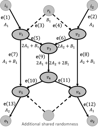
Figure 2: Butterfly network with our code

IV-B Example of networks with $n$-source nodes

The next example is depicted in Fig. 3. The graph $(\tilde{V},\tilde{E})$ is given as follows. The set of nodes $\tilde{V}$ is composed of $v_{1},\ldots,v_{n+2}$, and the set of quantum channels $\tilde{E}$ is composed of $\mathbf{e}(2n+1),\cdots,\mathbf{e}(4n+1)$. The vertex $v_{j}$ is connected to the vertices $v_{n+1}$ and $v_{n+2}$ via the edges $\mathbf{e}(2n+j)$ and $\mathbf{e}(3n+j)$ respectively where $1\leq j\leq n$. And, the vertex $v_{n+1}$ is connected to the vertex $v_{n+2}$ via the edge $\mathbf{e}(4n+1)$. The source nodes are given as $v_{1},\ldots,v_{n}$, and there is single terminal node $v_{n+2}$. Each source node $v_{j}$ ($1\leq j\leq n$) intends to transmit a $q$-dimensional quantum message to the terminal node $v_{n+2}$, where $q$ is a prime power and at the same time it is relatively prime to $n$ and $n-1$. And, all the source nodes $v_{1},\ldots,v_{n}$ share one random number $b_{1}$ of the field $\mathbb{F}_{q}$. Therefore, the $n$ input vertices $i_{1},\cdots,i_{n}$ are connected to source nodes $v_{1},\ldots,v_{n}$ via input edges $\mathbf{e}(1),\cdots,\mathbf{e}(n)$, respectively. One shared-randomness vertex $r_{1}$ is connected to source nodes $v_{1},\ldots,v_{n}$ via shared-randomness edges $\mathbf{e}(n+1),\cdots,\mathbf{e}(2n)$, respectively. The terminal node $v_{n+2}$ is connected to $n$ output vertices $o_{1},\cdots,o_{n}$ via the output edges $\mathbf{e}(4n+2),\cdots,\mathbf{e}(5n+1)$, respectively.

The network code $\{\theta_{j,k}\}_{j\in\{2n+1,\cdots,5n+1\},k\in\mathop{\mathbf{I}}\nolimits(j)}$ is defined as follows:

$$\begin{array}[]{rclrclrcl}\theta_{2n+k,k}&=&n,&\theta_{2n+k,n+k}&=&1,\\ \theta_{3n+k,k}&=&1,&\theta_{3n+k,n+k}&=&1\\ \theta_{4n+1,2n+k}&=&n^{-1},\\ \theta_{4n+k+1,3n+k}&=&1-(n-1)^{-1},&\theta_{4n+k+1,3n+l}&=&-(n-1)^{-1},&\theta_{4n+k+1,4n+1}&=&(n-1)^{-1},\end{array}$$ (70)

where $1\leq k\leq n$, $1\leq l\leq n$ and $k\neq l$.

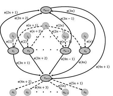
Figure 3: The network of the first example, which consists of $n$ input vertices, one shared-randomness vertex, $n$ output vertices, and $n+2$ nodes

The set of the protected edges $E_{P}$ consists of the $n+1$ edges $\mathbf{e}(3n+1),\cdots,\mathbf{e}(4n+1)$ connecting to the terminal node $v_{n+2}$. Since all the protected edges connected to the unique terminal node $v_{n+2}$, it is not necessary to send the measurement outcomes of the states received from the channel $\mathbf{e}(3n+1),\cdots,\mathbf{e}(4n+1)$. Therefore, we need not consume any additional secret randomness in order to hold back the measurements outcomes.

We can easily construct the $(5n+1)\times(n+1)$ matrix $M_{0}$ made from $\{\theta_{j,k}\}$, i.e.

$$m_{0}(j,k)= \left\{\begin{array}[]{cl}\delta(j,k)&\makebox{if $1\leq j\leq n$ and $1\leq k\leq n+1$}\\ \delta(n,k)&\makebox{if $n<j\leq 2n$ and $1\leq k\leq n+1$}\\ \delta(j-2n,k)n+\delta(n+1,k)&\makebox{if $2n<j\leq 3n$ and $1\leq k\leq n+1$}\\ \delta(j-3n,k)+\delta(n+1,k)&\makebox{if $3n<j\leq 4n$ and $1\leq k\leq n+1$}\\ 1&\makebox{if $j=4n+1$ and $1\leq k\leq n+1$}\\ \delta(j-4n-1,k)&\makebox{if $4n+1<j\leq 5n+1$ and $1\leq k\leq n+1$},\end{array}\right.$$ (77)

and we can check that the condition (5) satisfies; that is, we can successfully send $n$ messages parallelly by the corresponding classical network code. From Theorem 1, that fact guarantees that the corresponding quantum network code given in Protocol 1 transmits the desired quantum states correctly if there is no attack.

Now, we assume that Eve attacks only one of the edges $\mathbf{e}(2n+1),\cdots,\mathbf{e}(4n+1)$, i.e. $E_{A}=\{{\mathbf{e}(j_{0})}\}$ for a certain $j_{0}$ which satisfies $2n+1\leq j_{0}\leq 4n+1$. From Theorem 2, we know that it is enough to check the secrecy and recoverability of the corresponding classical network codes in order to guarantee the security of the transmitted quantum states,

From the definition, the $1\times(n+2)$ matrix $M_{\varsigma}$ is equal to $(m_{0}(j_{0},1),\cdots,m_{0}(j_{0},n+1),0)$. Since the matrix $M_{\varsigma}$ have a single raw and the $n+1$-th column of the matrix is non-zero, we can construct the function $\vec{\mathfrak{b}}$ which satisfies the relation (5), i.e. the corresponding classical network code is secure against Eve’s attack on the edge $\{\mathbf{e}(j_{0})\}$.

The recoverability of the corresponding classical network code is shown as follows. When $E_{A}=\{{\mathbf{e}(3n+k)}\}$ with $1\leq k\leq n$,

$$M_{\iota}\left(\vec{a},0,c_{1}\right)^{T}=(a_{1},\cdots,a_{k-1},c_{1},a_{k+1}\cdots,a_{n},\sum_{i=1}^{n}a_{i}).$$ (78)

When $E_{A}=\{{\mathbf{e}(2n+k)}\}$ with $1\leq k\leq n$,

$$M_{\iota}\left(\vec{a},0,c_{1}\right)^{T}=(a_{1},\cdots,a_{n},\sum_{i=1}^{n}a_{i}-a_{k}+c_{1}).$$ (79)

When $E_{A}=\{{\mathbf{e}(4n+1)}\}$,

$$M_{\iota}\left(\vec{a},0,c_{1}\right)^{T}=(a_{1},\cdots,a_{n},c_{1}).$$ (80)

In every case, it is easy to check that there exists a function $f_{0}$ satisfying (19). The existence is equivalent to meeting the second condition in Lemma 3 which is given in Appendix A holds. Therefore, the classical network code is recoverable for any Eve’s attacks on any single communication channel in $\tilde{E}$.

Therefore, Theorem 2 indicates that the quantum network coding given by Fig. 3 with (70) is secure for any Eve’s attacks on any single quantum channel in $\tilde{E}$.

IV-C Network that is secure against all attacks on any two edges

The network of the next example is shown in Fig. 4. The corresponding graph $(\tilde{V},\tilde{E})$ is formally given as follows. The set of nodes $\tilde{V}$ is composed of $v_{1},\ldots,v_{5}$, and the set of quantum channels $\tilde{E}$ is composed of $\mathbf{e}(7),\cdots,\mathbf{e}(14)$. $v_{1}$ is connected to $v_{3}$, $v_{4}$, and $v_{5}$ via $\mathbf{e}(7)$, $\mathbf{e}(9)$, and $\mathbf{e}(11)$ respectively. $v_{2}$ is also connected to $v_{3}$, $v_{4}$, and $v_{5}$ via $\mathbf{e}(8)$, $\mathbf{e}(10)$, and $\mathbf{e}(12)$. And, $v_{5}$ is additionally connected from $v_{3}$ and $v_{4}$ via $\mathbf{e}(13)$ and $\mathbf{e}(14)$.

The source nodes are given as $v_{1},v_{2}$ and the terminal node is given as $v_{5}$. Source nodes $v_{1}$ and $v_{2}$ intend to transmit a $q$-dimensional quantum message to terminal node $v_{5}$, where we assume that $q$ is relatively prime to $2$, $3$, and $5$. In this network, all source nodes $v_{1},v_{2}$ share two random numbers $b_{1}$ $b_{2}$ of the finite field $\mathbb{F}_{q}$. As a result, the two input vertices $i_{1},i_{2}$ are connected to source nodes $v_{1},v_{2}$ via input edges $\mathbf{e}(1),\mathbf{e}(2)$, respectively. A shared-randomness vertex $r_{1}$ ($r_{2}$) is connected to source nodes $v_{1}$, $v_{2}$ via the shared-randomness edges $\mathbf{e}(3),\mathbf{e}(4)$ ($\mathbf{e}(5),\mathbf{e}(6)$), respectively. The two output vertices $o_{1},o_{2}$ are connected from terminal node $v_{5}$ via output edges $\mathbf{e}(15),\mathbf{e}(16)$, respectively.

Then, the network code is defined by the following parameters:

$$\begin{array}[]{rclrclrclrcl}\theta_{7,1}&=&1,&\theta_{7,3}&=&1,&\theta_{7,5}&=&0,\\ \theta_{9,1}&=&1,&\theta_{9,3}&=&1,&\theta_{9,5}&=&1,\\ \theta_{11,1}&=&1,&\theta_{11,3}&=&0,&\theta_{11,5}&=&1,\\ \theta_{8,2}&=&1,&\theta_{8,4}&=&2,&\theta_{8,6}&=&1,\\ \theta_{10,2}&=&2,&\theta_{10,4}&=&1,&\theta_{10,6}&=&2,\\ \theta_{12,2}&=&1,&\theta_{12,4}&=&1,&\theta_{12,6}&=&3,\\ \theta_{13,7}&=&1,&\theta_{13,8}&=&1,\\ \theta_{14,9}&=&1,&\theta_{14,10}&=&1,\\ \theta_{15,11}&=&3\times 4^{-1},&\theta_{15,12}&=&-2^{-1},&\theta_{15,13}&=&0,&\theta_{15,14}&=&4^{-1},\\ \theta_{16,11}&=&-5\times 8^{-1},&\theta_{16,12}&=&-3\times 4^{-1},&\theta_{16,13}&=&-2^{-1},&\theta_{16,14}&=&9\times 8^{-1},\end{array}$$ (91)

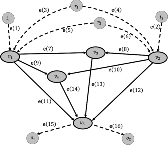
Figure 4: The network of the first example, which consists of $n$ input vertices, one shared-randomness vertices, $n$ output vertices, and $n+2$ nodes

The set of the protected edges $E_{P}$ consists of the four edges $\mathbf{e}(11),\mathbf{e}(12),\mathbf{e}(13),\mathbf{e}(14)$ connecting to terminal node $v_{5}$. Since this network has the single terminal node $v_{5}$, it is not necessary to send all the measurement outcomes from edges $\mathbf{e}(11),\mathbf{e}(12),\mathbf{e}(13),\mathbf{e}(14)$. Thus, we need not consume any additional secret randomness to hold back the measurement outcomes.

By straightforward calculations, we can check that the network code satisfies condition (5); therefore, we can successfully send $2$ characters parallelly with the corresponding classical network code. That is, Theorem 1 guarantees that the corresponding quantum network code given in Protocol 1 transmits the desired quantum messages correctly if there is no attack on all the edges.

Now, we assume that Eve attacks any two of edges in the set $\tilde{E}$; $E_{A}=\{\mathbf{e}(j_{0}),\mathbf{e}(k_{0})\}$ for $7\leq j_{0}<k_{0}\leq 14$. From Theorem 2, we can guarantee the security of the transmitted quantum message by checking the secrecy and recoverability of the corresponding classical network codes.

This network coding satisfies $n^{\prime}=h=2$. We can directly calculate $M_{\varsigma,2}$ and verify that $M_{\varsigma,2}$ is an invertible matrix for any choice of $E_{A}=\{\mathbf{e}(j_{0}),\mathbf{e}(k_{0})\}$ with $7\leq j_{0}<k_{0}\leq 14$. For example, in the case of $j_{0}=8$, and $k_{0}=13$, we can evaluate $M_{\varsigma,2}$ as $\left(\begin{array}[]{cc}2&1\\ 1&0\end{array}\right)$. Thus, Corollary 1 guarantees the secrecy of this classical network code against Eve’s attack.

We next focus on the recoverability of the corresponding classical network code. From the second condition in Lemma 3 proved in the Appendix A, we only need to consider the case where all random variables are fixed to $0$. In this case the information on the edges on $\mathbf{e}(11),\mathbf{e}(12),\mathbf{e}(13)$, and $\mathbf{e}(14)$ can be written as $A_{1}$, $A_{2}$, $A_{1}+A_{2}$, and $A_{1}+2A_{2}$, respectively, where $A_{1}$ and $A_{2}$ are the information sent from $I_{1}$ and $I_{2}$, respectively if there are no disturbances. Hence, we can recover $A_{1}$ and $A_{2}$ from any two of the edges. Now, from the topology of the graph, Eve’s attack on $E_{A}=\{\mathbf{e}(j_{0}),\mathbf{e}(k_{0})\}$ affects at most two of these edges. Therefore, the protected edges $E_{P}$ including the above edges are recoverable.

Finally, from Theorem 2, the quantum network coding given by Fig. 4 with Eq.(91) is secure for all Eve’s attack on the any two of quantum channels in $\tilde{E}$.

IV-D Quantum threshold ramp secret sharing

Quantum secret sharing (QSS) [41] is a protocol to encrypt a quantum state into a multipartite state so that each system (share) has no information and an original state can be reproduced from a collection of the systems. Various different QSS schemes have been developed [41, 42, 43, 44, 45, 46]. Among them, a $(k,L,n)$-threshold ramp QSS scheme is defined as a QSS scheme with $n$ shares having the following property [43]: The original state can be reconstructed from any $k$ shares, and any $k-L$ shares has no information. Hence, partial information of the original state can be drived from $t$ shares with $k>t>k-L$. The network codes given in the above subsections $B$ and $C$ are strongly related to $(k,L,n)$-threshold ramp QSS scheme with $k=n$. Here, the condition $k=n$ means that all the $n$ shares are required to reconstruct the original state.

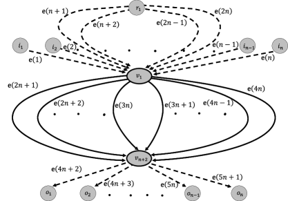
Figure 5: The network that can be derived from the second example by contracting the edge $\mathbf{e}(4n+1)$ and merging vertices $\mathbf{v}_{i}$ with $1\leq i\leq n$ in graph theoretical sense

The network code given in the subsection $B$ is related to a $(2n,2n-1,2n)$-threshold ramp QSS scheme. Let us consider a new network in Fig. 5 which can be derived from the network in Fig. 3 by the following modification of the graph. $n-1$ vertices from $v_{2}$ to $v_{n}$ are also merged into the vertex $v_{1}$, i,e, a set of vertices $\{v_{i}\}_{1\leq i\leq n}$ are replaced by a single vertex $v_{1}$. The vertex $v_{n+1}$ is also merged into the vertex $v_{n+2}$. As a result, the edge $\mathbf{e}(4n+1)$ disappears. All the edges connected to an old replaced vertex are connected to the corresponding new vertex, and all the edges connected from an old replaced vertex are connected from the corresponding new vertex. Following this modification, the network code is also modified as follows:

$$\begin{array}[]{rclrclrcl}\theta_{2n+k,k}&=&n,&\theta_{2n+k,n+k}&=&1,\\ \theta_{3n+k,k}&=&1,&\theta_{3n+k,n+k}&=&1\\ \theta_{4n+k+1,3n+k}&=&1-(n-1)^{-1},&\theta_{4n+k+1,3n+l}&=&-(n-1)^{-1},&\theta_{4n+k+1,2n+l}&=&n^{-1}(n-1)^{-1},\end{array}$$ (95)

where $1\leq k\leq n$, $1\leq l\leq n$ and $k\neq l$. Note that, the indexing of the vertices $v_{j}$ and edges $\mathbf{e}(j)$ breaks the general description rule defined in the previous section in order to make it easy to compare this example and that in the subsection B. From the security analysis of the subsection B, this network code, which does not have any intermediate nodes, is apparently secure against Eve’s attack on any one of the $2n$ channels. On the other hand, all the information on $2n$ channels are required to recover the original quantum state. Further, since the classical randomness is used only in $v_{1}$, the classical randomness can be generated on the node $v_{1}$. Hence, as a protocol sending $n$-quantum messages from the input node $v_{1}$ to the output node $v_{n+2}$, this network coding is nothing but $(2n,2n-1,2n)$ quantum threshold ramp secret sharing scheme [43].

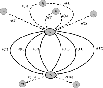
Figure 6: The network that can be derived from the third example by contracting the edge $\mathbf{e}(4n+1)$ and merging vertices $\mathbf{v}_{i}$ with $1\leq i\leq n$ in graph theoretical sense

The network code given in the subsection $C$ is also related to a $(6,4,6)$ quantum ramp secret sharing scheme. Let us consider a new network in Fig. 6 which can be derived from the network in Fig. 4 by the following modification of the graph operations. The vertex $v_{2}$ is merged into the vertex $v_{1}$. The vertices $v_{3}$ and $v_{4}$ are also merged into the vertex $v_{5}$. As a result, the edges $\mathbf{e}(13)$ and $\mathbf{e}(14)$ disappears. All the edges connected to an old replaced vertex are connected to the corresponding new vertex, and all the edges connected from an old replaced vertex are connected from the corresponding new vertex. Following this modification, the network code is also modified as follows:

$$\begin{array}[]{rclrclrclrcl}\theta_{7,1}&=&1,&\theta_{7,3}&=&1,&\theta_{7,5}&=&0,\\ \theta_{9,1}&=&1,&\theta_{9,3}&=&1,&\theta_{9,5}&=&1,\\ \theta_{11,1}&=&1,&\theta_{11,3}&=&0,&\theta_{11,5}&=&1,\\ \theta_{8,2}&=&1,&\theta_{8,4}&=&2,&\theta_{8,6}&=&1,\\ \theta_{10,2}&=&2,&\theta_{10,4}&=&1,&\theta_{10,6}&=&2,\\ \theta_{12,2}&=&1,&\theta_{12,4}&=&1,&\theta_{12,6}&=&3,\\ \theta_{15,9}&=&4^{-1}&\theta_{15,10}&=&4^{-1},&\theta_{15,11}&=&3\times 4^{-1},&\theta_{15,12}&=&-2^{-1},\\ \theta_{16,7}&=&-2^{-1},&\theta_{16,8}&=&-2^{-1},&\theta_{16,9}&=&9\times 8^{-1},&\theta_{16,10}&=&9\times 8^{-1},\\ \theta_{16,11}&=&-5\times 8^{-1},&\theta_{16,12}&=&-3\times 4^{-1},\end{array}$$ (105)

From the security analysis of the subsection C, this new network code, which does not have any intermediate nodes, is apparently secure against Eve’s attack on any two of the $6$ channels. On the other hand, all the information on $6$ channels are required to recover the original quantum state. Further, since the classical randomness is used only in $v_{1}$, the classical randomness can be generated on the node $v_{1}$. Hence, as a protocol sending a quantum message from the input node $v_{1}$ to the output node $v_{5}$, this network coding is nothing but $(6,4,6)$ quantum threshold ramp secret sharing scheme [43].

V Advantages of our quantum network code against quantum error correcting code on partially corrupted quantum network

In this paper, we give a way to make protocols of secure transfer of quantum messages on quantum networks designed originated from classical network coding. However, it has been already investigated to construct such a protocol designed originated from quantum error correcting code, i.e. quantum error correcting code on partially corrupted quantum network [30, 31, 32]. Therefore, we think that it is fair to compare the secure quantum network coding given in this paper and the quantum error correcting code on partially corrupted quantum network.

As a special property of quantum information, it is well known that, if quantum messages can be transferred with fidelity $1$, it is guaranteed that any other party can’t get any information about the quantum messages. Therefore, it is natural to apply this property to construct protocols of secure transfer of quantum messages on quantum network which is made from the following three processes. 1) By using a quantum error correcting code, a quantum message is encoded into several quantum characters at the source nodes. 2) The quantum characters are sent to terminal nodes via a quantum network. 3) At the terminal nodes, the transmitted quantum characters are decoded into the original quantum message. If the amount of disturbances by Eve is bounded by a threshold given by the error correcting code, the secrecy and reliability of the transfer of the message are simultaneously guaranteed. Such an idea has been discussed by several papers [30, 31, 32]. However, our construction of the quantum network coding has two advantages against these previous works.

First advantage is a wide applicability. Even in the previous papers [30, 31, 32], operations in the intermediate nodes are designed originated from classical network coding automatically. However, all the operations on the intermediate node are restricted to be unitary operations. For example, all the node operations are quantum unitary gates designed originated from arbitrary bijective linear maps [31]. As a result, only the bijective functions can be used to design the quantum operators. Strictly speaking, only the invertible functions can be used. From this restriction, we can’t construct a quantum network protocol by simple application of quantum error correcting code even on the butterfly network for example. Therefore, very restricted types of quantum network protocols can be constructed from the previous papers especially in the sense of the variety on the intermediate nodes. In the case of quantum network coding in this paper, the operations in the intermediate nodes are CPTP map generally, i.e. unitary operations and measurement operations. As a result, we can design the node operations originated even from irreversible linear maps. Note that such a property is inherited from the previous result regarding the construction of quantum network coding designed originated from classical network coding without secrecy [10] which is a basis of our result.

Second advantage is an improvement of the secrecy. As we mentioned, in the quantum network protocol made from quantum error correcting code, the secrecy and reliability is indistinguishable. As a result, the secrecy of the code is deeply connected to theoretical limits of quantum error correction. However, in the quantum network coding proposed here, even if the terminal node can’t recover the original quantum message, it is possible that the two conditions in Theorem 2 hold with respect to the set $E_{P}$ of the protected edges. In this case, the secrecy of the quantum message is guaranteed. Therefore, the secrecy is not necessarily restricted by theoretical limits of error correcting code.

VI Conclusion

Based on a secure classical network code, we have proposed a canonical way to make a secure quantum network code in the multiple-unicast setting. This protocol certainly transmits quantum states when there is no attack. While our protocol needs classical communications, they are limited to one-way communications i.e., all of the classical information is given by predefined measurements on nodes and only the final operators on the terminal nodes are affected by the information. Hence, it does not require verification process, which ensures single-shot security. We have also shown the secrecy of the quantum network code under the secrecy and the recoverability of the corresponding classical network code. Our security proof focuses on the classical recoevrbility and the classical secrecy [47].

Our protocol offers secrecy different from that of QKD. While our protocol has the restriction of the number of attacked edges, our protocol does not require repetitive quantum communications because it does not need a verification process. In contrast, QKD needs repeatative quantum communications, which enables us to verify the non-existence of the eavesdropper and to ensure the security. Finally, although the previous result [28] can be applied only to a special secure code on the butterfly network, our secure network code can be applied to any secure classical network code. We have demonstrated several application of our code construction in various network including the butterfly network. These applications show applicability of our method.

Appendix A Lemmas for classical network code

We give a corollary and a lemma for classical network coding that are used for the analysis on our examples given in the section IV.

A-A Corollary for secrecy

We can obtain the following corollary of Lemma 2, which is useful for actual analysis.

Corollary 1.

When $h=n^{\prime}$, a (classical) network code is secure for all of Eve’s attacks on $E_{A}$, if $M_{\varsigma,2}$ is invertible. In particular, when $h=n^{\prime}=1$, the (classical) network code is secure for all Eve’s attack on $E_{A}$, if $M_{\varsigma,2}\neq 0$.

Proof.

When $M_{\varsigma,2}$ is invertible, $M_{\varsigma,2}$ is surjective. Thus, the image of $M_{\varsigma,1}$ is contained in that of $M_{\varsigma,2}$.

When $h=n^{\prime}=1$, $M_{\varsigma,2}$ is just an element of a finite field. Hence, it is invertible if and only if it is non-zero. ∎

A-B Lemma for recoverability

We can relax the recoverability condition from Definition 2 as follows:

Lemma 3.

The following three conditions are equivalent:

1. The messages are recoverable for Eve’s attack on $E_{A}$ by $E_{P}$.

2. There exists a function $f_{\vec{0}_{n^{\prime}}}:\mathbb{F}_{q}^{\left|E_{P}\right|}\rightarrow\mathbb{F}_{q}^{n}$ satisfying

   $$f_{\vec{0}_{n^{\prime}}}\left(M^{\prime}_{\iota}\cdot\left(\vec{a},\vec{0}_{n^{\prime}}\vec{c}\right)^{T}\right)=\vec{a}$$ (106)

   for all $\vec{a}\in\mathbb{F}_{q}^{n}$ and $\vec{c}\in\mathbb{F}_{q}^{h}$.

3. There exist an $n$-by-$\left|E_{P}\right|$ matrix $\mathfrak{M}_{1}$ and an $n$-by-$n^{\prime}$ matrix $\mathfrak{M}_{2}$ such that the relation

   $$\mathfrak{M}_{1}\cdot M^{\prime}_{\iota}\cdot\left(\vec{a},\vec{b},\vec{c}\right)^{T}=\vec{a}+\mathfrak{M}_{2}\cdot\vec{b}$$ (107)

   holds for any vectors $\vec{a}\in\mathbb{F}_{q}^{n}$, $\vec{b}\in\mathbb{F}_{q}^{n^{\prime}}$, and $\vec{c}\in\mathbb{F}_{q}^{h}$.

The last condition in this lemma means that if there exists a decoder, it can be always chosen as a linear decoder.

Proof:

Since the directions 3)$\Rightarrow$1)$\Rightarrow$2) is trivial, we show only 2)$\Rightarrow$3).

Assume 2). We easily find that $f_{\vec{0}_{n^{\prime}}}$ can be restricted to be linear since the condition (106) demands the function $f_{\vec{0}_{n^{\prime}}}$ to be linear on the region expressed by the form $M^{\prime}_{\iota}\cdot(\vec{a},\vec{0}_{n^{\prime}}\vec{c})^{T}$ for any vectors $\vec{a}\in\mathbb{F}_{q}^{n}$, and $\vec{c}\in\mathbb{F}_{q}^{h}$. Hence, $f_{\vec{0}_{n^{\prime}}}$ on the image of $M^{\prime}_{\iota}$ can be written as an $n$-by-$\left|E_{P}\right|$ matrix $\mathfrak{M}_{1}$. Since the map $\vec{b}\mapsto\mathfrak{M}_{1}\cdot M^{\prime}_{\iota}\cdot\left(\vec{0}_{n},\vec{b},\vec{0}_{h}\right)^{T}$ is linear, there exists an $n$-by-$n^{\prime}$ matrix $\mathfrak{M}_{2}$ such that $\mathfrak{M}_{2}\vec{b}=\mathfrak{M}_{1}\cdot M^{\prime}_{\iota}\cdot\left(\vec{0}_{n},\vec{b},\vec{0}_{h}\right)^{T}$. Thus,

$$\mathfrak{M}_{1}\cdot M^{\prime}_{\iota}\cdot\left(\vec{a},\vec{b},\vec{c}\right)^{T}= \mathfrak{M}_{1}\cdot M^{\prime}_{\iota}\cdot\left(\vec{a},\vec{0}_{n^{\prime}},\vec{c}\right)^{T}+\mathfrak{M}_{1}\cdot M^{\prime}_{\iota}\cdot\left(\vec{0}_{n},\vec{b},\vec{0}_{h}\right)^{T}$$

$$= \vec{a}+\mathfrak{M}_{2}\vec{b},$$

which implies 3). ∎

Appendix B Constructions of matrices describing network

In this appendix, we concretely construct the matrices describing the network structure.

B-A Construction of $M_{0}$

The definition of input edges and shared-randomness edges determine the coefficients $\left\{m_{0}\left(j,k\right)\right\}_{j,k}$ for $1\leq j\leq n+l$ as follows: For $1\leq j\leq n$, $\mathbf{e}\left(j\right)$ is an input edge, that is, $\mathbf{e}\left(j\right)\in E_{I}$. Thus, the definition of input edges determines $\left\{m_{0}\left(j,k\right)\right\}_{k=1}^{n+n^{\prime}}$ as

$$\left\{m_{0}\left(j,k\right)\right\}_{k=1}^{n+n^{\prime}}=(\vec{0}_{j-1},1,\vec{0}_{n+n^{\prime}-j})\quad\mbox{for }1\leq j\leq n.$$ (108)

For $n+1\leq j\leq n+l$, $\mathbf{e}\left(j\right)$ is a shared-randomness edge, that is, $\mathbf{e}\left(j\right)\in E_{R}$. Hence, there uniquely exists an integer $j^{\prime}\in[1,n^{\prime}]$ such that $n+\sum_{k^{\prime}=1}^{j^{\prime}-1}l_{k^{\prime}}<j\leq n+\sum_{k^{\prime}=1}^{j^{\prime}}l_{k^{\prime}}$. Thus, the definition of shared-randomness edges determines $\left\{m_{0}\left(j,k\right)\right\}_{k=1}^{n+n^{\prime}}$ as

$$\left\{m_{0}\left(j,k\right)\right\}_{k=1}^{n+n^{\prime}} =(\vec{0}_{n+i^{\prime}-1},1,\vec{0}_{n^{\prime}-i^{\prime}})\quad\mbox{for }n<j\leq n+l.$$ (109)

By substituting the expression (4) of $Y_{j}$ into the relation (3), we derive the recurrence relation of $m_{0}\left(j,k\right)$ as

$$m_{0}\left(j,k\right)=\sum_{k^{\prime}<j}\theta_{j,k^{\prime}}m_{0}\left(k^{\prime},k\right)\quad\mbox{for }n+l<j\leq N+2n+l.$$ (110)

Note that $M_{0}$ is a matrix which identifies the relation between the character transferred on the edges and the combination of messages and shared-secure-random number in the case that there is no disturbance for every channel. Therefore, we can use Eq.(3) and (4).

The Eqs. (108),(109), and (110) enable us to evaluate all the coefficients of the $(N+2n+l)\times(n+n^{\prime})$ matrix $M_{0}$, i.e. $\left\{m_{0}\left(j,k\right)\right\}_{j,k}$, recursively.

B-B Construction of $M$

In the case of $1\leq j\leq n+l$, $Y_{j}$ is not affected by disturbances by definition. Therefore,

$$m\left(j,k\right) = \left\{\begin{array}[]{cl}m_{0}\left(j,k\right)&\makebox{for $1\leq j\leq n+l$ and $1\leq k\leq n+n^{\prime}$}\\ 0&\makebox{for $1\leq j\leq n+l$ and $n+n^{\prime}<k\leq n+n^{\prime}+h$}\end{array}\right.$$ (113)

$M$ is a matrix which identifies the relation between the character transferred on the edges and the combination of messages, shared-secure-random number and injected character. That means, we consider the case that there may exist disturbances. Therefore, we have to use the relation

$$Y_{j}=\sum_{k<j}\theta_{j,k}Y_{k}^{\prime}\quad\mbox{for }n+l<j\leq N+2n+l$$

instead of the the relation Eq.(3). By substituting the expressions (6) and (10) of $Y_{j}$ and $Y_{j}^{\prime}$ into the above relation, we obtain the relation

$$m\left(j,k\right)=\sum_{k^{\prime}<j}\theta_{j,k^{\prime}}m^{\prime}(k^{\prime},k)\quad\mbox{for }n+l<j\leq N+2n+l.$$ (114)

By combining (13) for the above relation, we derive the following recurrence relations for $m\left(j,k\right)$:

$$m\left(j,k\right)=\sum_{k^{\prime}<j}\theta_{j,k^{\prime}}m\left(k^{\prime},k\right)+\sum_{k^{\prime}=1}^{h}\theta_{j,\varsigma\left(k^{\prime}\right)}(\delta_{k,n+n^{\prime}+k^{\prime}}-m\left(\varsigma\left(k^{\prime}\right),k\right))\Theta(j-\varsigma\left(k^{\prime}\right)-1),$$ (115)

for $n+l<j\leq N+2n+l$, where $\Theta(y)$ is a step function such that $\Theta(y)=0$ ($\Theta(y)=1$) if $y<0$ ($y\geq 1$).

The Eqs. (113) and (115) enable us to evaluate all the coefficients of the $(N+2n+l)\times(n+n^{\prime}+h)$ matrix $M$ recursively.

References

- [1] A. Kawachi, and T. Koshiba, “Progress in quantum computational cryptography,” Journal of Universal Computer Science, vol. 12, no. 6, pp. 691-709, 2006.
- [2] A. Broadbent, J. Fitzsimons, and E. Kashefi, “Universal blind quantum computation,” Proceedings of the 50th Annual IEEE Symposium on Foundations of Computer Science, pp. 517-526, 2009.
- [3] T. Morimae, K. Fujii, “Blind quantum computation protocol in which Alice only makes measurements,” Physical Review A, vol. 87, no. 5, 050301(R), May 2013.
- [4] S. Wiesner, “Conjugate Coding,” SIGACT News, vol. 15, no. 1, pp. 78-88, 1983.
- [5] M. Hayashi, K. Iwama, H. Nishimura, R. Raymond, and S. Yamashita, “Quantum Network Coding,” in STACS 2007 SE - 52 (W. Thomas and P. Weil, eds.), vol. 4393 of Lecture Notes in Computer Science, pp. 610-621, Springer Berlin Heidelberg, 2007.
- [6] M. Hayashi, “Prior entanglement between senders enables perfect quantum network coding with modification,” Phys. Rev. A, vol. 76, no. 4, 40301, 2007.
- [7] H. Lu, Z. Li, X. Yin, R. Zhang, X. Fang, L. Li, N. Liu, F. Xu, Y. Chen, and J. Pan, “Experimental quantum network coding,” npj Quantum Inf, vol. 5, 89, 2019.
- [8] H. Kobayashi, F. Le Gall, H. Nishimura, and M. Rötteler, “General Scheme for Perfect Quantum Network Coding with Free Classical Communication,” in Automata, Languages and Programming SE - 52 (S. Albers, A. Marchetti-Spaccamela, Y. Matias, S. Nikoletseas, and W. Thomas, eds.), vol. 5555 of Lecture Notes in Computer Science, pp. 622-633, Springer Berlin Heidelberg, 2009.
- [9] D. Leung, J. Oppenheim, and A. Winter, “Quantum Network Communication; The Butterfly and Beyond,” IEEE Transactions on Information Theory, vol. 56, no. 7, pp. 3478-3490, 2010.
- [10] H. Kobayashi, F. Le Gall, H. Nishimura, and M. Rotteler, “Perfect quantum network communication protocol based on classical network coding,” in Proceedings of 2010 IEEE International Symposium on Information Theory (ISIT), pp. 2686-2690, 2010.
- [11] H. Kobayashi, F. Le Gall, H. Nishimura, and M. Rotteler, “Constructing quantum network coding schemes from classical nonlinear protocols,” in Proceedings of 2011 IEEE International Symposium on Information Theory (ISIT), pp. 109-113, 2011.
- [12] A. Jain, M. Franceschetti, and D. A. Meyer, “On quantum network coding,” Journal of Mathematical Physics vol. 52, 032201 (2011)
- [13] R. Ahlswede, N. Cai, S. -Y. R. Li, and R. W. Yeung, “Network information flow,” IEEE Transactions on Information Theory, vol. 46, no. 4, pp. 1204-1216, 2000.
- [14] N. Cai and R. Yeung, “Secure network coding,” in Proceedings of 2002 IEEE International Symposium on Information Theory (ISIT), pp. 323-, 2002.
- [15] N. Cai and R. W. Yeung, “Network error correction, Part 2: Lower bounds,” Commun. Inf. and Syst., vol. 6, no. 1, pp. 37-54, Jan. 2006.
- [16] K. Bhattad, S. Member, and K. R. Narayanan, “Weakly Secure Network Coding,” in First Workshop on Network Coding, Theory, and Applications, (Riva del Garda), 2005.
- [17] R. L. R. Liu, Y. L. Y. Liang, H. Poor, and P. Spasojevic, “Secure Nested Codes for Type II Wiretap Channels,” 2007 IEEE Information Theory Workshop, pp. 337-342, 2007.
- [18] S. Y. E. Rouayheb and E. Soljanin, “On Wiretap Networks II,” in Proceedings of 2007 IEEE International Symposium on Information Theory (ISIT), pp. 551-555, 2007.
- [19] K. Harada and H. Yamamoto, “Strongly Secure Linear Network Coding,” IEICE transactions on Fundamentals of Electronics, Communications and Computer Sciences, vol. E91-A, no. 10, pp. 2720-2728, 2008.
- [20] T. H. T. Ho, B. L. B. Leong, R. Koetter, M. Medard, M. Effros, and D. Karger, “Byzantine Modification Detection in Multicast Networks With Random Network Coding,” IEEE Transactions on Information Theory, vol. 54, no. 6, pp. 2798-2803, 2008.
- [21] S. Jaggi, M. Langberg, S. Katti, T. Ho, D. Katabi, M. Medard, and M. Effros, “Resilient Network Coding in the Presence of Byzantine Adversaries,” IEEE Transactions on Information Theory, vol. 54, no. 6, pp. 2596-2603, 2008.
- [22] L. Nutman and M. Langberg, “Adversarial models and resilient schemes for network coding,” in Proceedings of 2008 IEEE International Symposium on Information Theory (ISIT), pp. 171-175, 2008.
- [23] Z. Y. Z. Yu, Y. W. Y. Wei, B. Ramkumar, and Y. G. Y. Guan, “An Efficient Signature-Based Scheme for Securing Network Coding Against Pollution Attacks,” IEEE INFOCOM 2008 - The 27th Conference on Computer Communications, 2008.
- [24] N. Cai and T. Chan, “Theory of Secure Network Coding,” Proceedings of the IEEE, vol. 99, pp. 421-437, 2011.
- [25] N. Cai and R. W. Yeung, “Secure Network Coding on a Wiretap Network,” IEEE Transactions on Information Theory, vol. 57, no. 1, pp. 424-435, 2011.
- [26] R. Matsumoto and M. Hayashi, “Secure Multiplex Network Coding,” 2011 International Symposium on Networking Coding (2011): DOI: 10.1109/ISNETCOD.2011.5979076.
- [27] R. Matsumoto and M. Hayashi, “Universal Secure Multiplex Network Coding with Dependent and Non-Uniform Messages,” IEEE Transactions on Information Theory, vol. 63, no. 6, pp. 3773-3782, 2017.
- [28] M. Owari, G. Kato, and M. Hayashi, “Secure Quantum Network Coding on Butterfly Network,” Quantum and Technology, vol. 3, 014001, 2017.
- [29] G. Kato, M. Owari, and M. Hayashi, “Single-Shot Secure Quantum Network Coding for General Multiple Unicast Network with Free Public Communication,” In: Shikata J. (eds) 10th International Conference on Information Theoretic Security (ICITS2017). Lecture Notes in Computer Science, vol. 10681. Springer, pp. 166-187.
- [30] S. Song and M. Hayashi, “Quantum Network Code for Multiple-Unicast Network with Quantum Invertible Linear Operations,” In: S. Jeffery (eds) 13th Conference on the Theory of Quantum Computation, Communication and Cryptography (TQC 2018). Leibniz International Proceedings in Informatics (LIPIcs), vol. 111. pp. 10:1–10:20. Centre for Quantum Software and Information (QSI), University of Technology Sydney, July 16 – 18, 2018.
- [31] S. Song and M. Hayashi, “Secure Quantum Network Code without Classical Communication,” IEEE Trans. Inform. Theory, vol. 66, no. 2, pp. 1178-1192, 2020.
- [32] M. Hayashi and S. Song, “Quantum Capacity of Partially Corrupted Quantum Network,” arXiv:1911.02860 (2019).
- [33] F. Cheng and V. Y. F. Tan, “A Numerical Study on the Wiretap Network With a Simple Network Topology,” IEEE Transactions on Information Theory, vol. 62, no. 5, pp. 2481-2492, (2016)
- [34] G. Kato, M. Owari, and M. Murao, “Multicast quantum network coding” Japan patent JP2014-192875A (in Japanese)
- [35] G. Kato, M. Owari, and M. Murao “Multicast quantum netowk coding” Japan patent JP2015-220621A (in Japanese)
- [36] Y. Hirota and M. Owari “Asymmetric quantum multicast network coding: asymmetric optimal cloning over quantum networks” arXiv:1908.00705 (2019)
- [37] G. K. Agarwal, M. Cardone, and C. Fragouli, “On (Secure) Information flow for Multiple-Unicast Sessions: Analysis with Butterfly Network,” arXiv: 1606.07561 (2016).
- [38] C. H. Bennett, G. Brassard, C. Crépeau, R. Jozsa, A. Peres, and W. K. Wootters, “Teleporting an unknown quantum state via dual classical and einstein-podolsky-rosen channels,” Phys. Rev. Lett., vol. 70, pp. 1895-1899, 1993.
- [39] M. Hayashi, M. Owari, G. Kato, and N. Cai, “Secrecy and Robustness for Active Attack in Secure Network Coding and its Application to Network Quantum Key Distribution,” arXiv: 1703.00723 (2017); “Secrecy and Robustness for Active Attack in Secure Network Coding,” IEEE International Symposium on Information Theory (ISIT2017), Aachen, Germany, 25-30 June 2017. pp. 1172-1177
- [40] M. Hayashi, Group Representation for Quantum Theory, Springer (2017)
- [41] R. Cleve, D. Gottesman, and H.-K. Lo, “How to share a quantum secret” Physical Review Letters, vol.83, pp. 648-, 1999.
- [42] D. Gottesman, “Theory of quantum secret sharing”, Physical Review A, vol.61, 042311, 2000.
- [43] T. Ogawa, A. Sasaki, M. Iwamoto, and H. Yamamoto, “Quantum secret sharing schemes and reversibility of quantum operations”, Physical Review A, vol.72, 032318, 2005.
- [44] F.-G. Deng, X.-H. Li, C.-Y. Li, P. Zhou, and H.-Y. Zhou “Multiparty quantum-state sharing of an arbitrary two-particle state with Einstein-Podolsky-Rosen pairs,” Physical Review A, vol.72, 044301, 2005.
- [45] D. Markham and B. C. Sanders, “Graph states for quantum secret sharing”, Phys. Rev. A vol.78, 042309, 2008.
- [46] Y.G. Yang, Y.W. Teng, H.P. Chai, Q.Y. Wen, “Verifiable quantum -threshold secret key sharing.” International Journal of Theoretical Physics vol. 50, no. 3, pp. 792-798, 2011.
- [47] J. M. Renes, “Duality of privacy amplification against quantum adversaries and data compression with quantum side information,” Proc. Roy. Soc. A, vol.467, no. 2130, pp. 1604-1623, 2011.