Long Alternating Paths Exist

Abstract

Let $P$ be a set of $2n$ points in convex position, such that $n$ points are colored red and $n$ points are colored blue. A non-crossing alternating path on $P$ of length $\ell$ is a sequence $p_{1},\dots,p_{\ell}$ of $\ell$ points from $P$ so that (i) all points are pairwise distinct; (ii) any two consecutive points $p_{i},p_{i+1}$ have different colors; and (iii) any two segments $p_{i}p_{i+1}$ and $p_{j}p_{j+1}$ have disjoint relative interiors, for $i\neq j$.

We show that there is an absolute constant $\varepsilon>0$, independent of $n$ and of the coloring, such that $P$ always admits a non-crossing alternating path of length at least $(1+\varepsilon)n$. The result is obtained through a slightly stronger statement: there always exists a non-crossing bichromatic separated matching on at least $(1+\varepsilon)n$ points of $P$. This is a properly colored matching whose segments are pairwise disjoint and intersected by common line. For both versions, this is the first improvement of the easily obtained lower bound of $n$ by an additive term linear in $n$. The best known published upper bounds are asymptotically of order $4n/3+o(n)$.

1 Introduction

We study a family of problems that were discovered independently in two different (but essentially equivalent) settings. Researchers in discrete and computational geometry found a geometric formulation, while researchers in computational biology and stringology studied circular words. Around 1989, Erdős asked the following geometric question [4, p. 409]: given a set $P$ of $n$ red and $n$ blue points in convex position, how many points of $P$ can always be collected by a non-intersecting polygonal path $\pi$ with vertices in $P$ such that the vertex-color along $\pi$ alternates between red and blue. Taking every other segment of $\pi$, we obtain a properly colored set of pairwise disjoint segments with endpoints in $P$. A closely related problem asks for a large separated matching, a collection of such segments with the extra property that all of them are intersected by a common line. This is equivalent to finding a long antipalindromic subsequence in a circular sequence of $2n$ bits, where $n$ bits are $0$ and $n$ bits are $1$, see Figure 1. This formulation was stated in 1999 in a paper on protein folding [9]. Similar questions were also studied for palindromic subsequences [13]. One such question is equivalent to finding many disjoint monochromatic segments with endpoints in $P$, a problem that was also studied by the geometry community.

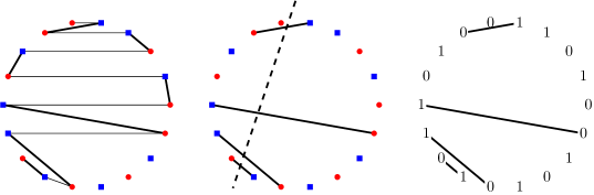
Figure 1: Left: a set $P$ of $18$ points in convex position, $9$ of them red and $9$ of them blue, with an alternating path of length $15$ (this is not a longest such path). Taking every other segment, we obtain a properly colored disjoint matching on $P$. Middle: a separated matching on $P$, with a dashed line that intersects all matching edges (this is not a maximum such matching). Right: an antipalindromic subsequence on a circular word of $18$ bits, $9$ of them $0$ and $9$ of them $1$.

An easy lower bound for alternating paths is $n$, and the best known lower bound is $n+\Omega(\sqrt{n})$ [10]. We increase this to $cn+o(n)$, for a constant $c>1$. Similarly, for the other mentioned problems, we improve the lower bounds by an additive term of $\varepsilon n$, for some fixed $\varepsilon>0$. Also here, this constitutes the first $\Omega(n)$ improvement over the trivial lower bounds.

1.1 The (geometric) setting

We have a set $P$ of $2n$ points $p_{0},p_{1},\dots,p_{2n-1}$ in convex position, numbered in clockwise order. The points in $P$ are colored red and blue, so that there are exactly $n$ red points and $n$ blue points. The goal is to find a long non-crossing alternating path in $P$. That is, a sequence $\pi:q_{0},q_{1},\dots,q_{\ell-1}$ of points in $P$ such that (i) each point from $P$ appears at most once in $\pi$; (ii) $\pi$ is alternating, i.e., for $i=0,\dots,\ell-2$, we have that $q_{i}$ is red and $q_{i+1}$ is blue or that $q_{i}$ is blue and $q_{i+1}$ is red; (iii) $\pi$ is non-crossing, i.e., for $i,j\in\{0,\dots,\ell-2\}$, $i\neq j$, the two segments $q_{i}q_{i+1}$ and $q_{j}q_{j+1}$ intersect only in their endpoints and only if they are consecutive in $\pi$, see Figure 1(left). We will also just say alternating path for $\pi$. Alternating paths for planar point sets in general (not just convex) position have been studied in various previous papers, e.g., [1, 2, 3, 5, 6].

For most of this work, we will focus on another, closely related, structure. A non-crossing separated bichromatic matching $M$ in $P$ is a set $\{p_{1}q_{1},p_{2}q_{2},\dots,p_{k}q_{k}\}$ of $k$ pairs of points in $P$, such that (i) all points $p_{1},\dots,p_{k},q_{1},\dots,q_{k}$ are pairwise distinct; (ii) the segments $p_{i}q_{i}$ and $p_{j}q_{j}$ are disjoint, for all $1\leq i<j\leq k$; (iii) for $i=1,\dots,k$, the points $p_{i}$ and $q_{i}$ have different colors; and (iv) there exists a line that intersects all segments $p_{1}q_{1},p_{2}q_{2},\dots,p_{k}q_{k}$, see Figure 1(middle). Often, we will just use the term separated bichromatic matching or simply separated matching for $M$.

1.2 Previous results

The following basic lemma says that a large separated matching immediately yields a long alternating path. The (very simple) proof was given by Kynčl, Pach, and Tóth [8, Section 3].

Lemma 1.1.

Suppose that a bichromatic convex point set $P$ admits a separated matching with $k$ segments. Then, $P$ has an alternating path of length $2k$.

Let $l(n)$ be the largest number such that for every set $P$ of $n$ red and $n$ blue points in convex position, there is an alternating path of length at least $l(n)$. Around 1989, Erdős and others [8] conjectured that $\lim_{n\rightarrow\infty}l(n)/n=3/2$. Abellanas, García, Hurtado, and Tejel [1] and, independently, Kynčl, Pach, and Tóth [8, Section 3] disproved this by showing the upper bound $l(n)\leq 4n/3+O(\sqrt{n})$. Kynčl, Pach, and Tóth [8] also improved the (almost trivial) lower bound $l(n)\geq n$ to $l(n)\geq n+\Omega(\sqrt{n/\log n})$. They conjectured that in fact $l(n)=4n/3+o(n)$. In her PhD thesis [10] (see also [7, 12, 11]), Mészáros improved the lower bound to $l(n)\geq n+\Omega(\sqrt{n})$, and she described a wide class of configurations where every separated matching has at most $2n/3+O(\sqrt{n})$ edges. This also implies the upper bound $l(n)\leq 4n/3+O(\sqrt{n})$ mentioned above [1, 8]. It was announced to us in personal communication that E. Csóka, Z. Blázsik, Z. Király, and D. Lenger constructed configurations with an upper bound of $cn+o(n)$ on the size of the largest separated matching, where $c=2-\sqrt{2}\approx 0.5858$.

1.3 Our results

We improve the almost trivial lower bound $n/2$ for separated matchings to $n/2+\varepsilon n$.

Theorem 1.2.

There is a fixed $\varepsilon>0$ such that any convex point set $P$ with $n$ red and $n$ blue points admits a separated matching with at least $n/2+\varepsilon n$ edges.

By Lemma 1.1, we obtain the following corollary about long alternating paths.

Theorem 1.3.

There is a fixed $\varepsilon>0$ such that any convex point set $P$ with $n$ red and $n$ blue points admits an alternating path with at least $n+\varepsilon n$ vertices.

A variant of Theorem 1.2 also holds for the monochromatic case. The definition of a non-crossing separated monochromatic matching, or simply separated monochromatic matching, is obtained from the definition of a separated bichromatic matching by changing condition (iii) to (iii’) for $i=1,\dots,k$, the points $p_{i}$ and $q_{i}$ have the same color. Some of the upper bound constructions for separated bichromatic matchings apply to the monochromatic setting, also giving the upper bound $2n/3+O(\sqrt{n})$. Here is a monochromatic version of Theorem 1.2.

Theorem 1.4.

There are constants $\varepsilon>0$ and $n_{0}\in\mathbb{N}$ such any convex point set $P$ with $n\geq n_{0}$ points, colored red and blue, admits a separated monochromatic matching with at least $n/2+\varepsilon n$ vertices.

There are two differences between the statement of Theorem 1.2 and Theorem 1.4: we do not require that the number of red and blue points in $P$ is equal (and hence the size of the matching is stated in terms of vertices instead of edges), and we need a lower bound on the size of $P$. This is necessary, because Theorem 1.4 does not always hold for, e.g., $n=4$. It was announced to us in a personal communication that the construction of E. Csóka, Z. Blázsik, Z. Király and D. Lenger from above also gives the upper bound $cn+o(n)$ on the size of a largest separated monochromatic matching, where $c=2-\sqrt{2}\approx 0.5858$.

1.4 Our results in the setting of finite words

As we already said, the problems in this paper were independently discovered by researchers in computational biology and stringology. In a study on protein folding algorithms, Lyngsø and Pedersen [9] formulated a conjecture that is equivalent to saying that the bound in Theorem 1.2 can be improved to $2n/3$ (for $n$ divisible by $3$). Müllner and Ryzhikov [13, p. 461] write that this conjecture “has drawn substantial attention from the combinatorics of words community”. For the convenience of readers from this community, we rephrase our theorems for separated matchings in the finite words setting. We use the terminology of Müllner and Ryzhikov [13], without introducing it here. The following corresponds to Theorem 1.2.

Theorem 1.5.

There is a fixed $\varepsilon>0$ such that for any even $n\in\mathbb{N}$, every binary circular word of length $n$ with equal number of zeros and ones has an antipalindromic subsequence of length at least $n/2+\varepsilon n$.

The following corresponds to Theorem 1.4.

Theorem 1.6.

There are constants $\varepsilon>0$ and $n_{0}\in\mathbb{N}$ so that for any $n\in\mathbb{N}$, $n\geq n_{0}$, every binary circular word of length $n$ has a palindromic subsequence of length at least $n/2+\varepsilon n$.

2 Existence of large separated bichromatic matchings

In this section, we prove our main result: large separated bichromatic matchings exist.

2.1 Runs and separated matchings

A run of $P$ is a maximal sequence $p_{i},p_{i+1},\dots,p_{i+\ell}$ of consecutive points with the same color. That is, for $j=i,\dots,i+\ell-1$, the color of $p_{j}$ and of $p_{j+1}$ are the same, and the colors of $p_{i-1}$ and $p_{i}$ and the colors of $p_{i+\ell}$ and $p_{i+\ell+1}$ are different. The number of runs is always even. Kynčl, Pach, and Tóth showed that if $P$ contains $t$ runs, then $P$ admits an alternating path of length $n+\Omega(t)$ [8, Lemma 3.2]. We will need the following analogous result for separated matchings.

Theorem 2.1.

Let $c_{1}=1/32$ and $t\geq 4$. Let $P$ be a bichromatic convex point set with $2n$ points, $n$ red and $n$ blue, and suppose that $P$ has $t$ runs. Then, $P$ admits a separated matching with at least $n/2+c_{1}t^{2}/n$ edges.

Proof 2.2.

We partition the edges of the complete geometric graph on $P$ into $2n$ parallel matchings $M_{0},\dots,M_{2n-1}$, see Figure 2.

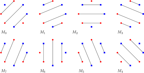
Figure 2: We partition the edges of the complete geometric graph on $P$ into $2n$ parallel matchings.

For $i=0,\dots,2n-1$, let $M_{i}^{\prime}$ be the submatching of $M_{i}$ that consists of the bichromatic edges of $M_{i}$. Every $M_{i}^{\prime}$ is a separated matching, and the $2n$ matchings $M_{0}^{\prime},\dots,M_{2n-1}^{\prime}$ together contain all the $n^{2}$ bichromatic edges on $P$. Thus, the average number of edges in a matching from $M_{0}^{\prime},\dots,M_{2n-1}^{\prime}$ is $n^{2}/2n=n/2$.

Suppose now that $p_{j}$ and $p_{k}$ are two distinct red points such that $p_{j}$ is the (clockwise) first point of a red run and $p_{k}$ is the (clockwise) last point of a different red run. Let $M_{i}$ be the parallel matching that contains the edge $p_{j}p_{k}$. Then, $p_{j-1}$ and $p_{k+1}$ are blue, and either $p_{j-1}=p_{k+1}$ or $p_{j-1}p_{k+1}$ is a monochromatic blue edge in $M_{i}$. Thus, the matching that is obtained from $M_{i}^{\prime}$ by adding the bichromatic edge $p_{j}p_{k+1}$ is still a separated matching, and similarly for the matching $M_{i}^{\prime\prime}$ obtained from $M_{i}^{\prime}$ by making all the possible additions of this kind, see Figure 3.

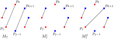
Figure 3: For any monochromotic edge $p_{j}p_{k}$ in $M_{j}$ that connects the first (clockwise) point $p_{j}$ of a red run with the last (clockwise) point $p_{k}$ of another red run, we add to $M_{j}^{\prime}$ the bichromatic edge $p_{j}p_{k+1}$. The resulting matching is called $M_{i}^{\prime\prime}$.

Since there are $t/2$ red runs, the total number of edges that we add in the matchings $M_{0}^{\prime\prime},\dots,M_{2n-1}^{\prime\prime}$ is $\binom{t/2}{2}$. Hence, the average size of a matching from $M_{0}^{\prime\prime},\dots,M_{2n-1}^{\prime\prime}$ is

$$\frac{n}{2}+\frac{\binom{t/2}{2}}{2n}=\frac{n}{2}+\frac{t(t-2)}{16n}\geq\frac{n}{2}+\frac{t^{2}}{32n},$$

since $t\geq 4$ and hence $t-2\geq t/2$. In particular, at least one of the matchings $M_{i}^{\prime\prime}$ has the desired number of edges.

2.2 Chunks, partitions, and configurations

Let $k\in\{1,\dots,n\}$. A $k$-chunk is a sequence of consecutive points in $P$ with exactly $k$ points of one color and less than $k$ points of the other color. Hence, a $k$-chunk has at least $k$ and at most $2k-1$ points. A clockwise $k$-chunk with starting point $p_{i}$ is the shortest $k$-chunk that starts from $p_{i}$ in clockwise order. A counterclockwise $k$-chunk with starting point $p_{i}$ is defined analogously, going in the counterclockwise direction. For a $k$-chunk $C$, we denote by $r(C)$ the number of red points and by $b(C)$ the number of blue points in $C$. We call $C$ a red chunk if $r(C)=k$ (and hence $b(C)<k$) and a blue chunk if $b(C)=k$ (and hence $r(C)<k$). The index of $C$ is $b(C)/k$ for a red chunk and $r(C)/k$ for a blue chunk. Thus, the index of $C$ lies between $0$ and $(k-1)/k$, and it measures how “mixed” $C$ is.

Next, let $k\in\{1,\dots,n\}$ and $\lambda\in\mathbb{N}\cup\{0\}$. We define a $(k,\lambda)$-partition. Suppose that $k$ is odd. First, we construct a maximum sequence $C_{0},C_{1},\dots$ of clockwise disjoint $k$-chunks, as follows: we begin with the clockwise $k$-chunk $C_{0}$ with starting point $p_{0}$, and we let $\ell_{0}$ be the number of points in $C_{0}$. Next, we take the clockwise $k$-chunk $C_{1}$ with starting point $p_{\ell_{0}}$, and let $\ell_{1}$ be the number of points in $C_{1}$. After that, we take the clockwise $k$-chunk $C_{2}$ with starting point $p_{\ell_{0}+\ell_{1}}$, and so on. We stop once we reach the last $k$-chunk that does not overlap with $C_{0}$. Next, we construct a maximum sequence $D_{0},D_{1},\dots$ of counterclockwise $(k+3)$-chunks, starting with the point $p_{2n-1}$, in an analogous manner. Let $\lambda^{\prime}$ be the minimum of $\lambda$ and the number of $(k+3)$-chunks $D_{i}$. Now, to obtain the $(k,\lambda)$-partition, we take $\lambda^{\prime}$ counterclockwise $(k+3)$-chunks $D_{0},\dots,D_{\lambda^{\prime}-1}$ and a maximum number of clockwise $k$-chunks $C_{0},C_{1},\dots$ that do not overlap with $D_{0},\dots,D_{\lambda^{\prime}-1}$. If $k$ is even, the $(k,\lambda)$-partition is defined analogously, switching the roles of the clockwise and the counterclockwise direction.

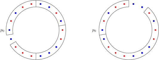
Figure 4: A set of 18 points and its $(3,0)$-partition (left) and $(3,1)$-partition (right). In the $(3,0)$-partition, the first chunk is red with index $2/3$, the second chunk is blue with index $1/3$, the third chunk is blue with index $2/3$, and the fourth chunk is red with index $0$. The average red index is $1/3$, the average blue index is $1/2$. The index of the $(3,0)$-partition is $1/2$. The $(3,1)$-partition has one clockwise $3$-chunk and one counterclockwise $6$-chunk. The $3$-chunk is red with index $2/3$, the $6$-chunk is red with index $5/6$. The average red index is $3/4$, the average blue index is $0$ The index of the $(3,1)$-partition is $3/4$.

There may be some points that do not lie in any chunk of the $(k,\lambda)$-partition. We call these points uncovered.

The average red index of $\Gamma$ is the average index in a red chunk of $\Gamma$ ($0$, if there are no red chunks). The average blue index of $\Gamma$ is defined analogously. The index of $\Gamma$ is the maximum of the average red index and the average blue index of $\Gamma$. The max-index color is the color whose average index achieves the index of $\Gamma$, the other color is called the min-index color, see Figure 4 for an illustration of the concepts so far. The following simple proposition helps us bound the number of chunks.

Proposition 2.3.

Let $P$ be a convex bichromatic point set with $2n$ points, $n$ red and $n$ blue, and let $\Gamma$ be a $(k,\lambda)$-partition of $P$. In $\Gamma$, there are at most $2k-2$ uncovered points, at most $k-1$ of them red and at most $k-1$ of them blue. Furthermore, let $R$ be the number of red chunks and $B$ the number of blue chunks in $\Gamma$, and let $\alpha$ be the index of $\Gamma$. Then,

$$R+B\leq\frac{2n}{k}\quad\text{and}\quad\max\{R,B\}\leq\frac{n}{k}.$$ (1)

Furthermore, we have

$$R+B\geq\left\lfloor\frac{2n}{2k+5}\right\rfloor>\frac{2n}{7k}-1,\quad\max\{R,B\}\geq\frac{1}{2}\left\lfloor\frac{2n}{2k+5}\right\rfloor>\frac{n}{7k}-\frac{1}{2},\\ \text{and}\quad\min\{R,B\}\geq\frac{1-\alpha}{2}\left\lfloor\frac{2n}{2k+5}\right\rfloor-\frac{k-1}{k+3}>(1-\alpha)\frac{n}{7k}-2.$$ (2)

If $\lambda=0$, the lower bounds improve to

$$R+B\geq\left\lfloor\frac{2n}{2k-1}\right\rfloor\geq\frac{n}{k}-1,\quad\max\{R,B\}\geq\frac{1}{2}\left\lfloor\frac{2n}{2k-1}\right\rfloor>\frac{n}{2k}-\frac{1}{2},\\ \text{and}\quad\min\{R,B\}\geq\frac{1-\alpha}{2}\left\lfloor\frac{2n}{2k-1}\right\rfloor-\frac{k-1}{k}>(1-\alpha)\frac{n}{2k}-2.$$ (3)

Proof 2.4.

Since a red chunk in $\Gamma$ contains at least $k$ red points, we have $R\leq n/k$. Similarly, $B\leq n/k$, and (1) follows.

Any chunk in $\Gamma$ has at most $2k+5$ points. Thus, the total number of chunks is at least $R+B\geq\lfloor 2n/(2k+5)\rfloor>2n/7k-1$, using $k\geq 1$. This is the first bound of (2). The second bound follows from the inequality $\max\{R,B\}\geq(R+B)/2$. For the third bound, suppose that $R=\max\{R,B\}$ and $B=\min\{R,B\}$. Let $\gamma$ be the difference between the number of uncovered blue points and the number of uncovered red points in $\Gamma$. Since the number of red points in $P$ is the same as the number of blue points, we have

$$0=\gamma+\sum_{C}(b(C)-r(C))+\sum_{D}(b(D)-r(D)),$$ (4)

where the first sum ranges over the red chunks $C$ of $\Gamma$, and the second sum ranges over the blue chunks $D$ of $\Gamma$. Now, we have $\gamma\leq k-1$, since there are at most $k-1$ uncovered blue points. Furthermore, we have

$$\sum_{C}(b(C)-r(C))=\sum_{C}r(C)\left(\frac{b(C)}{r(C)}-1\right)\leq(k+3)\sum_{C}\left(\frac{b(C)}{r(C)}-1\right)=(k+3)(\alpha-1)R,$$

since $r(C)\leq k+3$ for every chunk $C$ and $(1/R)\sum_{C}b(C)/r(C)=\alpha$. Finally, we have $b(D)-r(D)\leq k+3$ for every blue chunk $D$. Thus, (4) implies that

$$0\leq k-1+(k+3)(\alpha-1)R+(k+3)B\quad\Rightarrow\quad B\geq(1-\alpha)R-\frac{k-1}{k+3}.$$

Using the previous lower bound on $R$, this gives

$$B\geq\frac{1-\alpha}{2}\left\lfloor\frac{2n}{2k+5}\right\rfloor-\frac{k-1}{k+3}>(1-\alpha)\frac{n}{7k}-2,$$

and hence (2). To obtain (3), we argue in the same manner, but we use the fact that for $\lambda=0$, all chunks have at most $2k-1$ points and exactly $k$ points of the majority color.

The purpose of the $(k,\lambda)$-partitions is to transition smoothly between the $(k,0)$-partition and the $(k+3,0)$-partition. In our proof, this will enable us to gradually increase the chunk-sizes, while keeping the index under control.

A $k$-configuration of $P$ is a partition of $P$ into $k$-chunks, leaving no uncovered points, see Figure 5. In contrast to a $(k,\lambda)$-partition, the chunks in a $k$-configuration are not necessarily minimal. Note that while $P$ always has a $(k,\lambda)$-partition, it does not necessarily admit a $k$-configuration. The average red index, the average blue index, etc. of a $k$-configuration are defined as for a $(k,\lambda)$-partition. The following proposition helps us bound the number of chunks in a $k$-configuration.

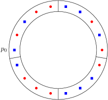
Figure 5: A set of 18 points and a $3$-configuration for it. The chunk from $p_{0}$ is red with index $2/3$, the next clockwise chunk is blue with index $2/3$, followed by another blue chunk of index $1/3$ and a final red chunk of index $1/3$. The average blue index and the average red index are both $1/2$. Note that the chunks are not minimal.

Proposition 2.5.

Let $P$ be a convex bichromatic point set with $2n$ points, $n$ red and $n$ blue, and let $\Gamma$ be a $k$-configuration of $P$. Let $R$ be the number of red chunks, $B$ the number of blue chunks,$\alpha$ the average red index and $\beta$ the average blue index of $\Gamma$. Then,

$$n=kR+\beta kB=kB+\alpha kR.$$ (5)

Furthermore, $R+B\geq n/k$, $\max\{R,B\}\geq n/2k$, and $\min\{R,B\}\geq(1-\max\{\alpha,\beta\})n/2k$. Finally, $\max\{R,B\}=R$ if and only if $\alpha\geq\beta$.

Proof 2.6.

The red chunks in $\Gamma$ contain $kR$ red points and $\alpha kR$ blue points, while the blue chunks contain $kB$ blue points and $\beta kB$ red points. All points are covered by the chunks, and there are $n$ red points and $n$ blue points. This implies (5). Since all points in $P$ are covered by the chunks in $\Gamma$, the lower bound $R+B\geq\lfloor 2n/(2k-1)\rfloor$ from (3) becomes $R+B\geq 2n/(2k-1)\geq n/k$, and hence also $\max\{R,B\}\geq n/2k$. Finally, from (5), we get $(1-\alpha)R=(1-\beta)B$, so $\max\{R,B\}=R$ if and only if $\alpha\geq\beta$, i.e., the number of chunks of the max-index color is at least the number of chunks of the min-index color. This also implies that $B\geq(1-\alpha)R$ and $R\geq(1-\beta)B$. In particular, $\min\{R,B\}\geq(1-\max\{\alpha,\beta))\max\{R,B\}$.

In our proof, the key challenge will be to analyze $k$-configurations with small constant index (say, around $0.1$).

2.3 From $(k,\lambda)$-partitions to $k$-configurations

Our first goal is to show that we can focus on $(k,\lambda)$-partitions with large $k$ and constant, but not too large index. We begin by noting that if the $(k,0)$-partition of $P$ for a constant $k$ has a large index, then we can find a long alternating path in $P$.

Lemma 2.7.

Set $c_{2}=1/12800$. Let $k,n\in\mathbb{N}$ with $8k^{2}\leq n$. Let $P$ be a convex bichromatic point set with $2n$ points, $n$ red and $n$ blue. If the $(k,0)$-partition $\Gamma$ of $P$ has index at least $0.1$, then $P$ admits a separated matching of size at least $(1/2+c_{2}/k^{4})n$.

Proof 2.8.

If $P$ has only two runs, then $P$ has a separated matching of size $n$, and the theorem follows since $n/2\geq c_{2}(n/k^{4})$. Thus, assume that $P$ has at least $4$ runs, and suppose for concreteness that the max-index color in $\Gamma$ is red. Let $R$ be the number of red chunks in $\Gamma$. Since the index of $\Gamma$ is at most $(k-1)/k$, by (3), we have

$$R\geq\frac{1}{k}\cdot\frac{n}{2k}-2=\frac{n-4k^{2}}{2k^{2}}\geq\frac{n-n/2}{k^{2}}=\frac{n}{2k^{2}},$$

since $n\geq 8k^{2}$ and hence $4k^{2}\leq n/2$. The average red index is at least $0.1$, and the index of a chunk is at most $1$. Thus, there must be at least $0.1R\geq 0.05(n/k^{2})$ red chunks with positive index and hence at least $0.05(n/k^{2})$ chunks with at least one red point and one blue point. In particular, $P$ has at least $0.05(n/k^{2})$ runs. We also assumed that $P$ has at least four runs. Thus, by Theorem 2.1, it follows that $P$ admits a separated matching of size

$$\frac{n}{2}+\frac{n^{2}}{400k^{4}\cdot 32n}=\left(\frac{1}{2}+\frac{c_{2}}{k^{4}}\right)n.$$

Next, we show that if the $(k,0)$-partition still has a small index for $k=\Omega(n)$, then we can find a large separated matching.

Lemma 2.9.

Set $c_{3}=1/81$. Let $k,n\in\mathbb{N}$ with $k\leq n$ and $6480n\leq k^{2}$. Let $P$ be a convex bichromatic point set with $2n$ points. If the $(k,0)$-partition $\Gamma$ of $P$ has index at most $0.1$, then $P$ admits a separated matching of size at least $(1/2+c_{3}(k/n)^{2})n$.

Proof 2.10.

We adapt an argument by Kynčl, Pach, and Tóth [8, Lemma 3.1]. Set $i_{0}=\lceil\log(2n/k)\rceil$. Then

$$k\in\left[\left\lceil\frac{2n}{2^{i_{0}}}\right\rceil,\left\lceil\frac{2n}{2^{{i_{0}}}}\cdot 2\right\rceil\right).$$

Since the index of $\Gamma$ is at most $0.1$, there is a $k$-chunk $C^{\prime}$ in $\Gamma$ with index at most $0.1$. For concreteness, assume that $C^{\prime}$ is red. We truncate $C^{\prime}$ to the first $\lceil 2n/2^{i_{0}}\rceil$ elements in clockwise direction, calling the resulting interval $C$. Since $C^{\prime}$ has index at most $0.1$, it follows that $C$ contains at most

$$0.1\cdot k<0.1\cdot\left\lceil\frac{2n}{2^{i_{0}}}\cdot 2\right\rceil\leq 0.1\cdot 2\cdot\left\lceil\frac{2n}{2^{i_{0}}}\right\rceil=0.2|C|$$

blue points and hence at least $0.8|C|$ red points. We now define a sequence $D_{0},D_{1},\dots,D_{i_{0}-1}$ of pairwise disjoint intervals. The intervals are consecutive in clockwise order after $C$: first come the points from $C$, then the points from $D_{0}$, then from $D_{1}$, etc. The number of points in $D_{i}$ is chosen to be

$$|D_{i}|=\left\lceil\frac{2n}{2^{i_{0}}}\cdot{2^{i+1}}\right\rceil-\left\lceil\frac{2n}{2^{i_{0}}}\cdot{2^{i}}\right\rceil.$$

Furthermore, for $i=0,\dots,i_{0}-1$, we set $F_{i}=C\cup\bigcup_{j=0}^{i}D_{j}$. By construction, we have

$$|F_{i}|=\left\lceil\frac{2n}{2^{i_{0}}}\cdot 2^{i+1}\right\rceil,$$

for $i=0,\dots,i_{0}-1$. In particular, $F_{i_{0}-1}=P$, see Figure 6. Note that the size of $F_{i}$ and the size of $D_{i+1}$ differ by at most $1$, where always $|F_{i}|\geq|D_{i+1}|$.

Figure 6: The partition of the convex point set into intervals. The size of the intervals roughly doubles in each step. The size of $F_{i}$ is roughly the same as the size of the following $D_{i+1}$.

Now, set $\delta=k/n$ and let $i^{*}$ be the smallest $0\leq i\leq i_{0}-1$ such that $D_{i}$ contains at least

$$\left(\frac{1}{2}+\frac{\delta}{20}\right)|D_{i}|$$

blue points, and set $i^{*}=i_{0}$, if no such $i$ exists. Suppose that $i^{*}\geq 1$. Then, for $j=0\dots,i^{*}-1$, the interval $D_{j}$ contains at least

$$\left(\frac{1}{2}-\frac{\delta}{20}\right)|D_{j}|$$

red points, and hence the total number of red points in the interval $F_{i^{*}-1}$ is at least

$$\phantom{=}\frac{4}{5}|C|+\left(\frac{1}{2}-\frac{\delta}{20}\right)\sum_{j=0}^{i^{*}-1}|D_{j}|$$

$$=\frac{4}{5}\left\lceil\frac{2n}{2^{i_{0}}}\right\rceil+\left(\frac{1}{2}-\frac{\delta}{20}\right)\sum_{j=0}^{i^{*}-1}\left(\left\lceil\frac{2n}{2^{i_{0}}}\cdot{2^{j+1}}\right\rceil-\left\lceil\frac{2n}{2^{i_{0}}}\cdot{2^{j}}\right\rceil\right).$$

The sum telescopes, so this is

$$=\frac{4}{5}\left\lceil\frac{2n}{2^{i_{0}}}\right\rceil+\left(\frac{1}{2}-\frac{\delta}{20}\right)\left(\left\lceil\frac{2n}{2^{i_{0}}}\cdot{2^{i^{*}}}\right\rceil-\left\lceil\frac{2n}{2^{i_{0}}}\right\rceil\right)$$

$$\geq\frac{1}{2}\left\lceil\frac{2n}{2^{i_{0}}}\cdot 2^{i^{*}}\right\rceil+\frac{3}{10}\left\lceil\frac{2n}{2^{i_{0}}}\right\rceil-\frac{\delta}{20}\left\lceil\frac{2n}{2^{i_{0}}}\cdot 2^{i^{*}}\right\rceil.$$

Since for $$a>0 b\in\mathbb{N} b\lceil a\rceil\geq\lceil ba\rceil \lceil a\rceil\geq(1/b)\lceil ab\rceil$$ and , we have , and hence , this is

$$\geq\frac{1}{2}\left\lceil\frac{2n}{2^{i_{0}}}\cdot 2^{i^{*}}\right\rceil+\frac{3}{10}\cdot\frac{1}{2^{i^{*}}}\cdot\left\lceil\frac{2n}{2^{i_{0}}}\cdot{2^{i^{*}}}\right\rceil-\frac{\delta}{20}\left\lceil\frac{2n}{2^{i_{0}}}\cdot 2^{i^{*}}\right\rceil.$$

Using that $$i^{*}\leq i_{0}=\lceil\log(2n/k)\rceil<\log(2n/k)+1=-\log\delta+2 2^{-i^{*}}>2^{\log\delta-2}=\delta/4$$ and thus , we lower bound this as

$$\geq\left(\frac{1}{2}+\frac{3}{10}\cdot\frac{\delta}{4}-\frac{\delta}{20}\right)\left\lceil\frac{2n}{2^{i_{0}}}\cdot 2^{i^{*}}\right\rceil$$

$$=\left(\frac{1}{2}+\frac{\delta}{40}\right)|F_{i^{*}-1}|.$$

It follows that $i^{*}\leq i_{0}-1$, since $F_{i_{0}-1}=P$, and $P$ contains only $n=(1/2)|F_{i_{0}-1}|$ red points.

Now, if $i^{*}=0$, we set $J_{1}=C$ and $J_{2}=D_{0}$. If $i^{*}\geq 1$, we set $J_{1}=F_{i^{*}-1}$ and $J_{2}=D_{i^{*}}$. In this way, we obtain two adjacent intervals $J_{1}$ and $J_{2}$ ($J_{2}$ clockwise from $J_{1}$) such that the following holds: if we write $\ell_{1}=|J_{1}|$ and $\ell_{2}=|J_{2}|$, then (i) $\ell_{1}\geq|C|>k/2$ and $\ell_{2}\geq\ell_{1}-1$; and (ii) $J_{1}$ contains at least $(1/2+\delta/40)\ell_{2}$ red points and $J_{2}$ contains at least $(1/2+\delta/40)\ell_{2}$ blue points. We match the first $(1/2+\delta/40)\ell_{2}$ red points in $J_{1}$, counterclockwise from the common boundary of $J_{1}$ and $J_{2}$, to the first $(1/2+\delta/40)\ell_{2}$ blue points in $J_{2}$, clockwise from the common boundary of $J_{1}$ and $J_{2}$. Let $K\subseteq J_{1}\cup J_{2}$ be the smallest interval that contains the matched edges, and let $L$ be the complementary interval of $P$.

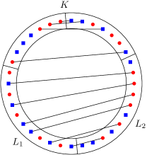
Figure 7: We match the red points in $J_{1}$ to the blue points in $J_{2}$ and find a large separated matching between the remaining points.

The interval $K$ contains exactly $(1/2+\delta/40)\ell_{2}$ red points from $J_{1}$ and at most $(1/2-\delta/40)\ell_{2}$ red points from $J_{2}$. Thus, the number of red points in $K$ is at most $\ell_{2}$. Similarly, the interval $K$ contains exactly $(1/2+\delta/40)\ell_{2}$ blue points from $J_{2}$ and at most $\ell_{1}-(1/2+\delta/40)\ell_{2}\leq 1+(1/2-\delta/40)\ell_{2}$ blue points from $J_{1}$, so the number of blue points in $K$ is at most $\ell_{2}+1$. Setting $m=n-\ell_{2}-1$, it follows that $L$ contains at least $m$ red points and at least $m$ blue points, in particular, $|L|\geq 2m$.

We partition $L$ into two intervals $L_{1}$ and $L_{2}$, each of size at least $m$. Clearly, $L_{1}$ contains at least $m/2$ red points or $m/2$ blue points (or both), and similarly for $L_{2}$. Suppose that $L_{1}$ contains at least $m/2$ red points. If $L_{1}$ has less than $m/2$ blue points, then $L_{2}$ must have at least $m/2$ blue points. If $L_{1}$ has at least $m/2$ blue points, then $L_{1}$ has at least $m/2$ red points and at least $m/2$ blue points, and $L_{2}$ has at least $m/2$ red points or $m/2$ blue points. In any case, it must be that $L_{1}$ contains at least $m/2$ red points and $L_{2}$ contains at least $m/2$ blue points, or vice versa. Thus, we can obtain a bichromatic matching between $L_{1}$ and $L_{2}$ of size at least $m/2$, see Figure 7. Overall, we get a separated matching of size at least

$$\left(\frac{1}{2}+\frac{\delta}{40}\right)\ell_{2}+\frac{1}{2}\left(n-\ell_{2}-1\right) =\frac{n}{2}+\frac{\delta}{40}\cdot\ell_{2}-\frac{1}{2}$$

$$\geq\frac{n}{2}+\frac{\delta k}{80}-\frac{\delta}{40}-\frac{1}{2}$$

$$\geq\frac{n}{2}+\frac{\delta k}{80}-1$$

$$\geq\frac{n}{2}+\frac{\delta^{2}n}{81},$$

since $\ell_{2}\geq\ell_{1}-1\geq k/2-1$ and since

$$\frac{\delta k}{80}-1=\frac{\delta^{2}n-80}{80}\geq\frac{\delta^{2}n-(1/81)\delta^{2}n}{80}=\frac{\delta_{1}^{2}n}{81},$$

as $6480n\leq k^{2}$, so $80\leq k^{2}/(81n)=\delta^{2}n/81$.

Our goal now is to show that we can focus on $k$-configurations with $k$ neither too small nor too large, and of index approximately $0.1$. Here, we only sketch the argument, and we will make it more precise below, once all the lemmas have been stated formally: we choose $k_{1}=O(1)$ and $k_{2}=\Omega(n)$ to satisfy the previous two lemmas, and we consider the sequence of the $(k_{1},0)$-partition, the $(k_{1},1)$-partition, the $(k_{1},2)$-partition, $\ldots$, up to the $(k_{2},0)$-partition of $P$. By Lemma 2.7 and Lemma 2.9, we can assume that the first partition in the sequence has index less than $0.1$ and the last partition in the sequence has index larger than $0.1$. Thus, at some point the index has to jump over $0.1$. Our definition of $(k,\lambda)$-partition ensures that this jump is gradual.

Lemma 2.11.

Let $k,n\in\mathbb{N}$ with $n\geq 210000k$. Let $P$ be a convex bichromatic point set with $2n$ points, $n$ red and $n$ blue. Let $\Gamma_{1}$ be the $(k,\lambda)$-partition and $\Gamma_{2}$ the $(k,\lambda+1)$-partition of $P$. Suppose that the index of $\Gamma_{1}$ is at most $0.1$. Then, the average red index and the average blue index of $\Gamma_{1}$ and $\Gamma_{2}$ each differ by at most $0.001$.

Proof 2.12.

We bound the change of the average red index, the argument for the average blue index is analogous. Let $R$ be the number of red chunks in $\Gamma_{1}$, $R^{\prime}$ the number of red chunks in $\Gamma_{2}$, and let $\alpha(C)$ denote the index of a red chunk $C$ in $\Gamma_{1}$ or $\Gamma_{2}$. We would like to estimate the change of the average red index of from $\Gamma_{1}$ to $\Gamma_{2}$, i.e.,

$$\left|\frac{1}{R^{\prime}}\sum_{C^{\prime}}\alpha(C^{\prime})-\frac{1}{R}\sum_{C}\alpha(C)\right|,$$ (6)

where the first sum goes over all red chunks $C^{\prime}$ in $\Gamma_{2}$ and the second sum goes over all red chunks $C$ in $\Gamma_{1}$. We have

$$(\ref{equ:indexchange}) =\frac{\left|R\sum_{C^{\prime}}\alpha(C^{\prime})-R^{\prime}\sum_{C}\alpha(C)\right|}{R\cdot R^{\prime}}$$

$$\leq\frac{|R-R^{\prime}|}{R\cdot R^{\prime}}\sum_{C_{1}}\alpha(C_{1})+\frac{R}{R\cdot R^{\prime}}\sum_{C_{2}}\alpha(C_{2})+\frac{R^{\prime}}{R\cdot R^{\prime}}\sum_{C_{3}}\alpha(C_{3}),$$

where the first sum goes over all red chunks $C_{1}$ that appear in both $\Gamma_{1}$ and $\Gamma_{2}$, the second sum goes over all red chunks $C_{2}$ that appear only in $\Gamma_{2}$, and the third sum goes over all red chunks $C_{3}$ that appear only in $\Gamma_{1}$. When going from $\Gamma_{1}$ to $\Gamma_{2}$, we add one $(k+3)$-chunk and remove the $k$-chunks that overlap with it. A $(k+3)$-chunk has at most $2k+5$ points, and a $k$-chunk has at least $k\geq 1$ points. Thus, the new $(k+3)$- chunk can overlap at most seven $k$-chunks. This implies that $|R-R^{\prime}|\leq 6$. All indices are in $[0,1)$. Thus, we have $(1/R^{\prime})\sum_{C_{1}}\alpha(C_{1})\leq(1/R^{\prime})\sum_{C^{\prime}}\alpha(C^{\prime})\leq 1$. Moreover, since $\Gamma_{2}$ contains at most one new red chunk, we have $\sum_{C_{2}}\alpha(C_{2})\leq 1$, and since $\Gamma_{1}$ contains at most $7$ red chunks that do not appear in $\Gamma_{2}$, we have $\sum_{C_{3}}\alpha(C_{3})\leq 7$. Thus,

$$(\ref{equ:indexchange})\leq\frac{6}{R}+\frac{1}{R^{\prime}}+\frac{7}{R}.$$

By (2), we have

$$R\geq\frac{(1-0.1)n}{7k}-2=\frac{9n-140k}{70k}\geq\frac{7n}{70k}=\frac{n}{10k},$$

as $n\geq 210000k\geq 70k$. In particular, $R\geq n/(10k)\geq 8$, so $R^{\prime}\geq R-7\geq R/8$. Thus,

$$(\ref{equ:indexchange})\leq\frac{6}{R}+\frac{8}{R}+\frac{7}{R}=\frac{21}{R}\leq\frac{210k}{n}\leq 0.001.$$

It follows that we can assume that we are dealing with a $(k,\lambda)$-partition of index approximately $0.1$. Actually, we will see that it suffices to consider $k$-configurations of index $0.1$. This will be the focus of the next section.

2.4 Random chunk-matchings in $k$-configurations

In this section, we will focus on convex bichromatic point sets $P$ that admit a $k$-configuration $\Gamma$ with special properties. Later, we will see how to reduce to this case.

Let $C_{0},C_{1},\dots,C_{\ell-1}$ be the chunks of the $k$-configuration $\Gamma$. We define a notion of chunk-matching, as illustrated in Figures 8 and 9.

Figure 8: The six chunk matchings $M_{0},\dots,M_{5}$ for a set of six chunks. If $i$ is even, the chunks $C_{i/2}$ and $C_{i/2+3}$ are matched to themselves. If $i$ is odd, every chunk is matched to a different chunk.

Figure 9: The five chunk matchings $M_{0},M_{1},\dots,M_{4}$ for a set of five chunks. In matching $M_{i}$, the chunk $C_{(3i\bmod 5)}$ is matched to itself. Every other chunk is matched to a different chunk.

A chunk matching pairs each of the $\ell$ chunks with another chunk (possibly itself). Our goal is to define chunk matchings in such a way that we can easily derive from a chunk matching a separated matching between the points in $P$.

Formally, we define $\ell$ matchings $M_{0},\dots,M_{\ell-1}$ by saying that for $i,j=0,\dots,\ell-1$, the matching $M_{i}$ pairs the chunks $C_{j}$ and $C_{(i-j)\bmod\ell}$. Again, refer to Figures 8 and 9 for examples. The matching rule is symmetric, i.e., if $C_{a}$ is matched to $C_{b}$ then $C_{b}$ is matched to $C_{a}$. Note that if $j\equiv(i-j)\pmod{\ell}$, the chunk $C_{j}$ is matched to itself in $M_{i}$. If $\ell$ is even, this happens only for even $i$, namely for $j=i/2$ and for $j=i/2+\ell/2$. If $\ell$ is odd, this happens in every matching, namely for $j\equiv(\ell+1)i/2\pmod{\ell}$. By construction, for every $M_{i}$, if we connect the matched chunks by straight line edges, we obtain a set of plane segments such that there is one line that intersects all segments. Furthermore, every pair $C_{i},C_{j}$ of chunks, $0\leq i\leq j\leq\ell-1$ appears in exactly one chunk matching. In essence, these matchings correspond to partitioning the chunks of $\Gamma$ with a line, where the line can possibly pass through one or two chunks of $\Gamma$ that are then matched to themselves.

Next, we describe how to derive from a given chunk matching $M$ a separated matching on $P$, see Figure 10 for an illustration. We look at every two chunks $C$ and $D$ paired my $M$ (possibly, $C$ = $D$). If $C$ is red and $D$ blue, we match the $k$ red points in $C$ to the $k$ blue points in $D$, getting $k$ matched edges. The case that $C$ is blue and $D$ is red is analogous. If $C\neq D$ and both $C$ and $D$ are red, we could match the $k$ red points in $C$ to the $b(D)<k$ blue points in $D$, or vice versa. We choose the option that gives more edges, yielding $\max\{b(C),b(D)\}$ matched edges. The case that $C\neq D$ and both are blue is similar. Finally, suppose that $C=D$, and for concreteness, suppose that $C$ is red. In this case, we split the points in $C$ into two parts, containing $\lceil k/2\rceil$ red points each (if $k$ is odd, the median point belongs to both parts). In one part, we have at least $\lceil b(C)/2\rceil$ blue points, and we match these blue points to the red points in the other part. This yields $\lceil b(C)/2\rceil\geq b(C)/2$ matched edges. Thus, a chunk matching $M$ gives a separated matching with at least

$$\frac{1}{2}\Bigg{(}\sum_{\begin{subarray}{c}(C,D)\in M\\ C\text{ red},D\text{ red}\end{subarray}}\max\{b(C),b(D)\}+\sum_{\begin{subarray}{c}(C,D)\in M\\ C\text{ red},D\text{ blue}\end{subarray}}k\\ +\sum_{\begin{subarray}{c}(C,D)\in M\\ C\text{ blue},D\text{ red}\end{subarray}}k+\sum_{\begin{subarray}{c}(C,D)\in M\\ C\text{ blue},D\text{ blue}\end{subarray}}\max\{r(C),r(D)\}\Bigg{)}$$ (7)

matched edges, where the sums go over all ordered pairs of matched chunks in $M$, i.e., a matched pair $(C,D)$ with $C\neq D$ appears twice (which is compensated by the leading factor of $1/2$) and a matched pair $(C,C)$ appears once. The next lemma shows that a chunk matching that is chosen uniformly at random usually matches half the points of $P$.

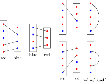
Figure 10: Going from a matched pair of chunks to a separated matching. If the two chunks have different colors, we can match $k$ edges. If the two colors are the same, there are two reasonable options, matching the red points in one chunk with the blue points in the other chunk. We choose the one that matches more edges. A special case occurs if a chunk is matched to itself. In this case, we split the majority color into half and match between the halves.

Lemma 2.13.

Let $\Gamma$ be a $k$-configuration of $P$ and $M$ a random chunk matching in $\Gamma$. The expected number of matched edges in the corresponding separated matching is at least $n/2$.

Proof 2.14.

Let $R$ be the number of red chunks in $\Gamma$ and $B$ the number of blue chunks in $\Gamma$. Let $\alpha$ be the average index of the red chunks, and $\beta$ the average index of the blue chunks. We sum (7) over all $R+B$ possible chunk matchings and take the average. This gives the expected number of matched edges (the sums range over all ordered pairs of chunks in $\Gamma$).

$$\phantom{=}\frac{1}{2(R+B)}\Bigg{(}\sum_{C\text{ red},D\text{ red}}\max\{b(C),b(D)\}+2\sum_{C\text{ red},D\text{ blue}}k$$

$$\qquad+\sum_{C\text{ blue},D\text{ blue}}\max\{r(C),r(D)\}\Bigg{)}$$

Since there are $$R B$$ red chunks and blue chunks, this is

$$=\frac{1}{2(R+B)}\left(\sum_{C\text{ red},D\text{ red}}\max\{b(C),b(D)\}+2kRB+\sum_{C\text{ blue},D\text{ blue}}\max\{r(C),r(D)\}\right)$$

We lower bound the maximum by the average to estimate this as

$$\geq\frac{1}{2(R+B)}\left(\sum_{C\text{ red},D\text{ red}}\frac{b(C)+b(D)}{2}+2kRB+\sum_{C\text{ blue},D\text{ blue}}\frac{r(C)+r(D)}{2}\right)$$ (**)

Simplifying the sums, this is

$$=\frac{1}{2(R+B)}\left(R\sum_{C\text{ red}}b(C)+2kRB+B\sum_{C\text{ blue}}r(C)\right)$$

Since the total number of blue points in red chunks is $$\alpha kR \beta kB$$ and the total number of red points in blue chunks is , this equals

$$=\frac{\alpha kR^{2}+2kRB+\beta kB^{2}}{2(R+B)}$$

Regrouping the terms and using (5), this becomes

$$=\frac{R(\alpha kR+kB)+B(\beta kB+kR)}{2(R+B)}=\frac{(R+B)n}{2(R+B)}=\frac{n}{2}.$$

2.5 Taking advantage of $k$-configurations

One inefficiency in the calculation in Lemma 2.13 is that we bound the maximum by the average in inequality (**). If these two quantities often differ significantly, we can gain an advantage over Lemma 2.13. This is made precise in the next lemma.

Lemma 2.15.

Set $c_{4}=1/40$. Let $\delta>0$ and let $P$ be a convex bichromatic point set with $2n$ points, $n$ red and $n$ blue, and $\Gamma$ a $k$-configuration for $P$ with index at most $0.11$ that contains at least $\delta(n/k)$ red chunks or at least $\delta(n/k)$ blue chunks with index at least $0.22$. Then, $P$ admits a separated matching of size at least $(1/2+c_{4}\delta^{2})n$.

Proof 2.16.

Suppose without loss of generality that there are at least $\delta(n/k)$ red chunks with index at least $0.2$. Let $R$ be the number of red chunks and $B$ the number of blue chunks. The average red index of $\Gamma$ is at most $0.11$. Thus, if writing $\gamma_{1}(n/k)$ for the number of red chunks with index in $(0.11,0.22)$ and $\gamma_{2}(n/k)\geq\delta(n/k)$ for the number of red chunks with index in $[0.22,1)$, we have

$$0.11R\geq 0.11\gamma_{1}\frac{n}{k}+0.22\gamma_{2}\frac{n}{k}=0.11(\gamma_{1}+2\gamma_{2})\frac{n}{k}.$$

It follows that $R\geq(\gamma_{1}+2\gamma_{2})(n/k)$, and there must be at least $\gamma_{2}(n/k)\geq\delta(n/k)$ red chunks of index in $[0,0.11]$. Now, consider the following sum over all ordered pairs $(C,D)$ of red chunks, where one chunk ($C$ or $D$) has red index at most $0.11$ and the other chunk ($D$ or $C$) has red index at least $0.22$:

$$\frac{1}{2(R+B)}\left(\sum_{C}\sum_{D}\max\{b(C),b(D)\}-\frac{b(C)+b(D)}{2}\right)$$

Since $$2\max\{a,b\}-a-b=\max\{a,b\}-\min\{a,b\} a,b\in\mathbb{R}$$, for all , this equals

$$=\frac{1}{4(R+B)}\sum_{C}\sum_{D}(\max\{b(C),b(D)\}-\min\{b(C),b(D)\})$$

One chunk in each summand contains at least $$0.22k 0.11k$$ blue points, the other chunk contains at most blue points, so we can lower bound this as

$$\geq\frac{1}{4(R+B)}\sum_{C}\sum_{D}(0.22-0.11)k$$

$$\geq\frac{1}{4(R+B)}\sum_{C}\sum_{D}\frac{k}{10}\geq\frac{\delta^{2}(n/k)^{2}}{R+B}\frac{k}{20}\geq\frac{\delta^{2}}{40}n,$$

since we are adding over at least $2\delta^{2}(n/k)^{2}$ ordered pairs $(C,D)$ (recall that each ordered pair $(C,D)$ has a partner $(D,C)$ in the sum) and since by (1), we have $R+B\leq 2n/k$. Thus, comparing with (**), the lemma follows.

Lemma 2.15 shows that we can assume that few chunks in the $k$-configuration $\Gamma$ of $P$ have index larger than $0.22$. In fact, suppose now that $\Gamma$ contains no chunk of index at least $0.3$ (this will be justified below). From now on, we will also assume that $k$ is divisible by $3$. We subdivide each chunk in our $k$-configuration $\Gamma$ into three $(k/3)$-subchunks. Since all $k$-chunks have index less than $0.3$, the subchunks have the same color as the original chunk. Let $C$ be a $k$-chunk. The middle subchunk of $C$, denoted by $C_{M}$, is the $(k/3)$-subchunk of $C$ that lies in the middle of the three subchunks. Now, we consider the middle subchunks. If the middle subchunks of the max-index color contain many points of the min-index color, we can gain an advantage by considering two cross-matchings between chunks of the max-index color.

Lemma 2.17.

Set $c_{5}=1/4$. Let $\delta>0$ and let $P$ be a convex bichromatic point set with $2n$ points, $n$ red and $n$ blue. Let $\Gamma$ be a $k$-configuration for $P$ such that (i) $k$ is divisible by $3$; (ii) every chunk in $\Gamma$ has index less than $0.3$; and (iii) the middle subchunks of the max-index color contain in total at least $\delta n$ points of the min-index color. Then $P$ admits a separated matching of size at least $(1/2+c_{5}\delta)n$.

Proof 2.18.

Suppose that the max-index color is red. We take a random chunk matching $M$ of $\Gamma$, and we derive a separated matching from $M$ as described above. However, when considering a pair $(C,D)$ of two red chunks, we proceed slightly differently. First, suppose that $C\neq D$, and let $C_{1},C_{2},C_{3}$ be the three subchunks of $C$, and $D_{1},D_{2},D_{3}$ be the three subchunks of $D$ (in clockwise order). We have $r(C_{i})=r(D_{i})=k/3$, for $i=1,2,3$; and $b(C_{1})+b(C_{2})+b(C_{3})<k/3$ and $b(D_{1})+b(D_{2})+b(D_{3})<k/3$.

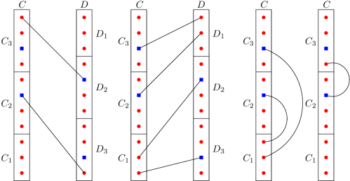
Figure 11: The two different separated matchings between two distinct red chunks (left) and the same red chunk (right).

We consider two separated matchings between $C$ and $D$ (see Figure 11(left): (a) match all blue points in $C_{1}$ and $C_{2}$ to red points in $D_{3}$ and all blue points in $D_{1}$ and $D_{2}$ to red points in $C_{3}$; and (b) match all blue points in $D_{2}$ and $D_{3}$ to red points in $C_{1}$ and all blue points in $C_{2}$ and $C_{3}$ to red points in $D_{1}$. We take the better of the two matchings. The number of matched edges $\text{matched}(C,D)$ is lower-bounded by the average, so

$$\text{matched}(C,D) \geq\frac{1}{2}\left(b(C_{1})+b(C_{2})+b(D_{1})+b(D_{2})+b(D_{3})+b(D_{2})+b(C_{2})+b(C_{3})\right)$$

$$=\frac{1}{2}\left(b(C)+b(D)+b(C_{2})+b(D_{2})\right).$$ (8)

Second, if $C=D$, we subdivide $C$ into the three subchunks $C_{1}$, $C_{2}$, $C_{3}$ with $(C_{1})=r(C_{2})=r(C_{3})=k/3$ and $b(C_{1})+b(C_{2})+b(C_{3})<k/3$. Again, we consider two different matchings for $C$ (see Figure 11(right): (a) match the blue points in $C_{1}$ and $C_{2}$ to the red points in $C_{3}$, and (b) match the blue points in $C_{2}$ and $C_{3}$ to the red points in $C_{1}$. Again, the number of matched edges $\text{matched}(C,C)$ is at least

$$\text{matched}(C,C)\geq\frac{1}{2}(b(C_{1})+b(C_{2})+b(C_{2})+b(C_{3}))=\frac{1}{2}(b(C)+b(C_{2})).$$ (9)

Now, we set $R$ to the number of red chunks and $B$ to the number of blue chunks in $\Gamma$. Then, in a random chunk matching, the expected number of edges in the separated matchings between the pairs $(C,D)$ of red chunks is

$$\frac{1}{2(R+B)}\left(\sum_{C\neq D,C,D\text{ red}}\text{matched}(C,D)+\sum_{C\text{ red}}2\,\text{matched}(C,C)\right).$$ (10)

Note that in the first sum, each unordered pair $\{C,D\}$ of distinct red chunks appears twice, even though it appears once in a random chunk matching. This is compensated by the leading factor of $1/2$, which again leads to a coefficient of $2$ for the expected number of edges in the separated matching in a chunk that is paired with itself. Using (8, 9), we can write

$$(\ref{equ:matchedAdvantage})\geq\frac{1}{2(R+B)}\left(\sum_{C\text{ red}}\sum_{D\text{ red}}\frac{b(C)+b(D)+b(C_{M})+b(D_{M})}{2}\right),$$

where we sum over all ordered pairs $(C,D)$ of red chunks and $C_{M}$ and $D_{M}$ denote the middle chunks of $C$ and $D$. Now we compare with (**).

$$\frac{1}{2(R+B)}\left(\sum_{C\text{ red}}\sum_{D\text{ red}}\frac{b(C)+b(D)+b(C_{M})+b(D_{M})}{2}-\frac{b(C)+b(D)}{2}\right)$$

$$=\frac{1}{2(R+B)}\left(\sum_{C\text{ red}}\sum_{D\text{ red}}\frac{b(C_{M})+b(D_{M})}{2}\right)$$

In the sum, every middle chunk $$C_{M} D_{M} R \delta n$$ and every middle chunk appears exactly times, and by assumption, the total number of blue points in the red middle chunks is at least . Thus, this is lower-bounded as

$$\geq\frac{1}{2(R+B)}R\delta n\geq\frac{1}{4R}R\delta n=\frac{\delta}{4}n,$$

since red is the max-index color and hence by Proposition 2.5, we have $B\leq R$ and $R+B\leq 2R$. Thus, the lemma follows.

Finally, we consider the case that the middle subchunks of the max-index color contain relatively few points. Since the index of $\Gamma$ is relatively small, it means that the indices of the middle subchunks of the max-index color have a large variance. As in Lemma 2.15, this leads to a large separated matching.

Lemma 2.19.

Set $\delta=10^{-4}$ and $\varepsilon=10^{-5}$. Let $P$ be a convex bichromatic point set with $2n$ points, $n$ red and $n$ blue, and let $\Gamma$ be a $k$-configuration for $P$ such that (i) $k$ is divisible by $3$; (ii) $\Gamma$ has index at least $0.09$; and (iii) every chunk in $\Gamma$ has index less than $0.3$. Then, if the middle subchunks of the max-index color contain in total at most $\delta n$ points of the min-index color, $P$ admits a separated matching of size at least $(1/2+\varepsilon)n$.

Proof 2.20.

Suppose that the max-index color is red. Let $R$ be the number of red chunks and $B$ be the number of blue chunks. Denote by $\alpha\geq 0.09$ the average red index.

Since all chunks in $\Gamma$ have index less than $0.3$, when considering the subchunks, we get a $(k/3)$-configuration $\Gamma^{\prime}$ for $P$. We will refer to the pieces of $\Gamma^{\prime}$ as subchunks, to distinguish them from the pieces of $\Gamma$. Every red chunk of $\Gamma$ is partitioned into three red subchunks of $\Gamma^{\prime}$, and every blue chunk of $\Gamma$ is partitioned into three blue subchunks of $\Gamma^{\prime}$. Thus, $\Gamma^{\prime}$, has $3R$ red subchunks, $3B$ blue subchunks, and the same average red index and average blue index as $\Gamma$. By Proposition 2.5, there are $R\geq n/2k$ middle red subchunks. Thus, there are at least $(n/2k)\cdot(k/3)=n/6$ red points in the middle red subchunks. By assumption, there are at most $\delta n$ blue points in the middle red subchunks, so the average index of the middle red subchunks is at most $(\delta n)/(n/6)=6\delta$. By Markov’s inequality, $\Gamma^{\prime}$ contains at least $0.5R$ red subchunks of index at most $12\delta$.

On the other hand, the average red index of $\Gamma^{\prime}$ is $\alpha\geq 0.09$. Write $\gamma\cdot 3R$ for the number of red subchunks with index at least $0.01$. Then,

$$0.09\cdot 3R\leq\gamma\cdot 3R+0.01(1-\gamma)3R\quad\Rightarrow\quad 0.99\gamma\geq 0.08\quad\Rightarrow\quad\gamma\geq 0.08.$$

Thus, there must be at least $0.08\cdot 3R\geq 0.2R$ red subchunks of index at least $0.01$.

Consider a random chunk-matching of $\Gamma^{\prime}$. and look at the sum over all pairs of red subchunks $(C,D)$ where one subchunk ($C$ or $D$) has red index at most $12\delta_{4}$ and the other subchunk ($D$ or $C$) has red index at least $0.01$. The advantage over (**) is

$$\frac{1}{6(R+B)}\left(\sum_{C}\sum_{D}\max\{b(C),b(D)\}-\frac{b(C)+b(D)}{2}\right)$$

Using again that $$2\max\{a,b\}-a-b=\max\{a,b\}-\min\{a,b\}$$, this is

$$=\frac{1}{6(R+B)}\left(\sum_{C}\sum_{D}\frac{\max\{b(C),b(D)\}-\min\{b(C),b(D)\}}{2}\right)$$

Since one chunk in $$(C,B) 0.01k 12\delta k$$ contains at least blue points and the other contains at most blue points, this is lower bounded as

$$\geq\frac{1}{12(R+B)}\sum_{C}\sum_{D}(0.01k-12\delta k)$$

Since we have at least $$2\cdot 0.2R\cdot 0.5R (C,D)$$ ordered pairs of the desired type, this is

$$\geq\frac{0.2R^{2}}{12(R+B)}\cdot(0.01-12\delta)k\geq\frac{R}{120}(0.01-12\delta)k\geq\frac{1}{240}(0.01-12\delta)n\geq\varepsilon n,$$

by our choice of $\delta$ and $\varepsilon$ and since by Proposition 2.5, $R+B\leq 2R$ and $R\geq n/2k$.

2.6 Putting it together

From Theorem 2.1, it follows that if $P$ has at least four runs, there is always a separated matching with strictly more than $n/2$ edges. Moreover, if $P$ has two runs, then $P$ has a separated matching with $n>n/2$ edges. Therefore, the following theorem implies Theorem 1.2.

Theorem 2.21.

There exist constants $\varepsilon_{*}>0$ and $n_{0}\in\mathbb{N}$ with the following property: let $P$ be a convex bichromatic point set with $2n\geq 2n_{0}$ points, $n$ red and $n$ blue. Then, $P$ admits a separated matching on at least $(1+\varepsilon_{*})n$ vertices.

Proof 2.22.

Set $n_{0}=10^{100}$ and $\varepsilon=10^{-5}$, as in Lemma 2.19. Let $k_{1}$ the smallest integer larger than $10^{3}\varepsilon^{-3}=10^{18}$ that is divisible by $3$. Since $n\geq 10^{100}\geq 8k_{1}^{2}$, Lemma 2.7 shows that if the $(k_{1},0)$-partition $\Gamma_{1}$ of $P$ has index at least $0.1$, the theorem follows with $\varepsilon_{*}=\Omega(1/k_{1}^{4})=\Omega(1)$. Thus, we may assume the following claim:

Claim 1.

The $(k_{1},0)$-partition $\Gamma_{1}$ of $P$ has index less than $0.1$, where $k_{1}$ is a fixed constant with $k_{1}\geq 10^{3}\varepsilon^{-3}=10^{18}$.

Next, let $k_{2}$ be the largest integer in the interval $[10^{-4}\varepsilon^{3}n,10^{-3}\varepsilon^{3}n]$ that is divisible by $3$. Since $n\geq 10^{100}$, it follows that $k_{2}$ exists. Furthermore, since $n\geq k_{2}$ and $6480n\leq 10^{-8}\varepsilon^{6}n^{2}\leq k_{2}^{2}$, Lemma 2.9 implies that if the $(k_{2},0)$-partition $\Gamma_{2}$ of $P$ has index at most $0.1$, the theorem follows with $\varepsilon_{*}=\Omega((k_{2}/n)^{2})=\Omega(1)$. Hence, we may assume the following claim:

Claim 2.

The $(k_{2},0)$-partition $\Gamma_{2}$ of $P$ has index more than $0.1$, where $k_{2}$ is the largest integer in the interval $[10^{-4}\varepsilon^{3}n,10^{-3}\varepsilon^{3}n]$ that is divisible by $3$.

We now interpolate between $\Gamma_{1}$ and $\Gamma_{2}$. Consider the sequence of $(k,\lambda)$-partitions of $P$ for the parameter pairs

$$(k_{1},0),(k_{1},1),\dots,(k_{1},\lambda(k_{1})),(k_{1}+3,0),(k_{1}+3,1),\dots,\\ (k_{1}+3,\lambda(k_{1}+3)),(k_{1}+6,0),\dots,(k_{2},0),$$

where $\lambda(k)$ denotes the largest $\lambda$ for which the $(k,\lambda)$-partition of $P$ still contains a $k$-chunk. Let $(k_{*},\lambda_{*})$ be the first parameter pair for which the index of the $(k_{*},\lambda_{*})$-partition $\Gamma_{3}$ of $P$ is larger than $0.1$. This parameter pair exists, because $(k_{2},0)$ is a candidate.

Claim 3.

The $(k_{*},\lambda_{*})$-partition $\Gamma_{3}$ of $P$ has index in $[0.1,0.101]$. Here, $k_{*}$ is divisible by $3$ and lies in the interval $[10^{3}\varepsilon^{-3},10^{-3}\varepsilon^{3}n]$.

Proof 2.23.

The claim on $k_{*}$ and the fact that $\Gamma_{3}$ has index at least $0.1$ follow by construction. Furthermore, let $(k_{**},\lambda_{**})$ be such that $\Gamma_{3}$ is the $(k_{**},\lambda_{**}+1)$ partition of $P$ (we either have $k_{**}=k_{*}$ and $\lambda_{**}=\lambda_{*}-1$; or $k_{**}=k_{*}-1$ and $\lambda_{**}=\lambda(k_{**})$). Since $210000k_{**}\leq 10^{6}\cdot 10^{-3}\varepsilon^{3}n\leq n$, Lemma 2.11 implies that the index of $\Gamma_{3}$ is at most $0.101$.

We rearrange $P$ to turn $\Gamma_{3}$ into a $k_{*}$-configuration $\Gamma_{4}$ of a closely related point set $P_{2}$.

Claim 4.

There exists a convex bichromatic point set $P_{2}$ with $2n$ points, $n$ red and $n$ blue, and a $k_{*}$-configuration $\Gamma_{4}$ of $P_{2}$ such that (i) $P_{2}$ differs from $P$ in at most $10^{-1}\varepsilon^{3}n$ points; and (ii) the index of $\Gamma_{4}$ lies in $[0.097,0.103]$.

Proof 2.24.

We remove from $P$ all the uncovered points of $\Gamma_{3}$ as well as $3$ points of the majority color from each $(k_{*}+3)$-chunk of $\Gamma_{3}$ (and, if necessary, up to $3$ points of the minority color, to keep chunk structure valid). If we consider a single red $(k_{*}+3)$-chunk $C$ and denote the original number of blue points in $C$ by $b(C)$ and the resulting number of blue points by $b^{\prime}(C)$, then the index of $C$ changes by at most

$$\left|\frac{b(C)}{k_{*}+3}-\frac{b^{\prime}(C)}{k_{*}}\right|=\left|\frac{k_{*}b(C)-(k_{*}+3)b^{\prime}(C)}{k_{*}(k_{*}+3)}\right|\leq\frac{|b(C)-b^{\prime}(C)|}{k_{*}+3}+\frac{3b^{\prime}(C)}{k_{*}(k_{*}+3)}\leq\frac{6}{k_{*}+3},$$

since $|b(C)-b(C^{\prime})|\leq 3$ and $b^{\prime}(C)\leq k_{*}$. A similar bound holds for a blue $(k_{*}+3)$-chunk.

By (1), there are at most $2n/k_{*}\leq 2\cdot 10^{-3}\varepsilon^{3}n$ many $(k_{*}+3)$-chunks, and by Proposition 2.3, there at most $2k_{*}-1\leq 2\cdot 10^{-3}\cdot\varepsilon^{3}n$ uncovered points, so in total we remove at most $14\cdot 10^{-3}\varepsilon^{3}n\leq 10^{-1}\varepsilon^{3}n$ points. We arrange these points into as many pure chunks of $k_{*}$ red points or of $k_{*}$ blue points as possible. This creates at most $10^{-1}\varepsilon^{3}(n/k_{*})$ new $k^{*}$-chunks, all of which have index $0$. Now, less than $k_{*}$ red points and less than $k_{*}$ blue points remain. By (2), there are at least

$$(1-0.101)\frac{n}{7k_{*}}-2\geq 10^{-1}\cdot 10^{3}\varepsilon^{-3}-2\geq 10^{3}$$

chunks of each color in $\Gamma_{3}$. Thus, we can partition the remaining red points into at most $10^{3}$ groups of size at most $10^{-3}k_{*}$ and add each group to a single blue chunk; and similarly for the remaining blue points. This changes the index of each chunk by at most $10^{-3}$.

We call the resulting rearranged point set $P_{2}$ and the resulting $k_{*}$-configuration $\Gamma_{4}$. As mentioned, $P_{2}$ was obtained from $P$ by moving at most $10^{-1}\cdot\varepsilon^{3}n$ points. We change the index of any existing chunk by at most $6/(k^{*}+3)+10^{-3}\leq 2\cdot 10^{-3}$. Furthermore, we create at most $10^{-1}\varepsilon^{3}(n/k_{*})$ new $k_{*}$-chunks (all of index $0$) and by (2), we have at least $(1-0.101)n/(7k_{*})-2\geq(10^{-1}-10^{-2}\cdot\varepsilon^{3})(n/k_{*})$ original chunks of each color in $\Gamma_{3}$. Thus, if we denote by $\alpha$ the average index of the existing red chunks after the rearrangement, by $R$ the number of existing red chunks, and by $R^{\prime}$ the number of new red chunks, the average red index of $\Gamma_{4}$ can differ from $\alpha$ by at most

$$\alpha-\frac{R}{R+R^{\prime}}\alpha=\alpha\frac{R^{\prime}}{R+R^{\prime}}\leq\alpha\frac{R^{\prime}}{R}\leq 0.102\frac{10^{-1}\varepsilon^{3}}{10^{-1}-10^{-2}\varepsilon^{3}}\leq 10^{-3},$$

and similarly for the average blue index of $\Gamma_{5}$. It follows that $\Gamma_{4}$ has index in $[0.097,0.103]$.

Now, using Lemma 2.15 with $\delta=10^{-1}\varepsilon$, we get that if the $k^{*}$-configuration $\Gamma_{4}$ contains at least $\delta(n/k_{*})$ red chunks or at least $\delta(n/k_{*})$ blue chunks with index at least $0.22$, then the rearranged point set $P_{2}$ admits a separated matching of size at least

$$\left(\frac{1}{2}+\frac{1}{40}\cdot 10^{-2}\varepsilon^{2}\right)n\geq\left(\frac{1}{2}+10^{-4}\cdot\varepsilon^{2}\right)n.$$

By Claim 4, $P_{2}$ differs from $P$ by at most $10^{-1}\varepsilon^{3}n$ points. Since $\varepsilon=10^{-5}$, it follows that after deleting all matching edges incident to a rearranged point, we obtain the theorem. Thus, we may assume the following claim:

Claim 5.

At most $10^{-1}\cdot\varepsilon(n/k_{*})$ red chunks and at most $10^{-1}\cdot\varepsilon(n/k_{*})$ blue chunks in $\Gamma_{4}$ have index more than $0.22$.

We again rearrange the point set $P_{2}$ to obtain a point set $P_{3}$ and a $k^{*}$-configuration $\Gamma_{5}$ for $P_{3}$ such that every $k^{*}$-chunk in $\Gamma_{5}$ has index less than $0.3$.

Claim 6.

There exists a convex bichromatic point set $P_{3}$ with $2n$ points, $n$ red and $n$ blue, and a $k_{*}$-configuration $\Gamma_{5}$ of $P_{3}$ such that (i) $P_{3}$ differs from $P_{2}$ in at most $2\cdot 10^{-1}\varepsilon n$ points; (ii) the index of $\Gamma_{5}$ is at least $0.096$; (iii) all chunks in $\Gamma_{5}$ have index less than $0.3$; and (iv) $k_{*}$ is divisible by $3$.

Proof 2.25.

We remove all the blue points from red chunks of index at least $0.22$ and all the red points from all blue chunks of index at least $0.22$. These are at most $2\cdot 10^{-1}\cdot\varepsilon n$ points in total. By removing these points, we decrease the index of at most $10^{-1}\varepsilon(n/k_{*})$ existing chunks of each color to $0$. By Proposition 2.5, there are at least

$$(1-0.103)\frac{n}{2k_{*}}\geq 10^{-1}\cdot\frac{n}{k_{*}}$$ (11)

existing chunks of each color, so this step decreases the average index by at most $\varepsilon$.

We rearrange the deleted points into as many pure chunks with $k_{*}$ red points or with $k_{*}$ blue points as possible. Less than $k_{*}$ red points and less than $k_{*}$ blue points remain. By (11), there are at least $10^{-1}(n/k_{*})\geq 10^{3}$ chunks of each color, so we group the remaining points into blocks of size $10^{-3}\cdot k_{*}$ and distribute the blocks over the existing red and blue chunks. This increases the average index of the existing chunks by at most $10^{-3}$.

Finally, we create at most $10^{-1}\cdot\varepsilon(n/k_{*})$ new chunks of each color (all with index $0$), and the existing number of chunks of the max-index color of $\Gamma_{4}$ is at least $n/2k_{*}$, by Proposition 2.5. Suppose for concreteness that the max-index color of $\Gamma_{4}$ is red, and let $R$ be the number of existing red chunks, $R^{\prime}$ the number of new red chunks, and $\alpha$ the average index of the existing red chunks after the rearrangement. Then, the average red index after the rearrangement differs from $\alpha$ be at most

$$\alpha-\frac{R}{R+R^{\prime}}\alpha\leq\alpha\frac{R^{\prime}}{R}\leq 0.104\cdot\frac{10^{-1}\varepsilon}{1/2}\leq\varepsilon.$$

Thus, the red index in the resulting $k_{*}$-configuration $\Gamma_{5}$ is at least $0.097-2\varepsilon\geq 0.096$. This implies that the index of $\Gamma_{5}$ is at least $0.096$.

Now, we consider the $k^{*}$-configuration $\Gamma_{5}$. By Lemma 2.19, if in $\Gamma_{5}$ the middle-chunks of the max-index color contain in total at most $10^{-4}n$ points of the min-index color, we get a separated matching for $P_{3}$ of size at least $(1/2+\varepsilon)n$. By deleting all the matching edges that are incident to the at most $2\cdot 10^{-1}\varepsilon n+10^{-1}\varepsilon^{3}n\leq 0.3\varepsilon n$ points that were moved to obtain $P_{3}$ from $P$, the theorem follows. Similarly, if in $\Gamma_{5}$ the middle-chunks of the max-index color contain in total more than $10^{-4}n$ points of the min-index color, by Lemma 2.17, we get a separated matching for $P_{3}$ of size at least $(1/2+10^{4}/4)n\geq(1/2+\varepsilon)n$. Again, we obtain the theorem after deleting edges that are incident to the rearranged points.

3 Existence of large separated monochromatic matchings

We outline the proof of Theorem 1.4. This goes in two steps. First, we consider the case that $P$ has the same number of red and blue points, and we derive a counterpart to Theorem 2.21 for it. The main ideas are the same as for the proof of Theorem 1.2. Then, we show how this can be extended to the case that the number of red and blue points differs.

3.1 The balanced case

First, we suppose that the number of red points and the number of blue points in $P$ is exactly $n$. We again consider $k$-chunks as in Section 2.2, and we use random chunk-matchings as explained in Section 2.4. Suppose that $k$ is divisible by $2$. We derive a separated monochromatic matching from a chunk matching $M$ as follows. Suppose two chunks $C$ and $D$ are matched in $M$. If $C=D$, we find $k/2$ pairwise disjoint edges with endpoints in the same (major) color. Now suppose that $C\neq D$. If $C$ and $D$ are both blue or both red, we take $k$ pairwise disjoint edges between them, using points of their major color. If, say, $C$ is red and $D$ is blue, we may either take $b(C)$ blue edges or $r(D)$ red edges that are pairwise disjoint and connect points of $C$ with points of $D$. Thus, we obtain $\max\{b(C),r(D)\}$ edges between $C$ and $D$. Similarly to (7), this gives a separated monochromatic matching with

$$\frac{1}{2}\Bigg{(}\sum_{\begin{subarray}{c}(C,D)\in M\\ C\text{ red},D\text{ red}\end{subarray}}k+\sum_{\begin{subarray}{c}(C,D)\in M\\ C\text{ red},D\text{ blue}\end{subarray}}\max\{b(C),r(D)\}\\ +\sum_{\begin{subarray}{c}(C,D)\in M\\ C\text{ blue},D\text{ red}\end{subarray}}\max\{r(C),b(D)\}+\sum_{\begin{subarray}{c}(C,D)\in M\\ C\text{ blue},D\text{ blue}\end{subarray}}k\Bigg{)}$$ (12)

edges, where the sums go over all ordered pairs of matched chunks in $M$, i.e., a matched pair $(C,D)$ with $C\neq D$ appears twice (which is compensated by the leading factor of $1/2$) and a matched pair $(C,C)$ appears once. The following lemma is analgous to Lemma 2.13.

Lemma 3.1.

Let $k$ be even, and let $\Gamma$ be a $k$-configuration in $P$. Let $M$ be a random chunk matching $M$ in $\Gamma$. The expected number of edges in the corresponding separated monochromatic matching is at least $n/2$.

Proof 3.2.

Let $R$ be the number of red chunks in $\Gamma$ and let $B$ be the number of blue chunks in $\Gamma$. Let $\alpha$ be the average index of the red chunks, and let $\beta$ be the average index of the blue chunks. We sum (12) over all $R+B$ possible chunk matchings and take the average. We get that the expected number of matched edges is at least (the sums range over all ordered pairs of chunks in $\Gamma$)

$$\phantom{=}\frac{1}{2(R+B)}\Bigg{(}\sum_{C\text{ red},D\text{ red}}k+\sum_{C\text{ red},D\text{ blue}}\max\{b(C),r(D)\}$$

$$\ \ +\sum_{C\text{ blue},D\text{ red}}\max\{r(C),b(D)\}+\sum_{C\text{ blue},D\text{ blue}}k\Bigg{)}.$$

There are $$R^{2} B^{2}$$ pairs of red chunks and pairs of blue chunks, and the maximum can be lower bounded by the average, so this is

$$\geq\frac{1}{2(R+B)}\Bigg{(}kR^{2}+\sum_{C\text{ red},D\text{ blue}}\frac{b(C)+r(D)}{2}+\sum_{C\text{ blue},D\text{ red}}\frac{r(C)+b(D)}{2}+kB^{2}\Bigg{)}$$ (***)

Simplifying the sums, this becomes

$$=\frac{1}{2(R+B)}\Bigg{(}kR^{2}+B\sum_{C\text{ red}}b(D)+R\sum_{C\text{ blue}}r(C)+kB^{2}\Bigg{)}$$

Since there are $$\alpha kR \beta bB$$ blue points in the red chunks, and red points in the blue chunks, this is

$$=\frac{kR^{2}+\alpha kBR+\beta kBR+kB^{2}}{2(R+B)}$$

Regrouping the terms and using (5), this equals

$$=\frac{R(kR+\beta kB)+B(kB+\alpha kR)}{2(R+B)}=\frac{(R+B)n}{2(R+B)}=\frac{n}{2}.$$

The other lemmas and theorems from Section 2 have their counterparts for monochromatic matchings which can be always obtained by changing the words “separated matching” to the words “separated monochromatic matching” in the statement. We briefly describe the proof idea for each of these new lemmas.

• In the proof of the counterpart of Theorem 2.1, $M_{i}^{\prime}$ is the separated monochromatic submatching of $M_{i}$ consisting of the monochromatic edges of $M_{i}$. Again, the average size of $M_{i}^{\prime}$ can be increased to $n/2+\Omega(t^{2}/n)$ by adding appropriate (monochromatic) edges.

• For the proof of the counterpart of Lemma 2.7, we proceed similarly as in the proof of Lemma 2.7. Instead of Theorem 2.1, we apply its counterpart.

• Assumptions in the counterpart of Lemma 2.9 imply that there is a chunk $D$ where, say, the number of red points exceeds the number of blue points by a linear additive term. It is then easy to find the required large separated monochromatic matching by matching (almost) all red points in $D$ and (almost) all those points in the complement of $D$ which have the color which is more frequent in the complement of $D$.

• The counterpart of Lemma 2.11 does not differ from Lemma 2.11, thus it is already proved.

• In the proof of the counterpart of Lemma 2.15 we proceed similarly as in Lemma 2.15.

• In the proof of the counterpart of Lemma 2.17, we take a random chunk matching of $\Gamma$. However, when matching a red chunk $C$ and a blue chunk $D$, we consider the following two separated matchings between $C$ and $D$: (a) match all blue points in $C_{1}$ and $C_{2}$ to blue points in $D_{1}$ and all red points in $D_{2}$ and $D_{3}$ to red points in $C_{3}$; and (b) match all red points in $D_{1}$ and $D_{2}$ to red points in $C_{1}$ and all blue points in $C_{2}$ and $C_{3}$ to blue points in $D_{3}$. In the rest of the proof, we proceed similarly as in the proof of Lemma 2.17.

• In the proof of the counterpart of Lemma 2.19, we partition each $k$-chunk into three $(k/3)$-chunks. Similarly as in the proof of Lemma 2.19, a disbalance of the indices of the $(k/3)$-chunks leads to the desired lower bound.

Since all the lemmas in Section 2 have counterparts for separated monochromatic matchings, we can derive the following monochromatic counterpart of Theorem 2.21.

Theorem 3.3.

The are constants $\varepsilon>0$ and $n_{0}\in\mathbb{N}$ such that any set $P$ of $2n\geq n_{0}$ points in convex position, $n$ red and $n$ blue, admits a separated monochromatic matching with at least $n/2+\varepsilon n$ edges.

3.2 The general case

We derive Theorem 1.4 from Theorem 3.3. Suppose that $P$ contains $r$ red points and $b$ blue points, i.e., $n=r+b$. If $r=b$, we are done by Theorem 3.3. Thus, assume (without loss of generality) that $r>b$. We distinguish two cases. For this, let $\varepsilon\leq 1/2$ and $n_{0}$ be the constants from Theorem 3.3. We assume that $n\geq\max\{n_{0}/(1-\varepsilon^{2}),4/\varepsilon^{2}\}$.

First, suppose that that that $r\leq b+\varepsilon^{2}n$. We delete $r-b\leq\varepsilon^{2}n$ points from $P$ to obtain a balanced set $P^{\prime}$ with

$$n^{\prime}\geq(1-\varepsilon^{2})n\geq n_{0}$$

points. By Theorem 3.3, we get a monochromatic separated matching $M$ on at least

$$\frac{n^{\prime}}{2}+\varepsilon n^{\prime}\geq\frac{(1-\varepsilon^{2})n}{2}+\varepsilon(1-\varepsilon^{2})n=\frac{n}{2}+(\varepsilon-\varepsilon^{2}/2-\varepsilon^{3})n\geq\frac{n}{2}+\frac{\varepsilon n}{2},$$

vertices. Clearly, $M$ is also a monochromatic separated matching for $P$.

Second, suppose that $r>b+\varepsilon^{2}n$. By greedily pairing the red points, we obtain a monochromatic separated matching on

$$2\left\lfloor\frac{r}{2}\right\rfloor\geq r-1=\frac{r+b}{2}+\frac{r-b}{2}-1\geq\frac{n}{2}+\frac{\varepsilon^{2}n}{2}-1=\frac{n}{2}-\frac{\varepsilon^{2}n-2}{2}\geq\frac{n}{2}+\frac{\varepsilon^{2}n}{4},$$

vertices, since $n\geq 4/\varepsilon^{2}$ and hence $2\leq\varepsilon^{2}n/2$.

4 Conclusion

We have obtained the first improvement over the simple lower bound bound on the size of a separated monochromatic or bichromatic matching of an additive term that is $\Omega(n)$. However, our result is only meaningful in a qualitative sense, giving constants that very small. We have made no effort to optimize the constants in our proof, favoring simplicity. It may be worthwhile to find out how far our approach can be pushed.

References

- [1] Manuel Abellanas, Alfredo García, Ferran Hurtado, and Javier Tejel. Caminos alternantes. In X Encuentros de Geometría Computational, pages 7–12, 2003.
- [2] Oswin Aichholzer, Carlos Alegría, Irene Parada, Alexander Pilz, Javier Tejel, Csaba D. Tóth, Jorge Urrutia, and Birgit Vogtenhuber. Hamiltonian meander paths and cycles on bichromatic point sets. In XVIII Spanish Meeting on Computational Geometry, pages 35–38, 2019.
- [3] Jin Akiyama and Jorge Urrutia. Simple alternating path problem. Discrete Mathematics, 84(1):101–103, 1990. doi:10.1016/0012-365X(90)90276-N.
- [4] Peter Brass, William O. J. Moser, and János Pach. Research problems in discrete geometry. Springer, 2005.
- [5] Josef Cibulka, Jan Kynčl, Viola Mészáros, Rudolf Stolař, and Pavel Valtr. Universal Sets for Straight-Line Embeddings of Bicolored Graphs. In János Pach, editor, Thirty Essays on Geometric Graph Theory, pages 101–119, New York, NY, 2013. Springer New York. URL: https://doi.org/10.1007/978-1-4614-0110-0_8, doi:10.1007/978-1-4614-0110-0_8.
- [6] Merce Claverol, Delia Garijo, Ferran Hurtado, Dolores Lara, and Carlos Seara. The alternating path problem revisited. In XV Spanish Meeting on Computational Geometry, pages 115–118, 2013.
- [7] Peter Hajnal and Viola Mészáros. Note on noncrossing path in colored convex sets. unpublished preprint, 2010. URL: http://infoscience.epfl.ch/record/175677.
- [8] Jan Kynčl, János Pach, and Géza Tóth. Long alternating paths in bicolored point sets. Discrete Mathematics, 308(19):4315–4321, 2008.
- [9] Rune Lyngsø and Christian Pedersen. Protein Folding in the 2D HP Model. BRICS Report Series, 6(16), Jan. 1999. URL: https://tidsskrift.dk/brics/article/view/20073, doi:10.7146/brics.v6i16.20073.
- [10] Viola Mészáros. Extremal problems on planar point sets. PhD thesis, University of Szeged, Bolyai Institute, 2011.
- [11] Viola Mészáros. Separated matchings and small discrepancy colorings. In Alberto Márquez, Pedro Ramos, and Jorge Urrutia, editors, Computational Geometry - XIV Spanish Meeting on Computational Geometry, EGC 2011, Dedicated to Ferran Hurtado on the Occasion of His 60th Birthday, Alcalá de Henares, Spain, June 27-30, 2011, Revised Selected Papers, volume 7579 of Lecture Notes in Computer Science, pages 236–248. Springer, 2011. URL: https://doi.org/10.1007/978-3-642-34191-5_23, doi:10.1007/978-3-642-34191-5\_23.
- [12] Viola Mészáros. An upper bound on the size of separated matchings. Electronic Notes in Discrete Mathematics, 38:633–638, 2011. URL: https://doi.org/10.1016/j.endm.2011.10.006, doi:10.1016/j.endm.2011.10.006.
- [13] Clemens Müllner and Andrew Ryzhikov. Palindromic subsequences in finite words. In Proc 13th Int. Conf. Language and Automata Theory and Applications (LATA), pages 460–468, 2019. doi:10.1007/978-3-030-13435-8\_34.