On instability of Type (II) Lawson-Osserman Cones

Abstract.

We obtain the instability of Type (II) Lawson-Osserman cones in Euclidean spaces, and thus provide a family of (uncountably many) unstable solutions with singularity to the Dirichlet problem for minimal graphs of high codimension versus smooth unstable ones by Lawson-Osserman using a min-max technique. To our knowledge, these are the first examples of non-smooth unstable minimal graphs and unlikely detectible by the mean curvature flow or min-max theory.

1. Introduction

Given an open, bounded, and strictly convex $\Omega\subset\mathbb{R}^{n+1}$ $(n\geq 1)$ and a continuous map $\phi:\partial\Omega\rightarrow{\mathbb{R}}^{m+1}$ (called the boundary data), the Dirichlet problem (cf. [JS68, BdGM69, dG57, Mos60, LO77]) searches for $\Phi\in C^{0}(\bar{\Omega})\cap\mbox{Lip}(\Omega)$ taking values in ${\mathbb{R}}^{m+1}$ such that the graph of $\Phi$ is a minimal submanifold in $\mathbb{R}^{m+n+2}$ and $\Phi|_{\partial\Omega}=\phi.$

When $m=0$, for any continuous boundary data there exists a unique Lipschitz solution according to J. Douglas [Dou31], T. Radó [Rad30, Rad33], Jenkins-Serrin [JS68] and Bombieri-de Giorgi-Maranda [BdGM69]. Furthermore, the solution is in fact analytic by E. de Giorgi [dG57] and J. Moser [Mos60], and its graph turns out to be area-minimizing, e.g. see [Fed96].

When $m\geq 1$, situations are completely different. With $\Omega=\mathbb{B}^{n+1}$ (the unit ball, the case that we shall consider in this paper), Lawson-Osserman [LO77] constructed real analytic boundary data for $n,m\geq 1$ for which there exist at least three analytic solutions; boundary data for which the problem is not solvable for $n\geq m+1\geq 3$; and boundary data that support Lipschitz but non-$C^{1}$ solutions.

Recently systematic developments on Lawson-Osserman constructions in [LO77] have been made in [XYZ19, Zha1]. In particular, uncountably many boundary data are discovered in [XYZ19], each of which supports infinitely many analytic solutions and at least one singular solution. The graph of such a singular solution is just the cone over the graph of the boundary data, and it is called a Type (II) Lawson-Osserman cone. In more details, the boundary data are suitable multiples of Type (II) LOMSEs (see Definition 2.3 below) between unit spheres and the corresponding countably many analytic solutions have graphs with increasing volumes. The limit is the volume of the truncated Lawson-Osserman cone. Therefore, such cone is not area-minimizing. Since these analytic solutions do not form a continuous family around the Lawson-Osserman cone yet, it remains open whether the cone is stable or not. In this paper, we settle this question.

Theorem 1.1.

Type (II) Lawson-Osserman cones are all unstable.

The idea is to study a corresponding quotient space endowed with a canonical metric. Inspired by [Bro66, HL71, Law72] for orbit spaces, we focus on a preferred subspace $W$ (by 3.1) associated to the given LOMSE and the quotient space of the subspace. With canonical metric, the length of any curve in the quotient space equals the volume of the corresponding submanifold in the Euclidean space. Hence, the above solutions induce geodesics in the quotient space connecting a fixed point (associated to the LOMSE) and the origin (a boundary point of the quotient space). Consequently, we have a LOC curve standing for the entire Lawson-Osserman cone and a LOC segment for the truncated part respectively.

Note that the instability of LOC segments for Type (II) naturally implies the instability of the truncated Lawson-Osserman cones. However, it is not simple to gain stability for Type (I) in Euclidean spaces (besides those area-minimizing LOCs of $(n,p,2)$-type proven in [XYZ18]). In this paper, we show that an LOC segment for Type (I) turns out to be locally length-mimimizing (namely length-minimizing in certain angular sector that contains the LOC curve) as announced in [Zha2]. As a result, we have

Theorem 1.2.

LOC segments for Type (I) Lawson-Osserman cones are all stable.

The paper is organized as follows. We shall briefly review Lawson-Osserman cones in §2. The construction of canonical metric on quotient space mentioned above will be provided in §3. It will be verified explicitly in §4 that the geodesic equation is equivalent to the minimality requirement(2.5) of corresponding submanifold represented. Section §5 will be devoted to computations of instability of Type (II) Lawson-Osserman curves on quotient spaces and stability of Type (I). We further explain in §6 the interesting translation from behavior around the spiral stable fixed point of (6.11) for Type (II) to Jacobi fields along the LOC curve. In §7 the construction of certain calibration forms can be achieved for the local length-minimality on the quotient space for Type (II).

Acknowledgment. The authors would like to thank MPIM for warm hospitality and financial supports, where they conducted the research during their visits in Spring 2019. The research of Z.N. is partially supported by the Simons Foundation through Grant #430297. The research of Y.Z. is sponsored in part by NSFC (Grant Nos. 11971352, 11601071), the S.S. Chern Foundation (through IHES), and a Start-up Research Fund from Tongji University.

2. Background on LOMSE

Let us recall some materials from [XYZ19].

Definition 2.1.

For a smooth map $f:S^{n}\rightarrow S^{m}$, if there exists an acute angle $\theta$, such that

(2.1) $$M_{f,\theta}:=\left\{(\cos\theta\cdot x,\sin\theta\cdot f(x)):x\in S^{n}\right\}$$

is a minimal submanifold of $S^{m+n+1}$, then $f$ is called a Lawson-Osserman map (LOM), $M_{f,\theta}$ the associated Lawson-Osserman sphere (LOS), and the cone $C_{f,\theta}$ over $M_{f,\theta}$ the associated Lawson-Osserman cone (LOC).

For $\phi=\tan\theta\cdot f$, the cone over the graph of $\phi$ is minimal and determines a Lipschitz but non-$C^{1}$ solution to the Dirichlet problem. Therefore, it is important to establish a characterization of LOM. Let $g$ be the induced metric on $S^{n}$ via (2.1) from the standard metric $g_{m+n+1}$ of $S^{m+n+1}$.

Theorem 2.2 (Characterization of LOM [XYZ19]).

For smooth $f:S^{n}\rightarrow S^{m}$ and $\theta\in(0,\pi/2)$, $M_{f,\theta}$ is an LOS in $S^{n+m+1}$ if and only if the following conditions hold:

• $f:(S^{n},g)\rightarrow(S^{m},g_{m})$ is harmonic.

• For each $x\in S^{n}$ and the singular values $\lambda_{1},\cdots,\lambda_{n}$ of $(f_{*})_{x}:(T_{x}S^{n},g_{n})\rightarrow(T_{f(x)}S^{m},g_{m})$, namely $\{\lambda_{i}\}$ are the diagonals of $(f_{*})^{*}g_{m}$ with respect to $g_{n}$, we have

  (2.2) $$\sum\limits_{j=1}^{n}\frac{1}{\cos^{2}\theta+\sin^{2}\theta\lambda_{j}^{2}}=n.$$

Since the second condition is in general hard to interpret, [XYZ19] restricts discussions to a special case.

Definition 2.3.

If $f$ is an LOM and in addition, for each $x\in S^{n}$, all nonzero singular values of $(f_{*})_{x}$ are equal, i.e.,

$$\{\lambda_{1},\cdots,\lambda_{n}\}=\{0,\lambda\},$$

then it is called an LOMSE.

Note that the distribution of singular values (counting multiplicities) has to be the same pointwise. Moreover, LOMSEs have a very pleasant structure decomposition.

Theorem 2.4 (Structure of LOMSE [XYZ19]).

Smooth $f$ between unit spheres is an LOMSE with $\{\lambda_{1},\cdots,\lambda_{n}\}=\{0,\lambda\}$ if and only if $f=i\circ\pi$ where $\pi$ is a Hopf fibration from $S^{n}$ to a (complex, quaternionic, or octonionic) projective space $(\mathbb{P}^{p},h)$ of real dimension $p$ and $i$ is a minimal isometric immersion: $(\mathbb{P}^{p},\lambda^{2}h){\looparrowright}(S^{m},g_{m})$.

Remark 2.5.

As a map to Euclidean space, an LOMSE has $(m+1)$-components and all of them are spherical harmonic polynomials of even degree $k$. We call such LOMSE and associated LOC of $\mathbf{(n,p,k)}$-type. Furthermore, [XYZ19, eq. (2.26)] gives

(2.3) $$\lambda=\sqrt{\frac{k(k+n-1)}{p}}.$$

Different solutions to the Dirichlet problem are obtained by considering

(2.4) $$M=M_{\rho,f}:=\left\{(rx,\rho(r)f(x)):x\in S^{n},r\in(0,\infty)\right\}\subset\mathbb{R}^{m+n+2}$$

for analytic solutions. A characterization of $M$ being minimal is the following.

Theorem 2.6 (Evolution Equation [XYZ19]).

For LOMSE $f$, $M$ is a minimal graph if and only if

(2.5) $$\frac{\rho_{rr}}{1+\rho_{r}^{2}}+\frac{(n-p)\rho_{r}}{r}+\frac{p(\frac{\rho_{r}}{r}-\frac{\lambda^{2}\rho}{r^{2}})}{1+\frac{\lambda^{2}\rho^{2}}{r^{2}}}=0.$$

There are two types

• $(n,p,k)=(3,2,2),(5,4,2),(5,4,4)$ or $n\geq 7$, and

• $(n,p)=(3,2)$, $k\geq 4$ or $(n,p)=(5,4)$, $k\geq 6$;

for which solutions to (2.5) emitting from the origin behave differently.

Here the LOC curve $\{\rho=\tan\theta\cdot r\}$ stands for the LOC. For Type (II) LOMSE $f$, each intersection point of the oscillating curve with the LOC curve leads to a minimal graph over the unit ball $\mathbb{B}^{n+1}\subset\mathbb{R}^{n+1}$ by rescaling the oscillating curve in different scales to connect the origin and $(1,\tan\theta)$ as follows

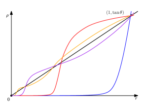
Figure 1. Curves representing analytic solutions

and the boundary of each minimal graph is exactly the graph of $\phi=\tan\theta\cdot f$.

3. Canonical metric on quotient space

According to (2.4), we restrict ourselves to the following $(n+2)$-dimensional smooth submanifold associated to LOMSEs for both Type (I) and Type (II)

(3.1) $$W:=\{(rx,\rho f(x)):\ x\in S^{n},\ r\in\mathbb{R}_{+},\ \rho\in\mathbb{R}\}$$

in $\mathbb{R}^{m+n+2}$.

Every smooth function $\rho(r)$ (or more generally, a parametric curve with nowhere vanishing velocity in the $r\rho$-plane) would give an embedded (or immersed) hypersurface in $W$. Stimulated by the ideas of [Bro66, HL71, Law72] for submanifolds of low cohomogeneity, we consider the right half $r\rho$-plane as the “quotient space” of $W$. Namely, the quotient space only reads off values $(r,\rho)$ for points in $W$.

Proposition 3.1.

With respect to canonical metric

(3.2) $$g_{0}:=\sigma_{0}^{2}\cdot g=\sigma_{0}^{2}\cdot\left[\left(r^{2}+\lambda^{2}\rho^{2}\right)^{p}\cdot r^{2(n-p)}\right]\cdot[dr^{2}+d\rho^{2}]$$

where $\sigma_{0}$ is the volume of the $n$-dimensional unit sphere, the length of every curve equals the volume of corresponding hypersurface in $W\subset\mathbb{R}^{m+n+2}$.

Proof..

Note that this situation is similar to the cohomogeneity one case. We only need to figure out the volume function $V(r,\rho)$ of the $n$-dimensional submanifold corresponding to $(r,\rho)$. Then

$$g_{0}=\big{(}V(r,\rho)\big{)}^{2}\cdot\left[dr^{2}+d\rho^{2}\right]$$

will have the desired property.

For expression of $V(r,\rho)$, let us fix a point $x\in S^{n}$ and choose an orthonormal frame $\{e_{1},\cdots,e_{p},\ e_{p+1},\cdots,e_{n}\}$ of $T_{x}S^{n}$ such that $\{f_{*}(e_{1}),\cdots,\ f_{*}(e_{p})\}$ form an orthogonal set in $T_{f(x)}S^{m}$ of length $\lambda$ and $f_{*}(e_{p+1})=\cdots=f_{*}(e_{n})=0$, by Definition 2.3. Set $f_{i}=\frac{f_{*}(e_{i})}{\lambda}$ for $i=1,\cdots,p$. Hence, the differential $DF_{x}$ for $F(x)=(rx,\rho f(x))$ sends

$$e_{i} \longmapsto (re_{i},\ \lambda\rho f_{i}),\quad 1\leq i\leq p$$

$$e_{j} \longmapsto (re_{j},\ 0),\quad p+1\leq j\leq n.$$

Thus,

$$V(r,\rho) = \int_{F(S^{n})}dv_{F(S^{n})}=\int_{S^{n}}\sqrt{\det(DF^{T}\cdot DF)}dv_{S^{n}}$$

$$= \int_{S^{n}}(\sqrt{r^{2}+\lambda^{2}\rho^{2}})^{p}\cdot r^{(n-p)}dv_{S^{n}}$$

$$= \sigma_{0}({r^{2}+\lambda^{2}\rho^{2}})^{\frac{p}{2}}\cdot r^{(n-p)},$$

and the proposition gets proved. ∎

Remark 3.2.

All solution curves exhibited in Figure 1 are geodesics. In particular, $\rho=\tan\theta\cdot r$ is a geodesic with respect to $g$.

4. Geodesic equation and the minimal surface equation

We show in this section that the geodesic equation with respect to the metric

$$g=\left[\left(r^{2}+\lambda^{2}\rho^{2}\right)^{p}\cdot r^{2(n-p)}\right]\cdot[dr^{2}+d\rho^{2}]=u\cdot[dr^{2}+d\rho^{2}]$$

gives rise to the Evolution Equation (2.5).

The formula for the Christoffel symbol of a conformal metric is

$$\tilde{\Gamma}_{ij}^{k}=\Gamma_{ij}^{k}+\frac{1}{2}\Big{(}(\log u)_{i}\delta^{k}_{j}+(\log u)_{j}\delta^{k}_{i}-(\log u)_{k}\delta_{ij}\Big{)}.$$

Direct calculation gives

$$A :=\frac{1}{2}(\log u)_{r}=\frac{(n-p)\lambda^{2}\rho^{2}+nr^{2}}{(\lambda^{2}\rho^{2}+r^{2})r}=\Gamma_{rr}^{r}=\Gamma_{r\rho}^{\rho}=-\Gamma_{\rho\rho}^{r},$$

$$B :=\frac{1}{2}(\log u)_{\rho}=\frac{p\lambda^{2}\rho}{\lambda^{2}\rho^{2}+r^{2}}=-\Gamma_{rr}^{\rho}=\Gamma_{r\rho}^{r}=\Gamma_{\rho\rho}^{\rho}.$$

Let the arc-length parameter be $s$, and assume $r=r(s)$, $\rho=\rho(s)$ to be a geodesic. Denote $\dot{r}=\dfrac{dr}{ds}$, $\dot{\rho}=\dfrac{d\rho}{ds}$. The geodesic equation is then

$$\ddot{r}+A\dot{r}^{2}+2B\dot{r}\dot{\rho}-A\dot{\rho}^{2}=0,$$

$$\ddot{\rho}-B\dot{r}^{2}+2A\dot{r}\dot{\rho}+B\dot{\rho}^{2}=0.$$

Since $\rho_{r}=\dfrac{\dot{\rho}}{\dot{r}},$ it follows that

$$\rho_{rr} =\frac{\ddot{\rho}\dot{r}-\dot{\rho}\ddot{r}}{\dot{r}^{3}}$$

$$=B-A\rho_{r}+B\rho_{r}^{2}-A\rho_{r}^{3}$$

$$=(1+\rho_{r}^{2})(B-A\rho_{r})$$

which can be verified to be (2.5).

Furthermore, we remark that a rescaling of a geodesic is again geodesic.

5. Computations on stability and instability

In [XYZ18] it has been shown that every LOC of $(n,p,2)$-type (subset of Type (I)) is area-minimizing, thus stable minimal; whereas LOCs for Type (II) LOMSEs are not area-minimizing. The lengths of the solution geodesics (with more and more oscillations) in Figure 1 increase to that of the LOC segment connecting the origin and $(1,\tan\theta)$ (open at the origin and closed at the other side). However, these geodesics are isolated, not forming a continuous family of geodesics. So it was unclear if an LOC segment for Type (II) is stable or not. In this section, we determine stability and instability of these LOC segments in the quotient spaces.

Theorem 5.1.

The LOC segment for an LOMSE is stable if and only if it is of Type (I) and unstable if and only if it is of Type (II).

Remark 5.2.

Theorems 1.1 and 1.2 are corollaries.

Proof..

The strategy is to study the Jacobi field equation. We shall show that an LOC segment $\{(r,\tan\theta\cdot r):r\in(0,1]\}$ contains conjugate points to the point $(1,\tan\theta)$ for Type (II) and no conjugate points for Type (I).

Let us first consider the Gaussian curvature $K$ for metric $g$ in Proposition 3.1 (ignoring the factor $\sigma_{0}$). A well-known formula for Gaussian curvature for isothermal metric $h(dr^{2}+d\rho^{2})$ is

$$K=-\dfrac{1}{2h}\triangle\log h.$$

By $h=\left(r^{2}+\lambda^{2}\rho^{2}\right)^{p}\cdot r^{2(n-p)}$, it becomes

$$K = -\dfrac{1}{2(r^{2}+\lambda^{2}\rho^{2})^{p}\cdot r^{2(n-p)}}\triangle\left(p\log(r^{2}+\lambda^{2}\rho^{2})+2(n-p)\log r\right)$$

$$= \dfrac{1}{(r^{2}+\lambda^{2}\rho^{2})^{p}\cdot r^{2(n-p)}}\left[\dfrac{n-p}{r^{2}}-p(\lambda^{2}-1)\dfrac{r^{2}-\lambda^{2}\rho^{2}}{(r^{2}+\lambda^{2}\rho^{2})^{2}}\right].$$

Along the geodesic $\{\rho=\tan\theta\cdot r\}$,

(5.1) $$K(r)=\dfrac{1}{(1+\lambda^{2}\tan^{2}\theta)^{p}\cdot r^{2(n+1)}}\left[(n-p)-\dfrac{p(\lambda^{2}-1)}{(1+\lambda^{2}\tan^{2}\theta)^{2}}\left(1-\lambda^{2}\tan^{2}\theta\right)\right].$$

To simplify the above expression, we transform (2.2) for LOMSE

(5.2) $$\dfrac{n-p}{\cos^{2}\theta}+\dfrac{p}{\cos^{2}\theta+\lambda^{2}\sin^{2}\theta}=n$$

(by splitting $n=(n-p)+p$) to

$$\dfrac{(n-p)\sin^{2}\theta}{\cos^{2}\theta}+\dfrac{p(\sin^{2}\theta-\lambda^{2}\sin^{2}\theta)}{\cos^{2}\theta+\lambda^{2}\sin^{2}\theta}=0,$$

which implies

(5.3) $$(n-p)=\dfrac{p(\lambda^{2}-1)}{1+\lambda^{2}\tan^{2}\theta}.$$

Now (5.1) gives

(5.4) $$\begin{split}K(r)&=\dfrac{n-p}{(1+\lambda^{2}\tan^{2}\theta)^{p}\cdot r^{2(n+1)}}\left[1-\frac{1-\lambda^{2}\tan^{2}\theta}{1+\lambda^{2}\tan^{2}\theta}\right]\\ &=\dfrac{2(n-p)}{(1+\lambda^{2}\tan^{2}\theta)^{p}\cdot r^{2(n+1)}}\left[1-\frac{1}{1+\lambda^{2}\tan^{2}\theta}\right].\end{split}$$

For solutions to the Jacobi equation, we need the arc-length parameter

(5.5) $$s = \int_{0}^{r}(1+\lambda^{2}\tan^{2}\theta)^{\frac{p}{2}}r^{n}\cdot\sqrt{1+\tan^{2}\theta}\ dr$$

$$= \dfrac{\sqrt{1+\tan^{2}\theta}\ (1+\lambda^{2}\tan^{2}\theta)^{\frac{p}{2}}}{n+1}\cdot r^{n+1}.$$

Therefore

$$K(s) = \dfrac{2(n-p)(1+\tan^{2}\theta)}{(n+1)^{2}s^{2}}\left[1-\frac{1}{1+\lambda^{2}\tan^{2}\theta}\right].$$

Note that (5.3) implies

$$1-\frac{1}{1+\lambda^{2}\tan^{2}\theta} =\frac{p\lambda^{2}-n}{p(\lambda^{2}-1)}$$

$$\text{and}\quad\quad 1+\tan^{2}\theta =\frac{n(\lambda^{2}-1)}{\lambda^{2}(n-p)}.$$

So

$$K(s)=\frac{2(p\lambda^{2}-n)n}{p\lambda^{2}(n+1)^{2}s^{2}}=\dfrac{2(k^{2}+kn-k-n)n}{(k+n-1)k(n+1)^{2}}\cdot\dfrac{1}{s^{2}},$$

according to (2.3).

Define

(5.6) $$a:=\dfrac{2(k^{2}+kn-k-n)n}{(k+n-1)k(n+1)^{2}}.$$

Fix a unit normal vector field $N$ along the LOC segment. Then $J(s)N$ is a Jacobi vector field if and only if

$$J^{\prime\prime}(s)+K(s)J(s)=0.$$

This is a Euler equation. Consider $J(s)=s^{l}$. Then

$$l(l-1)+a=0,$$

and the solutions are

(5.7) $$J(s)=C_{1}e^{\frac{1+\sqrt{\triangle}}{2}\log s}+C_{2}e^{\frac{1-\sqrt{\triangle}}{2}\log s}.$$

(A). When $\triangle=1-4a>0$, all solutions $J(s)=C_{1}s^{\frac{1+\sqrt{\triangle}}{2}}+C_{2}s^{\frac{1-\sqrt{\triangle}}{2}}$ are linear combinations of two power functions whose exponents are distinct real numbers. Apparently for $J$ to vanish at two distinct $s_{1},s_{2}>0$, we must have $C_{1}=C_{2}=0$. Hence the index of the LOC segment is zero and the segment is stable. Similarly, when $\Delta=0$, then $J(s)=C_{1}\sqrt{s}+C_{2}\sqrt{s}\log s$ can not vanish at two distinct $s_{1},s_{2}$ unless it is trivial.

(B). When $\triangle=1-4a<0$, all solutions are

$$J(s)=C_{1}\sqrt{s}\cos\left(\dfrac{\sqrt{-\triangle}}{2}\log s\right)+C_{2}\sqrt{s}\sin\left(\dfrac{\sqrt{-\triangle}}{2}\log s\right).$$

It is clear that there are infinitely many conjugate points to any point on the LOC segment. Therefore, the LOC segment is unstable.

Now let us consider (A) first by solving

$$a=\dfrac{2(k^{2}+kn-k-n)n}{(k+n-1)k(n+1)^{2}}<\dfrac{1}{4}$$

which is equivalent to

$$8n(k^{2}+kn-k-n) < (k+n-1)k(1+n)^{2}$$

$$\Longleftrightarrow\ \ 8nk^{2}+8n(n-1)k-8n^{2} < k^{2}(1+n)^{2}+k(n-1)(n+1)^{2}$$

and further transformed to

$$((1+n)^{2}-8n)k^{2}+k(n-1)[(n+1)^{2}-8n]+8n^{2} > 0$$

(5.8) $$\Longleftrightarrow\quad(n^{2}-6n+1)k^{2}+k(n-1)(n^{2}-6n+1)+8n^{2} > 0$$

If $n\geq 6$, then the leading coefficient of $k^{2}$ is positive and (5.8) holds for all positive $k$. Note that positive integer $n$ has to be odd as the dimension of source space of an Hopf fibration and positive integer $k$ is always even (see Remark 2.5). Direct computation shows that for $n=5$ the solutions are $k=2,4$; for $n=3$ the only solution is $k=2$. It turns out that $a=\frac{1}{4}$ has no solution in our situation.

Therefore, the solution situation of (B) is exactly the opposite to (A).

By comparing with the $(n,k)$ values of Type (I) and Type (II), we have shown that the LOC segment is stable if and only if it is of Type (I); and unstable if and only if it is of Type (II). ∎

Remark 5.3.

As pointed out in [Sim68], in general a (compactly supported) Jacobi field along a surface can not generate a family of nearby minimal surfaces correspondingly. In our case, the Jacobi field along the LOC segment has a lifting to an “upstair” Jacobi field along the regular part of the minimal cone LOC in the Euclidean space, and it can produce a family of nearby minimal surfaces by lifting geodesics around the LOC segment.

6. Some remarks on instability

In this section, we further discuss the close relationship of above calculations with that in [XYZ19], where conditions for Type (II) Lawson-Osserman cones were discovered. The Jacobi field method here is derived from the linearization of geodesic equation; while, in [XYZ19], the ODE requirement (2.5) for a minimal surface is transformed to a dynamic system with linearization analysis at a fixed point that corresponds to the LOC. We shall see that the periods of Jacobi fields observed in current paper coincide with those of dynamic behaviors in [XYZ19], and moreover, we shall establish an explicit translation between these two perspectives.

By (5.5), the arc-length $s$ is a constant multiple of $r^{n+1}$. Therefore, solution (5.7) in variable $r$ becomes

(6.9) $$J(r)=\tilde{C}_{1}e^{\frac{1+\sqrt{\Delta}}{2}(n+1)\log r}+\tilde{C}_{2}e^{\frac{1-\sqrt{\Delta}}{2}(n+1)\log r}.$$

From (5.6), the solutions are linear combinations of

(6.10) $$\exp\left(\frac{1}{2}\bigg{(}(n+1)\pm\sqrt{(n+1)^{2}+8n\Big{(}\frac{n}{k(n+k-1)}-1\Big{)}}\bigg{)}\log r\right).$$

In [XYZ19], the ODE (2.5) for minimal graphs is rewritten as

(6.11) $$\left\{\begin{array}[]{ll}\varphi_{t}=\psi,\\ \psi_{t}=-\psi-\Big{[}\big{(}n-p+\frac{p}{1+\lambda^{2}\varphi^{2}}\big{)}\psi+\big{(}n-p+\frac{(1-\lambda^{2})p}{1+\lambda^{2}\varphi^{2}}\big{)}\varphi\Big{]}\big{[}1+(\varphi+\psi)^{2}\big{]}.\end{array}\right.$$

in variables

$$t:=\log r,\quad\varphi:=\frac{\rho}{r},\quad\psi:=\varphi_{t}.$$

Then the point $(\varphi,\psi)=(\tan\theta,0)$ is a stationary point of the ODE system. Denoting

$$\varphi_{0}=\tan\theta=\sqrt{\dfrac{p-n\lambda^{-2}}{n-p}},$$

the linearization of the ODE system at the point is

$$\begin{pmatrix}(\phi-\varphi_{0})_{t}\\ \psi_{t}\end{pmatrix}=B\begin{pmatrix}(\phi-\varphi_{0})\\ \psi\end{pmatrix},\quad B=\begin{pmatrix}0&1\\ 2n\big{(}\frac{n}{k(k+n-1)}-1\big{)}&-(n+1)\end{pmatrix}.$$

The eigenvalues of $B$ are the solutions of

$$\lambda^{2}+(n+1)\lambda-2n\Big{(}\frac{n}{k(k+n-1)}-1\Big{)}=0$$

and hence are

(6.12) $$\lambda_{1,2}={\frac{1}{2}\bigg{(}-(n+1)\pm\sqrt{(n+1)^{2}+8n\Big{(}\frac{n}{k(k+n-1)}-1}\Big{)}}\bigg{)}.$$

In our case, these two eigenvalues never equal. Therefore, following standard procedure, we use the matrix $P$ of the corresponding eigenvectors to get

$$B=P\begin{pmatrix}\lambda_{1}&\\ &\lambda_{2}\end{pmatrix}P^{-1}.$$

Although $\lambda_{1,2}$ and $P$ may be complex, the product on the right hand side is real. Then every solution to the linearization of system (6.11) at $(\varphi_{0},0)$ is

(6.13) $$P\begin{pmatrix}e^{\lambda_{1}t}&\\ &e^{\lambda_{2}t}\end{pmatrix}P^{-1}\big{(}\vec{v}_{0}-(\varphi_{0},0)\big{)}+(\varphi_{0},0),$$

for some initial point $\vec{v}_{0}$. The product term, a linear combination of

(6.14) $$e^{\lambda t}=\exp\left({\frac{1}{2}\bigg{(}-(n+1)\pm\sqrt{(n+1)^{2}+8n\Big{(}\frac{n}{k(k+n-1)}-1\Big{)}}\bigg{)}}\log r\right),$$

is real. We see that when the square root is imaginary, the ODE system has a stable spiral singularity at $(\tan\theta,0)$. This is how [XYZ19] defines Type (II).

The square root term in (6.14) is the same as that in (6.10). This explains the coincidence of the periodicity. Furthermore, for a more clear correspondance on the instability of Type (II) Lawson-Osserman cones, we shall give an explicit translation from (6.14) to (6.10) to show the intimate connection.

Theoretically, it is well known that (6.9) is obtained by linearization along $\{\rho=\varphi_{0}r\}$; while (6.13) is gained by linearization at $(\varphi_{0},0)$ exactly corresponding to the LOC curve $\{\rho=\varphi_{0}r\}$. This is the essential reason that makes it possible and natural to derive Jacobi fields from orbits to (6.11) in the $\varphi\psi$-plane around $(\varphi_{0},0)$.

We take $(n,p,k)=(5,4,6)$ for example with

$$B=\begin{pmatrix}0&1\\ -\frac{55}{6}&-6\end{pmatrix},\ \ \ \ \ \lambda_{1,2}=-3\pm\dfrac{i}{\sqrt{6}},\ \ \ \ \ \text{and}$$

$P$ can be chosen to be

$$\begin{pmatrix}\dfrac{1}{-3+\frac{i}{\sqrt{6}}}&\dfrac{1}{-3-\frac{i}{\sqrt{6}}}\\ &\\ 1&1\end{pmatrix}.$$

Based on (6.13), the orbit through point $(\varphi_{0},-\epsilon)$ is

$$\begin{pmatrix}e^{-3t}\left(3\sqrt{6}\sin\dfrac{t}{\sqrt{6}}+\cos\dfrac{t}{\sqrt{6}}\right)&\sqrt{6}e^{-3t}\sin\dfrac{t}{\sqrt{6}}\\ &\\ -\dfrac{55}{6}\sqrt{6}e^{-3t}\sin{\dfrac{t}{\sqrt{6}}}&e^{-3t}\left(3\sqrt{6}\sin\dfrac{t}{\sqrt{6}}-\cos\dfrac{t}{\sqrt{6}}\right)\end{pmatrix}\cdot\begin{pmatrix}0\\ \\ -\epsilon\end{pmatrix}+\begin{pmatrix}\varphi_{0}\\ \\ 0\end{pmatrix}.$$

Although the above expression is an approximate orbit to system (6.11), it is exactly what we need to consider in the limiting procedure. Note that by setting $r=e^{t}$ one has $\varphi=\varphi_{0}-\epsilon\sqrt{6}e^{-3t}\sin\dfrac{t}{\sqrt{6}}.$ Therefore,

$$\Big{\{}\rho=\varphi r=\varphi_{0}r-\epsilon\dfrac{\sqrt{6}}{r^{2}}\sin\dfrac{\log r}{\sqrt{6}}:\ \epsilon\in\mathbb{R}_{+}\Big{\}}$$

provide a family of approximations of geodesics in $C^{1}$ sense for $\epsilon\rightarrow 0+$ with the following picture

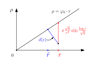
Figure 2. Illustration on the translation back to $r\rho$-plane

which demonstrates $r=\tilde{r}+\dfrac{\varphi_{0}}{\sqrt{1+\varphi_{0}^{2}}}d(\epsilon).$

The Euclidean length of the red vertical segment leads to

(6.15) $$\sqrt{1+\varphi_{0}^{2}}\cdot d(\epsilon)=\epsilon\sqrt{6}\cdot\dfrac{\sin\frac{\log\left(\tilde{r}+\frac{\varphi_{0}}{\sqrt{1+\varphi_{0}^{2}}}d(\epsilon)\right)}{\sqrt{6}}}{\left(\tilde{r}+\frac{\varphi_{0}}{\sqrt{1+\varphi_{0}^{2}}}d(\epsilon)\right)^{2}},$$

and further, the derivative of the expression in $\epsilon$ at zero gives

(6.16) $$\sqrt{1+\varphi_{0}^{2}}\cdot d^{\prime}(0)=\sqrt{6}\cdot\frac{\sin\frac{\log\tilde{r}}{\sqrt{6}}}{\tilde{r}^{2}}.$$

Assume that $N$ is the pointing downward unit normal vector field along $\{\rho=\varphi_{0}r\}$. By the formulation of $g_{0}$ in (3.2), its Euclidean length is of order $-5$ in $\tilde{r}$. Hence, by virtue of the $C^{1}$ approximation, it produces the Jacobi field

(6.17) $$d^{\prime}(0)=\left(C\tilde{r}^{3}\sin\frac{\log\tilde{r}}{\sqrt{6}}\right)N,\text{ for some constant }C.$$

Moreover, if at the beginning we set $r=e^{t-\frac{\sqrt{6}\pi}{2}}$ instead, then (6.17) becomes

(6.18) $$\tilde{d}^{\prime}(0)=\left(\tilde{C}\tilde{r}^{3}\cos\frac{\log\tilde{r}}{\sqrt{6}}\right)N,\text{ for some constant }\tilde{C}.$$

In such way, we see that linear combinations of (6.17) and (6.18) exhaust all Jacobi fields (6.9) for this concrete example.

In general, the same conclusion can also be obtained similarly. Assume that

$$P=\begin{pmatrix}p_{11}&p_{12}\\ &\\ p_{21}&p_{22}\end{pmatrix}\ \ \text{ and }\ \ P^{-1}=\begin{pmatrix}p^{*}_{11}&p^{*}_{12}\\ &\\ p^{*}_{21}&p^{*}_{22}\end{pmatrix}=\dfrac{1}{\det P}\begin{pmatrix}p_{22}&-p_{12}\\ &\\ -p_{21}&p_{11}\end{pmatrix}.$$

Now the approximate orbit through $(\varphi_{0},-\epsilon)$ is

$$P\begin{pmatrix}e^{\lambda_{1}t}&\\ &\\ &e^{\lambda_{2}t}\end{pmatrix}P^{-1}\cdot\begin{pmatrix}0\\ \\ -\epsilon\end{pmatrix}+\begin{pmatrix}\varphi_{0}\\ \\ 0\end{pmatrix}=\begin{pmatrix}\varphi_{0}\\ \\ 0\end{pmatrix}-\epsilon\begin{pmatrix}e^{\lambda_{1}t}p_{11}p^{*}_{12}+e^{\lambda_{2}t}p_{12}p^{*}_{22}\\ \\ e^{\lambda_{1}t}p_{21}p^{*}_{12}+e^{\lambda_{2}t}p_{22}p^{*}_{22}\end{pmatrix}.$$

Hence the corresponding curves in $r\rho$-plane satisfies

(6.19) $$\rho=\big{(}\varphi_{0}-\epsilon(e^{\lambda_{1}t}p_{11}p^{*}_{12}+e^{\lambda_{2}t}p_{12}p^{*}_{22})\big{)}r.$$

By $p_{11}p^{*}_{12}+p_{12}p^{*}_{22}=0$ and (6.12), we have

$$\rho =\big{(}\varphi_{0}-\epsilon p_{11}p^{*}_{12}(e^{\lambda_{1}t}-e^{\lambda_{2}t})\big{)}r$$

$$=\Big{(}\varphi_{0}-\epsilon p_{11}p^{*}_{12}(2e^{\text{Re }\lambda_{1}t}\sin(\text{Im }\lambda_{1}t)i\big{)}\Big{)}r$$

$$=\Big{(}\varphi_{0}+\epsilon\frac{p_{11}p_{12}}{\det P}(2e^{\text{Re }\lambda_{1}t}\sin(\text{Im }\lambda_{1}t)i\big{)}\Big{)}r.$$

We claim that $\frac{p_{11}p_{12}}{\det P}i$ is a real nonzero number. Note that

$$\det\begin{pmatrix}p_{11}&\overline{p_{11}}\\ &\\ p_{21}&\overline{p_{21}}\end{pmatrix}=2\text{Im }(p_{11}\overline{p_{21}})i,\ \ \text{ and }\ \ \begin{pmatrix}\overline{p_{11}}\\ \\ \overline{p_{21}}\\ \end{pmatrix}=\alpha\cdot\begin{pmatrix}p_{12}\\ \\ p_{22}\end{pmatrix}\ \ \text{ for some }\alpha\neq 0\in\mathbb{C}.$$

So

$$\dfrac{p_{11}p_{12}}{\det P}i =\dfrac{\|p_{11}\|^{2}}{\alpha\det P}i=\dfrac{\|p_{11}\|^{2}}{2\text{Im }(p_{11}\overline{p_{21}})}\in\mathbb{R}.$$

Similar to the preceding example, by employing $r=e^{t}$, we have the following relation for signed $d(\epsilon)$

(6.20) $$\sqrt{1+\varphi_{0}^{2}}\cdot d(\epsilon)=-\dfrac{\epsilon\|p_{11}\|^{2}}{\text{Im }(p_{11}\overline{p_{21}})}\cdot\dfrac{\sin\left(\text{Im }\lambda_{1}\log\left(\tilde{r}+\frac{\varphi_{0}}{\sqrt{1+\varphi_{0}^{2}}}d(\epsilon)\right)\right)}{\left(\tilde{r}+\frac{\varphi_{0}}{\sqrt{1+\varphi_{0}^{2}}}d(\epsilon)\right)^{\frac{n-1}{2}}},$$

Since the Euclidean length of $N$ is of order $-n$ in $r$,

(6.21) $$d^{\prime}(0)=\left(C\tilde{r}^{\frac{n+1}{2}}\sin\big{(}\text{Im }\lambda_{1}\log\tilde{r}\big{)}\right)N,\text{ for some constant }C.$$

By using $r=e^{t-\frac{\pi}{2\text{Im }\lambda_{1}}}$ (which generates a rescaling on the $r\rho$-plane) instead, (6.21) becomes

(6.22) $${\tilde{d}}^{\prime}(0)=\left(\tilde{C}\tilde{r}^{\frac{n+1}{2}}\cos\big{(}\text{Im }\lambda_{1}\log\tilde{r}\big{)}\right)N,\text{ for some constant }\tilde{C}.$$

Thus linear combinations of (6.21) and (6.22) provide all Jacobi fields (6.9).

7. Some remarks on stability

In this section, we shall show that the LOC curve for Type (I) in the quotient space is not merely stable minimal but in fact length-minimizing, namely a ray in the sense of classical Riemannian geometry, in its certain angular neighborhood.

To explain local length-minimality, i.e. being length-minimizing in some neighborhood of the LOC curve, we shall construct a geodesic foliation in some angular neighborhood around the LOC curve.

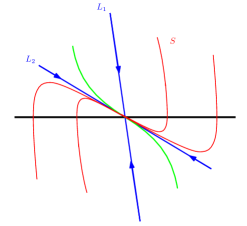
Figure 3. Infinitesimal orbits near $(\varphi_{0},0)$ for Type (I) in the $(\varphi,\psi)$-plane

Note that $\Delta=(n+1)^{2}+8n\big{(}\frac{n}{k(n+k-1)}-1\big{)}>0$. Let $L_{1,2}$ be the line through $(\varphi_{0},0)$ with slopes $\frac{1}{2}[-(n+1)\mp\sqrt{\Delta}]$. Apparently, all orbits accumulate to $L_{2}$ expect one to $L_{1}$ in the infinitesimal model. Hence, starting from $(\varphi_{1},0)$ where $\varphi_{1}$ is sufficiently close to $\varphi_{0}$ and $\varphi_{1}>\varphi_{0}$, there exists an orbit of (6.11) limiting to $(\varphi_{0},0)$ below the $\varphi$-axis with decreasing $\varphi$ values in $(\varphi_{0},\varphi_{1}]$. This orbit corresponds to a geodesic curve $\gamma_{1}$ in the $r\rho$-plane which has strictly decreasing slopes within $(\varphi_{0},\varphi_{1}]$. Similar discussion works for the other side (with $\varphi_{2}<\varphi_{0}$).

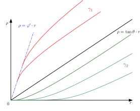
Figure 4. Geodesic foliation around the ray $\rho=\tan\theta\cdot r$

However it is convenient to use the unique orbit from $(0,0)$ to $(\varphi_{0},0)$, i.e., $\varphi_{2}=0$, with increasing $\varphi\in(0,\varphi_{0})$ explored in [XYZ19], which corresponds to a geodesic curve $\gamma_{2}$ in the $r\rho$-plane with strictly increasing slope within $(0,\varphi_{0})$. Thus we can gain a foliation of homothetic geodesics (i.e., obtained by dilations of $\gamma_{1}$ and $\gamma_{2}$) in the angular region $\mathscr{S}$ between $\{\rho=0\}$ and $\{\rho=\varphi_{1}\cdot r\}$.

Therefore, the LOC curve is length-minimizing in the angular region $\mathscr{S}$ following a standard calibration argument (the fundamental theorem of calibrated geometries) using the calibration form $\omega=v\lrcorner\ \tau$ where $v$ is the unit tangent vector fields along the oriented foliation and $\tau$ the oriented unit volume form of $\mathscr{S}$, see [BdGG69, HL82a, HL82b] for details.

References

- [BdGG69] E. Bombieri, E. De Giorgi and E. Giusti: Minimal cones and the Bernstein problem. Invent. Math. 7 (1969), 243–268.
- [BdGM69] E. Bombieri, E. de Giorgi and M. Miranda: Una maggiorazione a priori relativa alle ipersuperfici minimali non parametriche. Arch. Rational Mech. Anal. 32 (1969), 255–267.
- [Bro66] J. Brothers: Integral geometry in homogeneous spaces,. Trans. Amer. Math. Soc. 124 (1966), 480–517.
- [dG57] E. de Giorgi: Sulla differentiabilità e l’analiticità delle estremali degli integrali multipli regolari. Mem. accad. Sci. Torino, s. III, parte I, (1957), 25–43.
- [Dou31] J. Douglas: Solutions of the Problem of Plateau: Trans. Amer. Math. Soc. 33 (1931), 263–321.
- [Fed96] H. Federer: Geometric Measure Theory. Springer-Verlag Berlin Heidelberg, 1996.
- [JS68] H. Jenkins and J. Serrin: The Dirichlet problem for the minimal surface equation in higher dimensions. J. Reine Angew. Math. 229 (1968), 170–187.
- [HL71] W.Y. Hsiang and H. B. Lawson, Jr.: Minimal submanifolds of low cohomogeneity. J. Diff. Geom. 5 (1971), 1–38.
- [HL82a] R. Harvey and H. B. Lawson, Jr.: Calibrated geometries. Acta Math. 148 (1982), 47–157.
- [HL82b] R. Harvey and H. B. Lawson, Jr.: Calibrated Foliations. Amer. J. Math. 104 (1982), 607–633.
- [Law72] H. B. Lawson, Jr.: The Equivariant Plateau Problem and Interior Regularity. Trans. Amer. Math. Soc. 173 (1972), 231–249.
- [LO77] H. B. Lawson, Jr. and R. Osserman: Non-existence, non-uniqueness and irregularity of solutions to the minimal surface system. Acta Math. 139 (1977), 1–17.
- [MT39] M. Morse and C. Tompkins: Existence of minimal surfaces of general critical type. Ann. of Math. 40 (1939), 443–472.
- [Mos60] J. Moser: A new proof of de Giorgi’s theorem concerning the regularity problem for elliptic differential equations. Comm. Pure Appl. Math. 13 (1960), 457–468.
- [Rad30] T. Radó: On Plateau’s problem. Ann. Math. 31 (1930), 457–469.
- [Rad33] T. Radó: On the Problem of Plateau. Ergebnisse der Mathematik und iher Grenzgebiete, Vol. 2, Springer, 1933.
- [Sim68] J. Simons: Minimal varieties in riemannian manifolds. Ann. Math. 88 (1968), 62–105.
- [XYZ19] X. W. Xu, L. Yang and Y. S. Zhang: Dirichlet boundary values on Euclidean balls with infinitely many solutions for the minimal surface system. J.M.P.A. 129 (2019), 266–300.
- [XYZ18] X. W. Xu, L. Yang and Y. S. Zhang: New area-minimizing Lawson-Osserman cones. Adv. Math. 330 (2018), 739–762.
- [Zha1] Y. S. Zhang: On non-existence of solutions of the Dirichlet problem for the minimal surface system, preliminary version available at arXiv:1812.11553.
- [Zha2] Y. S. Zhang: Recent progress on the Dirichlet problem for the minimal surface system and minimal cones, to appear, preliminary version available arXiv:1906.04558.