The Hessian Estimation Evolution Strategy

Abstract

We present a novel black box optimization algorithm called Hessian Estimation Evolution Strategy. The algorithm updates the covariance matrix of its sampling distribution by directly estimating the curvature of the objective function. This algorithm design is targeted at twice continuously differentiable problems. For this, we extend the cumulative step-size adaptation algorithm of the CMA-ES to mirrored sampling. We demonstrate that our approach to covariance matrix adaptation is efficient by evaluating it on the BBOB/COCO testbed. We also show that the algorithm is surprisingly robust when its core assumption of a twice continuously differentiable objective function is violated. The approach yields a new evolution strategy with competitive performance, and at the same time it also offers an interesting alternative to the usual covariance matrix update mechanism.

1 Introduction

We consider minimization of a black-box objective function $f:\mathbb{R}^{d}\to\mathbb{R}$. Modern evolution strategies (ESs) are highly tuned solvers for such problems [7, 6]. The state of the art is marked by the covariance matrix adaptation evolution strategy (CMA-ES) [5, 9] and its many variants.

Most modern evolution strategies (ESs) sample offspring from a Gaussian distribution $\mathcal{N}(m,\sigma^{2}C)$ around a single mean $m\in\mathbb{R}^{d}$. Their most crucial mechanism is adaptation of the step size $\sigma>0$, which enables them to converge at a linear rate on scale-invariant problems [8]. Hence they achieve the fastest possible convergence speed class that can be realized by any comparison-based algorithm [16]. However, for ill-conditioned problems the actual convergence rate can be very slow, i.e., the multiplicative progress per step can be arbitrarily close to one. The main role of CMA is to mitigate this problem: after successful adaptation of the covariance matrix $C$ to a multiple of the inverse of the Hessian $H$ of the problem, the ES makes progress at its optimal rate.

To this end consider a convex quadratic function $f(x)=\frac{1}{2}x^{T}Hx$. Its Hessian matrix $H$ encodes the curvature of the graph of $f$. Knowledge of this curvature is valuable for optimization, e.g., turning a simple gradient step $x\leftarrow x-\eta\cdot\nabla f(x)$ into a Newton step $x\leftarrow x-H^{-1}\nabla f(x)$, which jumps straight into the optimum. For an evolution strategy, adapting $C$ to $H^{-1}$ is equivalent to learning a transformation of the input space that turns a convex quadratic function into the sphere function. This way, after successful adaptation, all convex quadratic functions are as easy to minimize as the sphere function $f(x)=\frac{1}{2}\|x\|^{2}$, i.e., as if the Hessian matrix was $H=I$ (the identity matrix). Due to Taylor’s theorem, the advantage naturally extends to local convergence into twice continuously differentiable local optima, covering a large and highly relevant class of problems.

The usual mechanism for adapting the covariance matrix $C$ of the offspring generating distribution is to change it towards a weighted maximum likelihood estimate of successful steps [9]. The update can equally well be understood as following a stochastic natural gradient in parameter space [13].

In this paper we explore a conceptually different and more direct approach for learning the inverse Hessian. It amounts to estimating the curvature of the objective function on random lines through $m$ by means of finite differences. We design a novel CMA mechanism for updating the covariance matrix $C$ based on the estimated curvature information. We call the resulting algorithm Hessian Estimation Evolution Strategy (HE-ES).

It is worth pointing out that estimating derivatives destroys an important property of CMA-ES, namely invariance under strictly monotonic transformations of objective values. Our new algorithm is still fully invariant under order-preserving affine transformations of objective values. This is an essentially equally good invariance guarantee only in a local situation, namely if the value transformation is well approximated by its first order Taylor polynomial. We address this potential weakness in our experimental evaluation.

The main goals of this paper are

• to present HE-ES and our novel CMA mechanism, and

• to demonstrate its competitiveness with existing algorithms. To this end we compare HE-ES to CMA-ES as a natural baseline. We also compare with NEWUOA [14], which is based directly on iterative estimates of a quadratic model of the objective function. Furthermore, we include BFGS [12], a “work horse” (gradient-based) non-linear optimization algorithm. It is of interest because being a quasi-Newton method, it implicitly estimates the Hessian matrix.

• Finally, we adapt cumulative step size adaptation to mirrored sampling.

The remainder of the paper is structured as follows. In the next section we describe the new algorithm in detail and briefly discuss its relation to CMA-ES. Our main results are of empirical nature, therefore we present a thorough experimental evaluation of the optimization performance of HE-ES and discuss strengths and limitations. We close with our conclusions.

2 The Hessian Estimation Evolution Strategy

The HE-ES algorithm is designed in as close as possible analogy to CMA-ES. Ideally we would change only the covariance matrix adaptation (CMA) mechanism. However, we end up changing also the offspring generation method to a scheme that is tailored to estimating curvature information. In the following we present the algorithm and motivate and detail all mechanisms that deviate from CMA-ES [9].

Estimating Curvature. 

A seemingly natural strategy for estimating the Hessian of an unknown black-box function is to estimate single entries $H_{ij}$ of this $d\times d$ matrix by computing finite differences. For a diagonal entry $H_{ii}$ this requires evaluating three points on a line parallel to the $i$-th coordinate axis, while for an off-diagonal entry $H_{ij}$ we can evaluate four corners of a rectangle with edges parallel to the $i$-th and $j$-th coordinate axis. A serious problem with such a procedure is that entries must remain consistent, which makes it difficult to design an online update of a previous estimate of the matrix. Furthermore, the scheme implies that offspring must be sampled along the coordinate axes, which can significantly impair performance, e.g., on ill-conditioned non-separable problems—which are exactly the problems we would like to excel on.

We therefore propose a different solution. To this end we draw mirrored samples $m\pm v$ and evaluate $f(m+\alpha v)$ for $\alpha\in\{-1,0,+1\}$. Here $v\in\mathbb{R}^{d}$ is the direction of a line through $m$. The length $\|v\|$ of that vector controls the scale on which the finite difference estimate is computed. An estimate of the second directional derivative of $f$ in direction $\frac{v}{\|v\|}$ at $m$ is

$$\frac{f(m+v)+f(m-v)-2f(m)}{\|v\|^{2}}\enspace.$$

For a convex quadratic function $f(x)=\frac{1}{2}(x-x^{*})^{T}H(x-x^{*})$ the above quantity coincides with the directional derivative $\frac{v^{T}Hv}{\|v\|^{2}}$. It can be understood as the “component” of $H$ in direction $\frac{v}{\|v\|}$. The expression simplifies to a diagonal entry $H_{ii}$ if $v$ is a multiple of the $i$-th standard basis vector $e_{i}=(0,\dots,0,1,0,\dots,0)$. For a general twice continuously differentiable function the estimate converges to the above value in the limit $\|v\|\rightarrow 0$. Importantly, $H$ is uniquely determined by these components, so given enough directions $v$ there is no need for a sampling procedure that corresponds to estimating off-diagonal entries $H_{ij}$.

Orthogonal Mirrored Sampling. 

A single pair of mirrored samples provides information on the curvature in a single direction $v$. We learn nothing about the curvature in the $d-1$ dimensional space orthogonal to $v$. To make best use of the available information we should therefore sample the next pair of mirrored samples orthogonal to $v$. We apply the following sampling procedure for random orthogonal directions, which was first proposed in [17]. We draw $d$ Gaussian vectors and record their lengths. The vectors are then orthogonalized with the Gram-Schmidt procedure. Placing the vectors into a $d\times d$ matrix yields an orthogonal matrix uniformly distributed in the orthogonal group $\mathrm{O}(d,\mathbb{R})$. We then rescale the vectors to their original lengths.

1:  input dimension $d$

2:  $z_{1},\dots,z_{d}\sim\mathcal{N}(0,I)$

3:  $n_{1},\dots,n_{d}\leftarrow\|z_{1}\|,\dots,\|z_{d}\|$

4:  apply the Gram-Schmidt procedure to $z_{1},\dots,z_{d}$

5:  return $y_{i}=n_{i}\cdot z_{i},\quad i=1,\dots,d$

Algorithm 1 sampleOrthogonal

The sampling procedure applied for each block is defined in Procedure 1. It is applicable to up to $d$ pairs of mirrored samples. In general we aim to generate $\tilde{\lambda}$ pairs of mirrored samples, which amounts to $\lambda=2\tilde{\lambda}$ offspring in total. We therefore split the pairs into $B=\lceil\tilde{\lambda}/d\rceil$ blocks and apply the above procedure $B$ times. The resulting vectors are denoted as $b_{ij}$, where $i\in\{1,\dots,B\}$ is the block index and $j\in\{1,\dots,d\}$ is the index within each block.

Covariance Matrix Update. 

We aim for an update that modifies an existing covariance matrix in an online fashion. A seemingly straightforward strategy is to adapt the matrix so that after the update it matches the curvature in the sampled directions. This approach is followed in [11], and later in [15]. However, such a strategy disregards the fact that all multiples of the inverse Hessian are optimal covariance matrices. In fact, the update would destroy a perfect covariance matrix simply because it differs from the inverse Hessian by a large factor.

Therefore our goal is to adapt the covariance matrix to the closest multiple of the inverse Hessian $H^{-1}$. To this end we only change curvature values relative to each other: if the measured curvature in direction $v_{1}$ is $10$ times larger than in direction $v_{2}$ then we aim to ensure that the updated matrix represents this relation. Otherwise we modify the matrix as little as possible. In particular, we keep its determinant (encoding the global scale) constant: if an eigenvalue is increased, then another one is decreased accordingly.

The easiest way to achieve the above goals is by means of a multiplicative update [4, 10, 2]. We decompose the covariance matrix into the form $C=A^{T}A$. The mirrored samples take the form $x_{ij}^{\pm}=m\pm\sigma\cdot A\,b_{ij}$, resulting in the curvature estimates $h_{ij}$, which approximate $b_{ij}^{T}A^{T}HA\,b_{ij}$. The update takes the form $A^{\prime}\leftarrow AG$ and hence $C^{\prime}\leftarrow GCG$, where $G$ is a symmetric positive definite matrix.

In the following we apply the above considerations on curvature estimation to the function $\tilde{f}(x)=f\big{(}A(x-m)\big{)}$ using the direction vectors $v=\sigma\cdot b_{ij}$. The actual goal of optimization is to adapt $m$ towards $x^{*}$. Turning $\tilde{f}$ into the sphere function greatly facilitates that process. It is achieved by adapting $A$ towards (a multiple of) any Cholesky factor of $H^{-1}$, or in other words, by making all eigenvalues of $A^{T}HA$ coincide.

In order to understand the update we first review a simplified example. Consider only two vectors $b_{1}$ and $b_{2}$. For simplicity assume that they fulfill $\sigma\|b_{i}\|=1$, and assume that the curvature estimates $h_{ii}$ are exact because the function is convex quadratic. Then the ideal $G$ has an eigenvalue of $\sqrt[4]{h_{22}/h_{11}}$ for eigenvector $b_{1}$, an eigenvalue of $\sqrt[4]{h_{11}/h_{22}}$ for eigenvector $b_{2}$, and eigenvalue $1$ in the space orthogonal to $b_{1}$ and $b_{2}$. This seemingly very specific choice ensures that $\det(G)=1$ and it holds

$$b_{1}^{T}(A^{\prime})^{T}HA^{\prime}\,b_{1} =b_{1}^{T}GA^{T}HAGb_{1}$$

$$=\sqrt{\frac{h_{22}}{h_{11}}}\cdot b_{1}^{T}A^{T}HA\,b_{1}=\sqrt{\frac{h_{22}}{h_{11}}}\cdot h_{11}=\sqrt{h_{11}h_{22}}\enspace,$$

which coincides with $b_{2}^{T}(A^{\prime})^{T}HA^{\prime}b_{2}$ for symmetry reasons. Hence, after the update the curvatures in directions $b_{1}$ and $b_{2}$ have become equal, while all curvatures orthogonal to the sampling directions remain unchanged. In this sense the resulting problem $\tilde{f}$ has come closer to the sphere function.

1:  input $b_{ij}$, $f(m)$, $f(x_{ij}^{\pm})$, $\sigma$

2:  parameters $\kappa$, $\eta_{A}$

3:  $h_{ij}\leftarrow\frac{f(x_{ij}^{+})+f(x_{ij}^{-})-2f(m)}{\sigma^{2}\cdot\|b_{ij}\|^{2}}$ # estimate curvature along $b_{ij}$

4:  if $\max(\{h_{ij}\})\leq 0$ then return $I$

5:  $c\leftarrow\max(\{h_{ij}\})/\kappa$

6:  $h_{ij}\leftarrow\max(h_{ij},c)$ # truncate to trust region

7:  $q_{ij}\leftarrow\log(h_{ij})$

8:  $q_{ij}\leftarrow q_{ij}-\frac{1}{\tilde{\lambda}}\cdot\sum_{ij}q_{ij}$ # subtract mean $\to$ ensure unit determinant

9:  $q_{ij}\leftarrow q_{ij}\cdot\frac{-\eta_{A}}{2}$ # learning rate and inverse square root (exponent $-1/2$)

10:  $q_{B,j}\leftarrow 0\quad\forall j\in\{dB-\tilde{\lambda},\dots,d\}$ # neutral update in the unused directions

11:  return $\frac{1}{B}\sum_{ij}\frac{\exp(q_{ij})}{\|b_{ij}\|^{2}}\cdot b_{ij}b_{ij}^{T}$

Algorithm 2 computeG

A generalization of the above update to an arbitrary number of (unnormalized) update directions $\sigma\cdot b_{ij}$ is implemented by Procedure 2, which computes the matrix $G$. It forms the algorithmic core of our method.

This core works very well, for example, for smooth convex problems. General non-smooth and non-convex objective functions can exhibit unstable curvature estimates $h_{ij}$. A noisy objective function can create similar issues. For non-convex problems, the eigenvalues of a Hessian can be zero or even negative, in contrast to the eigenvalues of a covariance matrix. In all of these situations we are better off to smoothen the update. Therefore procedure 2 takes two measures: first, it bounds the conditioning of the multiplicative update $G$ by a constant $\kappa$ to limit the effect of outliers (lines 5-6), and second it applies a learning rate $\eta_{A}\in(0,1]$ to stabilize estimates through temporal smoothing (line 9). The first of these mechanisms also gracefully handles curvature estimates $h_{ij}\leq 0$ by clipping them to a small positive value. This is a reasonable thing to do since we want to emphasize sampling in these directions without completely destroying the learned information. In our experiments, we use the settings $\kappa=3$ and $\eta_{A}=1/2$. They represent a reasonable compromise between stability and adaptation speed.

Cumulative Step-size Adaptation (CSA) for Orthogonal Frames. 

The usage of mirrored sampling for CSA was previously explored in [3, 17]. It was found that the default algorithm exhibits a strong step size decay on flat or random function surfaces. In the past this issue was alleviated by not considering the mirrored samples from the population when computing the CSA update. This however is inefficient as only half of the samples are used to update the step-size. In this section, we will quantify the step-length bias of CSA with mirrored samples under selection among all offspring. For this, we observe that under mirrored sampling each direction $b_{ij}$ obtains two weights $w_{ij}^{+}$ and $w_{ij}^{-}$ based on the function-values of the mirrored pair $x_{ij}^{\pm}$. Thus, we can write the CSA mean computation [5] as

$$\sum_{i,j}\left(w_{ij}^{+}\frac{A^{-1}(x^{+}_{ij}-m)}{\sigma}+w_{ij}^{-}\frac{A^{-1}(x^{-}_{ij}-m)}{\sigma}\right)=\sum_{i,j}(w_{ij}^{+}-w_{ij}^{-})b_{ij}\enspace,$$ (1)

leading to an update of the evolution path

$$p_{s}^{(t+1)}\leftarrow(1-c_{s})\cdot p_{s}^{(t)}+\sqrt{c_{s}\cdot(2-c_{s})\cdot\mu_{\text{eff}}}\cdot\sum_{ij}(w_{ij}^{+}-w_{ij}^{-})\cdot b_{ij}\enspace.$$ (2)

In the CSA, the evolution path is updated such that its expected length under random selection is the expected value of the $\chi^{2}(d)$ distribution. To correct for the bias introduced by the weighted mean, the CSA adds the correction $\mu_{\text{eff}}=1/\sum_{i}w^{2}_{i}$. In the mirror-sampling case, the subtraction of the weights on the right hand side of (1) means that the expected length of the vector is smaller than expected under non-mirrored sampling, therefore the step-size update is biased and tends to reduce the step-size prematurely. We fix this problem by computing the correct normalization factor $\mu_{\text{eff}}^{\text{mirrored}}>\mu_{\text{eff}}$.

Under random selection, $w_{ij}^{+}$ and $w_{ij}^{-}$ are randomly picked without replacement from $\vec{w}$, independently of $b_{ij}$. Thus, the distribution of the weighted sample-average of (1) is still normal and the expected squared length is:

$$E\left\{\left\lVert\sum_{i,j}(w_{ij}^{+}-w_{ij}^{-})b_{ij}\right\rVert^{2}\right\}=E\left\{\sum_{i,j}(w_{ij}^{+}-w_{ij}^{-})^{2}\right\}E\left\{\lVert y\rVert^{2}\right\}$$

$$=E\left\{\sum_{i,j}(w_{ij}^{+}-w_{ij}^{-})^{2}\right\}d$$

Note that in the first step, we used that $E\left\{y_{i}^{T}y_{j}\right\}=0$ for $i\neq j$, while the second step holds because we ensure during sampling that the squared length of the samples is still $\chi^{2}(d)$-distributed. Next, we will use that the set of all $w_{ij}^{+}$ and $w_{ij}^{-}$ together forms the weight vector $\vec{w}$ and thus the expectation can be written as permutations $\tau$ of the indices of $\vec{w}$. We can therefore write the expectation in terms of $w_{i}$ as:

$$E\left\{\sum_{i,j}^{\tilde{\lambda}}(w_{ij}^{+}-w_{ij}^{-})^{2}\right\} =E\left\{\sum_{i,j}^{\tilde{\lambda}}(w_{ij}^{+})^{2}+(w_{ij}^{-})^{2}-2w_{ij}^{+}w_{ij}^{-}\right\}$$

$$=E_{\tau}\left\{\sum_{k=1}^{\tilde{\lambda}}w_{\tau(k)}^{2}+w_{\tau(k+\tilde{\lambda})}^{2}-2w_{\tau(k)}w_{\tau(k+\tilde{\lambda})}\right\}$$

$$=\frac{1}{\mu_{\text{eff}}}-2E_{\tau}\left\{\sum_{k=1}^{\tilde{\lambda}}w_{\tau(k)}w_{\tau(k+\tilde{\lambda})}\right\}$$

To continue, we expand the expectation and count the number of times each $(w_{i},w_{j})$-pair appears. There is a total of $(2\tilde{\lambda})!$ permutations and for each $(i,j)$-pair with $i\neq j$, there are $(2\tilde{\lambda})!/(2\tilde{\lambda}\cdot(2\tilde{\lambda}-1))$ permutations such that $\tau(k)=i$ and $\tau(k+\tilde{\lambda})=j$ for each $k$, which leads to another factor of $\tilde{\lambda}$. Thus, we obtain:

$$\frac{1}{\mu_{\text{eff}}}-2E_{\tau}\left\{\sum_{k=1}^{\tilde{\lambda}}w_{\tau(k)}w_{\tau(k+\tilde{\lambda})}\right\}=\frac{1}{\mu_{\text{eff}}}-\frac{2}{(2\tilde{\lambda})!}\sum_{i,j\neq i}^{2\tilde{\lambda}}\frac{\tilde{\lambda}(2\tilde{\lambda})!}{2\tilde{\lambda}\cdot(2\tilde{\lambda}-1)}w_{i}w_{j}\\ =\frac{1}{\mu_{\text{eff}}}-\frac{1}{2\tilde{\lambda}-1}\sum_{i,j\neq i}^{2\tilde{\lambda}}w_{i}w_{j}=\frac{1}{\mu_{\text{eff}}}-\frac{1}{2\tilde{\lambda}-1}\sum_{i}^{2\tilde{\lambda}}w_{i}(1-w_{i})\\ =\frac{1}{\mu_{\text{eff}}}-\frac{1}{2\tilde{\lambda}-1}\left(1-\frac{1}{\mu_{\text{eff}}}\right)=\frac{1}{\mu_{\text{eff}}}\left(1-\frac{\mu_{\text{eff}}-1}{2\tilde{\lambda}-1}\right)$$

In the second step, we use $\sum_{j\neq i}^{2\tilde{\lambda}}w_{j}=1-w_{i}$. Thus, we remove the step-length bias in CSA by replacing $\mu_{\text{eff}}$ in equation (2) with

$$\mu_{\text{eff}}^{\text{mirrored}}:=\frac{\mu_{\text{eff}}}{1-\frac{\mu_{\text{eff}}-1}{2\tilde{\lambda}-1}}.$$

The Algorithm. 

1:  input $m^{(0)}\in\mathbb{R}^{d}$, $\sigma^{(0)}>0$, $A^{(0)}\in\mathbb{R}^{d\times d}$

2:  parameters $\tilde{\lambda}\in\mathbb{N}$, $c_{s}$, $d_{s}$, $w\in\mathbb{R}^{2\tilde{\lambda}}$

3:  $B\leftarrow\lceil\tilde{\lambda}/d\rceil$

4:  $p_{s}^{(0)}\leftarrow 0\in\mathbb{R}^{d}$

5:  $g_{s}^{(0)}\leftarrow 0$

6:  $t\leftarrow 0$

7:  repeat

8:     for $j\in\{1,\dots,B\}$ do

9:        $b_{1j},\dots,b_{dj}\leftarrow$ sampleOrthogonal()

10:     $x_{ij}^{-}\leftarrow m^{(t)}-\sigma^{(t)}\cdot A^{(t)}b_{ij}$      for $i+(j-1)B\leq\tilde{\lambda}$

11:     $x_{ij}^{+}\leftarrow m^{(t)}+\sigma^{(t)}\cdot A^{(t)}b_{ij}$      for $i+(j-1)B\leq\tilde{\lambda}$ # mirrored sampling

12:     $A^{(t+1)}\leftarrow A^{(t)}\cdot$ computeG($\{b_{ij}\}$, $f(m)$, $\{f(x_{ij}^{\pm})\}$, $\sigma^{(t)}$) # matrix adaptation

13:     $w_{ij}^{\pm}\leftarrow w_{\text{rank}(f(x_{ij}^{\pm}))}$

14:     $m^{(t+1)}\leftarrow\sum_{ij}w_{ij}^{\pm}\cdot x_{ij}^{\pm}$ # mean update

15:     $g_{s}^{(t+1)}\leftarrow(1-c_{s})^{2}\cdot g_{s}^{(t)}+c_{s}\cdot(2-c_{s})$

16:     $p_{s}^{(t+1)}\leftarrow(1-c_{s})\cdot p_{s}^{(t)}+\sqrt{c_{s}\cdot(2-c_{s})\cdot\mu_{\text{eff}}^{\text{mirrored}}}\cdot\sum_{ij}(w_{ij}^{+}-w_{ij}^{-})\cdot b_{ij}$

17:     $\sigma^{(t+1)}\leftarrow\sigma^{(t)}\cdot\exp\left(\frac{c_{s}}{d_{s}}\cdot\frac{\|p_{s}^{(t+1)}\|}{\chi_{d}}-\sqrt{g_{s}^{(t+1)}}\right)$ # CSA

18:     $t\leftarrow t+1$

19:  until  stopping criterion is met

Algorithm 3 Hessian Estimation Evolution Strategy (HE-ES)

The resulting HE-ES algorithm is summarized in Algorithm 3. Up to the (significant) changes discussed in the previous sections its design is identical to CMA-ES. In particular, it relies on global intermediate recombination, non-elitist selection, cumulative step-size adaptation (CSA), and it applies the same weights as CMA-ES to the offspring [5]. As default number of mirrored directions, we chose $\tilde{\lambda}=2+\lfloor\frac{3}{2}\log(d)\rfloor$. As learning-rates $c_{s}$ and $d_{s}$ of the CSA in HE-ES, we chose the same values as the implementation of the CMA in pycma-2.7.0 with $2\tilde{\lambda}$ offspring. In contrast to CMA-ES, HE-ES needs to evaluate $f(m)$ in each generation. This value is used only for estimating curvatures.

3 Experimental Evaluation

Our experimental evaluation aims to answer the following research questions:

1. Is Hessian estimation a competitive CMA scheme?

2. What are its strengths and weaknesses compared with CMA-ES?

3. How much does performance change under monotonically increasing but non-affine fitness transformations?

The source code of the algorithm that was used in all experiments is available from the first author’s website.

Benchmark Study. 

Our first experiment is to run the standardized BBOB/COCO procedure, which tests the algorithm on 15 instances of 24 benchmark problems [6]. For handling multi-modal problems we equip HE-ES with an IPOP restart mechanism [1], which restarts the algorithm with doubled population size as soon the standard deviation of the fitness values of a generation falls below $10^{-9}$.

The BBOB platform generates a plethora of results. Due to space constraints we show a representative subset thereof. Figures 1 and  2 show ECDF plots on all 24 function for problem dimension 20, with IPOP-CMA-ES, BFGS, and NEWUOA as baselines. Figure 3 shows overall performance in dimensions 2, 5, 10, and 20. The results for IPOP-CMA-ES, BFGS, and NEWUOA were obtained from the BBOB/COCO platform.

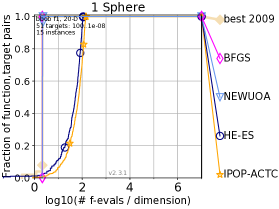
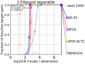
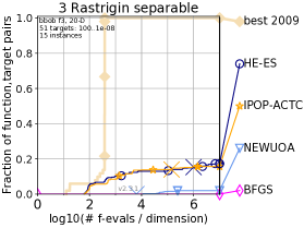
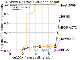
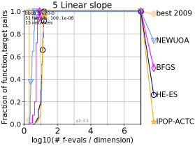
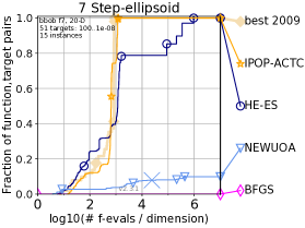
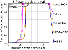
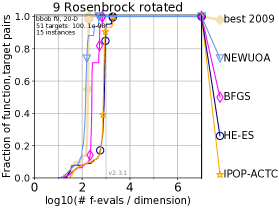
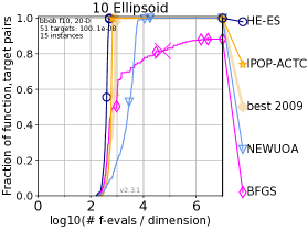
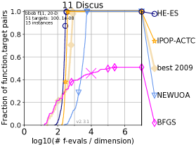
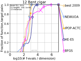
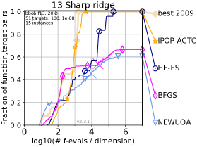
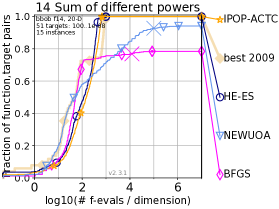
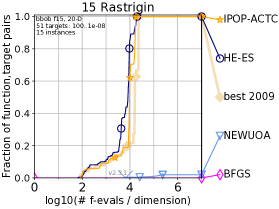
Figure 1: ECDF plots for the noiseless BBOB problems 1–15 in dimension $d=20$. We generally observe that HE-ES performs very well on smooth unimodal problems (functions 1, 2, 5, 8, 9, 10, 11, 12, 14).

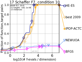
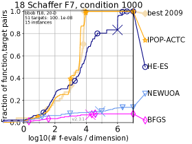
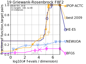
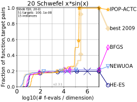
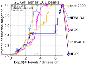
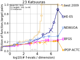
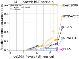
Figure 2: ECDF plots for the noiseless BBOB problems 16–24 in dimension $d=20$.

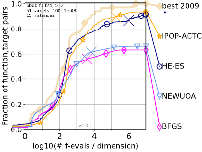
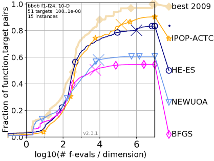
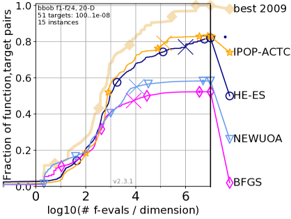
Figure 3: Aggregated performance on all 24 BBOB functions in dimensions 2, 5, 10 and 20. We observe that HE-ES clearly outperforms NEWUOA and BFGS. IPOP-CMA-ES is more reliable then HE-ES, and this gap slightly increases with increasing dimension. The differences mostly originate from hard multi-modal problems.

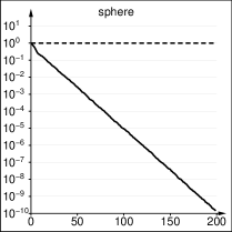
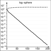
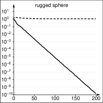
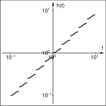
Figure 4: Distance to the optimum (solid) and condition number of $C$ (dashed) over 200 generations of HE-ES started at $m=(1,0,\dots,0)\in\mathbb{R}^{10}$ with $\sigma=0.1$ for sphere, log-sphere, and rugged sphere. The curves are medians over 99 independent runs. Right: log-log plot of the transformation $h$.

Discussion. 

We observe excellent performance across most problems. On all convex quadratic problems ($f_{1}$, $f_{2}$, $f_{10}$, $f_{11}$, $f_{12}$) HE-ES performs very well, and on $f_{10}$ (ellipsoid) and $f_{11}$ (discus) it even outperforms the hypothetical “2009-best portfolio algorithm”, which picks the best optimizer from the 2009 competition for each problem. Surprisingly, the same holds for problems $f_{15}$ (Rastrigin), $f_{16}$ (Weierstraß, see below), $f_{17}$ (Schaffer F7, condition 10), and $f_{19}$ (Griewank-Rosenbrock). Overall, the performance is much closer to CMA-ES than to NEWUOA and BFGS, which indicates that the character of an ES is preserved, despite the novel mechanism for updating the covariance matrix.

Compared to IPOP-CMA-ES, we observe degraded performance on $f_{6}$ (attractive sector), $f_{13}$ (sharp ridge), $f_{20}$ (Schwefel $x\cdot\sin(x)$), $f_{21}$ and $f_{22}$ (Gallagher peaks), $f_{23}$ (Katsuuras), and $f_{24}$ (Lunacek bi-Rastrigin). HE-ES apparently struggles with the asymmetry of the attractive sector problem, which can yield drastically wrong curvature estimates. Similarly, it is conceivable that estimating curvatures on the sharp ridge problem is prone to failure. We believe that these two benchmark functions highlight inherent limitations of the HE-ES update.

Control Experiments. 

In order to understand the weak performance on the highly multi-modal problems despite IPOP restarts we investigated the behavior of HE-ES on the deceptive Lunacek problem $f_{24}$ in dimension $d=10$. We ran HE-ES with IPOP restarts 100 times with a reduced budget of $10^{4}\cdot d$ function evaluations. This medium-sized budget is $100$ times smaller than in the BBOB/COCO experiments. It suffices for 4 to 5 runs, with population sizes ranging from $10$ to $160$. We found that HE-ES converged to the better of the two funnels in 83 cases, and solved the problem to a high precision of $10^{-10}$ in 40 out of 100 cases, which corresponds to reaching all BBOB targets. This means that the correct funnel and the best local optimum of the Rastrigin structure were found in $40\%$ of the cases, which is a quite satisfactory behavior. It is noteworthy that CMA mechanisms are not even needed for this problem (indeed, performance is unchanged when disabling CMA), and hence the performance difference to CMA-ES is probably an artifact of a different restart implementation. This is unrelated to the new CMA mechanism and hence of minor relevance for our investigation.

As mentioned above, HE-ES performs surprisingly well on the Weierstraß function $f_{16}$, which is continuous but nowhere differentiable, and therefore strongly violates the assumption of a twice continuously differentiable objective function. At first glance, this result is surprising. The reason is that HE-ES does not really need correct estimates of the curvature. It is only relevant that the structure (the “global trend”) of the objective function at the relevant scale (given by $\sigma$) is correctly captured. Of course, HE-ES picks up misleading curvature information. However, since the Weierstraß function does not exhibit a systematic preference for a particular direction, such unhelpful information averages out over time and hence does not have a lasting detrimental effect.

In order to investigate this effect closer we performed the following experiment. We start from the 10-dimensional sphere function $f(x)=\frac{1}{2}\|x\|^{2}$ as a base case. Then we create two variants by monotonically transforming the function values, leaving the level sets intact, resulting in the non-convex function $\log(f(x))$ (log-sphere), and the rugged and discontinuous function $h(f(x))$ with $h(t)=\exp\left(\left[\frac{1}{4}-\frac{1}{2}\cos(\pi(5\log(t)-r(t)))+r(t)\right]/5\right)$, where $r(t)=\lfloor 5\log(t)\rfloor$ (rugged sphere). Figure 4 shows a plot of the transformation $h$ as well as the resulting optimization performance of HE-ES. For sphere the condition number remains at exactly one (the optimal value). Importantly, in the other cases the condition number remains close enough to one so as to not impair optimization performance. For the log-sphere there is a slowdown, however, of negligible magnitude: HE-ES requires about $5\%$ more time. We observe that in this setup, surprisingly, HE-ES suffers nearly not at all from misleading curvature estimates.

4 Conclusion

We have presented the Hessian Estimation Evolution Strategy (HE-ES), an ES with a novel covariance matrix adaptation mechanism. It adapts the covariance matrix towards the inverse Hessian projected to random lines, estimated through finite differences by means of mirrored sampling. The algorithm comes with a specialized cumulative step size adaptation rule for mirrored sampling.

Despite its seemingly strong assumptions the method works well on a broad range of problems. It is particularly well suited for smooth unimodal problems like convex quadratic functions and the Rosenbrock function. Surprisingly, the adaptation mechanism that is based on estimating presumedly positive second derivatives can work well on non-convex and even on discontinuous problems.

We believe that the HE-ES offers an interesting alternative to adapting the covariance matrix of the sampling distribution towards the maximum likelihood estimator of successful steps, corresponding to the natural gradient in parameter space.

References

- [1] Auger, A., Hansen, N.: A restart CMA evolution strategy with increasing population size. In: IEEE Congress on Evolutionary Computation. vol. 2, pp. 1769–1776 (2005)
- [2] Beyer, H.G., Sendhoff, B.: Simplify your covariance matrix adaptation evolution strategy. IEEE Transactions on Evolutionary Computation 21(5), 746–759 (2017)
- [3] Brockhoff, D., Auger, A., Hansen, N., Arnold, D.V., Hohm, T.: Mirrored sampling and sequential selection for evolution strategies. In: International Conference on Parallel Problem Solving from Nature. pp. 11–21. Springer (2010)
- [4] Glasmachers, T., Schaul, T., Sun, Y., Wierstra, D., Schmidhuber, J.: Exponential Natural Evolution Strategies. In: Genetic and Evolutionary Computation Conference (GECCO). pp. 393–400. ACM (2010)
- [5] Hansen, N., Ostermeier, A.: Completely derandomized self-adaptation in evolution strategies. Evolutionary Computation 9(2), 159–195 (2001)
- [6] Hansen, N., Auger, A., Mersmann, O., Tušar, T., Brockhoff, D.: COCO: A platform for comparing continuous optimizers in a black-box setting. Tech. Rep. 1603.08785, arXiv.org (2016)
- [7] Hansen, N., Auger, A., Ros, R., Finck, S., Pošík, P.: Comparing results of 31 algorithms from the black-box optimization benchmarking BBOB-2009. In: Proceedings of the 12th annual conference companion on Genetic and evolutionary computation. pp. 1689–1696 (2010)
- [8] Jebalia, M., Auger, A.: Log-linear convergence of the scale-invariant (/ w, )-es and optimal for intermediate recombination for large population sizes. In: International Conference on Parallel Problem Solving from Nature. pp. 52–62. Springer (2010)
- [9] Kern, S., Müller, S.D., Hansen, N., Büche, D., Ocenasek, J., Koumoutsakos, P.: Learning probability distributions in continuous evolutionary algorithms–a comparative review. Natural Computing 3(1), 77–112 (2004)
- [10] Krause, O., Glasmachers, T.: A CMA-ES with multiplicative covariance matrix updates. In: Proceedings of the Genetic and Evolutionary Computation Conference (GECCO) (2015)
- [11] Leventhal, D., Lewis, A.: Randomized hessian estimation and directional search. Optimization 60(3), 329–345 (2011)
- [12] Nocedal, J., Wright, S.: Numerical optimization. Springer (2006)
- [13] Ollivier, Y., Arnold, L., Auger, A., Hansen, N.: Information-geometric optimization algorithms: A unifying picture via invariance principles. The Journal of Machine Learning Research 18(1), 564–628 (2017)
- [14] Powell, M.: The NEWUOA software for unconstrained optimization without derivatives. Tech. Rep. DAMTP 2004/NA05, Department of Applied Mathematics and Theoretical Physics, Cambridge University (2004)
- [15] Stich, S.U., Müller, C.L., Gärtner, B.: Variable metric random pursuit. Mathematical Programming 156(1–2), 549–579 (2016)
- [16] Teytaud, O., Gelly, S.: General lower bounds for evolutionary algorithms. In: Parallel Problem Solving from Nature-PPSN IX, pp. 21–31. Springer (2006)
- [17] Wang, H., Emmerich, M., Bäck, T.: Mirrored orthogonal sampling for covariance matrix adaptation evolution strategies. Evolutionary computation 27(4), 699–725 (2019)