A comparison between the nonlocal and the classical worlds:
minimal surfaces, phase transitions, and geometric flows

The nonlocal world presents an abundance of surprises and wonders to discover. These special properties of the nonlocal world are usually the consequence of long-range interactions, which, especially in presence of geometric structures and nonlinear phenomena, end up producing a variety of novel patterns. We will briefly discuss some of these features, focusing on the case of (non)local minimal surfaces, (non)local phase coexistence models, and (non)local geometric flows.

1 Nonlocal minimal surfaces

In [MR2675483], a new notion of nonlocal perimeter has been introduced, and the study of the corresponding minimizers has started (related energy functionals had previously arisen in [MR1111612] in the context of phase systems and fractals). The simple, but deep idea, grounding this new definition consists in considering pointwise interactions between disjoint sets, modulated by a kernel. The prototype of these interactions considers kernels which have translational, rotational, and dilation invariance. Concretely, given $\sigma\in(0,1)$, one considers the $\sigma$-interaction between two disjoint sets $F$ and $G$ in ${\mathbb{R}}^{n}$ as defined by

$${\mathcal{I}}_{\sigma}(F,G):=\iint_{F\times G}\frac{dx\,dy}{|x-y|^{n+\sigma}},$$ (1)

and the $\sigma$-perimeter of a set $E$ in ${\mathbb{R}}^{n}$ as the $\sigma$-interaction between $E$ and its complement $E^{c}$, namely

$${\rm Per}_{\sigma}(E,{\mathbb{R}}^{n}):={\mathcal{I}}_{\sigma}(E,E^{c}).$$ (2)

To deal with local minimizers, given a domain $\Omega\subset{\mathbb{R}}^{n}$ (say, with sufficiently smooth boundary), it is also convenient to introduce the notion of $\sigma$-perimeter of a set $E$ in $\Omega$. To this end, one can consider the interaction in (2) as composed by four different terms (by considering the intersections of $E$ and $E^{c}$ with $\Omega$ and $\Omega^{c}$), namely we can rewrite (2) as

$$\begin{split}&{\rm Per}_{\sigma}(E,{\mathbb{R}}^{n})={\mathcal{I}}_{\sigma}(E\cap\Omega,E^{c}\cap\Omega)\\ &\quad+{\mathcal{I}}_{\sigma}(E\cap\Omega,E^{c}\cap\Omega^{c})+{\mathcal{I}}_{\sigma}(E\cap\Omega^{c},E^{c}\cap\Omega)\\ &\quad+{\mathcal{I}}_{\sigma}(E\cap\Omega^{c},E^{c}\cap\Omega^{c}).\end{split}$$ (3)

Among the four terms in the right hand side of (3), the first three terms take into account interactions in which at least one contribution comes from $\Omega$ (specifically, all the contributions to ${\mathcal{I}}_{\sigma}(E\cap\Omega,E^{c}\cap\Omega)$ come from $\Omega$, while the contributions to ${\mathcal{I}}_{\sigma}(E\cap\Omega,E^{c}\cap\Omega^{c})$ and ${\mathcal{I}}_{\sigma}(E\cap\Omega^{c},E^{c}\cap\Omega)$ come from the interactions of points in $\Omega$ with points in $\Omega^{c}$). The last term in (3) is structurally different, since it only takes into account contributions coming from outside $\Omega$. It is therefore natural to define the $\sigma$-perimeter of a set $E$ in $\Omega$ as the collection of all the contributions in (3) that take into account points in $\Omega$, thus defining

$$\begin{split}&{\rm Per}_{\sigma}(E,\Omega):={\mathcal{I}}_{\sigma}(E\cap\Omega,E^{c}\cap\Omega)\\ &\quad+{\mathcal{I}}_{\sigma}(E\cap\Omega,E^{c}\cap\Omega^{c})+{\mathcal{I}}_{\sigma}(E\cap\Omega^{c},E^{c}\cap\Omega),\end{split}$$ (4)

see Figure 1

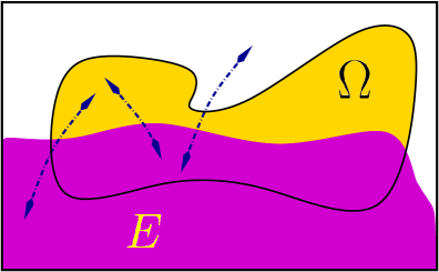
Figure 1: Long-range interactions leading to the fractional perimeter of the set $E$ in $\Omega$.

This notion of perimeter recovers the classical one as $\sigma\nearrow 1$ in various senses, see e.g. [zbMATH02134074, MR1942130, MR2765717, MR2782803, MR3827804], and indeed the analogy between the minimizers of (4) with respect to prescribed sets outside $\Omega$ (named “nonlocal minimal surfaces” in [MR2675483]) and the minimizers of the classical perimeter (the “classical minimal surfaces”) has been widely exploited in [MR2675483] as well in a series of subsequent articles, such as [MR3107529]. Notwithstanding the important similarities between the nonlocal and the classical settings, many striking differences arise, as we will also describe in this note.

Minimizers, and more generally critical points, of the $\sigma$-perimeter satisfy (with a suitable, weak or viscosity, meaning, and in a principal value sense) the equation

$$\begin{split}&{\mathcal{H}}^{\sigma}_{E}(x):=\int_{{\mathbb{R}}^{n}}\frac{\Xi_{E}(y)}{|x-y|^{n+\sigma}}\,dy=0,\\ &\qquad{\mbox{ for }}x\in(\partial E)\cap\Omega,\end{split}$$ (5)

being

$$\Xi_{E}(y):=\begin{cases}-1&{\mbox{ if }}x\in E,\\ 1&{\mbox{ if }}x\in E^{c},\end{cases}$$

see [MR2675483, LUMA]. The quantity ${\mathcal{H}}^{\sigma}_{E}$ can be seen as a “nonlocal mean curvature”, and indeed it approaches in various senses the classical mean curvature ${\mathcal{H}}^{1}_{E}$ (though important differences arise, see [MR3230079]). Interestingly, the nonlocal mean curvature measures the size of $E$ with respect to its complement, in an integral fashion weighted by the interaction kernel, in a precise form given by (5). This interpretation is indeed closely related with the classical mean curvature, in which the size of $E$ is measured only “in the vicinity of the boundary”, since (up to normalizing constants)

$${\mathcal{H}}^{1}_{E}(x)=\lim_{\rho\searrow 0}\frac{1}{\rho^{n+1}}\,\int_{B_{\rho}(x)}\Xi_{E}(y)\,dy,\qquad{\mbox{ for }}x\in\partial E.$$

The settings in (2) and (5) also reveal the “fractional notion” of these nonlocal minimal surfaces. As a matter of fact, if one considers the fractional Gagliardo seminorm defined, for every $s\in(0,1)$, by

$$[f]_{H^{s}({\mathbb{R}}^{n})}:=\sqrt{\iint_{{\mathbb{R}}^{n}\times{\mathbb{R}}^{n}}\frac{|f(x)-f(y)|^{2}}{|x-y|^{n+2s}}\,dx\,dy},$$

it follows that

$$[\Xi_{E}]_{H^{\sigma/2}({\mathbb{R}}^{n})}^{2}=8\,{\rm Per}_{\sigma}(E).$$

Moreover, defining the fractional Laplacian as

$$(-\Delta)^{s}f(x):=\int_{{\mathbb{R}}^{n}}\frac{f(x)-f(y)}{|x-y|^{n+2s}}\,dy,$$

and, for a smooth set $E$, identifying a.e. the function $\Xi_{E}$ with

$$\widetilde{\Xi}_{E}(y):=\begin{cases}-1&{\mbox{ if $x$ is in the interior of $E$}},\\ 1&{\mbox{ if $x$ is in the interior of $E^{c}$}},\\ 0&{\mbox{ if $x\in\partial E$}},\end{cases}$$

one sees that, for $x\in\partial E$,

$$\begin{split}{\mathcal{H}}^{\sigma}_{E}(x)\,&=\,\int_{{\mathbb{R}}^{n}}\frac{\widetilde{\Xi}_{E}(y)}{|x-y|^{n+\sigma}}\,dy\\ &=\,\int_{{\mathbb{R}}^{n}}\frac{\widetilde{\Xi}_{E}(y)-\widetilde{\Xi}_{E}(x)}{|x-y|^{n+\sigma}}\,dy\\ &=\,-(-\Delta)^{\sigma/2}\widetilde{\Xi}_{E}(x).\end{split}$$ (6)

In this sense, one can relate “geometric” equations, such as (5), with “linear” equations driven by the fractional Laplacian (as in (6)), in which however the nonlinear feature of the problem is encoded by the fact that the equation takes place on the boundary of a set (once again, however, sharp differences arise between nonlocal minimal surfaces and solutions of linear equations, as we will discuss in the rest of this note).

From the considerations above, we see how the study of nonlocal minimal surfaces is therefore related to the one of hypersurfaces with vanishing nonlocal mean curvature, and a direction of research lies in finding correspondences between critical points of nonlocal and classical perimeters. With respect to this point, we recall that double helicoids possess both vanishing classical mean curvature and vanishing nonlocal mean curvature, as noticed in [MR3532174]. Also, nonlocal catenoids have been constructed in [MR3798717] by bifurcation methods from the classical case. Differently from the local situation, the nonlocal catenoids exhibit linear growth at infinity, rather than a logarithmic one, see also [cozzi-lincei].

The cases of hypersurfaces with prescribed nonlocal mean curvature and of minimizers of nonlocal perimeter functionals under periodic conditions have also been considered in the literature, see e.g. [MR3485130, MR3744919, MR3770173, MR3881478]. For completeness, we also mention that we are restricting here to the notion of nonlocal minimal surfaces of fractional type, as introduced in [MR2675483]. Other very interesting, and structurally different, notions of nonlocal minimal surfaces have also been considered in the literature, see [MR3930619, MR3981295, MR3996039] and the references therein.

2 Interior regularity for minimal surfaces

A first step to understand the geometric properties of (both classical and nonlocal) minimal surfaces is to detect their regularity properties and the possible singularities. While the regularity theory of classical minimal surfaces is a rather well established topic, many basic regularity problems in the nonlocal minimal surfaces setting are open, and they require brand new ideas to be attacked.

2.1 Interior regularity for classical minimal surfaces

Classical minimal surfaces are smooth up to dimension $7$. This has been established in [MR178385] when $n=3$, in [MR200816] when $n=4$ and in [MR233295] when $n\leqslant 7$.

Also, it was conjectured in [MR233295] that this regularity result was optimal in dimension $7$, suggesting as a possible counterexample in dimension $8$ the cone

$$\{(x,y)\in{\mathbb{R}}^{4}\times{\mathbb{R}}^{4}{\mbox{ s.t. }}|x|<|y|\}.$$

This conjecture was indeed positively assessed in [MR250205], thus showing that classical minimal surfaces can develop singularities in dimension $8$ and higher.

Besides the smoothness, the analyticity of minimal surfaces in dimension up to $7$ has been established in [MR0093649, MR170091, MR0179651]. See also [MR301343, MR171198] for more general results.

Comprehensive discussions about the regularity of classical minimal surfaces can be found e.g. in [MR756417, MR1361175, MR2760441, MR3468252, MR3588123].

2.2 Interior regularity for nonlocal minimal surfaces

Differently from the classical case, the regularity theory for nonlocal minimal surfaces constitutes a challenging problem which is still mostly open. Till now, a complete result holds only dimension $2$, since the smoothness of nonlocal minimal surfaces has been established in [MR3090533].

In higher dimensions, the results in [MR3107529] give that nonlocal minimal surfaces are smooth up to dimension $7$ as long as $\sigma$ is sufficiently close to $1$: namely, for every $n\in{\mathbb{N}}\cap[1,7]$ there exists $\sigma(n)\in[0,1)$ such that all $\sigma$-nonlocal minimal surfaces in dimension $n$ are smooth provided that $\sigma\in(\sigma(n),1)$. The optimal value of $\sigma(n)$ is unknown (except when $n=1,2$, in which case $\sigma(n)=0$).

This result strongly relies on the fact that the nonlocal perimeter approaches the classical perimeter when $\sigma\nearrow 1$, and therefore one can expect that when $\sigma$ is close to $1$ nonlocal minimal surfaces inherit the regularity of classical minimal surfaces.

On the other hand, we remark that it is not possible to obtain information on the regularity of nonlocal minimal surfaces from the asymptotics of the fractional perimeter as $\sigma\searrow 0$. Indeed, it has been proved in [MR3007726] that the fractional perimeter converges, roughly speaking, to the Lebesgue measure of the set when $\sigma\searrow 0$, and so in this case minimizers can be as wild as they wish.

As a matter of fact, the smoothness obtained in [MR3090533] and [MR3107529] is of $C^{1,\alpha}$-type, the improvement to $C^{\infty}$ has been obtained in [MR3331523].

Indeed, nonlocal minimal surfaces enjoy an “improvement of regularity” from locally Lipschitz to $C^{\infty}$ (more precisely, from locally Lipschitz to $C^{1,\alpha}$ for any $\alpha<\sigma$, thanks to [MR3680376], and from $C^{1,\alpha}$ for some $\alpha>\sigma/2$ to $C^{\infty}$, thanks to [MR3331523]).

It is an open problem to establish whether smooth nonlocal minimal surfaces are actually analytic. It is also open to determine whether or not singular nonlocal minimal surfaces exist (a preliminary analysis performed in [MR3798717] for symmetric cones may lead to the conjecture that nonlocal minimal surfaces are smooth up to dimension $6$, but completely new phenomena may arise in dimension $7$).

Quantitative versions of the regularity results for nonlocal minimal surfaces have been obtained in [MR3981295].

As a matter of fact, in [MR3981295] also more general interaction kernels have been considered, and regularity results have been obtained for more general critical points than minimizers. In particular, one can consider stable surfaces with vanishing nonlocal mean curvature as critical points with “nonnegative second variations” of the functional. More precisely, one says that $E$ is “stable” for the nonlocal perimeter in $\Omega$ if ${\rm Per}_{\sigma}(E,\Omega)<+\infty$ and for every vector field $X=X(x,t)\in C^{2}({\mathbb{R}}^{n}\times(-1,1);{\mathbb{R}}^{n})$, which is compactly supported in $\Omega$ and whose integral flow is denoted by $\Phi^{t}_{X}$, and for every $\varepsilon>0$, there exists $t_{0}>0$ such that

$$\begin{split}&{\rm Per}_{\sigma}\big{(}\Phi^{t}_{X}(E)\cup E\big{)}-{\rm Per}_{\sigma}(E)+\varepsilon t^{2}\geqslant 0\\ {\mbox{and }}\quad&{\rm Per}_{\sigma}\big{(}\Phi^{t}_{X}(E)\cap E\big{)}-{\rm Per}_{\sigma}(E)+\varepsilon t^{2}\geqslant 0.\end{split}$$

for all $t\in(-t_{0},t_{0})$.

Interestingly, the notion of stability in the nonlocal regime provides stronger information with respect to the classical counterpart: for instance, if $E$ is stable for the nonlocal perimeter in $B_{2R}$, then

$${\rm Per}(E,B_{R})\leqslant CR^{n-1},$$ (7)

where $C>0$ is a constant depending only on $n$ and $\sigma$.

We stress that the left hand side in (7) involves the classical perimeter (not the nonlocal perimeter), hence an estimate of this type is quite informative also for minimizers (not only for stable sets). In a sense, up to now, the perimeter estimate in (7) is the only regularity results known for nonlocal minimal surfaces (and, more generally, for nonlocal stable surfaces) in any dimension (differently from [MR3090533] and [MR3107529], this estimate does not imply the smoothness of the surface, but only a bound on the perimeter).

Moreover, the right hand side of (7) is uniform with respect to the external data of $E$. In particular, wild data are shown to have a possible impact on the perimeter of $E$ near the boundary, but not in the interior (for instance, nonlocal minimal surfaces (and, more general, nonlocal stable surfaces) in $B_{2}$ have a uniformly bounded perimeter in $B_{1}$). This is a remarkable property, heavily relying on the nonlocal structure of the problem, which has no counterpart in the classical case. As an example, one can consider a family of parallel hyperplanes, which is a local minimizer for the perimeter: since each hyperplane produces a certain perimeter contribution in $B_{1}$, no uniform bound can be attained in this situation. In this sense, a bound as in (7) prevents arbitrary families of possibly perturbed hyperplanes to be stable surfaces for the nonlocal perimeter.

Concerning the regularity of stable sets for the nonlocal perimeter, we also mention that half-spaces are the only stable cones in ${\mathbb{R}}^{3}$, if the fractional parameter $\sigma$ is sufficiently close to $1$, as proved in [2017arXiv171008722C].

3 The Dirichlet problem for minimal surfaces

The counterpart of the theory of minimal surfaces consists in finding solutions with graphical structure for given boundary or exterior data. In the classical setting, this corresponds to studying graphs with vanishing mean curvature inside a given domain with a prescribed Dirichlet datum along the boundary of the domain. Its nolocal counterpart consists in studying graphs with vanishing nonlocal mean curvature inside a given domain with a prescribed datum outside this domain. We discuss now similarities and differences between these two problems.

3.1 The Dirichlet problem for classical minimal surfaces

A classical problem in geometric analysis is to seek hypersurfaces with vanishing mean curvature and prescribed boundary data. Namely, given a smooth domain $\Omega\subset{\mathbb{R}}^{n}$ and a boundary datum $\varphi\in C(\partial\Omega)$, the problem is to find $u\in C^{2}(\Omega)\cap C(\overline{\Omega})$ that solves the Dirichlet problem

$$\begin{cases}{\rm div}\left(\frac{\nabla u}{\sqrt{1+|\nabla u|^{2}}}\right)=0&{\mbox{ in }}\Omega,\\ u=\varphi&{\mbox{ on }}\partial\Omega.\end{cases}$$ (8)

A classical approach to this problem (often referred to with the name of “Hilbert-Haar existence theory” see Chapter 3.1 of [MR795963] and the references therein) consists in fixing $M>0$ and using the Ascoli Theorem to minimize the area functional among functions in

$$X_{M} := \big{\{}u\in C^{0,1}(\overline{\Omega}){\mbox{ with }}u=\varphi{\mbox{ on }}\partial\Omega$$

$$\qquad\qquad{\mbox{ and }}[u]_{C^{0,1}(\overline{\Omega})}\leqslant M\big{\}},$$

where, as customary, we denote the Lipschitz seminorm of $u$ by

$$[u]_{C^{0,1}(\overline{\Omega})}:=\sup_{{x,y\in\Omega}\atop{x\neq y}}\frac{|u(x)-u(y)|}{|x-y|}.$$

To use this direct minimization approach, one needs of course to check that $X_{M}\neq\varnothing$. Furthermore, in order to obtain a solution of (8), it is crucial that the Lipschitz seminorm of the minimizer in $X_{M}$ is in fact strictly smaller than $M$ (as long as $M$ is chosen conveniently large), so to obtain an interior minimum of the area functional, and thus find (8) as the Euler-Lagrange equation of this minimization procedure (the Lipschitz bound permitting the use of uniformly elliptic regularity theory for PDEs, leading to the desired smoothness of the solution inside the domain).

Finding sufficient and necessary conditions for this procedure to work, and, in general, for obtaining solutions of (8) has been a classical topic of investigation. The main lines of this research took into account a “bounded slope condition” on the domain and the datum that allows one to exploit affine functions as barriers. In this, the convexity of $\Omega$ played an important role for the explicit construction of linear barriers. As a matter of fact, the first existence results for problem (8) dealt with the planar case $n=2$ and convex domains $\Omega$, see [MR1509123, MR1512358, MR1545197].

Existence results in higher dimensions for convex domains have been established in [MR0146506, MR155209].

The optimal conditions for existence results were discovered in [MR222467] and rely on the notion of “mean convexity” of the domain: namely, if $\Omega$ has $C^{2}$ boundary, problem (8) is solvable for every continuous boundary datum $\varphi$ if and only if the mean curvature of $\Omega$ is nonnegative (when $n=2$, the notion of mean convexity boils down to the usual convexity). For general results of this flavor, see Theorem 16.11 in [MR1814364] and the references therein.

3.2 The Dirichlet problem for nonlocal minimal surfaces

Given a smooth domain $\Omega\subset{\mathbb{R}}^{n}$, one considers the cylinder $\Omega^{\star}:=\Omega\times{\mathbb{R}}$ and looks for local minimizers of the nonlocal perimeter among all the sets with prescribed datum outside $\Omega^{\star}$ (more precisely, one seeks local minimizers of the nonlocal perimeter in $\widetilde{\Omega}$, for every smooth and bounded $\widetilde{\Omega}\subset\Omega^{\star}$, see [MR3827804] for all the details of this construction).

In [MR3516886], it is shown that this problem is solvable in the class of graphs. More precisely, if $E$ is a local minimizer of the $\sigma$-perimeter in $\Omega^{\star}$ such that its datum outside $\Omega^{\star}$ has a graphical structure, namely

$$E\setminus\Omega^{\star}=\{x_{n+1}<u_{0}(x),\;\,x\in{\mathbb{R}}^{n}\setminus\Omega\},$$ (9)

for some continuous function $u_{0}:{\mathbb{R}}^{n}\to{\mathbb{R}}$, then $E$ has a graphical structure inside $\Omega^{\star}$ as well, that is

$$E\cap\Omega^{\star}=\{x_{n+1}<u(x),\;\,x\in\Omega\}.$$ (10)

for some continuous function $u:{\mathbb{R}}^{n}\to{\mathbb{R}}$.

Remarkably, in general this problem may lose continuity at the boundary of $\Omega^{\star}$. That is, in the setting of (9) and (10), it may happen that

$$\lim_{{x\to\partial\Omega}\atop{x\in\Omega}}u(x)\neq\lim_{{x\to\partial\Omega}\atop{x\in\Omega^{c}}}u_{0}(x).$$ (11)

The first example of this quite surprising phenomenon was given in [MR3596708], and this is indeed part of a general and remarkable structure of nonlocal minimal surfaces that we named “stickiness”: namely, nonlocal minimal surfaces have the tendency to stick at the boundary of the domain (even when the domain is convex, in sharp contrast with the pattern exhibited by classical minimal surfaces). See e.g. Figures 2 and 3 for some qualitative examples.

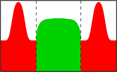
Figure 2: An example of stickiness (the red is the prescribed set, the green is the $s$-minimizer).

Figure 3: Another example of stickiness (the red is the prescribed set, the green is the $s$-minimizer).

Recently, in [2019arXiv190405393D], it was discovered that the boundary discontinuity pointed out in (11) is indeed a “generic” phenomenon at least in the plane: namely if a given graphical external datum produces a continuous minimizer, then an arbitrarily small perturbation of it will produce a minimizer exhibiting the boundary discontinuity.

Interestingly, one of the main ingredients in the proof of the genericity of the boundary discontinuity in [2019arXiv190405393D] consists in an “enhanced boundary regularity”: namely, nonlocal minimal surfaces in the plane with a graphical structure that are continuous at the boundary are automatically $C^{1,\frac{1+\sigma}{2}}$ at the boundary (that is, boundary continuity implies boundary differentiability).

A byproduct of this construction, taking into account also the boundary properties obtained in [MR3532394], is also that nonlocal minimal surfaces with a graphical structure in the plane exhibit a “butterfly effect” for their boundary derivatives: namely, while a nonlocal minimal graph that is continuous at the boundary has also a finite derivative there, an arbitrarily small perturbation of the exterior graph will produce not only a jump at the boundary but also an infinite boundary derivative (that is, the boundary derivative switches from a finite, possibly zero, value to infinity only due to an arbitrarily small perturbation of the datum). We refer to [2019arXiv191205794D] for a survey about this type of phenomena.

It is worth recalling that the boundary discontinuity of nonlocal minimal surfaces is not only a special feature of the nonlocal world, when compared to the case of classical minimal surfaces, but also a special feature of the nonlinear equation of nonlocal mean curvature type, when compared to the case of linear fractional equations: indeed, as detailed in [MR3168912], solutions of linear equations of the type $(-\Delta)^{s}u=f$ in a domain $\Omega$ with an external datum are typically Hölder continuous up to the boundary of $\Omega$, and no better than this (instead, nonlocal minimal surfaces are typically discontinuous at the boundary, but when they are continuous they are also differentiable).

Though this discrepancy between nonlocal minimal surfaces and solutions of linear equations seems a bit surprising at a first glance, a possible explanation for it lies in the “accuracy” of the approximation that a linear equation can offer to an equation of geometric type, such as the one related to the nonlocal mean curvature. Namely, linear equations end up being a good approximation of the geometric equation with respect to the normal of the surface itself: hence, when the surface is “almost horizontal” the graphical structure of the geometric equation is well shadowed by its linear counterpart, but when the surface is “almost vertical” the linear counterpart of the geometric equation should take into account not the graph of the original surface but its “inverse” (i.e., the graph describing the surface in the horizontal, rather than vertical, direction).

We also refer to [2019arXiv190701498D] for a first analysis of the stickiness phenomenon in dimension $3$.

Many examples of nonlocal minimal surfaces exhibiting the stickiness phenomenon are studied in detail in [MR3926519], also with respect to a suitable parameter measuring the weighted measure of the datum at infinity.

In addition, very accurate and fascinating numerical simulations on the stickiness phenomenon of nonlocal minimal surfaces have been recently performed in [MR3982031].

We also remark that nonlocal minimal surfaces with a graphical structure enjoy special regularity properties: for instance they are smooth inside their domain of minimization, as established in [MR3934589].

4 Growth and Bernšteĭn properties of minimal graphs

A classical question, dating back to [zbMATH02583554] is whether or not minimizers of a given geometric problem which have a global graphical structure are necessarily hyperplanes. If this feature holds, we say that the problem enjoys the “Bernšteĭn property”.

This question is also related with the growth of these minimal graphs at infinity. We now discuss and compare the classical and the nonlocal worlds with respect to these features.

4.1 Growth and Bernšteĭn properties of classical minimal graphs

The Bernšteĭn problem for classical minimal surfaces asks whether or not solutions of

$${\rm div}\left(\frac{\nabla u}{\sqrt{1+|\nabla u|^{2}}}\right)=0\;\;{\mbox{ in }}{\mathbb{R}}^{n}$$

are necessarily affine functions.

When $n=2$, a positive answer to this question was provided in [zbMATH02583554]. The development of the theory related to the classical Bernšteĭn problem is closely linked to the regularity theory of classical minimal surfaces, since, as proved in [MR178385], the falsity of the Bernšteĭn property in ${\mathbb{R}}^{n}$ would imply the existence of a singular minimal surface in ${\mathbb{R}}^{n}$.

In light of this connection, the Bernšteĭn property for classical minimal surfaces was established in [MR178385] for $n=3$, in [MR200816] for $n=4$, and in [MR233295] up to $n=7$ (compare with the references in Section 2.1). A counterexample when $n=8$ was then provided in [MR250205], by constructing an eight-dimensional graph in ${\mathbb{R}}^{9}$ which has vanishing mean curvature without being affine.

As a counterpart of this kind of problems, a precise growth analysis of classical minimal surfaces with graphical structure has been obtained in [MR157096] when $n=2$ and in [MR248647] for all dimensions (see also [MR296832, MR308945, MR412605, MR843597, MR2796515] for related results).

More precisely, if $u$ is a solution of

$${\rm div}\left(\frac{\nabla u}{\sqrt{1+|\nabla u|^{2}}}\right)=0\;\;{\mbox{ in }}B_{R}\subset{\mathbb{R}}^{n},$$

then

$$\sup_{B_{R}}|\nabla u|\leqslant\exp\left[C\,\left(1+\frac{\displaystyle\sup_{B_{2R}}u-u(0)}{R}\right)\right],$$ (12)

for some $C>0$ depending only on $n$. Interestingly, this exponential type of gradient estimate is optimal, as demonstrated in [MR157096].

4.2 Growth and Bernšteĭn properties of nonlocal minimal graphs

The Bernšteĭn properties of nonlocal minimal graphs have been investigated in [MR3680376, 2017arXiv170605701F]. In particular, it is proved in these works that the falsity of the nonlocal Bernšteĭn property in ${\mathbb{R}}^{n}$ would imply the existence of a singular nonlocal minimal surface in ${\mathbb{R}}^{n}$, thus providing a perfect counterpart of [MR178385] to the nonlocal setting.

Combining this with the regularity results for nonlocal minimal surfaces in [MR3090533] and [MR3107529], one obtains that the Bernšteĭn property holds true for solutions $u:{\mathbb{R}}^{n}\to{\mathbb{R}}$ of the $\sigma$-mean curvature equation in (5) provided that either $n\in\{1,2\}$, or $n\leqslant 7$ and $\sigma$ is sufficiently close to $1$.

It is an open problem to prove or disprove the Bernšteĭn property for nonlocal minimal graphs $u:{\mathbb{R}}^{n}\to{\mathbb{R}}$ in the general case when $n>2$ and $\sigma\in(0,1)$ (the analysis on symmetric cones performed in [MR3798717] might suggest that new phenomena could arise in dimension $7$).

Concerning the growth of nonlocal minimal surfaces, it has been established in [MR3934589] that if $u:B_{2R}\subset{\mathbb{R}}^{n}\to{\mathbb{R}}$ is a solution of the $\sigma$-mean curvature equation in $B_{2R}$, then

$$\sup_{B_{R}}|\nabla u|\leqslant C\,\left(1+\frac{\displaystyle\sup_{B_{R}}u-\displaystyle\inf_{B_{R}}u}{R}\right)^{n+1+\sigma},$$ (13)

for a suitable constant $C>0$, depending only on $n$ and $\sigma$.

On the one hand, comparing (12) and (13), we observe that the nonlocal world offers us a wealth of surprises: first of all, the estimate in (13) is of polynomial type, rather than of exponential type, as it was the bound in (12). Roughly speaking, this is due to the fact that two different and sufficiently close“ends” of a nonlocal minimal surface repel each other (compare the discussion about the nonlocal catenoid on page 1). Moreover, the right hand side of (13) presents the oscillation of the solution in the same ball $B_{R}$, while (12) needed to extend the right hand side to a larger ball such as $B_{2R}$.

On the other hand, the nonlocal world maintains its own special difficulties: for instance, differently from the classical case, it is an open problem to determine whether the estimate in (13) is optimal.

See Table 1 for a sketchy description of some similarities and differences between classical and nonlocal minimal surfaces.

	classical minimal surfaces	nonlocal minimal surfaces
interior regularity	up to $n=7$ (optimal)	known when $n=2$, and up to $n=7$ if $\sigma$ is large enough (optimality unknown, no singular example available)
boundary regularity	yes for convex (or mean convex) domains	boundary discontinuity (but enhanced differentiable regularity if continuous)
Bernšteĭn property for $u:{\mathbb{R}}^{n}\to{\mathbb{R}}$	up to $n=7$ (optimal)	known when $n=2$, and up to $n=7$ if $\sigma$ is large enough (optimality unknown, no counterexample available)
gradient growth at infinity	exponential (optimal)	polynomial (optimality unknown)

Table 1: Classical versus nonlocal minimal surfaces

5 Phase coexistence models

A physical situation in which minimal interfaces naturally arise occurs in the mathematical description of phase coexistence (or phase transition). In the classical setting, the ansatz is that the short range particle interaction produces a surface tension that leads, on a large scale, to interfaces of minimal area. A modern variation of this model takes into account long-range particle interactions, and we describe here in which sense this model is related to the theory of (non)local minimal surfaces.

5.1 Classical phase coexistence models

One of the most popular phase coexistence models is the one producing the so-called Allen-Cahn equation

$$-\Delta u=u-u^{3}.$$ (14)

Equation (14) has a variational structure, corresponding to critical points of an energy functional of the type

$${\mathcal{F}}(u;\Omega)={\mathcal{F}}(u):=\int_{\Omega}|\nabla u(x)|^{2}+W(u(x))\,dx,$$ (15)

where $W$ is a “double-well” potential attaining its minima at the “pure phases” $-1$ and $+1$.

A classical link between the functional in (15) and the perimeter can be expressed in terms of $\Gamma$-convergence, as stated in [MR445362]. More precisely, given a smooth domain $\Omega\subset{\mathbb{R}}^{n}$ and $\varepsilon>0$, one can consider the rescaled functional

$${\mathcal{F}}_{\varepsilon}(u;\Omega)={\mathcal{F}}_{\varepsilon}(u):=\int_{\Omega}\varepsilon\,|\nabla u(x)|^{2}+\frac{1}{\varepsilon}\,W(u(x))\,dx.$$ (16)

Interestingly, the functional ${\mathcal{F}}_{\varepsilon}$ in (16) inherits the minimization properties of the functional ${\mathcal{F}}$ in (15) after a dilation: for instance, if $u$ is a minimizer for ${\mathcal{F}}$ in every ball, then

$$u_{\varepsilon}(x):=u\left(\frac{x}{\varepsilon}\right)$$ (17)

is a minimizer for ${\mathcal{F}}_{\varepsilon}$ in every ball. Moreover, it holds that:

• for any $u_{\varepsilon}:{\mathbb{R}}^{n}\to[-1,1]$ converging to $u$ in $L^{1}_{\rm loc}({\mathbb{R}}^{n})$, we have that

  $$\liminf_{\varepsilon\searrow 0}{\mathcal{F}}_{\varepsilon}(u_{\varepsilon})\geqslant\mathcal{F}_{0}(u),$$ (18)

• given $u:{\mathbb{R}}^{n}\to[-1,1]$, there exists $u_{\varepsilon}:{\mathbb{R}}^{n}\to[-1,1]$converging to $u$ in $L^{1}_{\rm loc}({\mathbb{R}}^{n})$, such that

  $$\limsup_{\varepsilon\searrow 0}{\mathcal{F}}_{\varepsilon}(u_{\varepsilon})\leqslant\mathcal{F}_{0}(u),$$ (19)

where, for a suitable $c>0$,

$${\mathcal{F}}_{0}(u;\Omega)=\mathcal{F}_{0}(u):=\begin{cases}c\,{\rm Per}(E,\Omega)&\begin{matrix}{\mbox{if $u=\Xi_{E}$}}\\ {\mbox{for some set~{}$E$,}}\end{matrix}\\ \\ +\infty&{\mbox{otherwise.}}\end{cases}$$ (20)

This type of “functional convergence” has also a “geometric counterpart”, given by the locally uniform convergence of levels sets, as established in [MR1310848]. More precisely, if $u$ is a minimizer for ${\mathcal{F}}$ in every ball and $u_{\varepsilon}$ is as in (17), then $u_{\varepsilon}$ converges, up to subsequences, in $L^{1}_{\rm loc}({\mathbb{R}}^{n})$ to some $u=\Xi_{E}$, with $E$ minimizing the perimeter, and the level sets of $u_{\varepsilon}$ approach $\partial E$ locally uniformly, that is, given any $\vartheta\in(0,1)$, any $R>0$ and any $\delta>0$ there exists $\varepsilon_{0}\in(0,1)$ such that, if $\varepsilon\in(0,\varepsilon_{0})$, we have that

$$\big{\{}|u_{\varepsilon}|<1-\theta\big{\}}\cap B_{R}\subseteq\bigcup_{p\in\partial E}B_{\delta}(p).$$ (21)

The level set convergence in (21) relies on suitable “energy and density estimates” stating that the energy behaves as an “interface” and, in a neighborhood of the interface, both the phases have positive densities. More precisely, if $R\geqslant 1$ and $u$ is a minimizer of ${\mathcal{F}}$ in $B_{R+1}$, then

$${\mathcal{F}}_{B_{R}}(u)\leqslant CR^{n-1},$$ (22)

for some $C>0$, and, for every $\vartheta_{1},\vartheta_{2}\in(0,1)$, if $|u(0)|\leqslant\vartheta_{1}$ then

$$\begin{split}&\{u\geqslant\vartheta_{2}\}\cap B_{R}\geqslant cR^{n}\\ {\mbox{and}}\qquad&\{u\leqslant-\vartheta_{2}\}\cap B_{R}\geqslant cR^{n}.\end{split}$$ (23)

5.2 Long-range phase coexistence models

In the recent literature a number of models have been introduced in order to study phase coexistence driven by long-range particle interactions, see e.g. [MR1612250, MR2223366].

We describe here a simple model of this kind, comparing the results obtained in this situation with the classical ones presented in Section 5.1.

We focus on a nonlocal version of the Allen-Cahn equation (14) given by

$$(-\Delta)^{s}u=u-u^{3},$$ (24)

with $s\in(0,1)$. Equation (24) has a variational structure, corresponding to critical points of an energy functional of the type

$$\begin{split}&{\mathcal{E}}(u;\Omega)={\mathcal{E}}(u):=\int_{Q_{\Omega}}\frac{|u(x)-u(y)|^{2}}{|x-y|^{n+2s}}\,dx\,dy\\ &\qquad\qquad+\int_{\Omega}W(u(x))\,dx,\end{split}$$ (25)

where $W$ is a “double-well” potential attaining its minima at the “pure phases” $-1$ and $+1$, and $Q_{\Omega}$ is the cross-type domain given by

$$(\Omega\times\Omega)\cup(\Omega\times\Omega^{c})\cup(\Omega^{c}\times\Omega).$$

The rationale behind this choice of $Q_{\Omega}$ is to collect all the couples of points in which at least one of the two lies in $\Omega$, so to comprise all the point interactions that involve $\Omega$ (a similar choice was performed in the geometric problem (4)).

The $\Gamma$-convergence theory for the functional in (25) has been established in [MR2948285]. For this, one needs to introduce a family of rescaled functional with different scaling properties depending on the fractional parameter $s$. More precisely, it is convenient to define

$$\begin{split}&{\mathcal{E}}_{\varepsilon}(u;\Omega)={\mathcal{E}}_{\varepsilon}(u):=a_{\varepsilon}\,\int_{Q_{\Omega}}\frac{|u(x)-u(y)|^{2}}{|x-y|^{n+2s}}\,dx\,dy\\ &\qquad\qquad+b_{\varepsilon}\,\int_{\Omega}W(u(x))\,dx,\end{split}$$ (26)

where

$$a_{\varepsilon}:=\begin{cases}\varepsilon^{2s-1}&{\mbox{ if }}s\in(1/2,\,1),\\ |\log\varepsilon|^{-1}&{\mbox{ if }}s=1/2,\\ 1&{\mbox{ if }}s\in(0,\,1/2),\end{cases}$$

and

$$b_{\varepsilon}:=\varepsilon^{-2s}a_{\varepsilon}=\begin{cases}\varepsilon^{-1}&{\mbox{ if }}s\in(1/2,\,1),\\ \varepsilon^{-1}|\log\varepsilon|^{-1}&{\mbox{ if }}s=1/2,\\ \varepsilon^{-2s}&{\mbox{ if }}s\in(0,\,1/2).\end{cases}$$

The coefficients $a_{\varepsilon}$ and $b_{\varepsilon}$ are tuned with respect to the energy of a one-dimensional layer joining $-1$ and $+1$ and, in this way, the functional ${\mathcal{E}}_{\varepsilon}$ in (26) satisfies some interesting $\Gamma$-convergence properties. Remarkably, these properties are very sensitive to the fractional parameter $s$: indeed, when $s<1/2$ the $\Gamma$-convergence theory obtains the $\sigma$-perimeter introduced in (4), with $\sigma:=2s$, but when $s\geqslant 1/2$, the nonlocal character of the problem is lost in the limit and the $\Gamma$-convergence theory boils down to the classical one in (18), (19) and (20).

More precisely, one can define

$${\mathcal{E}}_{0}(u;\Omega)=\mathcal{E}_{0}(u):=\begin{cases}c\,{\rm Per}(E,\Omega)&\begin{matrix}{\mbox{if $s\in[1/2,1)$}}\\ {\mbox{and $u=\Xi_{E}$}}\\ {\mbox{for some set~{}$E$,}}\end{matrix}\\ \\ c\,{\rm Per}_{2s}(E,\Omega)&\begin{matrix}{\mbox{if $s\in(0,1/2)$}}\\ {\mbox{and $u=\Xi_{E}$}}\\ {\mbox{for some set~{}$E$,}}\end{matrix}\\ \\ +\infty&{\mbox{otherwise.}}\end{cases}$$

In this sense, the functional ${\mathcal{E}}_{0}$ is the “natural replacement” of the one in (20) to deal with the $\Gamma$-convergence of nonlocal phase transitions, in the sense that the statements in (18), (19) and (20) hold true in this case with ${\mathcal{F}}_{\varepsilon}$ replaced by ${\mathcal{E}}_{\varepsilon}$ and ${\mathcal{F}}_{0}$ replaced by ${\mathcal{E}}_{0}$.

For additional discussions of nonlocal $\Gamma$-convergence results, see [2020arXiv200101475D].

The convergence of level sets in (21) has also a perfect counterpart for the minimizers of ${\mathcal{E}}$, as established in [MR3133422]. These results also rely on suitable density estimates which guarantee that (23) also holds true for minimizers of ${\mathcal{E}}$.

However, in this case, an energy estimate as in (22) exhibits a significant difference, depending on the fractional exponent $s$. Indeed, in this framework, we have that if $R\geqslant 2$ and $u$ is a minimizer of ${\mathcal{E}}$ in $B_{R+1}$, then

$${\mathcal{E}}_{B_{R}}(u)\leqslant\begin{cases}CR^{n-1}&{\mbox{ if }}s\in(1/2,\,1),\\ CR\,\log R&{\mbox{ if }}s=1/2,\\ CR^{n-2s}&{\mbox{ if }}s\in(0,\,1/2),\end{cases}$$ (27)

for some $C>0$.

In spite of its quantitative difference with (22), the estimate in (27) is sufficient to determine that the interface contribution is “negligible” with respect to the Lebesgue measure of large balls. Moreover, such an estimate is in agreement with the energy of one-dimensional layers.

We refer to Table 2 for a schematic representation of similarities and differences of classical and nonlocal phase transitions in terms of $\Gamma$-limits and density estimates.

In addition, long- phase transition models and nonlocal minimal surfaces have close connections with spin models and discrete systems, see [MR1372427, MR1453735, MR1794850, MR2219278, MR2608835, MR3017265, MR3472011] and the references therein. In particular, in [MR3652519] the reciprocal approximation of ground states for long-range Ising models and nonlocal minimal surfaces has been established and the relation between these two problems has been investigated in detail.

	phase transitions $s\in(0,1/2)$	phase transitions $s=1/2$	phase transitions $s\in(1/2,1]$
$\Gamma$-limit	nonlocal perimeter	classical perimeter	classical perimeter
energy estimates	$R^{n-2s}$	$R\,\log R$	$R^{n-1}$

Table 2: Classical versus nonlocal phase transitions

6 Geometric flows

Another classical topic in geometric analysis consists in the study of evolution equations describing the motion of set boundaries. In this framework, at any time $t$, one prescribes the speed $V$ of a hypersurface $\partial E_{t}$ in the direction of the outer normal to $E_{t}$.

In this section, in light of the setting in (5), we will describe analogies and differences between the classical and the nonlocal mean curvature flows.

6.1 Mean curvature flow

One of the widest problem in geometric analysis focuses on the case in which the normal velocity $V$ of the flow is taken to be the classical mean curvature. This flow decreases the classical perimeter and has a number of remarkable properties. A convenient description of the mean curvature flow can be given in terms of viscosity solutions, using a level set approach, see [MR1100206]. See also [MR1100211, MR1360824] for related viscosity methods. If the initial hypersurface satisfies a Lipschitz condition, then the mean curvature flow possesses a short time existence theory, see [MR1117150]. In general, the flow may develop singularities, and the understanding of the different possible singularities is a very rich and interesting field of investigation in itself, see e.g. [MR485012, MR2024995, MR2815949].

The planar case $n=2$ presents some special feature. In this case, the flow becomes “curve shortening” in the sense that its special characteristic is to decrease the length of a given closed curve as fast as possible. In this setting, it was proved in [MR0906392] that the curve shortening flow makes every smooth closed embedded curves in the plane shrink smoothly to round points (i.e., the curve shrinks becoming “closer and closer to a circle”). More precisely: on the one hand, as shown in [MR0840401], if the initial curve is convex, then the evolving curve remains convex and becomes asymptotically circular as it shrinks; on the other hand, as shown in [MR0906392], if the curve is only embedded, then no singularity develops before the curve becomes convex, then shrinking to a round point.

These results can be also interpreted in light of a “distance comparison property”. Namely, given two points $p$ and $q$ on the evolving surface, one can consider the “extrinsic” distance $d=d(p,q)$, given by the Euclidean distance of $p$ and $q$, and the arc-length “intrinsic” distance $\ell=\ell(p,q)$, that measures the distance of $p$ and $q$ along the curve. For a closed curve of length $L$, one can also define

$$\lambda:=\frac{L}{\pi}\,\sin\frac{\pi\ell}{L}.$$

Then, as proved in [MR1656553], we have that the minimal ratio $\rho:=\min\frac{d}{\lambda}$ is nondecreasing under the curve shortening flow (and, in fact, strictly increasing unless the curve is a circle). In this spirit, the ratio $\rho$ plays the role of an improving isoperimetric quantity which measures the deviation of the evolving curve from a round circle. In particular, if a curve developed a “neckpinch”, it would present two points for which $d=0$ and $\ell>0$, hence $\rho=0$: as a consequence, the monotonicity proved in [MR1656553] immediately implies that planar curves do not develop neckpinches under the curve shortening flow. More generally, the results in [MR1656553] can be seen as a quantitative refinement of those in [MR0840401, MR0906392]. See also [MR0772132] for related results.

In any case, for the mean curvature flow, the formation of neckpinch singularity for the evolving hypersurface can only occur (and it occurs) in dimension $n\geqslant 3$, see [MR1030675, MR3803553].

6.2 Nonlocal mean curvature flow

A natural variant of the flow discussed in Section 6.1 consists in taking as normal velocity the nonlocal mean curvature of the evolving set, as given in (5). The main feature of this evolution problem is that it decreases the nonlocal perimeter defined in (4).

This evolution problem emerged in [MR2487027, MR2564467]. A detailed viscosity solution theory for the nonlocal mean curvature flow has been presented in [MR3156889], see also [MR3401008] for more general results.

In the viscosity setting, given an initial set $E\subset{\mathbb{R}}^{n}$, the evolution of $E$ is described by level sets of a function $u_{E}=u_{E}(x,t)$ which solves a parabolic problem driven by the nonlocal mean curvature. More precisely, the evolution of $E$ is trapped between an outer and an inner flows defined by

$$E^{+}(t):=\{x\in{\mathbb{R}}^{n}{\mbox{ s.t. }}u_{E}(x,t)\geqslant 0\}$$

and $$E^{-}(t):=\{x\in{\mathbb{R}}^{n}{\mbox{ s.t. }}u_{E}(x,t)>0\}.$$

The ideal case would be the one in which these two flows coincide “up to a smooth manifold” which describes the evolving surface, i.e. the case in which

$$\begin{split}\Sigma_{E}(t)\,&:=\,E^{+}(t)\setminus E^{-}(t)\\ &=\,\{x\in{\mathbb{R}}^{n}{\mbox{ s.t. }}u_{E}(x,t)=0\}\end{split}$$ (28)

is a nice hypersurface, but, in general, such a property is not warranted by the notion of viscosity solutions.

A short-time existence theory of smooth solutions of the nonlocal mean curvature flow has been recently established in [2019arXiv190610990J] under the assumption that the initial hypersurface is of class $C^{1,1}$. As far as we know, it is still an open problem to determine whether the nonlocal mean curvature flow possesses a short-time existence theory of smooth solutions for Lipschitz initial data (this would provide a complete counterpart of the classical results in [MR1117150]).

It is certainly interesting to detect suitable information that are preserved by the nonlocal mean curvature flow. For instance: the fact that the nonlocal mean curvature flow preserves the positivity of the nonlocal mean curvature itself has been established in [MR3951024], and the preservation of convexity has been proved in [MR3713894].

An important difference between the classical and the nonlocal mean curvature flows consists in the “fattening phenomena” of viscosity solutions, in which the set in (28) may develop a nonempty interior (thus failing to be a nice hypersurface), as investigated in [MR4000255]. For instance, one can consider the case in which the initial set is the “cross in the plane” given by

$$E=\{(x,y)\in{\mathbb{R}}^{2}{\mbox{ s.t. }}|x|>|y|\}.$$ (29)

In this situation, using the notation in (28), one can prove that $\Sigma_{E}(t)$ is nontrivial and immediately develops a positive measure: more precisely, we have that $\Sigma_{E}(t)$ contains the ball $B_{ct^{\frac{1}{1+s}}}$, for some $c>0$.

On the one hand, this result is in agreement with the classical case, since also the classical mean curvature flow develops this kind of situations when starting from the set in (29) (see [MR1100206]).

On the other hand, the fattening phenomena for the nonlocal situation offers a number of surprises with respect to the classical case (see [MR4000255]). First of all, the quantitative properties of the interaction kernels play a decisive role in the development of the fat portions of $\Sigma_{E}(t)$ and in general on the evolution of the set $E$. For instance, if the interaction kernel $\frac{1}{|x-y|^{n+\sigma}}$ in (1) is replaced by a different kernel that is smooth and compactly supported, then the nonlocal mean curvature flow of the cross $E$ in (29) does not develop any fattening and, more precisely, the evolution of $E$ would be $E$ itself (in a sense, we switch from a fattening situation, produced by singular kernels with slow decay, to a “pinning effect” produced by smooth and compactly supported kernels).

Furthermore, there are cases in which the fattening phenomena are different according to the type of local or nonlocal mean curvature flow that we consider (see [MR1100206]). For instance, if the initial set is made by two tangent balls in the plane such as

$$E:=B_{1}(-1,0)\cup B_{1}(1,0),$$ (30)

then, for the nonlocal mean curvature flow, using the notation in (28), we have that $\Sigma_{E}(t)$ has empty interior for all $t>0$. This situation is different with respect to the classical mean curvature flow, which immediately develops fattening (see [MR1298266]).

The nonlocal mean curvature flow (and its many variants) are a great source of intriguing questions and mathematical adventures. Among the interesting questions remained open, we mention that it is not known whether the nonlocal mean curvature flow possesses a nonlocal version of the monotonicity formula in [MR1656553], or what a natural replacement of it could be. This question is also related to a deeper understanding of the singularities of the nonlocal mean curvature flow.