Temporal Network Representation Learning via Historical Neighborhoods Aggregation

Abstract

Network embedding is an effective method to learn low-dimensional representations of nodes, which can be applied to various real-life applications such as visualization, node classification, and link prediction. Although significant progress has been made on this problem in recent years, several important challenges remain, such as how to properly capture temporal information in evolving networks. In practice, most networks are continually evolving. Some networks only add new edges or nodes such as authorship networks, while others support removal of nodes or edges such as internet data routing. If patterns exist in the changes of the network structure, we can better understand the relationships between nodes and the evolution of the network, which can be further leveraged to learn node representations with more meaningful information. In this paper, we propose the Embedding via Historical Neighborhoods Aggregation (EHNA) algorithm. More specifically, we first propose a temporal random walk that can identify relevant nodes in historical neighborhoods which have impact on edge formations. Then we apply a deep learning model which uses a custom attention mechanism to induce node embeddings that directly capture temporal information in the underlying feature representation. We perform extensive experiments on a range of real-world datasets, and the results demonstrate the effectiveness of our new approach in the network reconstruction task and the link prediction task.

I introduction

Network embedding has become a valuable tool for solving a wide variety of network algorithmic problems in recent years. The key idea is to learn low-dimensional representations for nodes in a network. It has been applied in various applications, such as link prediction [1], network reconstruction [2], node classification [3] and visualization [4]. Existing studies [1, 2, 3, 4] generally learn low-dimensional representations of nodes over a static network structure by making use of contextual information such as graph proximity.

However, many real-world networks, such as co-author networks and social networks, have a wealth of temporal information (e.g., when edges were formed). Such temporal information provides important insights into the dynamics of networks, and can be combined with contextual information in order to learn more effective and meaningful representations of nodes. Moreover, many application domains are heavily reliant on temporal graphs, such as instant messaging networks and financial transaction graphs, where timing information is critical. The temporal/dynamic nature of social networks has attracted considerable research attention due to its importance in many problems, including dynamic personalized pagerank [5], advertisement recommendation [6] and temporal influence maximization [7], to name a few. Despite the clear value of such information, temporal network embeddings are rarely applied to solve many other important tasks such as network reconstruction and link prediction [8, 9].

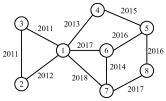
Figure 1: An example of a co-author temporal network. Each edge is annotated with a timestamp denoting when the edge was created.

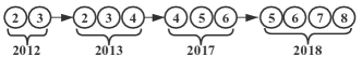
Figure 2: The evolution of a set of nodes that are contextually and temporally related to node 1.

Incorporating temporal information into network embeddings can improve the effectiveness in capturing relationships between nodes which can produce performance improvements in downstream tasks. To better understand the relationships between nodes with temporal information in a network, consider Figure 1 which is an ego co-author network for a node (1). Each node is an author, and edges represent collaborations denoted with timestamps. Without temporal knowledge, the relationships between nodes 2, 3, 4, 6 and 7 are indistinguishable since they are all connected to node 1. However, when viewed from the temporal perspective, node 1 once was ‘close’ to nodes 2 and 3 but now is ‘closer’ to nodes 4, 6 and 7 as node 1 has more recent and frequent collaborations with the latter nodes. Furthermore, in the static case, nodes 2 and 3 appear to be ‘closer’ to node 1 than node 5, since nodes 2 and 3 are direct neighbors of node 1, whereas node 5 is not directly connected to node 1. A temporal interpretation suggests that node 5 is also important to 1 because node 5 could be enabling collaborations between nodes 1 6, and 7. Thus, with temporal information, new interpretations of the ‘closeness’ of relationships between node 1 and other nodes and how these relationships evolve are now possible.

To further develop this intuition, consider the following concrete example. Suppose node 1 began publishing as a Ph.D. student. Thus, papers produced during their candidature were co-authored with a supervisor (node 3) and one of the supervisor’s collaborators (node 2). After graduation, the student (node 1) became a research scientist in a new organization. As a result, a new collaboration with a senior supervisor (node 4) is formed. Node 1 was introduced to node 5 through collaborations between the senior supervisor (node 4) and node 5, and later began working with node 6 after the relationship with node 5 was formed. Similarly, after a collaboration between node 1 and node 6, node 1 met node 7 because of the relationships between node 5 and node 8, node 8 and node 7, and node 6 and node 7. Hence, as shown in Figure 2, both the formation of the relationships between node 1 and other nodes and the levels of closeness of such relationships evolve as new connections are made between node 1 and related collaborators.

Thus, the formation of each edge $(x,y)$ changes not only the relationship between $x$ and $y$ but also relationships between nodes in the surrounding neighborhood. Capturing how and why a network evolves (through edge formations) can produce better signals in learned models. Recent studies capture the signal by periodically probing a network to learn more meaningful embeddings. These methods model changes in the network by segmenting updates into fixed time windows, and then learn an embedding for each network snapshot [10, 11]. The embeddings of previous snapshots can be used to infer or indicate various patterns as the graph changes between snapshots. In particular, CTDNE [12] leveraged temporal information to sample time-constrained random walks and trained a skip-gram model such that nodes co-occurring in these random walks produce similar embeddings. Inspired by the Hawkes process [13] which shows that the occurrence of current events are influenced by the historical events, HTNE [14] leveraged prior neighbor formation to predict future neighbor formations. In this paper, we show how to more effectively embed fine-grained temporal information in all learned feature representations that are directly influenced by historical changes in a network.

How to effectively analyze edge formations is a challenging problem, which requires: (1) identifying relevant nodes (not limited to direct neighbors) which may impact edge formations; (2) differentiating the impact of relevant nodes on edge formations; (3) effectively aggregating useful information from relevant nodes given a large number of useful but noisy signals from the graph data.

To mitigate these issues, we propose a deep learning method, which we refer to as Embedding via Historical Neighborhoods Aggregation (EHNA), to capture node evolution by probing the information/factors influencing temporal behavior (i.e., edge formations between nodes). To analyze the formation of each edge $(x,y)$, we apply the the following techniques. First, a temporal random walk is used to dynamically identify relevant nodes from historical neighborhoods that may influence new edge formations. Specifically, our temporal random walk algorithm models the relevance of nodes using a configurable time decay, where nodes with high contextual and temporal relevance are visited with higher probabilities. Our temporal random walk algorithm can preserve the breadth-first search (BFS) and depth-first search (DFS) characteristics of traditional solutions, which can then be further exploited to provide both micro and macro level views of neighborhood structure for the targeted application. Second, we also introduce a two-level (node level and walk level) aggregation strategy combined with stacked LSTMs to effectively extract features from nodes related to chronological events (when edges are formed). Third, we propose a temporal attention mechanism to improve the quality of the temporal feature representations being learned based on both contextual and temporal relevance of the nodes.

Our main contributions to solve the problem of temporal network representation learning are:

• We leverage temporal information to analyze edge formations such that the learned embeddings can preserve both structural network information (e.g., the first and second order proximity) as well as network evolution.

• We present a temporal random walk algorithm which dynamically captures node relationships from historical graph neighborhoods.

• We deploy our temporal random walk algorithm in a stacked LSTM architecture that is combined with a two-level temporal attention and aggregation strategy developed specifically for graph data, and describe how to directly tune the temporal effects captured in feature embeddings learned by the model.

• We show how to effectively aggregate the resulting temporal node features into a fixed-sized readout layer (feature embedding), which can be directly applied to several important graph problems such as link prediction.

• We validate the effectiveness of our approach using four real-world datasets for the network reconstruction and link prediction tasks.

Organization of this paper. Related work is surveyed in Section II and our problem formulation is presented in Section III. Next, we describe the problem solution in Section IV. We empirically validate our new approach in Section V, and conclude in Section VI.

II Related Work

Static network embedding. Inspired by classic techniques for dimensionality reduction [15] and multi-dimensional scaling [16], early methods [15, 17, 18, 19] focused on matrix-factorization to learn graph embeddings. In these approaches, node embeddings were learned using a deterministic measure of graph proximity which can be approximated by computing the dot product between learned embedding vectors. Methods such as DeepWalk [3] and Node2Vec [1] employed a more flexible, stochastic measure of graph proximity to learn node embeddings such that nodes co-occurring in short random walks over a graph produce similar embeddings. A more contemporaneous method, Line [4], combined two objectives that optimize ‘first-order’ and ‘second-order’ graph proximity, respectively. sdne [2] extended this idea of Line to a deep learning framework [20] which simultaneously optimizes these two objectives. A series of methods [21, 22, 23] followed which further improved the effectiveness and/or scalability of this approach.

More recently, Graph Convolutional Networks (gcn) were proposed and are often more effective than the aforementioned methods for many common applications, albeit more computationally demanding. These models can directly incorporate raw node features/attributes and inductive learning into nodes absent during the initial training process. gcn methods generate embeddings for nodes by aggregating information from neighborhoods. This aggregation process is called a ‘convolution’ as it represents a node as a function of the surrounding neighborhood, in a manner similar to center-surrounded convolutional kernels commonly used in computer vision [24, 25]. To apply convolutional operations on graph data, Bruna et al. [26] computed the point-wise product of a graph spectrum in order to induce convolutional kernels. To simplify the spectral method, Kips et al. [24] applied a Fourier transform to graph spectral data to obtain filters which can be used to directly perform convolutional operations on graph data. GraphSAGE [25] proposed a general learning framework which allows more flexible choices of aggregation functions and node combinations such that it gave significant gains in some downstream tasks. There are also several related gcn based methods [24, 27, 28, 29, 30, 31, 32] which differ primarily in how the aggregation step is performed. Despite significant prior work, all of these methods focused on preserving static network information.

Dynamic network embedding. Several recent methods have also been proposed to model the dynamic nature of networks. Zhu et al. [11] proposed a matrix factorization-based algorithm for dynamic network embedding. Yang et al. [10] explored the evolutionary patterns of triads to capture structural information to learn latent representation vectors for vertices at different timesteps. These methods [11, 10] modeled the dynamics by segmenting the timelines into fixed windows and the resulting embeddings only represent individual snapshots of a network. Embeddings of previous snapshots can then be used to infer or indicate various patterns of a graph as it changes between snapshots. ctdne [12] extended the well-known Node2Vec [1] embedding approach to temporal data by imposing a temporal ordering restriction on the random walk process such that random walks are one-directional (increasing in time). The skip-gram model adopted by ctdne [12] attempts to induce co-occurring nodes in a constrained random walk to produce similar embeddings. However, these methods [10, 11, 12] only leverage temporal information at a coarse level and thus may not fully capture the evolution of a temporal network. Inspired by the conditional intensity function of the Hawkes process [13] which showed that the occurrence of a current event is influenced by prior events, htne [14] modeled neighborhood formation sequences such that the current neighbor formation is influenced with a higher “intensity” by more recent historical neighbor formations. However, edge formations are not just influenced by directly connected neighbors, and the process described is not able to directly benefit from the influence of surrounding nodes unless direct connections are formed.

III Problem Formulation

In this section, we proceed to formulate our problem.

Definition 1

(Temporal Network). A temporal network is a network $\mathcal{G}=(\mathcal{V},\mathcal{E})$ where $\mathcal{V}$ denotes the set of nodes, $\mathcal{E}$ denotes the set of edges and each edge $(x,y)\in\mathcal{V}$ is annotated with a timestamp $t_{(x,y)}$, describing when edge $(x,y)$ was formed.

Given a temporal network, the evolution of new connections to node $x$ are influenced by nodes close to $x$. Specifically, the formation of each edge $(x,y)$ is influenced by relevant nodes which have direct or indirect historical interactions with $x$ or $y$ before time $t_{(x,y)}$ in a neighborhood.

Definition 2

(Relevant Node). For each edge $(x,y)$, a node $w$ is relevant to the formation of $(x,y)$ if and only if $w$ can reach $x$ or $y$ through (in)direct historical interactions (e.g., historical edges) $I=\{a_{1}-a_{2}-a_{3}-\cdots-a_{i}\}$ such that $\forall(a_{j},a_{j+1})\in I,t_{(a_{j},a_{j+1})}\leq t_{(a_{j+1},a_{j+2})}$, where $a_{1}=w$, $a_{i}=x$ or $y$.

In our problem, we will use temporal random walks to identify relevant nodes. In particular, we aim to capture the network evolution as well as structural information (e.g., the first-order and second-order proximity) in the learned node embeddings.

Definition 3

(First-order Proximity [4]). The first-order proximity in a network is the local pairwise proximity between two nodes. For each pair of nodes linked by an edge $(x,y)$, the weight on that edge, $w_{xy}$, indicates the first-order proximity between $x$ and $y$. $w_{xy}>0$ in a weighted graph and $w_{xy}=1$ in an unweighted graph. If no edge is observed between $x$ and $y$, their first-order proximity is 0.

Definition 4

(Second-order Proximity [4]). The second-order proximity between a pair of nodes $(x,y)$ in a network is the similarity between their neighborhood network structures. Mathematically, let $p_{u}=(w_{x,1},\ldots,w_{x,|V|})$ denote the first-order proximity of $x$ with all the other vertices, then the second-order proximity between $x$ and $y$ is determined by the similarity between $p_{x}$ and $p_{y}$. If no vertex is linked from/to both $x$ and $y$, the second-order proximity between $x$ and $y$ is 0.

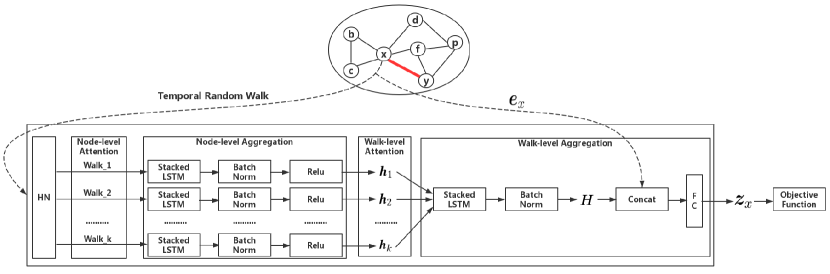
Figure 3: The EHNA Framework.

Problem 1 (Temporal Network Embedding): Given a temporal network $\mathcal{G}=(\mathcal{V},\mathcal{E})$, we aim to learn a mapping function $f:v\rightarrow\bm{e}_{v}\in\mathbb{R}^{d}$ where $v\in\mathcal{V},d\ll|\mathcal{V}|$. The objective function captures:
(1) the Euclidean distance between $\bm{e}_{x}$ and $\bm{e}_{y}$ to be small in the embedding space if $x$ and $y$ share an edge;
(2) the Euclidean distance between $\bm{e}_{x}$ and $\bm{e}_{y}$ to be large if no link is between $x$ and $y$;
(3) $\bm{e}_{x}$ and $\bm{e}_{y}$ in the embedding space preserve the first-order and second-order proximity of $x$ and $y$, and the likelihood of being connected with other nodes in the future.

IV Historical Neighborhood Aggregation (ehna)

Figure 3 provides an overview of our EHNA framework, where HN, Concat and FC stands for the Historical Neighborhood (HN), a concatenation operator and a fully connected layer respectively. The historical neighborhood of node $x$ is a subgraph formed by the nodes and edges traversed by temporal random walks initiated at $x$. Note that the procedure illustrated by this framework is applied to both target nodes of every edge analyzed. We demonstrate the main procedure using only one target node to improve clarity. To analyze the formation of each edge $(x,y)$, we first apply temporal random walks to identify nodes which are relevant to the target node $x$ ($y$). Then we apply a two-level aggregation strategy to extract useful temporal information that might influence future behaviors (e.g, the formation of $(x,y)$) of $x$ ($y$). For the first level aggregation, we apply a node-level temporal attention mechanism to individual nodes occurring in random walks in order to capture node-level temporal and contextual information. During second level aggregation we induce walk-level temporal information in the feature vectors. Next, the aggregated embedding $\bm{z}_{x}\;(\bm{z}_{y})$ of the target node $x$ ($y$) is created by combining the representation $\bm{e}_{x}\;(\bm{e}_{y})$ of $x$ ($y$) with information aggregated from the surrounding neighborhood. Finally, we optimize our objective function using the aggregated embeddings of the target nodes.

In the remainder of this section, we will first introduce the temporal random walk. Then, we explain how to achieve two-level aggregation using our custom attention mechanism, and describe how to optimize $\bm{z}_{x}$ .

IV-A Temporal Random Walk

To analyze the formation of a target edge $(x,y)$, we use a temporal random walk to find relevant nodes (Definition 2) which may have impacted the formation of $(x,y)$. In our temporal random walk algorithm, the transition probability $w^{\mathcal{T}}_{(u,v)}$ of each edge $(u,v)$ is directly associated with two factors, the original weight $w_{(u,v)}$ of $(u,v)$ and the temporal information $t_{(u,v)}$ of $(u,v)$. To make sure that nodes that have more recent (in)direct interactions with $x$ or $y$ are more likely to be visited in the random walks, we use a kernel function $\mathcal{K}$ of $t_{(x,y)}$, $t_{(u,v)}$ and $w_{(u,v)}$ to create $w^{\mathcal{T}}_{(u,v)}$ where $\mathcal{K(\cdot)}$ denotes the time decay effect and can be expressed in the form of an exponential decay function as:

$$\begin{split}w^{\mathcal{T}}_{(u,v)}&=\mathcal{K}(t_{(x,y)},t_{(u,v)},w_{(u,v)})\\ &=w_{(u,v)}\cdot\exp(-(t_{(x,y)}-t_{(u,v)}))\end{split}$$ (1)

In a manner similar to Node2Vec [1], we introduce additional parameters to control the bias of the temporal random walk towards different search traversals – a depth-first search (DFS) or a breadth-first search (BFS). By tuning this parameter, we can ensure that the temporal random walk captures multiple traversal paths (microscopic and macroscopic) of the neighborhood, and the embeddings being learned can emphasize both community and/or highly localized structural roles specific to the target application.

For example, suppose that we require a temporal random walk which identifies the historical neighborhood of $x$ or $y$ to analyze the formation of $(x,y)$. The walk has just traversed edge $(u,v)$ and now resides at node $v$. For each outgoing edge $(v,w)$, we set the unnormalized transition probability to $\pi_{(v,w)}=\beta_{(u,w)}\cdot\mathcal{K}(t_{(x,y)},t_{(v,w)},w_{(v,w)})$ where

$$\beta_{(u,w)}=\left\{\begin{aligned} \frac{1}{p}&\;\;\;if\;d_{uw}=0,\;t_{(u,v)}\geq t_{(v,w)}\\ 1&\;\;\;if\;d_{uw}=1,\;t_{(u,v)}\geq t_{(v,w)}\\ \frac{1}{q}&\;\;\;if\;d_{uw}=2,\;t_{(u,v)}\geq t_{(v,w)}\\ 0&\;\;\;if\;t_{(u,v)}<t_{(v,w)}\end{aligned}\right.$$ (2)

and $d_{uw}$ denotes the shortest path distance between $u$ and $w$. By tuning the parameters $q$ and $p$, the random walk can prefer either a BFS or DFS traversal. More specifically, $d_{uw}$ can only have three possible values in Equation 2: (1) $d_{uw}=0$ refers to traveling from $v$ back to $u$; (2) $d_{uw}=1$ refers to traveling from $v$ to $w$ which is one hop away from $u$; (3) $d_{uw}=2$ refers to traveling from $v$ to $w$ which is two hops away from $u$. Thus, the parameter $p$ controls the likelihood of immediately revisiting a previous node in the walk and the parameter $q$ controls the bias towards BFS or DFS. By combining $\beta$ and the kernel function $\mathcal{K(\cdot)}$ to compute the transition probabilities, we are able to effectively find historical neighborhoods where nodes not only have high affinity with $x$ or $y$ based on the static network structure, but also have high relevance to the formation of $(x,y)$. Moreover, allowing duplicate visits in the temporal random walks can effectively mitigate any potential sparsity issues in the temporal random walk space. Specifying the number of walk steps as a walk length is a standard procedure applied in random walk algorithms, and each random walk will not stop until that number of steps is reached. In our temporal random walk algorithm, we only visit relevant nodes, which are defined using the constraints shown in Definition 2. If backtracking is not allowed and no unvisited neighbor is “relevant”, the temporal random walk will early terminate before the pre-defined number of walk steps can be reached.

IV-B Node-level Attention and Aggregation

Input : Graph $G=(V,E)$, the target edge $(x,y)$ and target node $x$, node embeddings {$\bm{e}_{v},\forall v\in\mathcal{V}$ }, a weight matrix $W$, the number of walks $k$, walk length $\ell$.

Output : Aggregated embedding $\bm{z}_{x}$ of $x$ after aggregation.

1 for  $i=1$ to $k$ do

2       $S_{i}\leftarrow$ nodes in random walk $\textbf{{r}}_{i}$ of length $\ell$ ;

3       Compute $\alpha_{v,x}$ for {$\bm{e}_{v},\forall v\in S_{i}$ } ;

4       $\bm{h}_{\textbf{{r}}_{i}}=\text{Relu}\big{(}\text{BN}\big{(}\text{LSTM}\big{(}\{\alpha_{v,x}\bm{e}_{v},\forall v\in S_{i}\}\big{)}\big{)}\big{)}$ ;

5Compute $\beta_{\textbf{{r}}_{i},x}$ for {$\textbf{{r}}_{i},\forall i\in\{1,2,...,k\}$ } ;

6 $\bm{{H}}\leftarrow\text{BN}$(LSTM({$\beta_{\textbf{{r}}_{i},x}\bm{h}_{\textbf{{r}}_{i}},\forall i\in\{1,2,...,k\}$ })) ;

7 $\bm{z}_{x}\leftarrow W\cdot[\bm{H}||\bm{e}_{x}]$ ;

8 Return $\bm{z}_{x}\leftarrow\bm{z}_{x}/\|\bm{z}_{x}\|_{2}$ ;

Algorithm 1 Forward propagation of the aggregation process

During first level aggregation, we combine information from nodes appearing in the same random walks instead of processing all nodes in a historical neighborhood deterministically. This strategy has two benefits: (1) it reduces the number of nodes being aggregated, while still improving the effectiveness (only the most relevant nodes are covered), and can lead to faster convergence; (2) each random walk can be roughly regarded as a sequence of chronological events (e.g., edge formations) which can be leveraged to capture more meaningful information (i.e., the sequential interactions/relationships between nodes). In a manner commonly used for sequential data in the NLP community, each random walk can be viewed as a ‘sentence’, and a stacked LSTM (multi-layer LSTM) can then be applied as the aggregator. Below is a sketch of the workflow of node-level aggregation:

$$\bm{h}=\text{Relu}\big{(}\text{BN}\big{(}\text{AGGREGATE\big{(}Input\textsubscript{1}\big{)}}\big{)}\big{)}$$

where (1) Input₁ = {$\bm{e}_{v},\forall v\in S_{i}$ } refers to the input at the first level (i.e., node-level) where $S_{i}$ refers to the ordered set of nodes co-occurring in the $i$-th temporal random walk $\textbf{{r}}_{i}$ and $\bm{e}_{v}$ refers to the learned embedding of node $v$; (2) AGGREGATE refers to the stacked LSTM aggregator function; (3) BN refers to the batch normalization [33] and we apply it and mini-batch (i.e., 512) stochastic gradient descent to our method in experiments; (4) $\text{Relu}(x)=max(0,x)$ is an element-wise non-linear activation; (5) $\bm{h}_{\textbf{{r}}_{i}}$ refers to the representation of the $i$-th random walk $\textbf{{r}}_{i}$ which captures and summarizes useful information from nodes appearing in the random walk.

During the aggregation, nodes are treated differently based on their relevance to the edge formation. There are three factors determining the relevance of a node $v$ to the formation of the target edge: (1) the timing information of (in)direct interactions between $v$ and the target node; (2) the interaction frequency; (3) the relationship between $v$ and the target node in the embedding space.

Suppose we have a random walk r initiated from the target node $x$. Inspired by the recent attention based mechanisms for neural machine translation [34], if node $v$ appears in r, we can define an attention coefficient $\alpha_{v,x}$ of $v$ applied to the aggregation process using Softmax:

$$\alpha_{v,x}=\frac{\exp(-\frac{1}{\sum\limits_{(u,v)\;\text{in}\;\textbf{{r}}}t_{(u,v)}}\|\bm{e}_{x}-\bm{e}_{v}\|_{2}^{2})}{\sum\limits_{v^{\prime}\;in\;\textbf{{r}}}\exp(-\frac{1}{\sum\limits_{(u,v^{\prime})\;\text{in}\;\textbf{{r}}}t_{(u,v^{\prime})}}\|\bm{e}_{x}-\bm{e}_{v^{\prime}}\|_{2}^{2})}$$ (3)

As shown in Equation 3, in the random walk r initiated from $x$, the attention coefficient $\alpha_{v,x}$ of $v$ has a positive correlation with the temporal information of interactions (i.e., $t_{(u,v)}$) and the interaction frequency (i.e., $\sum_{(u,v)\;\text{in}\;\textbf{{r}}}$), and it has a negative correlation with the similarity between $x$ and $v$ in the embedding space.

Therefore, we can update the Input₁ with node embeddings weighted by the computed attention coefficients such that

$$\text{Input}\textsubscript{1}=\{\alpha_{v,x}\bm{e}_{v},\forall v\in S_{i}\}$$

IV-C Walk-level Attention and Aggregation

In second level aggregation, the goal is to combine information from each representation $\bm{h}$ learned during the first stage of random walks to learn a new embedding $\bm{e}_{x}$ that contains information from both the target node $x$ and all of the surrounding relevant nodes. So, second stage walk-level aggregation can now be formalized as:

$$\bm{H}=\text{BN}\big{(}\text{AGGREGATE\big{(}Input\textsubscript{2}\big{)}}\big{)}$$

$$\bm{e}_{x}=W\cdot[\bm{H}||\bm{e}_{x}]$$

where (1) Input₂= {$\bm{h}_{\textbf{{r}}_{i}},\forall i\in\{1,2,...,k\}$ } refers to the input at the second level where $\bm{h}_{\textbf{{r}}_{i}}$ is the representation of the $i$-th random walk $\textbf{{r}}_{i}$; (2) $\bm{H}$ is the representation of the historical neighborhood which captures and summarizes information from representations of temporal random walks; (3) $W$ is a trainable weight matrix and $[\cdot||\cdot]$ refers to the concatenation operation which can be viewed as a simple form of a ‘skip connection’ [35] between different levels in the EHNA model.

Similar to node-level aggregation, random walks should be treated differently based on their relevance to the formation of the target edge $(x,y)$. We consider three factors when determining the relevance of a random walk r initiated from $x$ or $y$: (1) the average timing information of (in)direct interactions between nodes appearing in $r$ and the target node; (2) the average interaction frequency of nodes appearing in r; (3) the similarity between the random walk and the target node in the embedding space.

Thus, given the set R of all random walks and a target node $x$, we define the attention coefficient $\beta_{\textbf{{r}},x}$ of a random walk r applied to the aggregation process as:

$$\beta_{\textbf{{r}},x}=\frac{\exp(-\frac{1}{|\textbf{{r}}|}(\sum\limits_{v\;in\;\textbf{{r}}}\frac{1}{\sum\limits_{(u,v)\;\text{in}\;\textbf{{r}}}t_{(u,v)}})\|\bm{e}_{x}-\bm{h}_{\textbf{{r}}}\|_{2}^{2})}{\sum\limits_{\textbf{{r}}^{\prime}\;in\;\textbf{{R}}}\exp(-\frac{1}{|\textbf{{r}}^{\prime}|}(\sum\limits_{v\;in\;\textbf{{r}}^{\prime}}\frac{1}{\sum\limits_{(u,v^{\prime})\;\text{in}\;\textbf{{r}}}t_{(u,v^{\prime})}})\|\bm{e}_{x}-\bm{h}_{\textbf{{r}}^{\prime}}\|_{2}^{2})}$$ (4)

where $|\textbf{{r}}|$ refers to the number of nodes appearing in the random walk r. Therefore, we can update Input₂ with representations of random walks weighted by the computed attention coefficients such that

$$\text{Input}\textsubscript{2}=\{\beta_{\textbf{{r}}_{i},x}\bm{h}_{\textbf{{r}}_{i}},\forall i\in\{1,2,...,k\}\}$$

Algorithm 1 describes the forward propagation of the aggregation process for a model that has already been trained using a fixed set of parameters. In particular, lines 1-4 correspond to the node-level attention and aggregation process, and lines 5-8 refer to the walk-level attention and aggregation process.

IV-D Optimization

To analyze the formation of each edge $(x,y)$, we have described how our model generates aggregated embeddings $\bm{z}_{x}$ and $\bm{z}_{y}$ for target nodes $x$ or $y$ using information aggregation of historical neighborhoods. Then, we describe our objective function and how it is optimized.

Unlike previous work on network embeddings [3, 1] which apply a distance independent learning measure (e.g., dot product) to compute the proximity between nodes, we have adopted Euclidean distance as it satisfies the triangle inequality, which has been shown to be an important property when generalizing learned metrics [36, 23]. Based on the triangle inequality, the distance of any pair cannot be greater than the sum of the remaining two pairwise distances. Thus, by leveraging Euclidean distance, we can naturally preserve the first-order (the pairwise proximity between nodes) and second-order proximity (the pairwise proximity between node neighborhood structures) [2].

Our goal is to keep nodes with links close to each other and nodes without links far apart in the embedding space. More specifically, with the set $\mathcal{S}=\{(\bm{z}_{x},\bm{z}_{y}),\forall(x,y)\in\mathcal{E}\}$ of pairwise aggregated embeddings for all edges, we define the following margin-based objective loss function:

$$\mathcal{L}=\sum_{(\bm{z}_{x},\bm{z}_{y})\in\mathcal{S}}\sum_{(\bm{z}_{x},\bm{z}_{u})\notin\mathcal{S},u\in\mathcal{V}}[m+\|\bm{z}_{x}-\bm{z}_{y}\|_{2}^{2}-\|\bm{z}_{x}-\bm{z}_{u}\|^{2}_{2}]_{+}$$ (5)

where $m$ is the safety margin size and $[\cdot]_{+}=max(\cdot,0)$ is the hinge loss. Note that, for nodes in the set $\{u|\forall u,(\bm{z}_{x},\bm{z}_{u})\notin\mathcal{S}\}$, we cannot generate their aggregated embeddings since we cannot identify historical neighborhoods for them without additional edge information. For such nodes, we aggregate information from neighborhoods by randomly sampling node connections two hops away, in a manner similar to GraphSAGE [25] whose aggregation strategy was proven to be an instance of the Weisfeiler-Lehman isomorphism [37], and is capable of approximating clustering coefficients at arbitrary degrees of precision.

However, it is computationally expensive to minimize Equation 5 since there is a large number of node pairs without links. Thankfully, our solution can utilize negative sampling techniques [38] to mitigate this problem. To apply the technique, the most likely negative samples are gathered based on node degree, in a manner similar to sampling negative words based on frequency in the NLP community. Specifically, we sample negative nodes based on the widely adopted noise distribution [17] $P_{n}(v)\sim d_{v}^{0.75}$, where $d_{v}$ is the degree of node $v$. Our objective function can now be rewritten as:

$$\mathcal{L}=\sum_{(\bm{z}_{x},\bm{z}_{y})\in\mathcal{S}}\\ (\sum_{q=1}^{\mathcal{Q}}\mathbb{E}_{v_{q}}\sim P_{n}(v)[m+\|\bm{z}_{x}-\bm{z}_{y}\|_{2}^{2}-\|\bm{z}_{x}-\bm{z}_{v_{q}}\|^{2}_{2}]_{+})$$ (6)

where $\mathcal{Q}$ is the number of negative samples.

In Equation 6, we only generate negative samples in one direction. However, it may not be sufficient to apply this negative sampling strategy in certain networks, especially heterogeneous networks. For example, in the e-commerce network Tmall which contains the ‘buyer-item’ relationships, if we only sample negative samples from the item side, we cannot effectively learn embeddings for purchaser nodes. However, we can somewhat mitigate this limitation by applying bidirectional negative sampling [39] to produce the objective function:

$$\mathcal{L}=\sum_{(\bm{z}_{x},\bm{z}_{y})\in\mathcal{S}}\\ (\sum_{q=1}^{\mathcal{Q}}\mathbb{E}_{v_{q}}\sim P_{n}(v)[m+\|\bm{z}_{x}-\bm{z}_{y}\|_{2}^{2}-\|\bm{z}_{x}-\bm{z}_{v_{q}}\|^{2}_{2}]_{+}\\ +\sum_{q=1}^{\mathcal{Q}}\mathbb{E}_{v_{q}}\sim P_{n}(v)[m+\|\bm{z}_{x}-\bm{z}_{y}\|_{2}^{2}-\|\bm{z}_{y}-\bm{z}_{v_{q}}\|^{2}_{2}]_{+})$$ (7)

Note that the aggregated embedding $\bm{z}$ is a temporary variable which drives the updates of embedding $\bm{e}$ of nearby nodes and other parameters in the framework during the back propagation. After the learning procedure, we will apply one additional aggregation process for each node with its most recent edge, and the aggregated embedding $\bm{z}_{x}$ generated will be used as the final embedding of $x$ ($\bm{e}_{x}=\bm{z}_{x}$).

V Experiments

In this section, we conduct experiments using several real-world datasets to compare our method with state-of-the-art network embedding approaches on two tasks: network reconstruction and link prediction. The empirical results clearly show the value of capturing temporal information during the learning process.

Datasets # nodes # temporal edges Digg 279,630 1,731,653 Yelp 424,450 2,610,143 Tmall 577,314 4,807,545 DBLP 175,000 5,881,024

TABLE I: The statistics of datasets

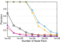
(a) Digg

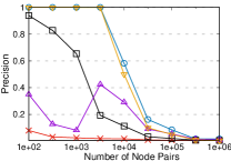
(b) Yelp

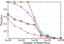
(c) Tmall

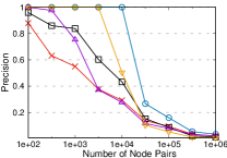
(d) DBLP

Figure 4: The precision scores achieved by different methods in the network reconstruction task.

V-A Datasets

Since the focus of this work is on temporal network representation learning, we conduct extensive experiments on four real-world datasets containing temporal information. They include one e-commerce network, one review network, one co-author network and one social network. The statistics of each dataset are summarized in Table I and the detailed descriptions are listed as follows.

• DBLP is a co-author network where each edge represents a co-authorship between two authors (nodes). We derive a subset of the co-author network which contains co-authorship between researchers from 1955 to 2017.

• Digg is a social network where each edge represents the friendship between two users (nodes) and each edge is annotated with a timestamp, indicating when this friendship is formed. The time span of the network is from 2004 to 2009.

• Tmall [14] is extracted from the sales data of the “Double 11” shopping event in 2014 at Tmall.com. Each node refers to either one user or one item and each edge refers to one purchase with a purchase date.

• Yelp [14] is extracted from the Yelp Challenge Dataset. In this network, each node either refers to one user or one business, and each comment is represented as an edge connection between users.

V-B Baseline Algorithms

We use the following four methods as the baselines.

• HTNE [14] adopted the Hawkes process [13] to model the neighborhood formation sequences where the current neighbor formation can be influenced with higher intensity by more recent events.

• Node2Vec [1] first sampled random walks with some parameters controlling inward/outward explorations (e.g., DFS and BFS) to cover both micro and macro views of neighborhoods. Then random walks are sampled to generate sequences of nodes which can be used as the input to a skip-gram model to learn the final representations.

• CTDNE [12] extended the idea of Node2Vec [1] with the skip-gram model by adding time constraints on the random walks and require nodes to co-occur in the same time-constrained random walk in order to produce similar embeddings for related nodes.

• LINE [4] optimized node representations by preserving the first-order and second-order proximity of a network. As recommended by the authors, we concatenate the representations that preserve these two proximities respectively and use the concatenated embeddings for our experiments.

V-C Parameter Settings

For our method, we set the mini-batch size, the safety margin size and the number of layers in stacked LSTM to be 512, 5 and 2 respectively. For parameters $p$ and $q$ in the time-aware random walks and the learning rate $r$, we use grid search over $p,q\in\{0.25,0.50,1,2,4\}$ and $r\in\{2\times 10^{-5},2\times 10^{-6},2\times 10^{-7}\}$ respectively. We set the number of walks $k=10$ and the walk length $l=10$ by default. Following previous work [3, 1], we set the number of negative samples to 5 for all methods and set $k=10$ and $l=80$ for Node2Vec. For CTDNE, we use the uniform sampling for initial edge selections and node selections in the random walks and set the window count to the same value used by Node2Vec. The embedding size is fixed to 128 for all methods. For all other baseline parameters, the recommended were used.

V-D Network Reconstruction

This first task we evaluate is network reconstruction, which is one of the primary problems originally explored for network embedding [2]. In this task, we train node embeddings and rank pairs of nodes using dot product similarity (one of the most common generic similarity metrics [9]) sorted in descending order. If a pair of nodes is ranked higher based on the similarity metric, an edge formed by this pair of nodes is more likely to exist in the original network. The evaluation metric $Precision@\mathcal{P}$ [9] is defined as below: $Precision@\mathcal{P}=\frac{1}{\mathcal{P}}\sum_{i=1}^{\mathcal{P}}\mu_{i}$. Here, $\mathcal{P}$ is the number of evaluated pairs. $\mu_{i}=1$ means that the edge formed by the $i-th$ reconstructed pair of nodes exists in the original network; otherwise, $\mu_{i}=0$. Since it is computationally expensive to process all possible $\frac{|\mathcal{V}|(|\mathcal{V}|-1)}{2}$ pairs of nodes, especially for large networks, we conduct evaluations on ten thousand randomly sampled nodes and repeat this process ten times and report the average $Precision@\mathcal{P}$.

Figure 4 compares the precision scores achieved by different methods on the four datasets. Our method EHNA outperforms all baselines across all datasets. More specifically, EHNA consistently outperforms HTNE and CTDNE when the number $\mathcal{P}$ of reconstruction pairs varies from $1\times 10^{2}$ to $1\times 10^{6}$, outperforms Node2Vec when $\mathcal{P}$ varies from 500 to $1\times 10^{6}$, and outperforms LINE when $\mathcal{P}$ varies from $1\times 10^{4}$ to $1\times 10^{6}$. Note that the difference w.r.t. the performance of some methods can be very small when the number of pairs of nodes is small, thus it is very hard to visually distinguish these methods. However, the difference w.r.t. the performance between EHNA and HTNE, Node2Vec or CTDNE is notable on all datasets under different cases.

All methods converge to similar performance when $\mathcal{P}$ is sufficiently large since most of the true edges which were previously ranked have already been recovered correctly. The above results show that our method can effectively capture one of the most important aspects of network structure when leveraging the available temporal information.

Operators Symbol Definition Mean $\boxplus$ $[\bm{e}_{x}\boxplus\bm{e}_{y}]_{i}=\frac{\bm{e}_{x}(i)+\bm{e}_{y}(i)}{2}$ Hadamard $\boxdot$ $[\bm{e}_{x}\boxdot\bm{e}_{y}]_{i}=\bm{e}_{x}(i)\ast\bm{e}_{y}(i)$ Weighted-L1 $\|\cdot\|_{\widehat{1}}$ $\|\bm{e}_{x}\cdot\bm{e}_{y}\|_{\widehat{1}i}=|\bm{e}_{x}(i)-\bm{e}_{y}(i)|$ Weighted-L2 $\|\cdot\|_{\widehat{2}}$ $\|\bm{e}_{x}\cdot\bm{e}_{y}\|_{\widehat{2}i}=|\bm{e}_{x}(i)-\bm{e}_{y}(i)|^{2}$

TABLE II: Choice of binary operators $\circ$ for edge representations. The definitions correspond to the $i$-th element of $\bm{e}_{(x,y)}$ and $\bm{e}_{x}(i)$ refers to the $i$-th element of $\bm{e}_{x}$.

Operator Metric LINE Node2Vec CTDNE HTNE EHNA Error Reduction Mean AUC 0.6536 0.6322 0.6308 0.6097 0.6404 -3.8% F1 0.6020 0.5870 0.6149 0.5701 0.6634 12.6% Precision 0.6184 0.6039 0.6683 0.5813 0.6881 6.0% Recall 0.5865 0.5711 0.5694 0.5593 0.6404 16.1% Hadamard AUC 0.6855 0.8680 0.9280 0.7680 0.9292 1.7% F1 0.6251 0.7969 0.8631 0.6879 0.8636 0.3% Precision 0.6370 0.8131 0.9132 0.7770 0.8808 -37.3% Recall 0.6136 0.7813 0.8182 0.6171 0.8469 15.8% Weighted-L1 AUC 0.7688 0.6788 0.9063 0.8237 0.9031 -3.4% F1 0.6938 0.5843 0.8384 0.7481 0.8273 -6.7% Precision 0.7085 0.6293 0.8276 0.7458 0.8352 4.4% Recall 0.6798 0.5506 0.8495 0.7504 0.8196 -19.9% Weighted-L2 AUC 0.7737 0.6722 0.9057 0.8211 0.9025 -3.4% F1 0.6999 0.5510 0.8296 0.7540 0.8267 -1.7% Precision 0.7119 0.6497 0.8493 0.7341 0.8092 -26.6% Recall 0.6882 0.4783 0.8107 0.7750 0.8405 19.6%

TABLE III: Different metric scores achieved by methods with different operators in the link prediction task on Digg.Error Reduction is calculated as $\frac{(1-\text{them})-(1-\text{us})}{(1-\text{them})}$ [40], where “them” refers to the best performer from baselines and “us” refers to our proposed method EHNA.

Operator Metric LINE Node2Vec CTDNE HTNE EHNA Error Reduction Mean AUC 0.7669 0.5359 0.7187 0.5167 0.7550 -5.1% F1 0.6968 0.5261 0.6715 0.4942 0.7008 1.3% Precision 0.7147 0.5275 0.7079 0.5018 0.6873 -9.6% Recall 0.6797 0.5246 0.6387 0.4868 0.7184 12.1% Hadamard AUC 0.5683 0.9359 0.9564 0.9497 0.9775 48.4% F1 0.5500 0.8648 0.8944 0.8911 0.9296 33.3% Precision 0.5506 0.8639 0.9231 0.9040 0.9207 -3.1% Recall 0.5493 0.8657 0.8674 0.8785 0.9387 49.5% Weighted-L1 AUC 0.7611 0.8713 0.8380 0.9413 0.9506 15.8% F1 0.6891 0.8119 0.7542 0.8776 0.8951 14.3% Precision 0.6980 0.7931 0.7744 0.8547 0.8739 13.2% Recall 0.6803 0.8315 0.7350 0.9016 0.9173 16.0% Weighted-L2 AUC 0.7736 0.8723 0.8296 0.9394 0.9465 11.7% F1 0.7010 0.8180 0.7280 0.8752 0.8895 11.5% Precision 0.7088 0.7877 0.7911 0.8362 0.8527 10.1% Recall 0.6933 0.8508 0.6742 0.9181 0.9296 14.0%

TABLE IV: Different metric scores achieved by methods with different operators in the link prediction task on Yelp.

Operator Metric LINE Node2Vec CTDNE HTNE EHNA Error Reduction Mean AUC 0.5198 0.5643 0.7948 0.5277 0.7858 -4.4% F1 0.5126 0.5542 0.7366 0.5182 0.7291 -2.8% Precision 0.5139 0.5495 0.7330 0.5183 0.7100 -8.6% Recall 0.5113 0.5589 0.7403 0.5180 0.7492 3.4% Hadamard AUC 0.5008 0.8890 0.8704 0.8889 0.9407 46.6% F1 0.4964 0.8142 0.7838 0.8049 0.8707 30.4% Precision 0.5000 0.8591 0.8415 0.8294 0.8420 -12.1% Recall 0.4928 0.7738 0.7336 0.7817 0.9013 54.8% Weighted-L1 AUC 0.6078 0.8205 0.6882 0.9278 0.9378 13.9% F1 0.5719 0.7407 0.6249 0.8518 0.8640 8.2% Precision 0.5754 0.7625 0.6412 0.8638 0.8617 -1.5% Recall 0.5684 0.7201 0.6093 0.8402 0.8664 16.4% Weighted-L2 AUC 0.6157 0.8239 0.6741 0.9296 0.9324 4.0% F1 0.5774 0.7439 0.6001 0.8542 0.8603 4.2% Precision 0.5798 0.7545 0.6563 0.8525 0.8617 6.2% Recall 0.5750 0.7336 0.5527 0.8559 0.8664 7.3%

TABLE V: Different metric scores achieved by methods with different operators in the link prediction task on Tmall.

Operator Metric LINE Node2Vec CTDNE HTNE EHNA Error Reduction Mean AUC 0.5685 0.5438 0.5763 0.5342 0.7362 37.7% F1 0.5462 0.5258 0.5277 0.4977 0.6735 28.1% Precision 0.5483 0.5285 0.5447 0.5099 0.6024 12.0% Recall 0.5442 0.5231 0.5116 0.4861 0.7636 48.1% Hadamard AUC 0.6726 0.8770 0.8723 0.8829 0.9113 24.3% F1 0.6256 0.8311 0.8136 0.8239 0.8562 14.9% Precision 0.6296 0.8233 0.8519 0.8274 0.8427 -6.2% Recall 0.6218 0.8391 0.7785 0.8204 0.8701 19.3% Weighted-L1 AUC 0.7147 0.8766 0.7084 0.8971 0.9341 36.0% F1 0.6532 0.8300 0.6731 0.8486 0.8857 24.5% Precision 0.6624 0.8384 0.6402 0.8466 0.8675 13.6% Recall 0.6444 0.8217 0.7095 0.8507 0.9046 36.1% Weighted-L2 AUC 0.7144 0.8775 0.7011 0.8983 0.9265 27.7% F1 0.6544 0.8364 0.6786 0.8567 0.8774 14.4% Precision 0.6599 0.8274 0.6226 0.8330 0.8561 13.8% Recall 0.6491 0.8456 0.7457 0.8817 0.8997 15.2%

TABLE VI: Different metric scores achieved by methods with different operators in the link prediction task on DBLP.

V-E Link Prediction

The link prediction task aims to predict which pairs of nodes are likely to form edges, which is an important application of network embedding. In this task, we focus on future link prediction. To simulate this problem, we remove 20% of the most recent edges in a graph, and use them for prediction. The rest of the network is used to train the model. After the training process, we use the removed edges as the positive examples and generate an equal number of negative examples by randomly sampling node pairs from the network where there are no current edge connections. After generating the positive and negative examples, we generate edge representations using the learned node embeddings and split these edge representations into a training dataset and test dataset which then are used to train the same logistic regression classifier with the LIBLINEAR package [41] to ensure that all embeddings were compared on an equal footing.

We generate edge representations with learned node embeddings based on several commonly used binary operators. More specifically, given a binary operator $\circ$, as well as two embeddings $\bm{e}_{x}$ and $\bm{e}_{y}$ of node $x$ and $y$ respectively, we generate the representation $f(x,y)$ of the edge $(x,y)$ such that $f:V\times V\rightarrow\mathbb{R}^{d}$. Here, $d=128$ is the representation size for edge $(x,y)$. Following previous work [1], we use four different operators (Table II) to generate the final edge representations. These four operators can be interpreted as four different indications of the relationships between the representations of nodes with links and nodes without links. For example, the mean operator may indicate that the averaged vectors of pairs of nodes with links should be located in similar positions in the embedding space. Similarly, the Weighted-L1 and L2 operators may indicate that the distance between nodes with links in the embedding space should be smaller than the one between nodes without links.

If the node embeddings learned by a method preserve the property or relationship indicated by a specific operator, then a classifier can easily distinguish positive edge representations (i.e., edges actually exist in the graph) from negative edge representations (i.e., edges which do not exist in the graph) generated by that operator. In the link prediction task, many existing studies have only adopted one operator for the final evaluation. Since the choice of operator may be domain specific, an effective embedding method should be robust to the choice of operators. Thus, we report the performance results under all operators defined in Table II. Some operators clearly work better than others, but we are unaware of any systematic and sensible evaluation of combining operators or how to chose the best one for network embedding problems such as link prediction. We leave this exploration to further work.

We randomly select 50% of examples as the training dataset and the rest of examples as the test dataset and train the logistic regression classifier with the LIBLINEAR package [41]. We repeat this process ten times and report the average performance. Tables III-VI compare the performance of all methods with different combining operators on each dataset. Our method EHNA significantly outperforms all other baselines in most cases. In the cases where EHNA is not the best performer, the performance of EHNA is still quite competitive, achieving the second best result. Note that we compute the error reduction by comparing EHNA with the best performer in baselines and the performance of baselines varies notably across different datasets. Thus, the performance gains of EHNA is more significant when making pairwise comparisons with certain other baselines.

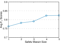
(a)

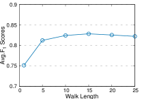
(b) Varing the walk length

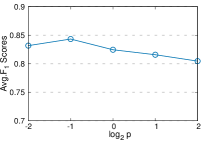
(c) Varing the value of $p$

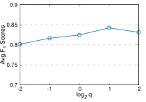
(d) Varing the value of $q$

Figure 5: Parameter sensitivity analysis of HTNE on Yelp.

V-F Ablation Study

Table VII compares the performance of different variants of EHNA in the link prediction task. Due to space limitations, we only show the performance using the Weighted-L2 operator. EHNA-NA refers to the variant without attention mechanisms, EHNA-RW refers to the variant which employs traditional random walks without an attention mechanism and EHNA-SL refers to the variant which only uses a single-layered LSTM without the two-level aggregation strategy. As we can see in Table VII, each of our proposed techniques (i.e., temporal random walks, the two-level aggregation and attention models) contributes to the effectiveness of our learned representations, and affect overall performance in downstream tasks.

Method F1 scores under Weighted-L2 Digg Yelp Tmall DBLP EHNA 0.8267 0.8895 0.8603 0.8774 EHNA-NA 0.8131 0.8714 0.8442 0.8685 EHNA-RW 0.7837 0.8446 0.8233 0.8327 EHNA-SL 0.7254 0.7784 0.7532 0.7231

TABLE VII: Performance comparisons among different variants of ENHA in the link prediction task.

Method Average running time per epoch (s) Digg Yelp Tmall DBLP Node2Vec $4.6\times 10^{3}$ $7.1\times 10^{3}$ $1.0\times 10^{4}$ $2.5\times 10^{3}$ Node2Vec_10 $4.8\times 10^{2}$ $8.8\times 10^{2}$ $1.2\times 10^{3}$ $3.2\times 10^{2}$ CTDNE $2.6\times 10^{3}$ $4.2\times 10^{3}$ $9.1\times 10^{3}$ $1.9\times 10^{3}$ CTDNE_10 $3.2\times 10^{2}$ $5.4\times 10^{2}$ $1.1\times 10^{3}$ $2.2\times 10^{2}$ Line_10 $1.2\times 10^{4}$ $1.2\times 10^{4}$ $1.2\times 10^{4}$ $1.2\times 10^{4}$ HTNE $3.8\times 10^{1}$ $5.3\times 10^{1}$ $1.1\times 10^{2}$ $1.6\times 10^{2}$ EHNA $7.8\times 10^{2}$ $1.8\times 10^{3}$ $3.2\times 10^{3}$ $1.7\times 10^{3}$

TABLE VIII: Training time comparisons.

V-G Efficiency Study

In this section, we compare the efficiency of different methods. Note that it is hard to quantify the exact running time of learning-related algorithms as there are multiple factors (e.g., initial learning rates) that can impact convergence (e.g., the number of epochs) and we did not over tune hyperparameters for any method. Instead, we explore the comparative scalability of the methods by reporting the average running time in each epoch as shown in Table VIII where Node2Vec_10, CTDNE_10 and Line_10 refer to the multi-threaded versions (i.e., 10 threads in our experiments) of the corresponding baselines. When compared to the baselines, our method EHNA is scalable and efficiency may be further improved with multi-threading. It is worth noting that Line achieved similar performance across all datasets as its efficiency depends primarily on the number of sampled edges which is the same in all experiments.

V-H Parameter Analysis

In this section, we examine how the different choices of parameters affect the performance of EHNA on the Yelp dataset with 50% as the training ratio. Excluding the parameter being evaluated, all parameters use their recommended default as discussed above.

The safety margin size. Recall that our objective function (Equation 7) aims to keep nodes with links close to each other and nodes without links far apart. The safety margin size $m$ controls how close nodes with links can be and how far nodes without links can be to each other. Thus, increasing the value of $m$ tends to lead to more accurate results. We show how $m$ influences EHNA in Figure 5a. The performance improves notably when $m$ ranges from 1 to 4 and converges when $m=5$.

The walk length of temporal random walks. The walk length is crucial to the identification of relevant nodes in historical neighborhoods as it potentially influences the number of relevant nodes and specifies the upper bound of how ‘far’ a node can be from the target node. As shown in Figure 5b, the performance improves significantly when $l$ ranges from 1 to 10, followed by subtle improvements when $l$ increases from 10 to 15. Then, the performance of EHNA slightly decays when $l$ ranges from 15 to 25. These observations suggest: (1) nodes ‘too far away‘ from the target node have little impact on the behavior of the target node, and their inclusion can introduce noise into the aggregation process, resulting in performance decay; (2) our proposed deep neural network is capable of capturing and aggregating useful information from relevant nodes and filtering noisy nodes in historical neighborhoods, but when the length of random walks become too long, the performance of our method begins to degrade.

Parameters $p$ and $q$. The parameter $p$ controls the likelihood of immediately revisiting the previous node in a walk and the parameter $q$ controls the bias towards BFS and DFS. It is interesting to see how relevant nodes are distributed in the neighborhood for different choices of $p$ and $q$. In Figure 5c, the performance of EHNA peaks when $log_{2}^{p}=-1$. In Figure 5d, the performance of EHNA peaks when $log_{2}^{q}=1$. Recall from Equation 2 that a small value of $p$ will cause the walk to backtrack and keep the walk ‘locally’ close to the starting node (i.e. the target node). A large $q$ encourages ‘inward’ explorations and BFS behavior. Thus, the observation from Figure 5c and Figure 5d indicates that the vast majority of relevant nodes reside in nearby neighborhoods in the Digg dataset. Thus, by probing the optimal values of $p$ and $q$, we can better understand the distributions of relevant nodes in different datasets.

VI Conclusion

In this paper, we studied the problem of temporal network embedding using historical neighborhood aggregation. In reality, most of networks are formed through sequential edge formations in chronological order. By exploring the most important factors influencing edge formations in certain classes of networks, we can better model the evolution of the the entire network, and induce effective feature representations that capture node influence and interactions. We first proposed a temporal random walk to identify historical neighborhoods containing nodes that are most likely to be relevant to edge formations. Then we aggregated the information from the target graph in order to analyze edge formations. Then, we introduced two optimization strategies, a two-level aggregation and attention mechanism to enable our algorithm to capture temporal information in networks. Extensive experiments on four large scale real-world networks have demonstrated the benefits of our new approach for the tasks of network reconstruction and link prediction.

Acknowledgment. This work was partially supported by ARC DP170102726, DP180102050, DP170102231, NSFC 61728204, 91646204 and Google. Guoliang Li was partially supported by the 973 Program of China (2015CB358700), NSFC (61632016, 61521002, 61661166012), Huawei, and TAL education.

References

- [1] A. Grover and J. Leskovec, “node2vec: Scalable feature learning for networks,” in SIGKDD, 2016, pp. 855–864.
- [2] D. Wang, P. Cui, and W. Zhu, “Structural deep network embedding,” in SIGKDD, 2016, pp. 1225–1234.
- [3] B. Perozzi, R. Al-Rfou, and S. Skiena, “Deepwalk: Online learning of social representations,” in SIGKDD, 2014, pp. 701–710.
- [4] J. Tang, M. Qu, M. Wang, M. Zhang, J. Yan, and Q. Mei, “Line: Large-scale information network embedding,” in WWW, 2015, pp. 1067–1077.
- [5] W. Guo, Y. Li, M. Sha, and K.-L. Tan, “Parallel personalized pagerank on dynamic graphs,” PVLDB, vol. 11, no. 1, pp. 93–106, 2017.
- [6] Y. Li, D. Zhang, Z. Lan, and K.-L. Tan, “Context-aware advertisement recommendation for high-speed social news feeding,” in ICDE, 2016, pp. 505–516.
- [7] S. Huang, Z. Bao, J. S. Culpepper, and B. Zhang, “Finding temporal influential users over evolving social networks,” in ICDE, 2019, pp. 398–409.
- [8] W. L. Hamilton, R. Ying, and J. Leskovec, “Representation learning on graphs: Methods and applications,” arXiv preprint arXiv:1709.05584, 2017.
- [9] P. Cui, X. Wang, J. Pei, and W. Zhu, “A survey on network embedding,” CoRR, vol. abs/1711.08752, 2017.
- [10] L. Zhou, Y. Yang, X. Ren, F. Wu, and Y. Zhuang, “Dynamic network embedding by modeling triadic closure process,” in AAAI, 2018, pp. 571–578.
- [11] L. Zhu, D. Guo, J. Yin, G. Ver Steeg, and A. Galstyan, “Scalable temporal latent space inference for link prediction in dynamic social networks,” TKDE, vol. 28, no. 10, pp. 2765–2777, 2016.
- [12] G. H. Nguyen, J. B. Lee, R. A. Rossi, N. K. Ahmed, E. Koh, and S. Kim, “Continuous-time dynamic network embeddings,” in Companion of WWW, 2018, pp. 969–976.
- [13] A. G. Hawkes, “Spectra of some self-exciting and mutually exciting point processes,” Biometrika, vol. 58, no. 1, pp. 83–90, 1971.
- [14] Y. Zuo, G. Liu, H. Lin, J. Guo, X. Hu, and J. Wu, “Embedding temporal network via neighborhood formation,” in SIGKDD, 2018, pp. 2857–2866.
- [15] M. Belkin and P. Niyogi, “Laplacian eigenmaps and spectral techniques for embedding and clustering,” in NeurIPS, 2002, pp. 585–591.
- [16] J. B. Kruskal, “Multidimensional scaling by optimizing goodness of fit to a nonmetric hypothesis,” Psychometrika, vol. 29, no. 1, pp. 1–27, 1964.
- [17] A. Ahmed, N. Shervashidze, S. Narayanamurthy, V. Josifovski, and A. J. Smola, “Distributed large-scale natural graph factorization,” in WWW, 2013, pp. 37–48.
- [18] S. Cao, W. Lu, and Q. Xu, “Grarep: Learning graph representations with global structural information,” in CIKM, 2015, pp. 891–900.
- [19] M. Ou, P. Cui, J. Pei, Z. Zhang, and W. Zhu, “Asymmetric transitivity preserving graph embedding,” in SIGKDD, 2016, pp. 1105–1114.
- [20] G. E. Hinton and R. R. Salakhutdinov, “Reducing the dimensionality of data with neural networks,” science, vol. 313, no. 5786, pp. 504–507, 2006.
- [21] Y. Dong, N. V. Chawla, and A. Swami, “metapath2vec: Scalable representation learning for heterogeneous networks,” in SIGKDD, 2017, pp. 135–144.
- [22] J. Tang, M. Qu, and Q. Mei, “Pte: Predictive text embedding through large-scale heterogeneous text networks,” in SIGKDD, 2015, pp. 1165–1174.
- [23] H. Chen, H. Yin, W. Wang, H. Wang, Q. V. H. Nguyen, and X. Li, “Pme: projected metric embedding on heterogeneous networks for link prediction,” in SIGKDD, 2018, pp. 1177–1186.
- [24] T. N. Kipf and M. Welling, “Semi-supervised classification with graph convolutional networks,” arXiv preprint arXiv:1609.02907, 2016.
- [25] W. Hamilton, Z. Ying, and J. Leskovec, “Inductive representation learning on large graphs,” in NeurIPS, 2017, pp. 1024–1034.
- [26] J. Bruna, W. Zaremba, A. Szlam, and Y. LeCun, “Spectral networks and locally connected networks on graphs,” arXiv preprint arXiv:1312.6203, 2013.
- [27] T. N. Kipf and M. Welling, “Variational graph auto-encoders,” arXiv preprint arXiv:1611.07308, 2016.
- [28] M. Schlichtkrull, T. N. Kipf, P. Bloem, R. van den Berg, I. Titov, and M. Welling, “Modeling relational data with graph convolutional networks,” in European Semantic Web Conference, 2018, pp. 593–607.
- [29] R. van den Berg, T. N. Kipf, and M. Welling, “Graph convolutional matrix completion,” CoRR, vol. abs/1706.02263, 2017.
- [30] T. Pham, T. Tran, D. Phung, and S. Venkatesh, “Column networks for collective classification,” in AAAI, 2017.
- [31] P. Velickovic, G. Cucurull, A. Casanova, A. Romero, P. Liò, and Y. Bengio, “Graph attention networks,” in ICLR, 2018.
- [32] H. Chen, H. Yin, T. Chen, Q. V. H. Nguyen, W.-C. Peng, and X. Li, “Exploiting centrality information with graph convolutions for network representation learning,” in ICDE, 2019.
- [33] S. Ioffe and C. Szegedy, “Batch normalization: Accelerating deep network training by reducing internal covariate shift,” in ICML, 2015, pp. 448–456.
- [34] D. Bahdanau, K. Cho, and Y. Bengio, “Neural machine translation by jointly learning to align and translate,” in ICLR, 2015.
- [35] K. He, X. Zhang, S. Ren, and J. Sun, “Identity mappings in deep residual networks,” in ECCV, 2016, pp. 630–645.
- [36] C.-K. Hsieh, L. Yang, Y. Cui, T.-Y. Lin, S. Belongie, and D. Estrin, “Collaborative metric learning,” in WWW, 2017, pp. 193–201.
- [37] N. Shervashidze, P. Schweitzer, E. J. v. Leeuwen, K. Mehlhorn, and K. M. Borgwardt, “Weisfeiler-lehman graph kernels,” Journal of Machine Learning Research, vol. 12, no. Sep, pp. 2539–2561, 2011.
- [38] T. Mikolov, I. Sutskever, K. Chen, G. S. Corrado, and J. Dean, “Distributed representations of words and phrases and their compositionality,” in NeurIPS, 2013, pp. 3111–3119.
- [39] H. Yin, H. Chen, X. Sun, H. Wang, Y. Wang, and Q. V. H. Nguyen, “Sptf: a scalable probabilistic tensor factorization model for semantic-aware behavior prediction,” in ICDM, 2017, pp. 585–594.
- [40] S. Abu-El-Haija, B. Perozzi, R. Al-Rfou, and A. A. Alemi, “Watch your step: Learning node embeddings via graph attention,” in NeurIPS, 2018, pp. 9180–9190.
- [41] R.-E. Fan, K.-W. Chang, C.-J. Hsieh, X.-R. Wang, and C.-J. Lin, “Liblinear: A library for large linear classification,” Journal of machine learning research, vol. 9, no. Aug, pp. 1871–1874, 2008.