Abstract

Permutation tests are widely used in statistics, providing a finite-sample guarantee on the type I error rate whenever the distribution of the samples under the null hypothesis is invariant to some rearrangement. Despite its increasing popularity and empirical success, theoretical properties of the permutation test, especially its power, have not been fully explored beyond simple cases. In this paper, we attempt to partly fill this gap by presenting a general non-asymptotic framework for analyzing the minimax power of the permutation test. The utility of our proposed framework is illustrated in the context of two-sample and independence testing under both discrete and continuous settings. In each setting, we introduce permutation tests based on $U$-statistics and study their minimax performance. We also develop exponential concentration bounds for permuted $U$-statistics based on a novel coupling idea, which may be of independent interest. Building on these exponential bounds, we introduce permutation tests which are adaptive to unknown smoothness parameters without losing much power. The proposed framework is further illustrated using more sophisticated test statistics including weighted $U$-statistics for multinomial testing and Gaussian kernel-based statistics for density testing. Finally, we provide some simulation results that further justify the permutation approach.

1 Introduction

A permutation test is a nonparametric approach to hypothesis testing routinely used in a variety of scientific applications such as astronomy (Efron and Petrosian,, 1992; Freeman et al.,, 2017), biology (Pesarin,, 2001; Blackford et al.,, 2009), neuroscience (Hayasaka and Nichols,, 2004; Maris and Oostenveld,, 2007) and genomics (Stranger et al.,, 2007; Maglietta et al.,, 2007). The permutation test constructs the resampling distribution of a test statistic by permuting the labels of the observations. The resampling distribution, also called the permutation distribution, serves as a reference from which to assess the significance of the observed test statistic. A key property of the permutation test is that it provides exact control of the type I error rate for any test statistic whenever the labels are exchangeable under the null hypothesis (e.g. Hoeffding,, 1952). Due to this attractive non-asymptotic property, the permutation test has received considerable attention and has been applied to a wide range of statistical tasks including testing independence, two-sample testing, change point detection, clustering, classification, principal component analysis (see Anderson and Robinson,, 2001; Kirch and Steinebach,, 2006; Park et al.,, 2009; Ojala and Garriga,, 2010; Zhou et al.,, 2018).

Once the type I error is controlled, the next concern is the type II error or equivalently the power of the resulting test. Despite its increasing popularity and empirical success, the power of the permutation test has yet to be fully understood. A major challenge in this regard is to control its random critical value that can have an intractable distribution. More specifically, in order to show that a test has high power, we need to ensure that the distribution of the test statistic is significantly distant from its critical value under the alternative. For the permutation test, this critical value is a random quantity, defined as a quantile of the permutation distribution. Studying this random value is in general difficult due to the combinatorial nature of the permutation distribution. While some progress has been made as we review in Section 1.2, our understanding of the permutation approach is still far from complete, especially in finite-sample scenarios. The purpose of this paper is to attempt to partly fill this gap by developing a general framework for analyzing the non-asymptotic minimax type II error of the permutation test. Using the tools developed in this paper, we demonstrate that permutation tests are minimax rate optimal in various scenarios.

1.1 Alternative approaches and their limitations

We first review a couple of other testing procedures and highlight the advantages of the permutation method. One common approach to determining the critical value of a test is based on the asymptotic null distribution of a test statistic. The validity of a test whose rejection region is calibrated using this asymptotic null distribution is well-studied in the classical regime where the number of parameters is held fixed and the sample size goes to infinity. However, it is no longer trivial to justify this asymptotic approach in a complex, high-dimensional setting where numerous parameters can interact in a non-trivial way and strongly influence the behavior of the test statistic. In such a case, the limiting null distribution is perhaps intractable without imposing stringent assumptions. To illustrate the challenge clearly, we consider the two-sample $U$-statistic $U_{n_{1},n_{2}}$ defined later in Proposition 4.3 for multinomial testing. Here we compute $U_{n_{1},n_{2}}$ based on samples from the multinomial distribution with uniform probabilities. To approximate the null distribution of $U_{n_{1},n_{2}}$, we perform 1000 Monte-Carlo simulations for each number of bins $d\in\{5,100,10000\}$ while fixing the sample sizes as $n_{1}=n_{2}=100$. From the histograms in Figure 1, we see that the shape of the null distribution heavily depends on the number of bins $d$ (and more generally on the probabilities of the null multinomial distribution). In particular, the null distribution tends to be more symmetric and sparser as $d$ increases. Since the underlying structure of the distribution is unknown beforehand, Figure 1 emphasizes difficulties of approximating the null distribution over different regimes. This in turn has led statisticians to impose stringent assumptions under which test statistics have simple, tractable limiting distributions. However, as noted in Balakrishnan and Wasserman, (2018), this can exclude many high-dimensional cases when – despite having non-normal null distributions – carefully designed tests can have high (minimax) power. We also note that the asymptotic approach does not have any finite sample guarantee, which is also true for other data-driven methods including bootstrapping (Efron and Tibshirani,, 1994) and subsampling (Politis et al.,, 1999). In sharp contrast, the permutation approach provides a valid test for any test statistic in any sample size under minimal assumptions. Furthermore, as we shall see, one can achieve minimax power through the permutation test even when a nice limiting null distribution is not available.

Another approach, that is commonly used in theoretical computer science, is based on concentration inequalities (e.g. Chan et al.,, 2014; Acharya et al.,, 2014; Bhattacharya and Valiant,, 2015; Diakonikolas and Kane,, 2016; Canonne et al.,, 2018). In this approach the threshold of a test is determined using a tail bound of the test statistic under the null hypothesis. Then, owing to the non-asymptotic nature of the concentration bound, the resulting test can control the type I error rate in finite samples. This non-asymptotic approach is more robust to distributional assumptions than the previous asymptotic approach but comes with different challenges. For instance the resulting test tends to be too conservative as it depends on a loose tail bound. A more serious problem is that the threshold often relies on unspecified constants and even unknown parameters. By contrast, the permutation approach is entirely data-dependent and tightly controls the type I error rate.

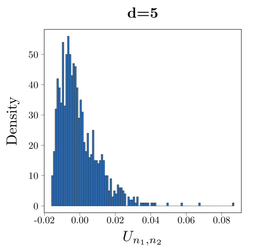
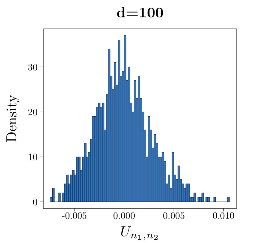
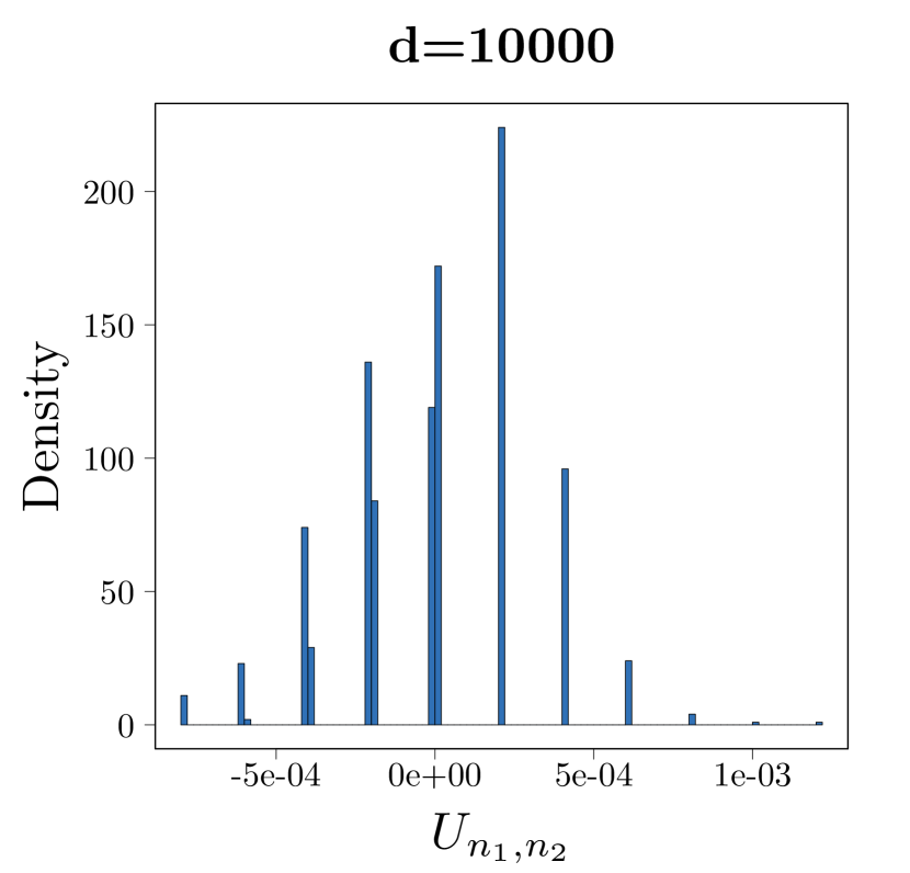
Figure 1: Histograms of the $U$-statistic in Proposition 4.3 calculated under the uniform multinomial null by varying the number of bins $d$. The plots show that the shape of the null distribution is highly influenced by the number of bins and thus illustrate challenges of estimating the null distribution consistently over different scenarios. See Section 1.1 for details.

1.2 Challenges in power analysis and related work

Having motivated the importance of the permutation approach, we now review the previous studies on permutation tests and also discuss challenges. The large sample power of the permutation test has been investigated by a number of authors including Hoeffding, (1952); Robinson, (1973); Albers et al., (1976); Bickel and van Zwet, (1978); Janssen, (1997). The main result in this line of research indicates that the permutation distribution of a certain test statistic (e.g. Student’s $t$-statistic and $F$-statistic) approximates its null distribution in large sample scenarios. Moreover this approximation is valid under both the null and local alternatives, which then guarantees that the permutation test is asymptotically as powerful as the test based on the asymptotic null distribution. In addition to these findings, power comparisons between permutation and bootstrap tests have been made by Romano, (1989); Janssen and Pauls, (2003); Janssen, (2005) and among others. However these power analyses, which rely heavily on classical asymptotic theory, are not easily generalized to more complex settings. In particular, they often require that alternate distributions satisfy certain regularity conditions under which the asymptotic power function is analytically tractable. Due to such restrictions, the focus has been on a limited class of test statistics applied to a relatively small set of distributions. Furthermore, most previous studies have studied the pointwise, instead of uniform, power that holds for any fixed sequence of alternatives but not uniformly over the class of alternatives.

Recently, there has been another line of research studying the power of the permutation test from a non-asymptotic point of view (e.g. Albert,, 2015, 2019; Kim et al.,, 2020, 2019). This framework, based on a concentration bound for a permuted test statistic, allows us to study the power in more general and complex settings than the asymptotic approach at the expense of being less precise (mainly in terms of constant factors). The main challenge in the non-asymptotic analysis, however, is to control the random critical value of the test. The distribution of this random critical value is in general difficult to study due to the non-i.i.d. structure of the permuted test statistic. Several attempts have been made to overcome such difficulty focusing on linear-type statistics (Albert,, 2019), regressor-based statistics (Kim et al.,, 2019), the Cramér–von Mises statistic (Kim et al.,, 2020) and maximum-type kernel-based statistics (Kim,, 2021). Our work contributes to this line of research by developing some general tools for studying the finite-sample performance of permutation tests with a specific focus on degenerate $U$-statistics.

Concurrent with our work, and independently, Berrett et al., (2021) also develop results for the permutation test based on a degenerate $U$-statistic. While focusing on independence testing, Berrett et al., (2021) prove that one cannot hope to have a valid independence test that is uniformly powerful over alternatives in the $L_{2}$ distance. The authors then impose Sobolev-type smoothness conditions as well as boundedness conditions on density functions under which the proposed permutation test is minimax rate optimal in the $L_{2}$ distance.

Finally, we also note that the robustness of permutation tests to violations of the exchangeability condition has been investigated by Romano, (1990); Janssen, (1997); Chung and Romano, (2013); Pauly et al., (2015); Chung and Romano, (2016); DiCiccio and Romano, (2017).

1.3 Overview of our results

In this paper we take the non-asymptotic point of view as in Albert, (2015) and establish general results to shed light on the power of permutation tests under a variety of scenarios. To concretely demonstrate our results, we focus on two canonical testing problems: 1) two-sample testing and 2) independence testing, for which the permutation approach rigorously controls the type I error rate (Section 2 for specific settings). These topics have been explored by a number of researchers across diverse fields including statistics and computer science and several optimal tests have been proposed in the minimax sense (e.g. Chan et al.,, 2014; Bhattacharya and Valiant,, 2015; Diakonikolas and Kane,, 2016; Arias-Castro et al.,, 2018). Nevertheless the existing optimal tests are mostly of theoretical interest, depending on loose or practically infeasible critical values. Motivated by this gap between theory and practice, the primary goal of this study is to introduce permutation tests that tightly control the type I error rate and have the same optimality guarantee as the existing optimal tests.

We summarize the major contributions of this paper and contrast them with the previous studies as follows:

• Two moments method (Lemma 3.1). Leveraging the quantile approach introduced by Fromont et al., (2013) (see Section 3 for details), we first present a general sufficient condition under which the permutation test has non-trivial power. This condition only involves the first two moments of a test statistic, hence called the two moments method. To make this general condition more concrete, we consider degenerate $U$-statistics for two-sample testing and independence testing, respectively, and provide simple moment conditions that ensure that the resulting permutation test has non-trivial power for each testing problem. We then illustrate the efficacy of our results with concrete examples.

• Multinomial testing (Proposition 4.3 and Proposition 5.3). One example that we focus on is multinomial testing in the $\ell_{2}$ distance. Chan et al., (2014) study the multinomial two-sample problem in the $\ell_{2}$ distance but with some unnecessary conditions (e.g. equal sample size, Poisson sampling, known squared norms etc). We remove these conditions and propose a permutation test that is minimax rate optimal for the two-sample problem. Similarly we introduce a minimax optimal test for independence testing in the $\ell_{2}$ distance based on the permutation procedure.

• Density testing (Proposition 4.6 and Proposition 5.6). Another example that we focus on is density testing for Hölder classes. Building on the work of Ingster, (1987), the two-sample problem for Hölder densities has been recently studied by Arias-Castro et al., (2018) and the authors propose an optimal test in the minimax sense. However their test depends on a loose critical value and also assumes equal sample sizes. We propose an alternative test based on the permutation procedure without such restrictions and show that it achieves the same minimax optimality. We also contribute to the literature by presenting an optimal permutation test for independence testing over Hölder classes.

• Combinatorial concentration inequalities (Theorem 6.1, Theorem 6.2 and Theorem 6.3). Although our two moments method is general, it might be sub-optimal in terms of the dependence on a nominal level $\alpha$. Focusing on degenerate $U$-statistics, we improve the dependence on $\alpha$ from polynomial to logarithmic with some extra assumptions. To do so, we develop combinatorial concentration inequalities inspired by the symmetrization trick (Duembgen,, 1998) and Hoeffding’s average (Hoeffding,, 1963). We apply the developed inequalities to introduce adaptive tests to unknown smoothness parameters at the cost of $\log\log n$ factor. In contrast to the previous studies (e.g. Chatterjee,, 2007; Bercu et al.,, 2015; Albert,, 2019) that are restricted to simple linear statistics, the proposed combinatorial inequalities are broadly applicable to the class of degenerate $U$-statistics. These results have potential applications beyond the problems considered in this paper (e.g. providing concentration inequalities under sampling without replacement).

In addition to the testing problems mentioned above, we also contribute to multinomial testing problems in the $\ell_{1}$ distance (e.g. Chan et al.,, 2014; Bhattacharya and Valiant,, 2015; Diakonikolas and Kane,, 2016). First we revisit the chi-square test for multinomial two-sample testing considered in Chan et al., (2014) and show that the test based on the same test statistic but calibrated by the permutation procedure is also minimax rate optimal under Poisson sampling (Theorem 8.1). Next, motivated by the flattening idea in Diakonikolas and Kane, (2016), we introduce permutation tests based on weighted $U$-statistics and prove their minimax rate optimality for multinomial testing in the $\ell_{1}$ distance (Proposition 8.2 and Proposition 8.3). Lastly, building on the recent work of Albert et al., (2022), we analyze the permutation tests based on the maximum mean discrepancy (Gretton et al.,, 2012) and the Hilbert–Schmidt independence criterion (Gretton et al.,, 2005) for two-sample and independence testing, respectively, and illustrate their performance over certain Sobolev-type smooth function classes.

1.4 Outline of the paper

The remainder of the paper is organized as follows. Section 2 describes the problem setting and provides some background on the permutation procedure and minimax optimality. In Section 3, we give a general condition based on the first two moments of a test statistic under which the permutation test has non-trivial power. We concretely illustrate this condition using degenerate $U$-statistics for two-sample testing in Section 4 and for independence testing in Section 5. Section 6 is devoted to combinatorial concentration bounds for permuted $U$-statistics. Building on these results, we propose adaptive tests to unknown smoothness parameters in Section 7. The proposed framework is further demonstrated using more sophisticated statistics in Section 8. We present some simulation results that justify the permutation approach in Section 9 before concluding the paper in Section 10. Additional results including concentration bounds for permuted linear statistics and the proofs omitted from the main text are provided in the appendices.

Notation.

We use the notation $X\overset{d}{=}Y$ to denote that $X$ and $Y$ have the same distribution. The set of all possible permutations of $\{1,\ldots,n\}$ is denoted by $\mathbf{\Pi}_{n}$. For two deterministic sequences $a_{n}$ and $b_{n}$, we write $a_{n}\asymp b_{n}$ if $a_{n}/b_{n}$ is bounded away from zero and $\infty$ for large $n$. For integers $p,q$ such that $1\leq q\leq p$, we let $(p)_{q}=p(p-1)\cdots{(p-q+1)}$. We use $\mathbf{i}_{q}^{p}$ to denote the set of all $q$-tuples drawn without replacement from the set $\{1,\ldots,p\}$. $C,C_{1},C_{2},\ldots,$ refer to positive absolute constants whose values may differ in different parts of the paper. We denote a constant that might depend on fixed parameters $\theta_{1},\theta_{2},\theta_{3},\ldots$ by $C(\theta_{1},\theta_{2},\theta_{3},\ldots)$. Given positive integers $p$ and $q$, we define $\mathbb{S}_{p}:=\{1,\ldots,p\}$ and similarly $\mathbb{S}_{p,q}:=\{1,\ldots,p\}\times\{1,\ldots,q\}$.

2 Background

We start by formulating the problem of interest. Let $\mathcal{P}_{0}$ and $\mathcal{P}_{1}$ be two disjoint sets of distributions (or pairs of distributions) on a common measurable space. We are interested in testing whether the underlying data generating distributions belong to $\mathcal{P}_{0}$ or $\mathcal{P}_{1}$ based on mutually independent samples $\mathcal{X}_{n}:=\{X_{1},\ldots,X_{n}\}$. Two specific examples of $\mathcal{P}_{0}$ and $\mathcal{P}_{1}$ are:

1. Two-sample testing. Let $(P_{Y},P_{Z})$ be a pair of distributions that belongs to a certain family of pairs of distributions $\mathcal{P}$. Suppose we observe $\mathcal{Y}_{n_{1}}:=\{Y_{1},\ldots,Y_{n_{1}}\}\overset{\text{i.i.d.}}{\sim}P_{Y}$ and, independently, $\mathcal{Z}_{n_{2}}:=\{Z_{1},\ldots,Z_{n_{2}}\}\overset{\text{i.i.d.}}{\sim}P_{Z}$ and denote the pooled samples by $\mathcal{X}_{n}:=\mathcal{Y}_{n_{1}}\cup\mathcal{Z}_{n_{2}}$. Given the samples, two-sample testing is concerned with distinguishing the hypotheses:

   $$H_{0}:P_{Y}=P_{Z}\quad\text{versus}\quad H_{1}:\delta(P_{Y},P_{Z})\geq\epsilon_{n_{1},n_{2}},$$

   where $\delta(P_{Y},P_{Z})$ is a certain distance between $P_{Y}$ and $P_{Z}$ and $\epsilon_{n_{1},n_{2}}>0$. In this case, $\mathcal{P}_{0}$ is the set of $(P_{Y},P_{Z})\in\mathcal{P}$ such that $P_{Y}=P_{Z}$, whereas $\mathcal{P}_{1}:=\mathcal{P}_{1}(\epsilon_{n_{1},n_{2}})$ is another set of $(P_{Y},P_{Z})\in\mathcal{P}$ such that $\delta(P_{Y},P_{Z})\geq\epsilon_{n_{1},n_{2}}$.

2. Independence testing. Let $P_{YZ}$ be a joint distribution of $Y$ and $Z$ that belongs to a certain family of distributions $\mathcal{P}$. Let $P_{Y}P_{Z}$ denote the product of their marginal distributions. Suppose we observe $\mathcal{X}_{n}:=((Y_{1},Z_{1}),\ldots,(Y_{n},Z_{n}))\overset{\text{i.i.d.}}{\sim}P_{YZ}$. Given the samples, the hypotheses for testing independence are

   $$H_{0}:P_{YZ}=P_{Y}P_{Z}\quad\text{versus}\quad H_{1}:\delta(P_{YZ},P_{Y}P_{Z})\geq\epsilon_{n},$$

   where $\delta(P_{YZ},P_{Y}P_{Z})$ is a certain distance between $P_{YZ}$ and $P_{Y}P_{Z}$ and $\epsilon_{n}>0$. In this case, $\mathcal{P}_{0}$ is the set of $P_{YZ}\in\mathcal{P}$ such that $P_{YZ}=P_{Y}P_{Z}$, whereas $\mathcal{P}_{1}:=\mathcal{P}_{1}(\epsilon_{n})$ is another set of $P_{YZ}\in\mathcal{P}$ such that $\delta(P_{YZ},P_{Y}P_{Z})\geq\epsilon_{n}$.

Let us consider a generic test statistic $T_{n}:=T_{n}(\mathcal{X}_{n})$, which is designed to distinguish between the null and alternative hypotheses based on $\mathcal{X}_{n}$. Given a critical value $c_{n}$ and pre-specified constants $\alpha\in(0,1)$ and $\beta\in(0,1-\alpha)$, the problem of interest is to find sufficient conditions on $\mathcal{P}_{0}$ and $\mathcal{P}_{1}$ under which the type I and II errors of the test $\mathds{1}(T_{n}>c_{n})$ are uniformly bounded as

$$\bullet~{}\text{Type I error:}~{}\sup_{P\in\mathcal{P}_{0}}\mathbb{P}_{P}^{(n)}\left(T_{n}>c_{n}\right)\leq\alpha,$$ (1)

$$\bullet~{}\text{Type II error:}~{}\sup_{P\in\mathcal{P}_{1}}\mathbb{P}_{P}^{(n)}\left(T_{n}\leq c_{n}\right)\leq\beta.$$

Our goal is to control these uniform (rather than pointwise) errors based on data-dependent critical values determined by the permutation procedure.

2.1 Permutation procedure

This section briefly overviews the permutation procedure and its well-known theoretical properties, referring readers to Lehmann and Romano, (2006); Pesarin and Salmaso, (2010) for more details. Let us begin with some notation. Given a permutation $\pi:=(\pi_{1},\ldots,\pi_{n})\in\mathbf{\Pi}_{n}$, we denote the permuted version of $\mathcal{X}_{n}$ by $\mathcal{X}_{n}^{\pi}$, that is, $\mathcal{X}_{n}^{\pi}:=\{X_{\pi_{1}},\ldots,X_{\pi_{n}}\}$. For the case of independence testing, $\mathcal{X}_{n}^{\pi}$ is defined by permuting the second variable $Z$, i.e. $\mathcal{X}_{n}^{\pi}:=\{(Y_{1},Z_{\pi_{1}}),\ldots,(Y_{n},Z_{\pi_{n}})\}$. We write $T_{n}^{\pi}:=T_{n}(\mathcal{X}_{n}^{\pi})$ to denote the test statistic computed based on $\mathcal{X}_{n}^{\pi}$. Let $F_{T_{n}^{\pi}}(t)$ be the permutation distribution function of $T_{n}^{\pi}$ defined as

$$F_{T_{n}^{\pi}}(t):=M_{n}^{-1}\sum\nolimits_{\pi\in\mathbf{\Pi}_{n}}\mathds{1}\{T_{n}(\mathcal{X}_{n}^{\pi})\leq t\}.$$

Here $M_{n}$ denotes the cardinality of $\mathbf{\Pi}_{n}$. We write the $1-\alpha$ quantile of $F_{T_{n}^{\pi}}$ by $c_{1-\alpha,n}$ defined as

$$c_{1-\alpha,n}:=\inf\{t:F_{T_{n}^{\pi}}(t)\geq 1-\alpha\}.$$ (2)

Given the quantile $c_{1-\alpha,n}$, the permutation test rejects the null hypothesis when $T_{n}>c_{1-\alpha,n}$. This choice of the critical value provides finite-sample type I error control under the permutation-invariant assumption (or exchangeability). In more detail, the distribution of $\mathcal{X}_{n}$ is said to be permutation invariant if $\mathcal{X}_{n}$ and $\mathcal{X}_{n}^{\pi}$ have the same distribution whenever the null hypothesis is true. This permutation-invariance holds for two-sample and independence testing problems. When permutation-invariance holds, it is well-known that the permutation test $\mathds{1}(T_{n}>c_{1-\alpha,n})$ has level $\alpha$, and by randomizing the test function we can also ensure it has size $\alpha$ (see e.g. Hoeffding,, 1952; Lehmann and Romano,, 2006; Hemerik and Goeman,, 2018).

Remark 2.1 (Computational aspects).

Exact calculation of the critical value (2) is computationally prohibitive except for small sample sizes. Therefore it is common practice to use Monte Carlo simulations to approximate the critical value (e.g. Romano and Wolf,, 2005). We note that this approximation error can be made arbitrary small by taking a sufficiently large number of Monte Carlo samples. We make this argument more rigorous in Appendix D and show that our master theorem for the permutation test (Lemma 3.1) also holds for its Monte Carlo counterpart as long as the number of Monte Carlo samples is greater than some constant that only depends on the pre-specified error rates $\alpha$ and $\beta$.

2.2 Minimax optimality

A complementary aim of this paper is to show that the sufficient conditions for the error bounds in (LABEL:Eq:_uniform_error_control) are indeed necessary in some applications. We approach this problem from the minimax perspective pioneered by Ingster, (1987), and further developed in subsequent works (Ingster and Suslina,, 2003; Ingster,, 1993; Baraud,, 2002; Lepski and Spokoiny,, 1999). Let us define a test $\phi$, which is a Borel measurable map, $\phi:\mathcal{X}_{n}\mapsto\{0,1\}$. For a class of null distributions $\mathcal{P}_{0}$, we denote the set of all level $\alpha$ tests by

$$\Phi_{n,\alpha}:=\bigg{\{}\phi:\sup_{P\in\mathcal{P}_{0}}\mathbb{P}_{P}^{(n)}\left(\phi=1\right)\leq\alpha\bigg{\}}.$$

Consider a class of alternative distributions $\mathcal{P}_{1}(\epsilon_{n})$ associated with a positive sequence $\epsilon_{n}$. Two specific examples of this class of interest are $\displaystyle\mathcal{P}_{1}(\epsilon_{n_{1},n_{2}}):=\{(P_{Y},P_{Z})\in\mathcal{P}:\delta(P_{Y},P_{Z})\geq\epsilon_{n_{1},n_{2}}\}$ for two-sample testing and $\displaystyle\mathcal{P}_{1}(\epsilon_{n}):=\{P_{YZ}\in\mathcal{P}:\delta(P_{YZ},P_{Y}P_{Z})\geq\epsilon_{n}\}$ for independence testing. Given $\mathcal{P}_{1}(\epsilon_{n})$, the maximum type II error of a test $\phi\in\Phi_{n,\alpha}$ is

$$R_{n,\epsilon_{n}}(\phi):=\sup_{P\in\mathcal{P}_{1}(\epsilon_{n})}\mathbb{P}_{P}^{(n)}(\phi=0),$$

and the minimax risk is defined as

$$R_{n,\epsilon_{n}}^{\dagger}:=\inf_{\phi\in\Phi_{n,\alpha}}R_{n,\epsilon_{n}}(\phi).$$

The minimax risk is frequently investigated via the minimum separation (or the critical radius), which is the smallest $\epsilon_{n}$ such that type II error becomes non-trivial. Formally, for some fixed $\beta\in(0,1-\alpha)$, the minimum separation is defined as

$$\epsilon_{n}^{\dagger}:=\inf\Big{\{}\epsilon_{n}:R_{n,\epsilon_{n}}^{\dagger}\leq\beta\Big{\}}.$$

Of course, it is infeasible to obtain an optimal test that achieves the exact minimax risk in most realistic cases. We instead use the yardstick of minimax rate optimality in order to assess the permutation procedure. Formally, consider a level $\alpha$ test $\phi\in\Phi_{n,\alpha}$. We call $\phi$ minimax rate optimal with separation rate $r_{n}\asymp\epsilon_{n}^{\dagger}$ if the following statement is true for every $n$: there exists an absolute constant $C>0$ such that, if $\epsilon_{n}\geq Cr_{n}$, then $R_{n,\epsilon_{n}}(\phi)\leq\beta$. This optimality guarantee is non-asymptotic and holds for every $n$.

Next we present a few remarks on the minimax framework and other testing procedures.

Remark 2.2.

• In this paper, we focus on the minimax framework to evaluate the performance of tests. The minimax framework enables us to study the fundamental limits of hypothesis testing while ensuring a (strong) uniform guarantee over a large class of (null and alternate) distributions. The notion of minimax performance is widely used to quantify the difficulty of a statistical problem. In the hypothesis testing literature, it is also common to study the performance of tests against fixed or directional alternatives. As discussed in past work (see e.g. Arias-Castro et al.,, 2018, for a discussion), consistency against fixed or directional alternatives can be misleading and can conceal the curse-of-dimensionality that we would typically expect in non-parametric or high-dimensional settings. On the other hand, when we have additional prior information suggesting alternative hypotheses of importance, a naïve use of the minimax framework to design or assess tests may not be adequate. It is certainly possible that a global minimax optimal test may not perform well against a particular fixed alternative (see e.g. our prior work Balakrishnan and Wasserman,, 2019, for empirical results). Although we restrict our attention to minimax optimality, it would also be interesting to consider other criteria (e.g. robustness, computational costs, high power against pre-specified alternatives) to assess the performance of tests. We leave this direction to future work.

• Besides the permutation procedure, bootstrap sampling and subsampling are two common practical ways of determining critical values. However, as mentioned earlier, they are only valid in a limited asymptotic setting where the test statistic has a nice limiting distribution. Therefore the tests based on these asymptotic methods do not belong to $\Phi_{n,\alpha}$ in general, and thus are often not minimax optimal in our framework.

With this background in place, we now focus on showing the minimax rate optimality of permutation tests in various settings.

3 A general strategy with first two moments

In this section, we discuss a general strategy for studying the testing errors of a permutation test based on the first two moments of a test statistic. As mentioned earlier, the permutation test is level $\alpha$ as long as permutation-invariance holds under the null hypothesis. Therefore we focus on the type II error rate and provide sufficient conditions under which the error bounds given in (LABEL:Eq:_uniform_error_control) are fulfilled. Previous approaches to non-asymptotic minimax power analysis, reviewed in Section 1.1, use a non-random critical value, often derived through upper bounds on the mean and variance of the test statistic under the null, and thus do not directly apply to the permutation test. To bridge the gap, we consider a deterministic quantile value that serves as a proxy for the permutation threshold $c_{1-\alpha,n}$. More precisely, let $q_{1-\gamma,n}$ be the $1-\gamma$ quantile of the distribution of the random critical value $c_{1-\alpha,n}$. Then by splitting the cases into $\{c_{1-\alpha,n}\leq q_{1-\gamma,n}\}$ and $\{c_{1-\alpha,n}>q_{1-\gamma,n}\}$ and using the definition of the quantile, it can be shown that the type II error of the permutation test is less than or equal to

$$\sup_{P\in\mathcal{P}_{1}}\mathbb{P}_{P}\left(T_{n}\leq c_{1-\alpha,n}\right)\leq\sup_{P\in\mathcal{P}_{1}}\mathbb{P}_{P}\left(T_{n}\leq q_{1-\gamma,n}\right)+\gamma.$$

Consequently, if one succeeds in showing that $\sup_{P\in\mathcal{P}_{1}}\mathbb{P}_{P}\left(T_{n}\leq q_{1-\gamma,n}\right)\leq\gamma^{\prime}$ with $\gamma^{\prime}$ such that $\gamma^{\prime}+\gamma\leq\beta$, then the type II error of the permutation test is bounded by $\beta$ as desired. This quantile approach to dealing with a random threshold is not new and has been considered by Fromont et al., (2013) to study the power of a kernel-based test via a wild bootstrap method. In the next lemma, we build on this quantile approach and study the testing errors of the permutation test based on an arbitrary test statistic. Here and hereafter, we denote the expectation and variance of $T_{n}^{\pi}$ with respect to the permutation distribution by $\mathbb{E}_{\pi}[T_{n}^{\pi}|\mathcal{X}_{n}]$ and $\text{Var}_{\pi}[T_{n}^{\pi}|\mathcal{X}_{n}]$, respectively.

Lemma 3.1 (Two moments method).

Suppose that for each permutation $\pi\in\mathbf{\Pi}_{n}$, $T_{n}$ and $T_{n}^{\pi}$ have the same distribution under the null hypothesis. Given pre-specified error rates $\alpha\in(0,1)$ and $\beta\in(0,1-\alpha)$, assume that for any $P\in\mathcal{P}_{1}$,

$$\mathbb{E}_{P}[T_{n}]~{}\geq{} \mathbb{E}_{P}[\mathbb{E}_{\pi}\{T_{n}^{\pi}|\mathcal{X}_{n}\}]+\sqrt{\frac{3\emph{\text{Var}}_{P}[\mathbb{E}_{\pi}\{T_{n}^{\pi}|\mathcal{X}_{n}\}]}{\beta}}$$ (3)

$$+\sqrt{\frac{3\emph{\text{Var}}_{P}[T_{n}]}{\beta}}+\sqrt{\frac{3\mathbb{E}_{P}[\emph{\text{Var}}_{\pi}\{T_{n}^{\pi}|\mathcal{X}_{n}\}]}{\alpha\beta}}.$$

Then the permutation test $\mathds{1}(T_{n}>c_{1-\alpha,n})$ controls the type I and II error rates as in (LABEL:Eq:_uniform_error_control).

The proof of this general statement follows by simple set algebra along with Markov and Chebyshev’s inequalities. The details can be found in Appendix E. At a high-level, the sufficient condition (3) roughly says that if the expected value of $T_{n}$ (say, signal) is much larger than the expected value of the permuted statistic $T_{n}^{\pi}$ (say, baseline) as well as the variances of $T_{n}$ and $T_{n}^{\pi}$ (say, noise), then the permutation test will have non-trivial power. We provide an illustration of Lemma 3.1 in Figure 2. Suppose further that $T_{n}^{\pi}$ is centered at zero under the permutation law, i.e. $\mathbb{E}_{\pi}[T_{n}^{\pi}|\mathcal{X}_{n}]=0$. Then a modification of the proof of Lemma 3.1 yields a simpler condition with improved constant factors. We show that if,

$$\mathbb{E}_{P}[T_{n}]~{}\geq~{}\sqrt{\frac{2\text{Var}_{P}[T_{n}]}{\beta}}+\sqrt{\frac{2\mathbb{E}_{P}[\text{Var}_{\pi}\{T_{n}^{\pi}|\mathcal{X}_{n}\}]}{\alpha\beta}},$$ (4)

then the permutation test has type II error at most $\beta$. In the following sections, we demonstrate the two moments method (Lemma 3.1) based on degenerate $U$-statistics for two-sample and independence testing.

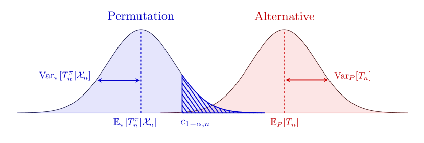
Figure 2: An illustration of Lemma 3.1. The lemma describes that the major components that determine the power of a permutation test are the mean and the variance of the alternative distribution as well as the permutation distribution. In particular, if the mean of the alternative distribution is sufficiently larger than the other components (on average since the permutation distribution is random), then the permutation test succeeds to reject the null with high probability.

4 The two moments method for two-sample testing

This section illustrates the two moments method given in Lemma 3.1 for two-sample testing. By focusing on a $U$-statistic, we first present a general condition that ensures that the type I and II error rates of the permutation test are uniformly controlled (Theorem 4.1). We then turn to more specific cases of two-sample testing for multinomial distributions and Hölder densities.

Let $g(x,y)$ be a bivariate function, which is symmetric in its arguments, i.e. $g(x,y)=g(y,x)$. Based on this bivariate function, let us define a kernel for a two-sample $U$-statistic

$$h_{\text{ts}}(y_{1},y_{2};z_{1},z_{2}):=g(y_{1},y_{2})+g(z_{1},z_{2})-g(y_{1},z_{2})-g(y_{2},z_{1}),$$ (5)

and write the corresponding $U$-statistic as

$$U_{n_{1},n_{2}}:=\frac{1}{(n_{1})_{(2)}(n_{2})_{(2)}}\sum_{(i_{1},i_{2})\in\mathbf{i}_{2}^{n_{1}}}\sum_{(j_{1},j_{2})\in\mathbf{i}_{2}^{n_{2}}}h_{\text{ts}}(Y_{i_{1}},Y_{i_{2}};Z_{j_{1}},Z_{j_{2}}).$$ (6)

Depending on the choice of kernel $h_{\text{ts}}$, the $U$-statistic includes frequently used two-sample test statistics in the literature such as the maximum mean discrepancy (Gretton et al.,, 2012) and the energy statistic (Baringhaus and Franz,, 2004; Székely and Rizzo,, 2004). From the basic properties of $U$-statistics (e.g. Lee,, 1990), it is readily seen that $U_{n_{1},n_{2}}$ is an unbiased estimator of $\mathbb{E}_{P}[h_{\text{ts}}(Y_{1},Y_{2};Z_{1},Z_{2})]$. To describe the main result of this section, let us write the symmetrized kernel by

$$\overline{h}_{\text{ts}}(y_{1},y_{2};z_{1},z_{2}):=\frac{1}{2!2!}\sum_{(i_{1},i_{2})\in\mathbf{i}_{2}^{2}}\sum_{(j_{1},j_{2})\in\mathbf{i}_{2}^{2}}h_{\text{ts}}(y_{i_{1}},y_{i_{2}};z_{j_{1}},z_{j_{2}}),$$ (7)

and define $\psi_{Y,1}(P),\psi_{Z,1}(P)$ and $\psi_{YZ,2}(P)$ by

$$\psi_{Y,1}(P) :=\text{Var}_{P}[\mathbb{E}_{P}\{\overline{h}_{\text{ts}}(Y_{1},Y_{2};Z_{1},Z_{2})|Y_{1}\}],$$ (8)

$$\psi_{Z,1}(P) :=\text{Var}_{P}[\mathbb{E}_{P}\{\overline{h}_{\text{ts}}(Y_{1},Y_{2};Z_{1},Z_{2})|Z_{1}\}],$$

$$\psi_{YZ,2}(P) :=\max\{\mathbb{E}_{P}[g^{2}(Y_{1},Y_{2})],\ \mathbb{E}_{P}[g^{2}(Y_{1},Z_{1})],\ \mathbb{E}_{P}[g^{2}(Z_{1},Z_{2})]\}.$$

As will be clearer in the sequel $\psi_{Y,1}(P),\psi_{Z,1}(P)$ and $\psi_{YZ,2}(P)$ are key quantities which we use to upper bound the variance of $U_{n_{1},n_{2}}$. By leveraging Lemma 3.1, the next theorem presents a sufficient condition that guarantees that the type II error rate of the permutation test based on $U_{n_{1},n_{2}}$ is uniformly bounded by $\beta$.

Theorem 4.1 (Two-sample $U$-statistic).

Suppose that there is a sufficiently large constant $C>0$ such that

$$\mathbb{E}_{P}[U_{n_{1},n_{2}}]\geq C\sqrt{\max\Bigg{\{}\frac{\psi_{Y,1}(P)}{\beta n_{1}},\ \frac{\psi_{Z,1}(P)}{\beta n_{2}},\ \frac{\psi_{YZ,2}(P)}{\alpha\beta}\left(\frac{1}{n_{1}}+\frac{1}{n_{2}}\right)^{2}\Bigg{\}}},$$ (9)

for all $P\in\mathcal{P}_{1}$. Then the type II error of the permutation test over $\mathcal{P}_{1}$ is uniformly bounded by $\beta$, that is

$$\sup_{P\in\mathcal{P}_{1}}\mathbb{P}_{P}^{(n_{1},n_{2})}(U_{n_{1},n_{2}}\leq c_{1-\alpha,n_{1},n_{2}})\leq\beta.$$

Remark 4.2.

• This result, applicable broadly to degenerate $U$-statistics of the form in (6), simplifies the application of Lemma 3.1. The main difficulty in directly applying Lemma 3.1 is that the sufficient condition depends on the conditional variance of the statistic under the permutation distribution which can be challenging to upper bound. On the other hand the sufficient condition of this theorem, only depends on the quantities in (8) which do not depend on the permutation distribution.

• The main technical effort in establishing this result is in showing (11), which upper bounds the conditional variance of the test statistic under the permutation distribution, as a function of the quantity $\psi_{YZ,2}(P)$ defined in (8).

• In Theorem 4.1 and other places, we say that $C$ is a universal constant when it does not depend on other quantities. When the constant is not universal but depends on problem-specific quantities (say $\theta_{1},\theta_{2},\ldots$), which are typically considered fixed (for instance, density smoothness parameters in non-parametric testing), we denote this via the explicit notation $C(\theta_{1},\theta_{2},\ldots)$. Importantly, these constants do not depend on the sample-size.

Proof Sketch..

Let us give a high-level idea of the proof, while the details are deferred to Appendix F. First, by the linearity of expectation, it can be verified that the mean of the permuted $U$-statistic $U_{n_{1},n_{2}}^{\pi}$ is zero. Therefore it suffices to check condition (4). By the well-known variance formula of a two-sample $U$-statistic (e.g. page 38 of Lee,, 1990), we prove in Appendix F that

$$\text{Var}_{P}[U_{n_{1},n_{2}}]\leq C_{1}\frac{\psi_{Y,1}(P)}{n_{1}}+C_{2}\frac{\psi_{Z,1}(P)}{n_{2}}+C_{3}\psi_{YZ,2}(P)\left(\frac{1}{n_{1}}+\frac{1}{n_{2}}\right)^{2},$$ (10)

and this result can be used to bound the first term of condition (4). It is worth pointing out that the variance behaves differently under the null and alternative hypotheses. In particular, $\psi_{Y,1}$ and $\psi_{Z,1}$ are zero under the null hypothesis. Hence, in the null case, the third term dominates the variance of $U_{n_{1},n_{2}}$ where we note that $\psi_{YZ,2}$ is a convenient upper bound for the variance of kernel $h_{\text{ts}}$. Intuitively, the permuted $U$-statistic $U_{n_{1},n_{2}}^{\pi}$ behaves similarly to $U_{n_{1},n_{2}}$ computed based on samples from a certain null distribution (say a mixture of $P_{Y}$ and $P_{Z}$). This implies that the variance of $U_{n_{1},n_{2}}^{\pi}$ is also dominated by the third term in the upper bound (10). Having this intuition in mind, we use the symmetric structure of kernel $h_{\text{ts}}$ and prove that

$$\mathbb{E}_{P}[\text{Var}_{\pi}\{T_{n}^{\pi}|\mathcal{X}_{n}\}]\leq C_{4}\psi_{YZ,2}(P)\left(\frac{1}{n_{1}}+\frac{1}{n_{2}}\right)^{2},$$ (11)

which is one of our key technical contributions. Based on the previous two bounds in (10) and (11), we then complete the proof by verifying the sufficient condition (4). ∎

The next two subsections focus on multinomial distributions and Hölder densities and give explicit expressions for condition (9). We also demonstrate minimax optimality of permutation tests under the given scenarios.

4.1 Two-sample testing for multinomials

Let $p_{Y}$ and $p_{Z}$ be multinomial distributions on a discrete domain $\mathbb{S}_{d}:=\{1,\ldots,d\}$. Throughout this subsection, we consider the kernel $h_{\text{ts}}(y_{1},y_{2};z_{1},z_{2})$ in (5) defined with the following bivariate function:

$$g_{\text{Multi}}(x,y):=\sum_{k=1}^{d}\mathds{1}(x=k)\mathds{1}(y=k).$$ (12)

It is straightforward to see that the resulting $U$-statistic (6) is an unbiased estimator of $\|p_{Y}-p_{Z}\|_{2}^{2}$. Let us denote the maximum between the squared $\ell_{2}$ norms of $p_{Y}$ and $p_{Z}$ by

$$b_{(1)}:=\max\big{\{}\|p_{Y}\|_{2}^{2},\|p_{Z}\|_{2}^{2}\big{\}}.$$ (13)

Building on Theorem 4.1, the next result establishes a guarantee on the testing errors of the permutation test under the two-sample multinomial setting.

Proposition 4.3 (Multinomial two-sample testing in $\ell_{2}$ distance).

Let $\mathcal{P}_{\text{\emph{Multi}}}^{(d)}$ be the set of pairs of multinomial distributions defined on $\mathbb{S}_{d}$. Let $\mathcal{P}_{0}=\{(p_{Y},p_{Z})\in\mathcal{P}_{\text{\emph{Multi}}}^{(d)}:p_{Y}=p_{Z}\}$ and $\mathcal{P}_{1}(\epsilon_{n_{1},n_{2}})=\{(p_{Y},p_{Z})\in\mathcal{P}_{\text{\emph{Multi}}}^{(d)}:\|p_{Y}-p_{Z}\|_{2}\geq\epsilon_{n_{1},n_{2}}\}$ where

$$\epsilon_{n_{1},n_{2}}\geq C\frac{b_{(1)}^{1/4}}{\alpha^{1/4}\beta^{1/2}}\left(\frac{1}{n_{1}}+\frac{1}{n_{2}}\right)^{1/2},$$

for a sufficiently large $C>0$. Consider the two-sample $U$-statistic $U_{n_{1},n_{2}}$ defined with the bivariate function $g_{\text{\emph{Multi}}}$ given in (12). Then the type I and II error rates of the resulting permutation test are uniformly bounded over the classes $\mathcal{P}_{0}$ and $\mathcal{P}_{1}$ as in (LABEL:Eq:_uniform_error_control).

Proof Sketch..

We outline the proof of the result, while the details can be found in Appendix G. Given the reduction in Theorem 4.1 the remaining technical effort is to show that there exist constants $C_{1},C_{2},C_{3}>0$ such that

$$\psi_{Y,1}(P) \leq C_{1}\sqrt{b_{(1)}}\|p_{Y}-p_{Z}\|_{2}^{2},$$ (14)

$$\psi_{Z,1}(P) \leq C_{2}\sqrt{b_{(1)}}\|p_{Y}-p_{Z}\|_{2}^{2},$$

$$\psi_{YZ,2}(P) \leq C_{3}b_{(1)}.$$

We note that the U-statistic with kernel in (12) is similar (although not identical) to the statistic proposed by Chan et al., (2014) for the case when the sample-sizes are equal, and they derive similar bounds on the variance of their test statistic. These bounds together with Theorem 4.1 imply that if there exists a sufficiently large $C_{4}>0$ such that

$$\|p_{Y}-p_{Z}\|_{2}^{2}\geq C_{4}\frac{\sqrt{b_{(1)}}}{\alpha^{1/2}\beta}\left(\frac{1}{n_{1}}+\frac{1}{n_{2}}\right),$$ (15)

then the permutation test based on $U_{n_{1},n_{2}}$ has non-trivial power as claimed. ∎

For the balanced case where $n_{1}=n_{2}$, Chan et al., (2014) prove that no test can have uniform power if $\epsilon_{n_{1},n_{2}}$ is of lower order than $b_{(1)}^{1/4}n_{1}^{-1/2}$. Hence the permutation test in Proposition 4.3 is minimax rate optimal in this balanced setting. The next proposition extends this result to the case of unequal sample sizes and shows that the permutation test is still optimal even for the unbalanced case.

Proposition 4.4 (Minimum separation for two-sample multinomial testing).

Consider the two-sample testing problem within the class of multinomial distributions $\mathcal{P}_{\text{\emph{Multi}}}^{(d)}$ where the null hypothesis and the alternative hypothesis are $H_{0}:p_{Y}=p_{Z}$ and $H_{1}:\|p_{Y}-p_{Z}\|_{2}\geq\epsilon_{n_{1},n_{2}}$. Under this setting and $n_{1}\leq n_{2}$, the minimum separation satisfies $\epsilon_{n_{1},n_{2}}^{\dagger}\asymp b_{(1)}^{1/4}n_{1}^{-1/2}$.

Remark 4.5 ($\ell_{1}$- versus $\ell_{2}$-closeness testing).

We note that the minimum separation strongly depends on the choice of metrics. As shown in Bhattacharya and Valiant, (2015) and Diakonikolas and Kane, (2016), the minimum separation rate for two-sample testing in the $\ell_{1}$ distance is $\max\{d^{1/2}n_{2}^{-1/4}n_{1}^{-1/2},d^{1/4}n_{1}^{-1/2}\}$ for $n_{1}\leq n_{2}$. This rate, in contrast to $b_{(1)}^{1/4}n_{1}^{-1/2}$, illustrates that the difficulty of $\ell_{1}$-closeness testing depends not only on the smaller sample size $n_{1}$ but also on the larger sample size $n_{2}$. In Section 8.2, we provide a permutation test that is minimax rate optimal in the $\ell_{1}$ distance.

Proof Sketch..

We prove Proposition 4.4 indirectly by finding the minimum separation for one-sample multinomial testing. The goal of the one-sample problem is to test whether one set of samples is drawn from a known multinomial distribution. Intuitively the one-sample problem is no harder than the two-sample problem as the former can always be transformed into the latter by drawing another set of samples from the known distribution. This intuition was formalized by Arias-Castro et al., (2018) in which they showed that the minimax risk of the one-sample problem is no larger than that of the two-sample problem (see their Lemma 1). We prove in Appendix H that the minimum separation for the one-sample problem is of order $b_{(1)}^{1/4}n_{1}^{-1/2}$ and it thus follows that $b_{(1)}^{1/4}n_{1}^{-1/2}\lesssim\epsilon_{n_{1},n_{2}}^{\dagger}$. The proof is completed by comparing this lower bound with the upper bound established in Proposition 4.3. ∎

4.2 Two-sample testing for Hölder densities

We next focus on testing for the equality between two density functions under Hölder’s regularity condition. Adopting the notation used in Arias-Castro et al., (2018), let $\mathcal{H}^{d}_{s}(L)$ be the class of functions $f:[0,1]^{d}\mapsto\mathbb{R}$ such that

1. $\big{|}f^{(\lfloor s\rfloor)}(x)-f^{(\lfloor s\rfloor)}(x^{\prime})\big{|}\leq L\|x-x^{\prime}\|^{s-\lfloor s\rfloor},\quad\forall x,x^{\prime}\in[0,1]^{d},$

2. $|\!|\!|f^{(s^{\prime})}|\!|\!|_{\infty}\leq L$ for each $s^{\prime}\in\{1,\ldots,\lfloor s\rfloor\}$,

where $f^{(\lfloor s\rfloor)}$ denotes the $\lfloor s\rfloor$-order derivative of $f$. Let us write the $L_{2}$ norm of $f\in\mathcal{H}^{d}_{s}(L)$ by $|\!|\!|f|\!|\!|_{L_{2}}^{2}:=\int f^{2}(x)dx$. By letting $f_{Y}$ and $f_{Z}$ be the density functions of $P_{Y}$ and $P_{Z}$ with respect to Lebesgue measure, we define the set of $(P_{Y},P_{Z})$, denoted by $\mathcal{P}_{\text{{H\"{o}lder}}}^{(d,s)}$, such that both $f_{Y}$ and $f_{Z}$ belong to $\mathcal{H}^{d}_{s}(L)$. For this Hölder density class $\mathcal{P}_{\text{{H\"{o}lder}}}^{(d,s)}$ and $n_{1}\leq n_{2}$, Arias-Castro et al., (2018) establish that for testing $H_{0}:f_{Y}=f_{Z}$ against $H_{1}:|\!|\!|f_{Y}-f_{Z}|\!|\!|_{L_{2}}\geq\epsilon_{n_{1},n_{2}}$, the minimum separation rate satisfies

$$\epsilon_{n_{1},n_{2}}^{\dagger}\asymp n_{1}^{-2s/(4s+d)}.$$ (16)

We note that this optimal testing rate is faster than the $n^{-s/(2s+d)}$ rate for estimating a Hölder density in the $L_{2}$ loss (see for instance Tsybakov,, 2009). It is further shown in Arias-Castro et al., (2018) that the optimal rate (16) is achieved by the unnormalized chi-square test but with a somewhat loose threshold. Although they recommend a critical value calibrated by permutation in practice, it is unknown whether the resulting test has the same theoretical guarantees. We also note that their testing procedure discards $n_{2}-n_{1}$ observations to balance the sample sizes, which may lead to a less powerful test in practice. Motivated by these limitations, we propose an alternative test for Hölder densities, building on the multinomial permutation test in Proposition 4.3.

To implement the multinomial test for continuous data, we first need to discretize the support $[0,1]^{d}$. We follow the same strategy as in, for instance, Ingster, (1987); Arias-Castro et al., (2018); Balakrishnan and Wasserman, (2019) and consider bins of equal sizes that partition $[0,1]^{d}$. These bins are $d$-dimensional hypercubes whose length is set to $\kappa_{(1)}^{-1}$ where

$$\kappa_{(1)}:=\lfloor n_{1}^{2/(4s+d)}\rfloor.$$

Let $\{B_{1},\ldots,B_{K}\}$ be an enumeration of such hypercubes. Next, consider a discretization function $Q:[0,1]^{p}\mapsto\{1,\ldots,K\}$ such that $Q(x)=k$ if and only if $x\in B_{k}$. Then, based on the discretized data $\{Q(Y_{1}),\ldots,Q(Y_{n_{1}})\}$ and $\{Q(Z_{1}),\ldots,Q(Z_{n_{2}})\}$, we can now apply the multinomial test in Proposition 4.3 and the resulting test has the following theoretical guarantees for density testing.

Proposition 4.6 (Two-sample testing for Hölder densities).

Consider the multinomial test considered in Proposition 4.3 based on the equal-sized binned data described above. For a sufficiently large $C(s,d,L)>0$, consider $\epsilon_{n_{1},n_{2}}$ such that

$$\epsilon_{n_{1},n_{2}}\geq\frac{C(s,d,L)}{\alpha^{1/4}\beta^{1/2}}\left(\frac{1}{n_{1}}+\frac{1}{n_{2}}\right)^{\frac{2s}{4s+d}}.$$

Then for testing $\mathcal{P}_{0}=\{(P_{Y},P_{Z})\in\mathcal{P}_{\text{\emph{H\"{o}lder}}}^{(d,s)}:f_{Y}=f_{Z}\}$ against $\mathcal{P}_{1}=\{(P_{Y},P_{Z})\in\mathcal{P}_{\text{\emph{H\"{o}lder}}}^{(d,s)}:|\!|\!|f_{Y}-f_{Z}|\!|\!|_{L_{2}}\geq\epsilon_{n_{1},n_{2}}\}$, the type I and II error rates of the resulting permutation test are uniformly controlled as in (LABEL:Eq:_uniform_error_control).

The proof of this result uses Proposition 4.3 along with careful analysis of the approximation errors from discretization, building on the analysis of Ingster, (2000); Arias-Castro et al., (2018). The details can be found in Appendix I. We remark that type I error control of the multinomial test follows clearly by the permutation principle, which is not affected by discretization. From the minimum separation rate given in (16), it is clear that the proposed test is minimax rate optimal for two-sample testing within Hölder class and it works for both equal and unequal sample sizes without discarding the data. However it is also important to note that the proposed test as well as the test introduced by Arias-Castro et al., (2018) depend on knowledge of the smoothness parameter $s$, which is perhaps unrealistic in practice. To address this issue, Arias-Castro et al., (2018) build upon the work of Ingster, (2000) and propose a Bonferroni-type testing procedure that adapts to this unknown parameter at the cost of a $\log n$ factor. In Section 7, we improve this logarithmic cost to an iterated logarithmic factor, leveraging combinatorial concentration inequalities developed in Section 6.

5 The two moments method for independence testing

In this section we present analogous results to those in Section 4 for independence testing. We start by introducing a $U$-statistic for independence testing and establish a general condition under which the permutation test based on the $U$-statistic controls the type I and II error rates (Theorem 5.1). We then move on to more specific cases of testing for multinomials and Hölder densities in Section 5.1 and Section 5.2, respectively.

Let us consider two bivariate functions $g_{Y}(y_{1},y_{2})$ and $g_{Z}(z_{1},z_{2})$, which are symmetric in their arguments. Define a product kernel associated with $g_{Y}(y_{1},y_{2})$ and $g_{Z}(z_{1},z_{2})$ by

$$h_{\text{in}}\{(y_{1},z_{1}),(y_{2},z_{2}),(y_{3},z_{3}),(y_{4},z_{4})\}:=\big{\{}g_{Y}(y_{1},y_{2})+g_{Y}(y_{3},y_{4})$$ (17)

$$- g_{Y}(y_{1},y_{3})-g_{Y}(y_{2},y_{4})\big{\}}\cdot\big{\{}g_{Z}(z_{1},z_{2})+g_{Z}(z_{3},z_{4})-g_{Z}(z_{1},z_{3})-g_{Z}(z_{2},z_{4})\big{\}}.$$

For simplicity, we may also write $h_{\text{in}}\{(y_{1},z_{1}),(y_{2},z_{2}),(y_{3},z_{3}),(y_{4},z_{4})\}$ as $h_{\text{in}}(x_{1},x_{2},x_{3},x_{4})$. Given this fourth order kernel, consider a $U$-statistic defined by

$$U_{n}:=\frac{1}{n_{(4)}}\sum_{(i_{1},i_{2},i_{3},i_{4})\in\mathbf{i}_{4}^{n}}h_{\text{in}}(X_{i_{1}},X_{i_{2}},X_{i_{3}},X_{i_{4}}).$$ (18)

Again, by the unbiasedness property of $U$-statistics (e.g. Lee,, 1990), it is clear that $U_{n}$ is an unbiased estimator of $\mathbb{E}_{P}[h_{\text{in}}(X_{1},X_{2},X_{3},X_{4})]$. Depending on the choice of kernel $h_{\text{in}}$, the considered $U$-statistic covers numerous test statistics for independence testing including the Hilbert–Schmidt Independence Criterion (HSIC) (Gretton et al.,, 2005) and distance covariance (Székely et al.,, 2007). Let $\overline{h}_{\text{in}}(x_{1},x_{2},x_{3},x_{4})$ be the symmetrized version of $h_{\text{in}}(x_{1},x_{2},x_{3},x_{4})$ given by

$$\overline{h}_{\text{in}}(x_{1},x_{2},x_{3},x_{4}):=\frac{1}{4!}\sum_{(i_{1},i_{2},i_{3},i_{4})\in\mathbf{i}_{4}^{4}}h_{\text{in}}(x_{i_{1}},x_{i_{2}},x_{i_{3}},x_{i_{4}}).$$

In a similar fashion to $\psi_{Y,1}(P),\psi_{Z,1}(P)$ and $\psi_{YZ,2}(P)$, we define $\psi_{1}^{\prime}(P)$ and $\psi_{2}^{\prime}(P)$ by

$$\psi_{1}^{\prime}(P) :=\text{Var}_{P}[\mathbb{E}_{P}\{\overline{h}_{\text{in}}(X_{1},X_{2},X_{3},X_{4})|X_{1}\}],$$ (19)

$$\psi_{2}^{\prime}(P) :=\max\big{\{}\mathbb{E}_{P}[g_{Y}^{2}(Y_{1},Y_{2})g_{Z}^{2}(Z_{1},Z_{2})],\ \mathbb{E}_{P}[g_{Y}^{2}(Y_{1},Y_{2})g_{Z}^{2}(Z_{1},Z_{3})],$$

$$~{}~{}~{}~{}~{}~{}~{}~{}~{}~{}~{}~{}~{}\mathbb{E}_{P}[g_{Y}^{2}(Y_{1},Y_{2})g_{Z}^{2}(Z_{3},Z_{4})]\big{\}}.$$

The following theorem studies the type II error of the permutation test based on $U_{n}$.

Theorem 5.1 ($U$-statistic for independence testing).

Suppose that there is a sufficiently large constant $C>0$ such that

$$\mathbb{E}_{P}[U_{n}]\geq C\sqrt{\max\Bigg{\{}\frac{\psi_{1}^{\prime}(P)}{\beta n},\ \frac{\psi_{2}^{\prime}(P)}{\alpha\beta n^{2}}\Bigg{\}}},$$

for all $P\in\mathcal{P}_{1}$. Then the type II error of the permutation test over $\mathcal{P}_{1}$ is uniformly bounded by $\beta$, that is

$$\sup_{P\in\mathcal{P}_{1}}\mathbb{P}_{P}^{(n)}(U_{n}\leq c_{1-\alpha,n})\leq\beta.$$

Remark 5.2.

Analogous to Theorem 4.1, for degenerate U-statistics of the form (18), this result simplifies the application of Lemma 3.1 by reducing the sufficient condition to only depend on the quantities in (19). Importantly, these quantities do not depend on the permutation distribution of the test statistic.

Proof Sketch..

The proof of Theorem 5.1 proceeds similarly as the proof of Theorem 4.1. Here we present a brief overview of the proof, while the details can be found in Appendix J. First of all, the permuted $U$-statistic $U_{n}^{\pi}$ is centered and it suffices to verify the simplified condition (4). To this end, based on the explicit variance formula of a $U$-statistic (e.g. page 12 of Lee,, 1990), we prove that

$$\text{Var}_{P}[U_{n}]\leq C_{1}\frac{\psi_{1}^{\prime}(P)}{n}+C_{2}\frac{\psi_{2}^{\prime}(P)}{n^{2}}.$$ (20)

Analogous to the case of the two-sample $U$-statistic, the variance of $U_{n}$ behaves differently under the null and alternative hypotheses. In particular, under the null hypothesis, $\psi_{1}^{\prime}(P)$ becomes zero and thus the second term dominates the upper bound (20). Since the permuted $U$-statistic $U_{n}^{\pi}$ mimics the behavior of $U_{n}$ under the null, the variance of $U_{n}^{\pi}$ is expected to be similarly bounded. We make this statement precise by proving the following result:

$$\mathbb{E}_{P}[\text{Var}_{\pi}\{U_{n}^{\pi}|\mathcal{X}_{n}\}]\leq C_{3}\frac{\psi_{2}^{\prime}(P)}{n^{2}}.$$ (21)

Again, this part of the proof heavily relies on the symmetric structure of kernel $h_{\text{in}}$ and the details are deferred to Appendix J. Now by combining the established bounds (20) and (21) together with the sufficient condition (4), we can conclude Theorem 5.1. ∎

In the following subsections, we illustrate Theorem 5.1 in the context of testing multinomial distributions and Hölder densities.

5.1 Independence testing for multinomials

We begin with the case of multinomial distributions. Let $p_{YZ}$ denote a multinomial distribution on a product domain $\mathbb{S}_{d_{1},d_{2}}:=\{1,\ldots,d_{1}\}\times\{1,\ldots,d_{2}\}$ and $p_{Y}$ and $p_{Z}$ be its marginal distributions. Let us recall the kernel $h_{\text{in}}(x_{1},x_{2},x_{3},x_{4})$ in (LABEL:Eq:_Independence_kernel) and define it with the following bivariate functions:

$$g_{\text{Multi},Y}(y_{1},y_{2}):=\sum_{k=1}^{d_{1}}\mathds{1}(y_{1}=k)\mathds{1}(y_{2}=k)\quad\text{and}$$ (22)

$$g_{\text{Multi},Z}(z_{1},z_{2}):=\sum_{k=1}^{d_{2}}\mathds{1}(z_{1}=k)\mathds{1}(z_{2}=k).$$

In this case, the expectation of the $U$-statistic is $4\|p_{YZ}-p_{Y}p_{Z}\|_{2}^{2}$. Analogous to the term $b_{(1)}$ in the two-sample case, let us define

$$b_{(2)}:=\max\big{\{}\|p_{YZ}\|_{2}^{2},\|p_{Y}p_{Z}\|_{2}^{2}\big{\}}.$$ (23)

Building on Theorem 5.1, the next result establishes a guarantee on the testing errors of the permutation test for multinomial independence testing.

Proposition 5.3 (Multinomial independence testing in $\ell_{2}$ distance).

Let $\mathcal{P}_{\text{\emph{Multi}}}^{(d_{1},d_{2})}$ be the set of multinomial distributions defined on $\mathbb{S}_{d_{1},d_{2}}$. Let $\mathcal{P}_{0}=\{p_{YZ}\in\mathcal{P}_{\text{\emph{Multi}}}^{(d_{1},d_{2})}:p_{YZ}=p_{Y}p_{Z}\}$ and $\mathcal{P}_{1}(\epsilon_{n})=\{p_{YZ}\in\mathcal{P}_{\text{\emph{Multi}}}^{(d_{1},d_{2})}:\|p_{YZ}-p_{Y}p_{Z}\|_{2}\geq\epsilon_{n}\}$ where

$$\epsilon_{n}\geq\frac{C}{\alpha^{1/4}\beta^{1/2}}\frac{b_{(2)}^{1/4}}{n^{1/2}},$$

for a sufficiently large $C>0$. Consider the $U$-statistic $U_{n}$ in (18) defined with the bivariate functions $g_{\text{\emph{Multi}},Y}$ and $g_{\text{\emph{Multi}},Z}$ given in (LABEL:Eq:_Independence_bivariate_functions). Then, over the classes $\mathcal{P}_{0}$ and $\mathcal{P}_{1}$, the type I and II errors of the resulting permutation test are uniformly bounded as in (LABEL:Eq:_uniform_error_control).

Proof Sketch..

We outline the proof of the result, while the details can be found in Appendix K. In the proof, we prove that there exist constants $C_{1},C_{2}>0$ such that

$$\psi_{1}^{\prime}(P)\leq C_{1}\sqrt{b_{(2)}}\|p_{YZ}-p_{Y}p_{Z}\|_{2}^{2},$$ (24)

$$\psi_{2}^{\prime}(P)\leq C_{2}b_{(2)}.$$

These bounds combined with Theorem 5.1 yields that if there exists a sufficiently large $C_{3}>0$ such that

$$\|p_{YZ}-p_{Y}p_{Z}\|_{2}^{2}\geq\frac{C_{3}}{\alpha^{1/2}\beta}\frac{\sqrt{b_{(2)}}}{n},$$ (25)

then the type II error of the permutation test can be controlled by $\beta$ as desired. ∎

The next proposition asserts that the minimum separation rate for independence testing in the $\ell_{2}$ distance is $\epsilon_{n}^{\dagger}\asymp b_{(2)}^{1/4}n^{-1/2}$. This implies that the permutation test based on $U_{n}$ in Proposition 5.3 is minimax rate optimal in this scenario.

Proposition 5.4 (Minimum separation for multinomial independence testing).

Consider the independence testing problem within the class of multinomial distributions $\mathcal{P}_{\text{\emph{Multi}}}^{(d_{1},d_{2})}$ where the null hypothesis and the alternative hypothesis are $H_{0}:p_{YZ}=p_{Y}p_{Z}$ and $H_{1}:\|p_{YZ}-p_{Y}p_{Z}\|_{2}\geq\epsilon_{n}$. Under this setting, the minimum separation satisfies $\epsilon_{n}^{\dagger}\asymp b_{(2)}^{1/4}n^{-1/2}$.

The proof of Proposition 5.4 is based on the standard lower bound technique of Ingster, (1987) using a uniform mixture of alternative distributions. However, we remark that care is needed in order to ensure that alternative distributions are proper (normalized) multinomial distributions. To this end, we carefully perturb the uniform null distribution to generate a mixture of dependent alternative distributions, and use the property of negative association to deal with the dependency induced in ensuring the resulting distributions are normalized. The details can be found in Appendix L. In the next subsection, we turn our attention to the class of Hölder densities and provide similar results of Section 4.2 for independence testing.

5.2 Independence testing for Hölder densities

Turning to the case of Hölder densities, we leverage the previous multinomial result and establish the minimax rate for independence testing under the Hölder’s regularity condition. As in Section 4.2, we restrict our attention to functions $f:[0,1]^{d_{1}+d_{2}}\mapsto\mathbb{R}$ that satisfy

1. $\big{|}f^{(\lfloor s\rfloor)}(x)-f^{(\lfloor s\rfloor)}(x^{\prime})\big{|}\leq L\|x-x^{\prime}\|^{s-\lfloor s\rfloor},\quad\forall x,x^{\prime}\in[0,1]^{d_{1}+d_{2}},$

2. $|\!|\!|f^{(s^{\prime})}|\!|\!|_{\infty}\leq L$ for each $s^{\prime}\in\{1,\ldots,\lfloor s\rfloor\}$.

Let us write $\mathcal{H}_{s}^{d_{1}+d_{2}}(L)$ to denote the class of such functions. We further introduce the class of joint distributions, denoted by $\mathcal{P}_{\text{H\"{o}lder}}^{(d_{1}+d_{2},s)}$, defined as follows. Let $f_{YZ}$ and $f_{Y}f_{Z}$ be the densities of $P_{YZ}$ and $P_{Y}P_{Z}$ with respect to Lebesgue measure. Then $\mathcal{P}_{\text{{H\"{o}lder}}}^{(d_{1}+d_{2},s)}$ is defined as the set of joint distributions $P_{YZ}$ such that both the joint density and the product density, $f_{YZ}$ and $f_{Y}f_{Z}$, belong to $\mathcal{H}^{d_{1}+d_{2}}_{s}(L)$. Consider partitions of $[0,1]^{d_{1}+d_{2}}$ into bins of equal size and set the bin size to be $\kappa_{(2)}^{-1}$ where $\kappa_{(2)}=\lfloor n^{2/(4s+d_{1}+d_{2})}\rfloor$. Based on these equal-sized partitions, one may apply the multinomial test for independence provided in Proposition 5.3. Despite discretization, the resulting test has valid level $\alpha$ due to the permutation principle and has the following theoretical guarantees for density testing over $\mathcal{P}_{\text{{H\"{o}lder}}}^{(d_{1}+d_{2},s)}$.

Proposition 5.5 (Independence testing for Hölder densities).

Consider the multinomial independence test considered in Proposition 5.3 based on the binned data described above. For a sufficiently large $C(s,d_{1},d_{2},L)>0$, consider $\epsilon_{n}$ defined by

$$\epsilon_{n}\geq\frac{C(s,d_{1},d_{2},L)}{\alpha^{1/4}\beta^{1/2}}\left(\frac{1}{n}\right)^{\frac{2s}{4s+d_{1}+d_{2}}}.$$

Then for testing $\mathcal{P}_{0}=\{P_{YZ}\in\mathcal{P}_{\text{\emph{H\"{o}lder}}}^{(d_{1}+d_{2},s)}:f_{YZ}=f_{Y}f_{Z}\}$ against $\mathcal{P}_{1}=\{P_{YZ}\in\mathcal{P}_{\text{\emph{H\"{o}lder}}}^{(d_{1}+d_{2},s)}:|\!|\!|f_{YZ}-f_{Y}f_{Z}|\!|\!|_{L_{2}}\geq\epsilon_{n}\}$, the type I and II errors of the resulting permutation test are uniformly controlled as in (LABEL:Eq:_uniform_error_control).

The proof of the above result follows similarly to the proof of Proposition 4.6 and can be found in Appendix M. Indeed, as shown in the next proposition, the proposed binning-based independence test is minimax rate optimal for the Hölder class density functions. That is, no test can have uniform power when the separation rate $\epsilon_{n}$ is of order smaller than $n^{-2s/(4s+d_{1}+d_{2})}$.

Proposition 5.6 (Minimum separation for independence testing in Hölder class).

Consider the independence testing problem within the class $\mathcal{P}_{\text{\emph{H\"{o}lder}}}^{(d_{1}+d_{2},s)}$ in which the null hypothesis and the alternative hypothesis are $H_{0}:f_{YZ}=f_{Y}f_{Z}$ and $H_{1}:|\!|\!|f_{YZ}-f_{Y}f_{Z}|\!|\!|_{L_{2}}\geq\epsilon_{n}$. Under this setting, the minimum separation satisfies $\epsilon_{n}^{\dagger}\asymp n^{-2s/(4s+d_{1}+d_{2})}$.

The proof of Proposition 5.6 is again based on the standard lower bound technique by Ingster, (1987) and deferred to Appendix N. We note that the independence test in Proposition 5.5 hinges on the assumption that the smoothness parameter $s$ is known. To avoid this assumption, we introduce an adaptive test to this smoothness parameter at the cost of $\log\log n$ factor in Section 7. A building block for this adaptive result is combinatorial concentration inequalities developed in the next section.

6 Combinatorial concentration inequalities

Although the two moments method is broadly applicable, it may not yield sharp results when an extremely small significance level $\alpha$ is of interest (say, $\alpha$ shrinks to zero as $n$ increases). In particular, the sufficient condition (3) given by the two moments method has a polynomial dependency on $\alpha$. In this section, we develop exponential concentration inequalities for permuted $U$-statistics that allow us to improve this polynomial dependency. To this end, we introduce a novel strategy to couple a permuted $U$-statistic with i.i.d. Bernoulli or Rademacher random variables, inspired by the symmetrization trick (Duembgen,, 1998) and Hoeffding’s average (Hoeffding,, 1963).

Coupling with i.i.d. random variables. The core idea of our approach is fairly general and based on the following simple observation. Given a random permutation $\pi$ uniformly distributed over $\mathbf{\Pi}_{n}$, we randomly switch the order within $(\pi_{2i-1},\pi_{2i})$ for $i=1,2,\ldots,\lfloor n/2\rfloor$. We denote the resulting permutation by $\pi^{\prime}$. It is clear that $\pi$ and $\pi^{\prime}$ are dependent but identically distributed. The point of introducing this extra permutation $\pi^{\prime}$ is that we are now able to associate $\pi^{\prime}$ with i.i.d. Bernoulli random variables without changing the distribution. To be more specific, let $\delta_{1},\ldots,\delta_{\lfloor n/2\rfloor}$ be i.i.d. Bernoulli random variables with success probability $1/2$. Then $(\pi_{2i-1}^{\prime},\pi_{2i}^{\prime})$ can be written as

$$(\pi_{2i-1}^{\prime},\pi_{2i}^{\prime})=\big{(}\delta_{i}\pi_{2i-1}+(1-\delta_{i})\pi_{2i},(1-\delta_{i})\pi_{2i-1}+\delta_{i}\pi_{2i}\big{)}\quad\text{for $i=1,2,\ldots,\lfloor n/2\rfloor$}.$$

Given that it is easier to work with i.i.d. samples than permutations, the alternative representation of $\pi^{\prime}$ gives a nice way to investigate a general permuted statistic. The next subsections provide concrete demonstrations of this coupling approach based on degenerate $U$-statistics.

6.1 Degenerate two-sample $U$-statistics

We start with the two-sample $U$-statistic in (6). Our strategy is outlined as follows. First, motivated by Hoeffding’s average (Hoeffding,, 1963), we express the permuted $U$-statistic as the average of more tractable statistics. We then link these tractable statistics to quadratic forms of i.i.d. Rademacher random variables based on the coupling idea described before. Finally we apply existing concentration bounds for quadratic forms of i.i.d. random variables to obtain the result in Theorem 6.1.

Let us denote the permuted $U$-statistic associated with $\pi\in\mathbf{\Pi}_{n}$ by

$$U_{n_{1},n_{2}}^{\pi}:=\frac{1}{(n_{1})_{(2)}(n_{2})_{(2)}}\sum_{(i_{1},i_{2})\in\mathbf{i}_{2}^{n_{1}}}\sum_{(j_{1},j_{2})\in\mathbf{i}_{2}^{n_{2}}}h_{\text{ts}}(X_{\pi_{i_{1}}},X_{\pi_{i_{2}}};X_{\pi_{n_{1}+j_{1}}},X_{\pi_{n_{1}+j_{2}}}).$$ (26)

By assuming $n_{1}\leq n_{2}$, let $L:=\{\ell_{1},\ldots,\ell_{n_{1}}\}$ be a $n_{1}$-tuple uniformly drawn without replacement from $\{1,\ldots,n_{2}\}$. Given $L$, we introduce another test statistic

$$\widetilde{U}_{n_{1},n_{2}}^{\pi,L}:=\frac{1}{(n_{1})_{(2)}}\sum_{(k_{1},k_{2})\in\mathbf{i}_{2}^{n_{1}}}h_{\text{ts}}(X_{\pi_{k_{1}}},X_{\pi_{k_{2}}};X_{\pi_{n_{1}+\ell_{k_{1}}}},X_{\pi_{n_{1}+\ell_{k_{2}}}}).$$

By treating $L$ as a random quantity, $U_{n_{1},n_{2}}^{\pi}$ can be viewed as the expected value of $\widetilde{U}_{n_{1},n_{2}}^{\pi,L}$ with respect to $L$ (conditional on other random variables), that is,

$$U_{n_{1},n_{2}}^{\pi}=\mathbb{E}_{L}[\widetilde{U}_{n_{1},n_{2}}^{\pi,L}|\mathcal{X}_{n},\pi].$$ (27)

The idea of expressing a $U$-statistic as the average of more tractable statistics dates back to Hoeffding, (1963). The reason for introducing $\widetilde{U}_{n_{1},n_{2}}^{\pi,L}$ is to connect $U_{n_{1},n_{2}}^{\pi}$ with a Rademacher chaos. Recall that $\pi=(\pi_{1},\ldots,\pi_{n})$ is uniformly distributed over all possible permutations of $\{1,\ldots,n\}$. Therefore, as explained earlier, the distribution of $\widetilde{U}_{n_{1},n_{2}}^{\pi,L}$ does not change even if we randomly switch the order between $X_{\pi_{k}}$ and $X_{\pi_{n_{1}+\ell_{k}}}$ for $k\in\{1,\ldots,n_{1}\}$. More formally, recall that $\delta_{1},\ldots,\delta_{n_{1}}$ are i.i.d. Bernoulli random variables with success probability $1/2$. For $k=1,\ldots,n_{1}$, define

$$\widetilde{X}_{\pi_{k}}:=\delta_{k}X_{\pi_{k}}+(1-\delta_{k})X_{\pi_{n_{1}+\ell_{k}}}\quad\text{and}\quad\widetilde{X}_{\pi_{n_{1}+\ell_{k}}}:=(1-\delta_{k})X_{\pi_{k}}+\delta_{k}X_{\pi_{n_{1}+\ell_{k}}}.$$ (28)

Then it can be seen that $\widetilde{U}_{n_{1},n_{2}}^{\pi,L}$ is equal in distribution to

$$\widetilde{U}_{n_{1},n_{2}}^{\pi,L,\delta}:=\frac{1}{(n_{1})_{(2)}}\sum_{(k_{1},k_{2})\in\mathbf{i}_{2}^{n_{1}}}h_{\text{ts}}(\widetilde{X}_{\pi_{k_{1}}},\widetilde{X}_{\pi_{k_{2}}};\widetilde{X}_{\pi_{n_{1}+\ell_{k_{1}}}},\widetilde{X}_{\pi_{n_{1}+\ell_{k_{2}}}}).$$

In other words, we link $\widetilde{U}_{n_{1},n_{2}}^{\pi,L}$ to i.i.d. Bernoulli random variables, which are easier to work with. Furthermore, by the symmetry of $g(x,y)$ in its arguments and letting $\zeta_{1},\ldots,\zeta_{n}$ be i.i.d. Rademacher random variables, one can observe that $\widetilde{U}_{n_{1},n_{2}}^{\pi,L,\delta}$ is equal in distribution to the following Rademacher chaos:

$$\widetilde{U}_{n_{1},n_{2}}^{\pi,L,\zeta}:=\frac{1}{(n_{1})_{(2)}}\sum_{(k_{1},k_{2})\in\mathbf{i}_{2}^{n_{1}}}\zeta_{k_{1}}\zeta_{k_{2}}h_{\text{ts}}(X_{\pi_{k_{1}}},X_{\pi_{k_{2}}};X_{\pi_{n_{1}+\ell_{k_{1}}}},X_{\pi_{n_{1}+\ell_{k_{2}}}}).$$

Consequently, we observe that $\widetilde{U}_{n_{1},n_{2}}^{\pi,L}$ and $\widetilde{U}_{n_{1},n_{2}}^{\pi,L,\zeta}$ are equal in distribution, i.e.

$$\widetilde{U}_{n_{1},n_{2}}^{\pi,L}\overset{d}{=}\widetilde{U}_{n_{1},n_{2}}^{\pi,L,\zeta}.$$ (29)

We now have all the ingredients ready for obtaining an exponential bound for $U_{n_{1},n_{2}}^{\pi}$. By the Chernoff bound (e.g. Boucheron et al.,, 2013), for any $\lambda>0$,

$$\mathbb{P}_{\pi}\left(U_{n_{1},n_{2}}^{\pi}>t|\mathcal{X}_{n}\right)~{}\leq{} e^{-\lambda t}\mathbb{E}_{\pi}\big{[}\exp\big{(}\lambda U_{n_{1},n_{2}}^{\pi}\big{)}|\mathcal{X}_{n}\big{]}$$ (30)

$$\overset{(i)}{\leq}{} e^{-\lambda t}\mathbb{E}_{\pi,L}\big{[}\exp\big{(}\lambda\widetilde{U}_{n_{1},n_{2}}^{\pi,L}\big{)}|\mathcal{X}_{n}\big{]}$$

$$\overset{(ii)}{=}{} e^{-\lambda t}\mathbb{E}_{\pi,L,\zeta}\big{[}\exp\big{(}\lambda\widetilde{U}_{n_{1},n_{2}}^{\pi,L,\zeta}\big{)}|\mathcal{X}_{n}\big{]}$$

where step $(i)$ uses Jensen’s inequality together with (27) and step $(ii)$ holds from (29). Finally, conditional on $\pi$ and $L$, we can associate the last equation with the moment generating function of a quadratic form of i.i.d. Rademacher random variables. This quadratic form has been well-studied in the literature through a decoupling argument (e.g. Chapter 6 of Vershynin,, 2018), which leads to the following theorem. The remainder of the proof of Theorem 6.1 can be found in Section O.

Theorem 6.1 (Concentration of $U_{n_{1},n_{2}}^{\pi}$).

Consider the permuted two-sample $U$-statistic $U_{n_{1},n_{2}}^{\pi}$ (26) and define

$$\Sigma_{n_{1},n_{2}}^{2}:=\frac{1}{n_{1}^{2}(n_{1}-1)^{2}}\sup_{\pi\in\mathbf{\Pi}_{n}}\Bigg{\{}\sum_{(i_{1},i_{2})\in\mathbf{i}_{2}^{n_{1}}}g^{2}(X_{\pi_{i_{1}}},X_{\pi_{i_{2}}})\Bigg{\}}.$$

Then, for every $t>0$ and some constant $C>0$, we have

$$\mathbb{P}_{\pi}\left(U_{n_{1},n_{2}}^{\pi}\geq t~{}|\mathcal{X}_{n}\right)\leq\exp\bigg{\{}-C\min\left(\frac{t^{2}}{\Sigma_{n_{1},n_{2}}^{2}},\ \frac{t}{\Sigma_{n_{1},n_{2}}}\right)\bigg{\}}.$$

In our application, it is convenient to have an upper bound for $\Sigma_{n_{1},n_{2}}$ without involving the supremum operator. One trivial bound, suitable for our purpose, is given by

$$\Sigma_{n_{1},n_{2}}^{2}\leq\frac{1}{n_{1}^{2}(n_{1}-1)^{2}}\sum_{(i_{1},i_{2})\in\mathbf{i}_{2}^{n}}g^{2}(X_{i_{1}},X_{i_{2}}).$$ (31)

The next subsection presents an analogous result for degenerate $U$-statistics in the context of independence testing.

6.2 Degenerate $U$-statistics for independence testing

Let us recall the $U$-statistic for independence testing in (18) and denote the permuted version by

$$U_{n}^{\pi}:=\frac{1}{n_{(4)}}\sum_{(i_{1},i_{2},i_{3},i_{4})\in\mathbf{i}_{4}^{n}}h_{\text{in}}\big{\{}(Y_{i_{1}},Z_{\pi_{i_{1}}}),(Y_{i_{2}},Z_{\pi_{i_{2}}}),(Y_{i_{3}},Z_{\pi_{i_{3}}}),(Y_{i_{4}},Z_{\pi_{i_{4}}})\big{\}}.$$ (32)

We follow a similar strategy taken in the previous subsection to obtain an exponential bound for $U_{n}^{\pi}$. To this end, we first introduce some notation. Let $L:=\{\ell_{1},\ldots,\ell_{\lfloor n/2\rfloor}\}$ be a $\lfloor n/2\rfloor$-tuple uniformly sampled without replacement from $\{1,\ldots,n\}$ and similarly $L^{\prime}:=\{\ell_{1}^{\prime},\ldots,\ell_{\lfloor n/2\rfloor}^{\prime}\}$ be another $\lfloor n/2\rfloor$-tuple uniformly sampled without replacement from $\{1,\ldots,n\}\setminus L$. By construction, $L$ and $L^{\prime}$ are disjoint. Given $L$ and $L^{\prime}$, we define another test statistic $\widetilde{U}_{n}^{\pi,L,L^{\prime}}$ as

$$\widetilde{U}_{n}^{\pi,L,L^{\prime}}:=\frac{1}{\lfloor n/2\rfloor_{(2)}}\sum_{(i_{1},i_{2})\in\mathbf{i}_{2}^{\lfloor n/2\rfloor}}h_{\text{in}}\big{\{}\big{(}Y_{\ell_{i_{1}}},Z_{\pi_{\ell_{i_{1}}}}\big{)},\big{(}Y_{\ell_{i_{2}}},Z_{\pi_{\ell_{i_{2}}}}\big{)},\big{(}Y_{\ell_{i_{2}}^{\prime}},Z_{\pi_{\ell_{i_{2}}^{\prime}}}\big{)},\big{(}Y_{\ell_{i_{1}}^{\prime}},Z_{\pi_{\ell_{i_{1}}^{\prime}}}\big{)}\big{\}}.$$

By treating $L$ and $L^{\prime}$ as random quantities, $U_{n}^{\pi}$ can be viewed as the expected value of $\widetilde{U}_{n}^{\pi,L,L^{\prime}}$ with respect to $L$ and $L^{\prime}$, i.e.

$$U_{n}^{\pi}=\mathbb{E}_{L,L^{\prime}}[\widetilde{U}_{n}^{\pi,L,L^{\prime}}|\mathcal{X}_{n},\pi].$$ (33)

From the same reasoning as before, the distribution of $\widetilde{U}_{n}^{\pi,L,L^{\prime}}$ does not change even if we randomly switch the order between $Z_{\pi_{\ell_{k}}}$ and $Z_{\pi_{\ell_{k}^{\prime}}}$ for $k=1,\ldots,\lfloor n/2\rfloor$, which allows us to introduce i.i.d. Bernoulli random variables with success probability $1/2$. By the symmetry of $g_{Y}(y_{1},y_{2})$ and $g_{Z}(z_{1},z_{2})$, we may further observe that $\widetilde{U}_{n}^{\pi,L,L^{\prime}}$ is equal in distribution to

$$\widetilde{U}_{n}^{\pi,L,L^{\prime},\zeta}:={} \frac{1}{\lfloor n/2\rfloor_{(2)}}\sum_{(i_{1},i_{2})\in\mathbf{i}_{2}^{\lfloor n/2\rfloor}}\zeta_{i_{1}}\zeta_{i_{2}}\times$$ (34)

$$h_{\text{in}}\big{\{}\big{(}Y_{\ell_{i_{1}}},Z_{\pi_{\ell_{i_{1}}}}\big{)},\big{(}Y_{\ell_{i_{2}}},Z_{\pi_{\ell_{i_{2}}}}\big{)},\big{(}Y_{\ell_{i_{2}}^{\prime}},Z_{\pi_{\ell_{i_{2}}^{\prime}}}\big{)},\big{(}Y_{\ell_{i_{1}}^{\prime}},Z_{\pi_{\ell_{i_{1}}^{\prime}}}\big{)}\big{\}}.$$

Thus, based on the alternative expression of $U_{n}^{\pi}$ in (33) along with the relationship $\widetilde{U}_{n}^{\pi,L,L^{\prime}}\overset{d}{=}\widetilde{U}_{n}^{\pi,L,L^{\prime},\zeta}$, we can establish a similar exponential tail bound as in Theorem 6.1 for $U_{n}^{\pi}$ as follows.

Theorem 6.2 (Concentration I of $U_{n}^{\pi}$).

Consider the permuted $U$-statistic $U_{n}^{\pi}$ (32) and define

$$\Sigma_{n}^{2}:=\frac{1}{n^{2}(n-1)^{2}}\sup_{\pi\in\mathbf{\Pi}_{n}}\Bigg{\{}\sum_{(i_{1},i_{2})\in\mathbf{i}_{2}^{n}}g_{Y}^{2}(Y_{i_{1}},Y_{i_{2}})g_{Z}^{2}(Z_{\pi_{i_{1}}},Z_{\pi_{i_{2}}})\Bigg{\}}.$$ (35)

Then, for every $t>0$ and some constant $C>0$, we have

$$\mathbb{P}_{\pi}\left(U_{n}^{\pi}\geq t~{}|\mathcal{X}_{n}\right)\leq\exp\bigg{\{}-C\min\left(\frac{t^{2}}{\Sigma_{n}^{2}},\ \frac{t}{\Sigma_{n}}\right)\bigg{\}}.$$

We omit the proof of the result as it follows exactly the same line of the proof of Theorem 6.1. Similar to the upper bound (31), Hölder’s inequality yields two convenient bounds for $\Sigma_{n}^{2}$ as

$$\Sigma_{n}^{2}\leq\frac{1}{n^{2}(n-1)^{2}}|\!|\!|g_{Z}^{2}|\!|\!|_{\infty}\sum_{(i_{1},i_{2})\in\mathbf{i}_{2}^{n}}g_{Y}^{2}(Y_{i_{1}},Y_{i_{2}})\quad\text{and}$$ (36)

$$\Sigma_{n}^{2}\leq\frac{1}{n^{2}(n-1)^{2}}\sqrt{\sum_{(i_{1},i_{2})\in\mathbf{i}_{2}^{n}}g_{Y}^{4}(Y_{i_{1}},Y_{i_{2}})}\sqrt{\sum_{(i_{1},i_{2})\in\mathbf{i}_{2}^{n}}g_{Z}^{4}(Z_{i_{1}},Z_{i_{2}})}.$$

At the end of this subsection, we provide an application of Theorem 6.2 to a dependent Rademacher chaos.

A refined version. Although Theorem 6.2 presents a fairly strong exponential concentration of $U_{n}^{\pi}$, it may lead to a sub-optimal result for independence testing. Indeed, for the minimax result, we want to obtain a similar bound but by replacing the supremum with the average over $\pi\in\mathbf{\Pi}_{n}$ in (35). To this end, we borrow decoupling ideas from Duembgen, (1998) and De la Pena and Giné, (1999) and present a refined concentration inequality in Theorem 6.3. The proposed bound (38) can be viewed as Bernstein-type inequality in a sense that it contains the variance term $\Lambda_{n}$ (not depending on the supremum) and maximum term $M_{n}$ defined as

$$\Lambda_{n}^{2}:=\frac{1}{n^{4}}\sum_{1\leq i_{1},i_{2}\leq n}\sum_{1\leq j_{1},j_{2}\leq n}g_{Y}^{2}(Y_{i_{1}},Y_{i_{2}})g_{Z}^{2}(Z_{j_{1}},Z_{j_{2}})\quad\text{and}$$ (37)

$$M_{n}:=\max_{1\leq i_{1},i_{2},j_{1},j_{2}\leq n}|g_{Y}(Y_{i_{1}},Y_{i_{2}})g_{Z}(Z_{j_{1}},Z_{j_{2}})|.$$

In particular, the revised inequality would be sharper than the one in Theorem 6.2 especially when $\Lambda_{n}$ is much smaller than $n\Sigma_{n}$.

Theorem 6.3 (Concentration II of $U_{n}^{\pi}$).

Consider the permuted $U$-statistic $U_{n}^{\pi}$ (32) and recall $\Lambda_{n}$ and $M_{n}$ from (LABEL:Eq:_definition_of_lambda_and_M). Then, for every $t>0$ and some constant $C_{1},C_{2}>0$, we have

$$\mathbb{P}_{\pi}\left(U_{n}^{\pi}\geq t~{}|\mathcal{X}_{n}\right)\leq C_{1}\exp\Bigg{\{}-C_{2}\min\left(\frac{nt}{\Lambda_{n}},\ \frac{nt^{2/3}}{M_{n}^{2/3}}\right)\Bigg{\}}.$$ (38)

Proof Sketch..

Here we sketch the proof of the result while the details are deferred to Appendix Q. Let $\psi(\cdot)$ be a nondecreasing convex function on $[0,\infty)$ and $\Psi(x)=\psi(|x|)$. Based on the equality in (33), Jensen’s inequality yields

$$\mathbb{E}_{\pi}[\Psi(\lambda U_{n}^{\pi})|\mathcal{X}_{n}]\leq\mathbb{E}_{\pi,L,L^{\prime},\zeta}\big{[}\Psi\big{(}\lambda\widetilde{U}_{n}^{\pi,L,L^{\prime},\zeta}\big{)}|\mathcal{X}_{n}\big{]},$$

where $\widetilde{U}_{n}^{\pi,L,L^{\prime},\zeta}$ can be recalled from (34). Let $\pi^{\prime}$ be i.i.d. copy of permutation $\pi$. Then, by letting $m=\lfloor n/2\rfloor$ and observing that $(i)$ $\{\zeta_{i}\}_{i=1}^{m}\overset{d}{=}\{\zeta_{i}\zeta_{i+m}\}_{i=1}^{m}$ and $(ii)$ $\{L,L^{\prime}\}\overset{d}{=}\{\pi_{1}^{\prime},\ldots,\pi_{2m}^{\prime}\}$, we have

$$\widetilde{U}_{n}^{\pi,L,L^{\prime},\zeta}\overset{d}{=}~{} \widetilde{U}_{n}^{\pi,\pi^{\prime},\zeta}:=~{}\frac{1}{m_{(2)}}\sum_{(i_{1},i_{2})\in\mathbf{i}_{2}^{m}}\zeta_{i_{1}}\zeta_{i_{2}}\zeta_{i_{1}+m}\zeta_{i_{2}+m}\times$$

$$~{}~{}~{}~{}~{}~{}~{}~{}~{}~{}~{}~{}~{}~{}~{}h_{\text{in}}\{(Y_{\pi_{i_{1}}^{\prime}},Z_{\pi_{i_{1}}}),(Y_{\pi_{i_{2}}^{\prime}},Z_{\pi_{i_{2}}}),(Y_{\pi_{i_{2}+m}^{\prime}},Z_{\pi_{\pi_{i_{2}+m}}}),(Y_{\pi_{i_{1}+m}^{\prime}},Z_{\pi_{i_{1}+m}})\}.$$

Next denote the decoupled version of $\pi$ by $\widetilde{\pi}:=(\widetilde{\pi}_{1},\ldots,\widetilde{\pi}_{n})$ whose components are independent and identically distributed as $\pi_{1}$. Let $\widetilde{\pi}^{\prime}$ be i.i.d. copy of $\widetilde{\pi}$. Building on the decoupling idea of Duembgen, (1998), our proof proceeds by replacing $\pi,\pi^{\prime}$ in $\widetilde{U}_{n}^{\pi,\pi^{\prime},\zeta}$ with $\widetilde{\pi},\widetilde{\pi}^{\prime}$. If this decoupling step succeeds, then we can view the corresponding $U$-statistic as a second order degenerate $U$-statistic of i.i.d. random variables (conditional on $\mathcal{X}_{n}$). We are then able to apply concentration inequalities for degenerate $U$-statistics in De la Pena and Giné, (1999) to finish the proof. ∎

Dependent Rademacher chaos. To illustrate the efficacy of Theorem 6.2, let us consider a Rademacher chaos under sampling without replacement, which has been recently studied by Hodara and Reynaud-Bouret, (2019). To describe the problem, let $\widetilde{\zeta}_{1},\ldots,\widetilde{\zeta}_{n}$ be dependent Rademacher random variables such that $\sum_{i=1}^{n}\widetilde{\zeta}_{i}=0$ where $n$ is assumed to be even. For real numbers $\{a_{i,j}\}_{i,j=1}^{n}$, the Rademacher chaos under sampling without replacement is given by

$$T_{\text{Rad}}:=\sum_{(i_{1},i_{2})\in\mathbf{i}_{2}^{n}}\widetilde{\zeta}_{i_{1}}\widetilde{\zeta}_{i_{2}}a_{i_{1},i_{2}}.$$

Hodara and Reynaud-Bouret, (2019) present two exponential concentration inequalities for $T_{\text{Rad}}$ based on the coupling argument introduced by Chung and Romano, (2013). Intuitively, $T_{\text{Rad}}$ should behave like i.i.d. Rademacher chaos, replacing $\{\widetilde{\zeta}_{i}\}_{i=1}^{n}$ with $\{\zeta_{i}\}_{i=1}^{n}$, at least in the large sample size. Both of their results, however, do not fully recover a well-known concentration bound for i.i.d. Rademacher chaos (e.g. Corollary 3.2.6 of De la Pena and Giné,, 1999); namely,

$$\mathbb{P}\Big{\{}\Big{|}\sum\nolimits_{(i_{1},i_{2})\in\mathbf{i}_{2}^{n}}\zeta_{i_{1}}\zeta_{i_{2}}a_{i_{1},i_{2}}\Big{|}\geq t\Big{\}}\leq 2\exp\left(-Ct/A_{n}\right),$$ (39)

where $A_{n}^{2}:=\sum\nolimits_{(i_{1},i_{2})\in\mathbf{i}_{2}^{n}}a_{i_{1},i_{2}}^{2}$. In the next corollary, we leverage Theorem 6.2 and present an alternative tail bound for $T_{\text{Rad}}$ that precisely captures the tail bound (39) for large $t$. Note that, unlike i.i.d. Rademacher chaos, $T_{\text{Rad}}$ has a non-zero expectation. Hence we construct a tail bound for the chaos statistic centered by $\overline{a}:=n_{(2)}^{-1}\sum_{(i_{1},i_{2})\in\mathbf{i}_{2}^{n}}a_{i_{1},i_{2}}$. The proof of the result can be found in Appendix P.

Corollary 6.4 (Dependent Rademacher chaos).

For every $t>0$ and some constant $C>0$, the dependent Rademacher chaos is concentrated as

$$\mathbb{P}\Big{\{}\Big{|}\sum\nolimits_{(i_{1},i_{2})\in\mathbf{i}_{2}^{n}}\widetilde{\zeta}_{i_{1}}\widetilde{\zeta}_{i_{2}}\left(a_{i_{1},i_{2}}-\overline{a}\right)\Big{|}\geq t\Big{\}}\leq 2\exp\bigg{\{}\!\!-C\min\left(\frac{t^{2}}{A_{n}^{2}},\ \frac{t}{A_{n}}\right)\bigg{\}}.$$

The next section studies adaptive tests based on the combinatorial concentration bounds provided in this section.

7 Adaptive tests

In this section, we revisit two-sample testing and independence testing for Hölder densities considered in Section 4.2 and Section 5.5, respectively. As mentioned earlier, minimax optimality of the multinomial tests for Hölder densities depends on an unknown smoothness parameter (see Proposition 4.6 and Proposition 5.6). The aim of this section is to introduce adaptive permutation tests to this unknown parameter at the expense of an iterated logarithm factor. To this end, we generally follow the Bonferroni-type approach in Ingster, (2000) combined with the exponential concentration bounds in Section 6.2. Here and hereafter, we restrict our attention to the nominal level $\alpha$ less than $e^{-1}\approx 0.368$, for which $\log(1/\alpha)$ is larger than $\sqrt{\log(1/\alpha)}$, to simplify our results.

Two-sample testing. Let us start with the two-sample problem. Without loss of generality, assume that $n_{1}\leq n_{2}$ and consider a set of integers such that $\mathsf{K}:=\{2^{j}:j=1,\ldots,\gamma_{\text{max}}\}$ where

$$\gamma_{\text{max}}:=\bigg{\lceil}\frac{2}{d}\log_{2}\left(\frac{n_{1}}{\log\log n_{1}}\right)\bigg{\rceil}.$$

For each $\kappa\in\mathsf{K}$, we denote by $\phi_{\kappa,\alpha/\gamma_{\text{max}}}:=\mathds{1}(U_{n_{1},n_{2}}>c_{1-\alpha/\gamma_{\text{max}},n})$, the multinomial two-sample test in Proposition 4.6 with the bin size $\kappa^{-1}$. We note that the type I error of an individual test is controlled at $\alpha/\gamma_{\text{max}}$ instead of $\alpha$. By taking the maximum of the resulting tests, we introduce an adaptive test for two-sample testing as follows:

$$\phi_{\text{adapt}}:=\max_{\kappa\in\mathsf{K}}\phi_{\kappa,\alpha/\gamma_{\text{max}}}.$$

This adaptive test does not require knowledge on the smoothness parameter. We describe this result in the following proposition.

Proposition 7.1 (Adaptive two-sample test).

Consider the same problem setting in Proposition 4.6 with an additional assumption that $n_{1}\asymp n_{2}$. For a sufficiently large $C(s,d,L,\alpha,\beta)>0$, consider $\epsilon_{n_{1},n_{2}}$ such that

$$\epsilon_{n_{1},n_{2}}\geq C(s,d,L,\alpha,\beta)\left(\frac{\log\log n_{1}}{n_{1}}\right)^{\frac{2s}{4s+d}}.$$

Then for testing $\mathcal{P}_{0}=\{(P_{Y},P_{Z})\in\mathcal{P}_{\text{\emph{H\"{o}lder}}}^{(d,s)}:f_{Y}=f_{Z}\}$ against $\mathcal{P}_{1}=\{(P_{Y},P_{Z})\in\mathcal{P}_{\text{\emph{H\"{o}lder}}}^{(d,s)}:|\!|\!|f_{Y}-f_{Z}|\!|\!|_{L_{2}}\geq\epsilon_{n_{1},n_{2}}\}$, the type I and II errors of the adaptive test $\phi_{\text{\emph{adapt}}}$ are uniformly controlled as in (LABEL:Eq:_uniform_error_control).

The test we propose is adaptive to an unknown smoothness parameter, but we pay a price of a factor of $(\log\log n_{1})^{2s/(4s+d)}$ in the scaling of the critical radius. By the results of Ingster, (2000), we would expect the price for adaptation to scale as $\sqrt{\log\log n_{1}}^{2s/(4s+d)}$, and we hope to develop a more precise understanding of this gap in future work.

Type I error control of the adaptive test is trivial via the union bound. The proof of the type II error control is an application of Theorem 6.1 and can be found in Appendix R. We note that the assumption $n_{1}\asymp n_{2}$ is necessary to apply the concentration result in Theorem 6.1, and it remains an open question whether the same result can be established without $n_{1}\asymp n_{2}$.

Independence testing. Let us now turn to the independence testing problem. Similarly as before, we define a set of integers by $\mathsf{K}^{\dagger}:=\{2^{j}:j=1,\ldots,\gamma_{\text{max}}^{\ast}\}$ where

$$\gamma_{\text{max}}^{\ast}:=\bigg{\lceil}\frac{2}{d_{1}+d_{2}}\log_{2}\left(\frac{n}{\log\log n}\right)\bigg{\rceil}.$$

For each $\kappa\in\mathsf{K}^{\dagger}$, we use the notation $\phi_{\kappa,\alpha/\gamma_{\text{max}}^{\ast}}^{\dagger}:=\mathds{1}(U_{n}>c_{1-\alpha/\gamma_{\text{max}}^{\ast},n})$ to denote the multinomial independence test in Proposition 5.6 with the bin size $\kappa^{-1}$. Again we note that the type I error of an individual test is controlled at $\alpha/\gamma_{\text{max}}^{\ast}$ instead of $\alpha$. We then introduce an adaptive test for independence testing by taking the maximum of individual tests as

$$\phi_{\text{adapt}}^{\dagger}:=\max_{\kappa\in\mathsf{K}^{\dagger}}\phi_{\kappa,\alpha/\gamma_{\text{max}}^{\ast}}^{\dagger}.$$

As in the two-sample case, the adaptive test does not depend on the smoothness parameter. In addition, when densities are smooth enough such that $4s>d_{1}+d_{2}$, the adaptive test is minimax rate optimal up to an iterated logarithm factor as shown in the next proposition.

Proposition 7.2 (Adaptive independence test).

Consider the same problem setting in Proposition 5.5 and suppose that $4s>d_{1}+d_{2}$. For a sufficiently large $C(s,d_{1},d_{2},L,\alpha,\beta)>0$, consider $\epsilon_{n}$ such that

$$\epsilon_{n}\geq C(s,d_{1},d_{2},L,\alpha,\beta)\left(\frac{\log\log n}{n}\right)^{\frac{2s}{4s+d_{1}+d_{2}}}.$$

Then for testing $\mathcal{P}_{0}=\{P_{YZ}\in\mathcal{P}_{\text{\emph{H\"{o}lder}}}^{(d_{1}+d_{2},s)}:f_{YZ}=f_{Y}f_{Z}\}$ against $\mathcal{P}_{1}=\{P_{YZ}\in\mathcal{P}_{\text{\emph{H\"{o}lder}}}^{(d_{1}+d_{2},s)}:|\!|\!|f_{YZ}-f_{Y}f_{Z}|\!|\!|_{L_{2}}\geq\epsilon_{n}\}$, the type I and II errors of the resulting permutation test are uniformly controlled as in (LABEL:Eq:_uniform_error_control).

The proof of this result relies on Theorem 6.3 and is similar to that of Proposition 7.1. The details can be found in Appendix S. The restriction $4s>d_{1}+d_{2}$ is imposed to guarantee that the first term $nt\Lambda_{n}^{-1}$ is smaller than the second term $nt^{2/3}M_{n}^{-3/2}$ in the tail bound (38) with high probability. Although it seems difficult, we believe that this restriction can be dropped with a more careful analysis. Alternatively one can convert independence testing to two-sample testing via sample-splitting (see Section 8.3 for details) and then apply the adaptive two-sample test in Proposition 7.1. The resulting test has the same theoretical guarantee as in Proposition 7.2 without this restriction. However the sample-splitting approach should be considered with caution as it only uses a fraction of the data, which may result in a loss of power in practice.

Remark 7.3 (Comparison to the two moments method).

While the exponential inequalities in Section 6 lead to the adaptivity at the cost of $\log\log n$ factor, they are limited to degenerate $U$-statistics and require additional assumptions such as $n_{1}\asymp n_{2}$ and $4s>d_{1}+d_{2}$ to yield minimax rates. On the other hand, the two moments method is applicable beyond $U$-statistics and yields minimax rates without these extra assumptions. However we highlight that this generality comes at the cost of $\log n$ factor rather than $\log\log n$ to obtain the same adaptivity results.

8 Further applications

In this section, we further investigate the power performance of permutation tests under different problem settings. One specific problem that we focus on is testing for multinomial distributions in the $\ell_{1}$ distance. The $\ell_{1}$ distance has an intuitive interpretation in terms of the total variation distance and has been considered as a metric for multinomial distribution testing (see e.g. Paninski,, 2008; Chan et al.,, 2014; Diakonikolas and Kane,, 2016; Balakrishnan and Wasserman,, 2019, and also references therein). Unlike the previous work, we approach this problem using the permutation procedure and study its minimax rate optimality in the $\ell_{1}$ distance. We also consider the problem of testing for continuous distributions and demonstrate the performance of the permutation tests based on reproducing kernel-based test statistics in Section 8.4 and Section 8.5.

8.1 Two-sample testing under Poisson sampling with equal sample sizes

Let $p_{Y}$ and $p_{Z}$ be multinomial distributions defined on $\mathbb{S}_{d}$. Suppose that we observe samples from Poisson distributions as $\{Y_{1,k},\ldots,Y_{n,k}\}\overset{\text{i.i.d.}}{\sim}\text{Poisson}\{p_{Y}(k)\}$ and $\{Z_{1,k},\ldots,Z_{n,k}\}\overset{\text{i.i.d.}}{\sim}\text{Poisson}\{p_{Z}(k)\}$ for each $k\in\{1,\ldots,d\}$. Assume that all these samples are mutually independent. Let us write $V_{k}:=\sum_{i=1}^{n}Y_{i,k}$ and $W_{k}:=\sum_{i=1}^{n}Z_{i,k}$ where $V_{k}$ and $W_{k}$ have Poisson distributions with parameters $np_{Y}(k)$ and $np_{Z}(k)$, respectively. Under this distributional assumption, Chan et al., (2014) consider a centered chi-square test statistic given by

$$T_{\chi^{2}}:=\sum_{k=1}^{d}\frac{(V_{k}-W_{k})^{2}-V_{k}-W_{k}}{V_{k}+W_{k}}\mathds{1}(V_{k}+W_{k}>0).$$ (40)

Based on this statistic, they show that if one rejects the null $H_{0}:p_{Y}=p_{Z}$ when $T_{\chi^{2}}$ is greater than $C\sqrt{\min\{n,d\}}$ for some constant $C$, then the resulting test is minimax rate optimal for the class of alternatives determined by the $\ell_{1}$ distance. In particular, the minimax rate is shown to be

$$\epsilon_{n}^{\dagger}\asymp\max\Bigg{\{}\frac{d^{1/2}}{n^{3/4}},\ \frac{d^{1/4}}{n^{1/2}}\Bigg{\}}.$$ (41)

However, in their test, the choice of $C$ is implicit and based on a loose concentration inequality. Here, by letting $\{X_{i,k}\}_{i=1}^{2n}$ be the pooled samples of $\{Y_{i,k}\}_{i=1}^{n}$ and $\{Z_{i,k}\}_{i=1}^{n}$, we instead determine the critical value via the permutation procedure. In this setting the permuted test statistic is

$$T_{\chi^{2}}^{\pi}:=\sum_{k=1}^{d}\frac{(\sum_{i=1}^{n}X_{\pi_{i},k}-\sum_{i=1}^{n}X_{\pi_{i+n},k})^{2}-V_{k}-W_{k}}{V_{k}+W_{k}}\mathds{1}(V_{k}+W_{k}>0).$$

The next theorem shows that the resulting permutation test is also minimax rate optimal.

Theorem 8.1 (Two-sample testing under Poisson sampling).

Consider the distributional setting described above. For a sufficiently large $C>0$, let us consider a positive sequence $\epsilon_{n}$ such that

$$\epsilon_{n}\geq\frac{C}{\beta}\sqrt{\log\left(\frac{1}{\alpha}\right)}\cdot\max\Bigg{\{}\frac{d^{1/2}}{n^{3/4}},\ \frac{d^{1/4}}{n^{1/2}}\Bigg{\}}.$$

Then for testing $\mathcal{P}_{0}=\{(p_{Y},p_{Z}):p_{Y}=p_{Z}\}$ against $\mathcal{P}_{1}=\{(p_{Y},p_{Z}):\|p_{Y}-p_{Z}\|_{1}\geq\epsilon_{n}\}$, the type I and II errors of the permutation test based on $T_{\chi^{2}}$ are uniformly controlled as in (LABEL:Eq:_uniform_error_control).

It is worth noting that $\sqrt{\log(1/\alpha)}$ factor in Theorem 8.1 is a consequence of applying the exponential concentration inequality in Section 6. We also note that this logarithmic factor cannot be obtained by the technique used in Chan et al., (2014) which only bounds the mean and variance of the test statistic. On the other hand, the dependency on $\beta$ may be sub-optimal and may be improved via a more sophisticated analysis. We leave this direction to future work.

8.2 Two-sample testing via sample-splitting

Although the chi-square two-sample test in Theorem 8.1 is simple and comes with a theoretical guarantee of minimax optimality, it is only valid in the setting of equal sample sizes. The goal of this subsection is to provide an alternative permutation test via sample-splitting which is minimax rate optimal regardless of the sample size ratio. When the two sample sizes are different, Bhattacharya and Valiant, (2015) modify the chi-square statistic (40) and propose an optimal test but with the additional assumption that $\epsilon_{n_{1},n_{2}}\geq d^{-1/12}$. Diakonikolas and Kane, (2016) remove this extra assumption and introduce another test with the same statistical guarantee. Their test is based on the flattening idea that artificially transforms the probability distributions to be roughly uniform. The same idea is considered in Canonne et al., (2018) for conditional independence testing.

Despite their optimality, neither Bhattacharya and Valiant, (2015) nor Diakonikolas and Kane, (2016) presents a concrete way of choosing the critical value that leads to a level $\alpha$ test. Here we address this issue based on the permutation procedure.

Suppose that we observe $\mathcal{Y}_{2n_{1}}$ and $\mathcal{Z}_{2n_{2}}$ samples from two multinomial distributions $p_{Y}$ and $p_{Z}$ defined on $\mathbb{S}_{d}$, respectively. Without loss of generality, we assume that $n_{1}\leq n_{2}$. Let us define $m:=\min\{n_{2},d\}$ and denote data-dependent weights, computed based on $\{Z_{n_{2}+1},\ldots,Z_{n_{2}+m}\}$, by

$$w_{k}:=\frac{1}{2d}+\frac{1}{2m}\sum_{i=1}^{m}\mathds{1}(Z_{i+n_{2}}=k)\quad\text{for $k=1,\ldots,d$.}$$

Under the given scenario, we consider the two-sample $U$-statistic (6) defined with the following bivariate function:

$$g_{\text{Multi},w}(x,y):=\sum_{k=1}^{d}w_{k}^{-1}\mathds{1}(x=k)\mathds{1}(y=k).$$ (42)

We emphasize that the considered $U$-statistic is evaluated based on the first $n_{1}$ observations from each group, i.e. $\mathcal{X}_{2n_{1}}^{\text{split}}:=\{Y_{1},\ldots,Y_{n_{1}},Z_{1},\ldots,Z_{n_{1}}\}$, which are clearly independent of weights $\{w_{1},\ldots,w_{d}\}$. Let us denote the $U$-statistic computed in this way by $U_{n_{1},n_{2}}^{\text{split}}$. Let us consider the critical value of a permutation test obtained by permuting the labels within $\mathcal{X}_{2n_{1}}^{\text{split}}$. Then the resulting permutation test via sample-splitting has the following theoretical guarantee.

Proposition 8.2 (Multinomial two-sample testing in the $\ell_{1}$ distance).

Let $\mathcal{P}_{\text{\emph{Multi}}}^{(d)}$ be the set of pairs of multinomial distributions defined on $\mathbb{S}_{d}$. Let $\mathcal{P}_{0}=\{(p_{Y},p_{Z})\in\mathcal{P}_{\text{\emph{Multi}}}^{(d)}:p_{Y}=p_{Z}\}$ and $\mathcal{P}_{1}(\epsilon_{n_{1},n_{2}})=\{(p_{Y},p_{Z})\in\mathcal{P}_{\text{\emph{Multi}}}^{(d)}:\|p_{Y}-p_{Z}\|_{1}\geq\epsilon_{n_{1},n_{2}}\}$ where

$$\epsilon_{n_{1},n_{2}}\geq\frac{C}{\beta^{3/4}}\sqrt{\log\left(\frac{1}{\alpha}\right)}\cdot\max\Bigg{\{}\frac{d^{1/2}}{n_{1}^{1/2}n_{2}^{1/4}},\ \frac{d^{1/4}}{n_{1}^{1/2}}\Bigg{\}},$$ (43)

for a sufficiently large $C>0$. Consider the two-sample $U$-statistic $U_{n_{1},n_{2}}^{\text{\emph{split}}}$ described above. Then, over the classes $\mathcal{P}_{0}$ and $\mathcal{P}_{1}$, the type I and II errors of the resulting permutation test via sample-splitting are uniformly bounded as in (LABEL:Eq:_uniform_error_control).

Proof Sketch..

The proof of this result can be found in Appendix U. To sketch the proof, conditional on weights $w_{1},\ldots,w_{d}$, the problem of interest is essentially the same as that of Proposition 4.3. One difference is that $U_{n_{1},n_{2}}^{\text{split}}$ is not an unbiased estimator of $\|p_{Y}-p_{Z}\|_{1}$. However, by noting that $\sum_{k=1}^{d}w_{i}=1$, one can lower bound the expected value in terms of the $\ell_{1}$ distance by Cauchy-Schwarz inequality as

$$\mathbb{E}_{P}\big{[}U_{n_{1},n_{2}}^{\text{split}}|w_{1},\ldots,w_{n}\big{]}=\sum_{k=1}^{d}\frac{\{p_{Y}(k)-p_{Z}(k)\}^{2}}{w_{k}}\geq\|p_{Y}-p_{Z}\|_{1}^{2}.$$

The conditional variance can be similarly bounded as in Proposition 4.3 and we use Theorem 6.1 to study the critical value of the permutation test. Finally, we remove the randomness from the weights $w_{1},\ldots,w_{d}$ via Markov’s inequality to complete the proof. ∎

The results of Bhattacharya and Valiant, (2015) and Diakonikolas and Kane, (2016) show that the minimum separation for $\ell_{1}$-closeness testing satisfies

$$\epsilon_{n_{1},n_{2}}^{\dagger}\asymp\max\Bigg{\{}\frac{d^{1/2}}{n_{2}^{1/4}n_{1}^{1/2}},\ \frac{d^{1/4}}{n_{1}^{1/2}}\Bigg{\}}.$$

This means that the proposed permutation test is minimax rate optimal for multinomial testing in the $\ell_{1}$ distance. On the other hand the procedure depends on sample-splitting which may result in a loss of practical power. Indeed all of the previous approaches (Acharya et al.,, 2014; Bhattacharya and Valiant,, 2015; Diakonikolas and Kane,, 2016) also depend on sample-splitting, which leaves the important question as to whether it is possible to obtain the same minimax guarantee without sample-splitting.

8.3 Independence testing via sample-splitting

We now turn to independence testing for multinomial distributions in the $\ell_{1}$ distance. To take full advantage of the two-sample test developed in the previous subsection, we follow the idea of Diakonikolas and Kane, (2016) in which the independence testing problem is converted into the two-sample problem as follows. Suppose that we sample $\mathcal{X}_{3n}$ observations from a joint multinomial distribution $p_{YZ}$ on $\mathbb{S}_{d_{1},d_{2}}$. We then take the first one-third of the data and denote it by $\widetilde{Y}_{n}:=\{(Y_{1},Z_{1}),\ldots,(Y_{n},Z_{n})\}$. Using the remaining data, we define another set of samples $\widetilde{Z}_{n}:=\{(Y_{n+1},Z_{2n+1}),\ldots,(Y_{2n},Z_{3n})\}$. By construction, it is clear that $\widetilde{Y}_{n}$ consists of samples from the joint distribution $p_{YZ}$ whereas $\widetilde{Z}_{n}$ consists of samples from the product distribution $p_{Y}p_{Z}$. In other words, we have a fresh dataset $\widetilde{\mathcal{X}}_{n}:=\widetilde{Y}_{n}\cup\widetilde{Z}_{n}$ for two-sample testing. It is interesting to mention, however, that the direct application of the two-sample test in Proposition 8.2 to $\widetilde{\mathcal{X}}_{n}$ does not guarantee optimality. In particular, by replacing $d$ with $d_{1}d_{2}$ and letting $n_{1}=n_{2}=n$ in condition (43), we see that the permutation test has power when $\epsilon_{n_{1},n_{2}}$ is sufficiently larger than $\max\big{\{}d_{1}^{1/2}d_{2}^{1/2}n^{-3/4},d_{1}^{1/4}d_{2}^{1/4}n^{-1/2}\big{\}}$, whereas by assuming $d_{1}\leq d_{2}$, the minimum separation for independence testing in the $\ell_{1}$ distance (Diakonikolas and Kane,, 2016) is given by

$$\epsilon_{n}^{\dagger}\asymp\max\Bigg{\{}\frac{d_{1}^{1/4}d_{2}^{1/2}}{n^{3/4}},\ \frac{d_{1}^{1/4}d_{2}^{1/4}}{n^{1/2}}\Bigg{\}}.$$ (44)

The main reason is that, unlike the original two-sample problem where two distributions can be arbitrary different, we have the further restriction that the marginal distributions of $p_{YZ}$ are the same as those of $p_{Y}p_{Z}$. Therefore we need to consider a more refined weight function for independence testing to derive an optimal test. To this end, for each $(k_{1},k_{2})\in\mathbb{S}_{d_{1},d_{2}}$, we define a product weight by

$$w_{k_{1},k_{2}}:=\Bigg{[}\frac{1}{2d_{1}}+\frac{1}{2m_{1}}\sum_{i=1}^{m_{1}}\mathds{1}(Y_{3n/2+i}=k_{1})\Bigg{]}\times\Bigg{[}\frac{1}{2d_{2}}+\frac{1}{2m_{2}}\sum_{j=1}^{m_{2}}\mathds{1}(Z_{5n/2+i}=k_{2})\Bigg{]},$$

where $m_{1}:=\min\{n/2,d_{1}\}$ and $m_{2}:=\min\{n/2,d_{2}\}$ and we assume $n$ is even. Notice that by construction, the given product weights are independent of the first half of $\widetilde{\mathcal{X}}_{n}$, denoted by $\widetilde{\mathcal{X}}_{n/2}^{\text{split}}$. Similarly as before, we use $\widetilde{\mathcal{X}}_{n/2}^{\text{split}}$ to compute the two-sample $U$-statistic (6) defined with the following bivariate function:

$$g_{\text{Multi},w}^{\ast}\{(x_{1},y_{1}),(x_{2},y_{2})\}:=\sum_{k_{1}=1}^{d_{1}}\sum_{k_{2}=1}^{d_{2}}w_{k_{1},k_{2}}^{-1}\mathds{1}(x_{1}=k_{1},y_{1}=k_{2})\mathds{1}(x_{2}=k_{1},y_{2}=k_{2}),$$

and denote the resulting test statistic by $U_{n_{1},n_{2}}^{\text{split}\ast}$. The critical value is determined by permuting the labels within $\widetilde{\mathcal{X}}_{n/2}^{\text{split}}$ and the resulting test has the following theoretical guarantee.

Proposition 8.3 (Multinomial independence testing in $\ell_{1}$ distance).

Let $\mathcal{P}_{\text{\emph{Multi}}}^{(d_{1},d_{2})}$ be the set of multinomial distributions defined on $\mathbb{S}_{d_{1},d_{2}}$. Let $\mathcal{P}_{0}=\{p_{YZ}\in\mathcal{P}_{\text{\emph{Multi}}}^{(d_{1},d_{2})}:p_{YZ}=p_{Y}p_{Z}\}$ and $\mathcal{P}_{1}(\epsilon_{n})=\{p_{YZ}\in\mathcal{P}_{\text{\emph{Multi}}}^{(d_{1},d_{2})}:\|p_{YZ}-p_{Y}p_{Z}\|_{2}\geq\epsilon_{n}\}$ where

$$\epsilon_{n}\geq\frac{C}{\beta^{3/4}}\sqrt{\log\left(\frac{1}{\alpha}\right)}\cdot\max\Bigg{\{}\frac{d_{1}^{1/4}d_{2}^{1/2}}{n^{3/4}},\ \frac{d_{1}^{1/4}d_{2}^{1/4}}{n^{1/2}}\Bigg{\}},$$

for a sufficiently large $C>0$ and $d_{1}\leq d_{2}$. Consider the two-sample $U$-statistic $U_{n_{1},n_{2}}^{\text{\emph{split}}\ast}$ described above. Then, over the classes $\mathcal{P}_{0}$ and $\mathcal{P}_{1}$, the type I and II errors of the resulting permutation test via sample-splitting are uniformly bounded as in (LABEL:Eq:_uniform_error_control).

In view of the minimum separation (44), the proposed test above is minimax rate optimal for multinomial independence testing in the $\ell_{1}$ distance. We note again that sample-splitting is mainly for technical convenience and it might result in a loss of efficiency in practice. In order to use the data more efficiently and remove the randomness from a single split, we recommend that one considers many splits and uses the average of the resulting statistics as their final test statistic. However this strategy requires a more delicate power analysis, which is beyond the scope of the present paper. An interesting direction of future work is therefore to see whether one can obtain the same minimax guarantee by using multiple splits or developing other statistics that avoid sample-splitting.

8.4 Gaussian MMD

In this subsection we switch gears to continuous distributions and focus on the two-sample $U$-statistic with a Gaussian kernel. For $x,y\in\mathbb{R}^{d}$ and $\lambda_{1},\ldots,\lambda_{d}>0$, the Gaussian kernel is defined by

$$g_{\text{Gau}}(x,y):=K_{\lambda_{1},\ldots,\lambda_{d},d}(x-y)=\frac{1}{(2\pi)^{d/2}\lambda_{1}\cdots\lambda_{d}}\exp\Bigg{\{}-\frac{1}{2}\sum_{i=1}^{d}\frac{(x_{i}-y_{i})^{2}}{\lambda_{i}^{2}}\Bigg{\}}.$$ (45)

The two-sample $U$-statistic defined with this Gaussian kernel is known as the Gaussian maximum mean discrepancy (MMD) statistic due to Gretton et al., (2012) and is also related to the test statistic considered in Anderson et al., (1994). The Gaussian MMD statistic has a nice property that its expectation becomes zero if and only if $P_{Y}=P_{Z}$. Given the $U$-statistic with the Gaussian kernel, we want to find a sufficient condition under which the resulting permutation test has non-trivial power against alternatives determined with respect to the $L_{2}$ distance. In detail, by letting $f_{Y}$ and $f_{Z}$ be the density functions of $P_{Y}$ and $P_{Z}$ with respect to Lebesgue measure, consider the set of paired distributions $(P_{Y},P_{Z})$ such that the infinity norms of their densities are uniformly bounded, i.e. $\max\{|\!|\!|f_{Y}|\!|\!|_{\infty},|\!|\!|f_{Z}|\!|\!|_{\infty}\}\leq M_{f,d}<\infty$. We denote such a set by $\mathcal{P}_{\infty}^{d}$. Then for the class of alternatives $\mathcal{P}_{1}(\epsilon_{n_{1},n_{2}})=\{(P_{Y},P_{Z})\in\mathcal{P}_{\infty}^{d}:|\!|\!|f_{Y}-f_{Z}|\!|\!|_{L_{2}}\geq\epsilon_{n_{1},n_{2}}\}$, the following proposition gives a sufficient condition on $\epsilon_{n_{1},n_{2}}$ under which the permutation-based MMD test has non-trivial power. It is worth noting that a similar result exists in Fromont et al., (2013) where they study the two-sample problem for Poisson processes using a wild bootstrap method. The next proposition differs from their result in three different ways: (1) we consider the usual i.i.d. sampling scheme, (2) we do not assume that $n_{1}$ and $n_{2}$ are the same and (3) we use the permutation procedure, which is more generally applicable than the wild bootstrap procedure.

Proposition 8.4 (Gaussian MMD).

Consider the permutation test based on the two-sample $U$-statistic $U_{n_{1},n_{2}}$ with the Gaussian kernel where we assume $\prod_{i=1}^{d}\lambda_{i}\leq 1$ and $n_{1}\asymp n_{2}$. For a sufficiently large $C(M_{f,d},d)>0$, consider $\epsilon_{n_{1},n_{2}}$ such that

$$\epsilon_{n_{1},n_{2}}^{2}~{}\geq{} |\!|\!|(f_{Y}-f_{Z})-(f_{Y}-f_{Z})\ast K_{\lambda,d}|\!|\!|_{L_{2}}^{2}$$ (46)

$$+{} \frac{C(M_{f,d},d)}{\beta\sqrt{\lambda_{1}\cdots\lambda_{d}}}\log\left(\frac{1}{\alpha}\right)\cdot\left(\frac{1}{n_{1}}+\frac{1}{n_{2}}\right),$$

where $\ast$ is the convolution operator with respect to Lebesgue measure. Then for testing $\mathcal{P}_{0}=\{(P_{Y},P_{Z})\in\mathcal{P}_{\infty}^{d}:f_{Y}=f_{Z}\}$ against $\mathcal{P}_{1}=\{(P_{Y},P_{Z})\in\mathcal{P}_{\infty}^{d}:|\!|\!|f_{Y}-f_{Z}|\!|\!|_{L_{2}}\geq\epsilon_{n_{1},n_{2}}\}$, the type I and II errors of the resulting permutation test are uniformly controlled as in (LABEL:Eq:_uniform_error_control).

The proof of this result is based on the exponential concentration inequality in Theorem 6.1 and the details are deferred to Appendix W. One can remove the assumption that $n_{1}\asymp n_{2}$ using the two moment method in Theorem 4.1 but in this case, the result relies on a polynomial dependence on $\alpha$. The first term on the right-hand side of condition (46) can be interpreted as a bias term, which measures a difference between the $L_{2}$ distance and the Gaussian MMD. The second term is related to the variance of the test statistic. We note that there is a certain trade-off between the bias and the variance, depending on the choice of tuning parameters $\{\lambda_{i}\}_{i=1}^{d}$. To make the bias term more explicit, we make some regularity assumptions on densities, following Fromont et al., (2013) and Albert et al., (2022), and discuss the optimal choice of $\{\lambda_{i}\}_{i=1}^{d}$ under each condition.

Example 8.5 (Sobolev ball).

For $s,R>0$, the Sobolev ball $\mathcal{S}_{d}^{s}(R)$ is defined as

$$\mathcal{S}_{d}^{s}(R):=\bigg{\{}q:\mathbb{R}^{d}\mapsto\mathbb{R}\bigg{/}q\in L^{1}\big{(}\mathbb{R}^{d}\big{)}\cap L^{2}\big{(}\mathbb{R}^{d}\big{)},\ \int_{\mathbb{R}^{d}}\|u\|^{2s}|\widehat{q}(u)|^{2}du\leq(2\pi)^{d}R^{2}\bigg{\}},$$

where $\widehat{q}$ is the Fourier transform of $q$, i.e. $\widehat{q}(u):=\int_{\mathbb{R}^{d}}q(x)e^{i\langle x,u\rangle}dx$ and $\langle x,u\rangle$ is the scalar product in $\mathbb{R}^{d}$. Suppose that $f_{Y}-f_{Z}\in\mathcal{S}_{d}^{s}(R)$ where $s\in(0,2]$. Then following Lemma 3 of Albert et al., (2022), it can be seen that the bias term is bounded by

$$|\!|\!|(f_{Y}-f_{Z})-(f_{Y}-f_{Z})\ast K_{\lambda,d}|\!|\!|_{L_{2}}^{2}\leq C(R,s,d)\sum_{k=1}^{d}\lambda_{k}^{2s}.$$

Now we further upper bound the right-hand side of condition (46) using the above result and then optimize it over $\lambda_{1},\ldots,\lambda_{d}$. This can be done by putting $\lambda_{1}=\cdots=\lambda_{d}=(n_{1}^{-1}+n_{2}^{-1})^{2/(4s+d)}$, which in turn yields

$$\epsilon_{n_{1},n_{2}}\geq C(M_{f,d},R,s,d,\alpha,\beta)\left(\frac{1}{n_{1}}+\frac{1}{n_{2}}\right)^{\frac{2s}{4s+d}}.$$ (47)

In other words, Proposition 8.4 holds over the Sobolev ball as long as condition (47) is satisfied.

By leveraging the minimax lower bound result in Albert et al., (2022) and the proof of Proposition 4.4, it is straightforward to prove that the minimum separation rate for two-sample testing over the Sobolev ball is $n_{1}^{-2s/(4s+d)}$ for $n_{1}\leq n_{2}$. This means that the permutation-based MMD test is minimax rate optimal over the Sobolev ball. In the next example, we consider an anisotropic Nikol’skii-Besov ball that can have different regularity conditions over $\mathbb{R}^{d}$.

Example 8.6 (Nikol’skii-Besov ball).

For $\boldsymbol{s}:=(s_{1},\ldots,s_{d})\in(0,\infty)^{d}$ and $R>0$, the anisotropic Nikol’skii-Besov ball $\mathcal{N}_{2,d}^{\boldsymbol{s}}(R)$ defined by

$$\mathcal{N}_{2,d}^{\boldsymbol{s}}(R):=\bigg{\{} q:\mathbb{R}^{d}\mapsto\mathbb{R}\bigg{/}\text{$q$ has continuous partial derivatives $D_{i}^{\lfloor s_{i}\rfloor}$ of order $\lfloor s_{i}\rfloor$}$$

with respect to $$u_{i} i=1,\ldots,d u_{1},\ldots,u_{d},v\in\mathbb{R}$$ and for all , ,

$$\big{|}\!\big{|}\!\big{|}D_{i}^{\lfloor s_{i}\rfloor}q(u_{1},\ldots,u_{i}+v,\ldots,u_{d})-D_{i}^{\lfloor s_{i}\rfloor}q(u_{1},\ldots,u_{d})\big{|}\!\big{|}\!\big{|}_{L_{2}}\leq R|v|^{s_{i}-\lfloor s_{i}\rfloor}\bigg{\}}.$$

Suppose that $f_{Y}-f_{Z}\in\mathcal{N}_{2,d}^{\boldsymbol{s}}(R)$ where $\boldsymbol{s}\in(0,2]^{d}$. Then similarly to Lemma 4 of Albert et al., (2022), it can be shown that the bias term is bounded by

$$|\!|\!|(f_{Y}-f_{Z})-(f_{Y}-f_{Z})\ast K_{\lambda,d}|\!|\!|_{L_{2}}^{2}\leq C(R,\boldsymbol{s},d)\sum_{k=1}^{d}\lambda_{k}^{2s_{k}}.$$

Again we further upper bound the right-hand side of condition (46) using the above result and then minimize it over $\lambda_{1},\ldots,\lambda_{d}$. Letting $\eta^{-1}=\sum_{k=1}^{d}s_{k}^{-1}$, the minimum (up to a constant factor) can be achieved when $\lambda_{k}=(n_{1}^{-1}+n_{2}^{-1})^{2\eta/\{s_{k}(1+4\eta)\}}$ for $k=1,\ldots,d$, which yields

$$\epsilon_{n_{1},n_{2}}\geq C(M_{f,d},R,\boldsymbol{s},d,\alpha,\beta)\left(\frac{1}{n_{1}}+\frac{1}{n_{2}}\right)^{\frac{2\eta}{1+4\eta}}.$$ (48)

Therefore we are guaranteed that Proposition 8.4 holds over the Nikol’skii-Besov ball as long as condition (48) is satisfied.

8.5 Gaussian HSIC

We now focus on independence testing for continuous distributions. In particular we study the performance of the permutation test using the $U$-statistic (18) defined with Gaussian kernels. For $y_{1},y_{2}\in\mathbb{R}^{d_{1}}$, $z_{1},z_{2}\in\mathbb{R}^{d_{2}}$ and $\lambda_{1},\ldots,\lambda_{d_{1}},\gamma_{1},\ldots,\gamma_{d_{2}}>0$, let us recall the definition of a Gaussian kernel (45) and similarly write

$$g_{\text{Gau},Y}(y_{1},y_{2}):=K_{\lambda_{1},\ldots,\lambda_{d_{1}},d_{1}}(y_{1}-y_{2})\quad\text{and}\quad g_{\text{Gau},Z}(z_{1},z_{2}):=K_{\gamma_{1},\ldots,\gamma_{d_{2}},d_{2}}(z_{1}-z_{2}).$$ (49)

The $U$-statistic (18) defined with these Gaussian kernels is known as the Hilbert–Schmidt independence criterion (HSIC) statistic (Gretton et al.,, 2005). As in the case of the Gaussian MMD, it is well-known that the expected value of the Gaussian HSIC statistic becomes zero if and only if $P_{YZ}=P_{Y}P_{Z}$. Using this property, the resulting test can be consistent against any fixed alternative. Albert et al., (2022) consider the same statistic and study the power of a HSIC-based test over Sobolev and Nikol’skii-Besov balls. It is important to note, however, that the critical value of their test is calculated based on the (theoretical) null distribution of the test statistic, which is unknown in general. The aim of this subsection is to extend their results to the permutation test that does not require knowledge of the null distribution. To describe the main result, let us write the density functions of $P_{YZ}$ and $P_{Y}P_{Z}$ with respect to Lebesgue measure by $f_{YZ}$ and $f_{Y}f_{Z}$. As in Section 8.4, we use $\mathcal{P}_{\infty}^{d_{1},d_{2}}$ to denote the set of distributions $P_{YZ}$ whose joint and product densities are uniformly bounded, i.e. $\max\{|\!|\!|f_{YZ}|\!|\!|_{\infty},|\!|\!|f_{Y}f_{Z}|\!|\!|_{\infty}\}\leq M_{f,d_{1},d_{2}}<\infty$. Then the following proposition presents a theoretical guarantee for the permutation-based HSIC test.

Proposition 8.7 (Gaussian HSIC).

Consider the permutation test based on the $U$-statistic $U_{n}$ with the Gaussian kernels (49) where we assume $\prod_{i=1}^{d_{1}}\lambda_{i}\leq 1$ and $\prod_{i=1}^{d_{2}}\gamma_{i}\leq 1$. For a sufficiently large $C(M_{f,d_{1},d_{2}},d_{1},d_{2})>0$, consider $\epsilon_{n}$ such that

$$\epsilon_{n}^{2}~{}\geq{} |\!|\!|(f_{YZ}-f_{Y}f_{Z})-(f_{YZ}-f_{Y}f_{Z})\ast(K_{\lambda,d_{1}}K_{\gamma,d_{2}})|\!|\!|_{L_{2}}^{2}$$ (50)

$$+{} \frac{C(M_{f,d_{1},d_{2}},d_{1},d_{2})}{\alpha^{1/2}\beta n\sqrt{\lambda_{1}\cdots\lambda_{d_{1}}\gamma_{1}\cdots\gamma_{d_{2}}}},$$

where $\ast$ is the convolution operator with respect to Lebesgue measure. Then for testing $\mathcal{P}_{0}=\{P_{YZ}\in\mathcal{P}_{\infty}^{d_{1},d_{2}}:f_{YZ}=f_{Y}f_{Z}\}$ against $\mathcal{P}_{1}=\{P_{YZ}\in\mathcal{P}_{\infty}^{d_{1},d_{2}}:|\!|\!|f_{YZ}-f_{Y}f_{Z}|\!|\!|_{L_{2}}\geq\epsilon_{n}\}$, the type I and II errors of the resulting permutation test are uniformly controlled as in (LABEL:Eq:_uniform_error_control).

The proof of this result is based on the two moments method in Proposition 5.1. We omit the proof of this result since it is very similar to that of Proposition 8.4 and Theorem 1 of Albert et al., (2022). As before, the first term on the right-hand side of condition (50) can be viewed as a bias, which measures a difference between the $L_{2}$ distance and the Gaussian HSIC. To make this bias term more tractable, we now consider Sobolev and Nikol’skii-Besov balls and further illustrate Proposition 8.7. The following two examples correspond Corollary 2 and Corollary 3 of Albert et al., (2022) but based on the permutation test.

Example 8.8 (Sobolev ball).

Recall the definition of the Sobolev ball from Example 8.5 and assume that $f_{YZ}-f_{Y}f_{Z}\in\mathcal{S}_{d_{1}+d_{2}}^{s}(R)$ where $s\in(0,2]$. Then from Lemma 3 of Albert et al., (2022), the bias term in condition (50) can be bounded by

$$|\!|\!|(f_{YZ}-f_{Y}f_{Z})-(f_{YZ}-f_{Y}f_{Z})\ast(K_{\lambda,d_{1}}K_{\gamma,d_{2}})|\!|\!|_{L_{2}}^{2}\leq C(R,s,d_{1},d_{2})\Bigg{\{}\sum_{i=1}^{d_{1}}\lambda_{i}^{2s}+\sum_{j=1}^{d_{2}}\gamma_{j}^{2s}\Bigg{\}}.$$

For each $i\in\{1,\ldots,d_{1}\}$ and $j\in\{1,\ldots,d_{2}\}$, we choose $\lambda_{i}=\gamma_{j}=n^{-2/(4s+d_{1}+d_{2})}$ such that the lower bound of $\epsilon_{n}$ in condition (50) is minimized. Then by plugging these parameters, it can be seen that Proposition 8.7 holds as long as $\epsilon_{n}\geq C(M_{f,d_{1},d_{2}},s,R,d_{1},d_{2},\alpha,\beta)n^{-\frac{2s}{4s+d_{1}+d_{2}}}$. Furthermore, this rate matches with the lower bound given in Albert et al., (2022).

Example 8.9 (Nikol’skii-Besov ball).

Recall the definition of the Nikol’skii-Besov ball from Example 8.6 and assume that $f_{YZ}-f_{Y}f_{Z}\in\mathcal{N}_{2,d_{1}+d_{2}}^{\boldsymbol{s}}(R)$ where $\boldsymbol{s}\in(0,2]^{d_{1}+d_{2}}$. Then followed by Lemma 4 of Albert et al., (2022), the bias term in condition (50) can be bounded by

$$|\!|\!|(f_{YZ}-f_{Y}f_{Z})-(f_{YZ}-f_{Y}f_{Z})\ast(K_{\lambda,d_{1}}K_{\gamma,d_{2}})|\!|\!|_{L_{2}}^{2}\leq C(R,\boldsymbol{s},d_{1},d_{2})\Bigg{\{}\sum_{i=1}^{d_{1}}\lambda_{i}^{2s_{i}}+\sum_{j=1}^{d_{2}}\gamma_{j}^{2s_{j+d_{1}}}\Bigg{\}}.$$

Let us write $\eta^{-1}:=\sum_{i=1}^{d_{1}+d_{2}}s_{i}^{-1}$. Then by minimizing the lower bound of $\epsilon_{n}$ in condition (50) using the above result with $\lambda_{i}=n^{-\frac{2\eta}{s_{i}(1+4\eta)}}$ for $i=1,\ldots,d_{1}$ and $\gamma_{i}=n^{-\frac{2\eta}{s_{i+d_{1}}(1+4\eta)}}$ for $i=1,\ldots,d_{2}$, it can be seen that the same conclusion of Proposition 8.7 holds as long as $\epsilon_{n}\geq C(M_{f,d_{1},d_{2}},\boldsymbol{s},R,d_{1},d_{2},\alpha,\beta)n^{-\frac{2\eta}{1+4\eta}}$.

From the above two examples, we see that the permutation-based HSIC test has the same power guarantee as the theoretical test considered in Albert et al., (2022). However, our results do not fully recover those in Albert et al., (2022) in terms of $\alpha$. It remains an open question as to whether Proposition 8.7 continues to hold when $\alpha^{-1/2}$ is replaced by $\log(1/\alpha)$. Alternatively one can employ the sample-splitting idea in Section 8.3 and apply the permutation-based MMD test in Proposition 8.4 for independence testing. The result of Proposition 8.4 then guarantees that the MMD test achieves the same rate of the power as the permutation-based HSIC test but it improves the dependency on $\alpha$ in condition (50) to a logarithmic factor.

9 Simulations

This section provides empirical results to further justify the permutation approach. As emphasized before, the most significant feature of the permutation test is that it tightly controls the type I error rate for any sample size. This is in sharp contrast to non-asymptotic tests based on concentration bounds. The latter tests are typically conservative as they depend on a loose threshold. More seriously it is often the case that this threshold depends on a number of unspecified constants or even unknown parameters which raises the issue of practicality. In the first part of the simulation study, we demonstrate the sensitivity of the latter approach to the choice of constants in terms of type I error control. For this purpose, we focus on the problems of multinomial two-sample and independence testing and the simulation settings are described below.

1. Two-sample testing. We consider various power law multinomial distributions under the two-sample null hypothesis. Specifically the probability of each bin is defined to be $p_{Y}(k)=p_{Z}(k)\propto k^{\gamma}$ for $k\in\{1,\ldots,d\}$ and $\gamma\in\{0.2,\ldots,1.6\}$. We let the sample sizes be $n_{1}=n_{2}=50$ and the bin size be $d=50$. Following Chan et al., (2014) and Diakonikolas and Kane, (2016), we use the threshold $C\|p_{Y}\|_{2}n_{1}^{-1}$ for some constant $C$ and reject the null when $U_{n_{1},n_{2}}>C\|p_{Y}\|_{2}n_{1}^{-1}$ where $U_{n_{1},n_{2}}$ is the $U$-statistic considered in Proposition 4.3.

2. Independence testing. We again consider power law multinomial distributions under the independence null hypothesis. In particular the probability of each bin is defined to be $p_{YZ}(k_{1},k_{2})=p_{Y}(k_{1})p_{Z}(k_{2})\propto k_{1}^{\gamma}k_{2}^{\gamma}$ for $k_{1},k_{2}\in\{1,\ldots,d\}$ and $\gamma\in\{0.2,\ldots,1.6\}$. We let the sample size be $n=100$ and the bin sizes be $d_{1}=d_{2}=20$. Similarly as before, we use the threshold $C\|p_{Y}p_{Z}\|_{2}n^{-1}$ for some constant $C$ and reject the null when $U_{n}>C\|p_{Y}p_{Z}\|_{2}n^{-1}$ where $U_{n}$ is the $U$-statistic considered in Proposition 5.3.

The simulations were repeated 2000 times to approximate the type I error rate of the tests as a function of $C$. The results are presented in Figure 3. One notable aspect of the results is that, in both two-sample and independence cases, the error rates are fairly stable over different null scenarios for each fixed $C$. However these error rates vary a lot over different $C$, which clearly shows the sensitivity of the non-asymptotic approach to the choice of $C$. Furthermore it should be emphasized that both tests are not practical as they depend on unknown parameters $\|p_{Y}\|_{2}$ and $\|p_{Y}p_{Z}\|_{2}$, respectively.

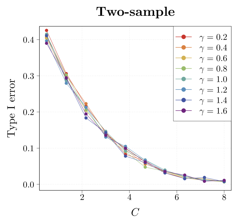
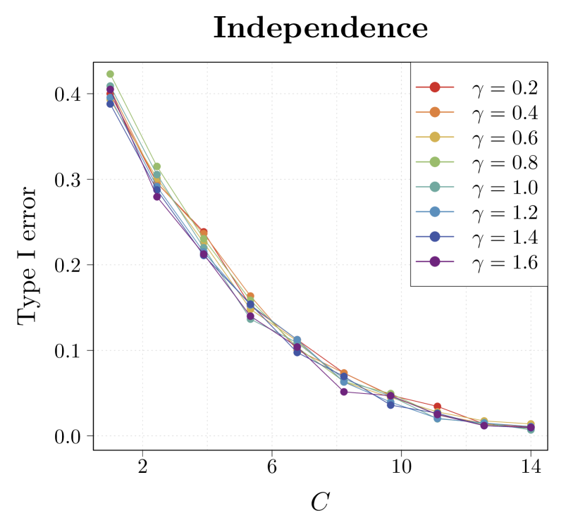
Figure 3: Type I error rates of the tests based on concentration bounds by varying constant $C$ in their thresholds. Here we approximated the type I error rates via Monte-Carlo simulations under different power law distributions with parameter $\gamma$. The results show that the error rates vary considerably depending on the choice of $C$.

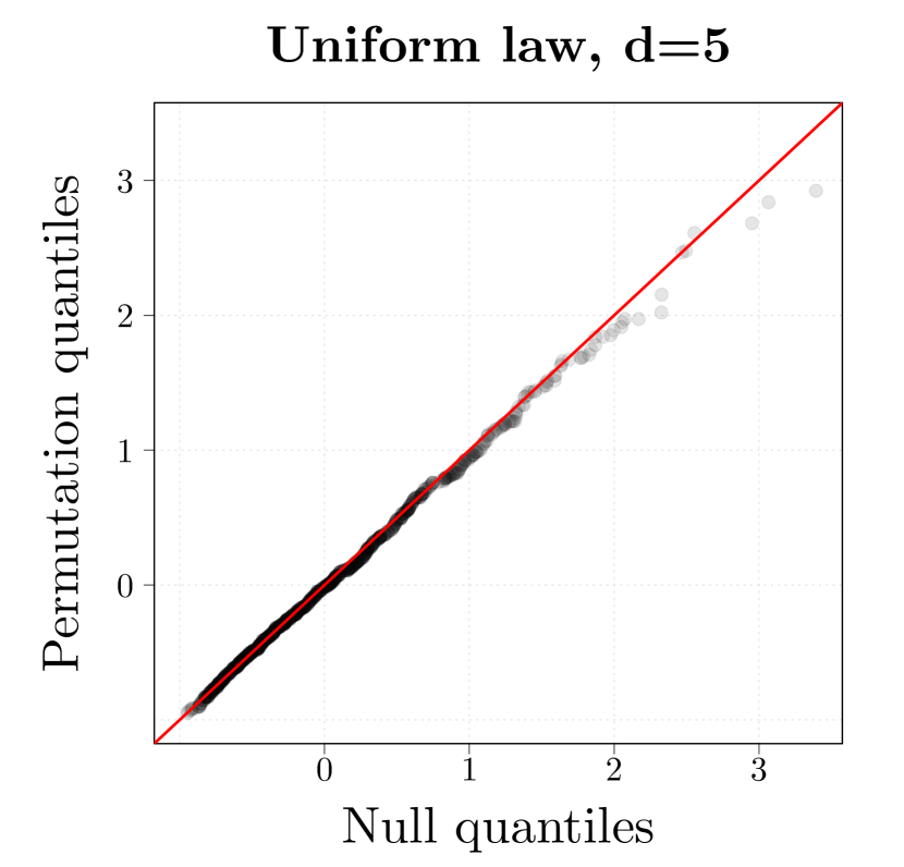
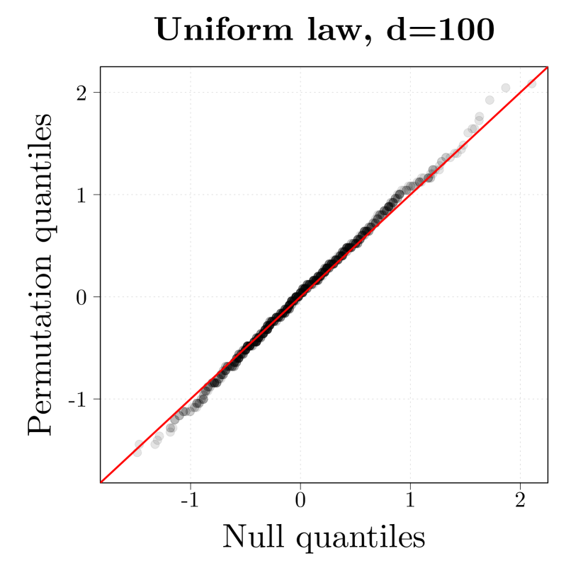
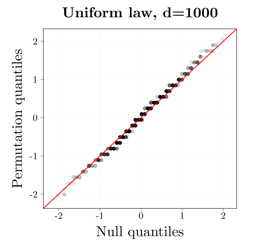
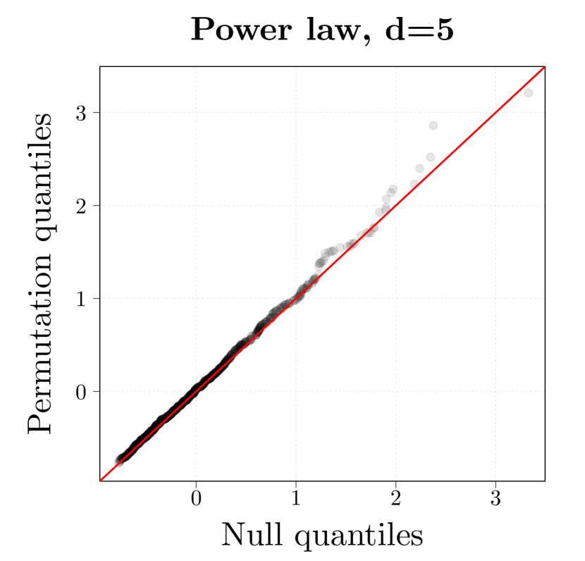
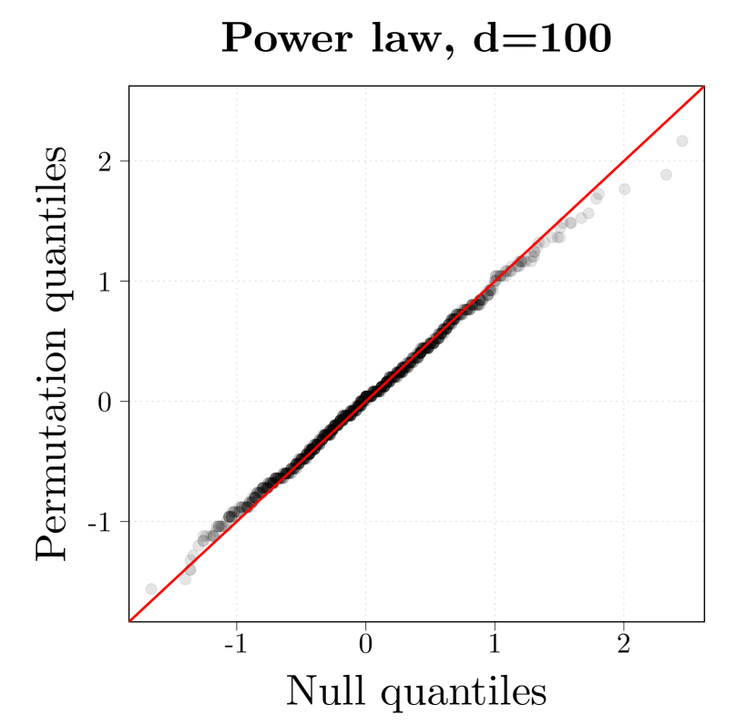
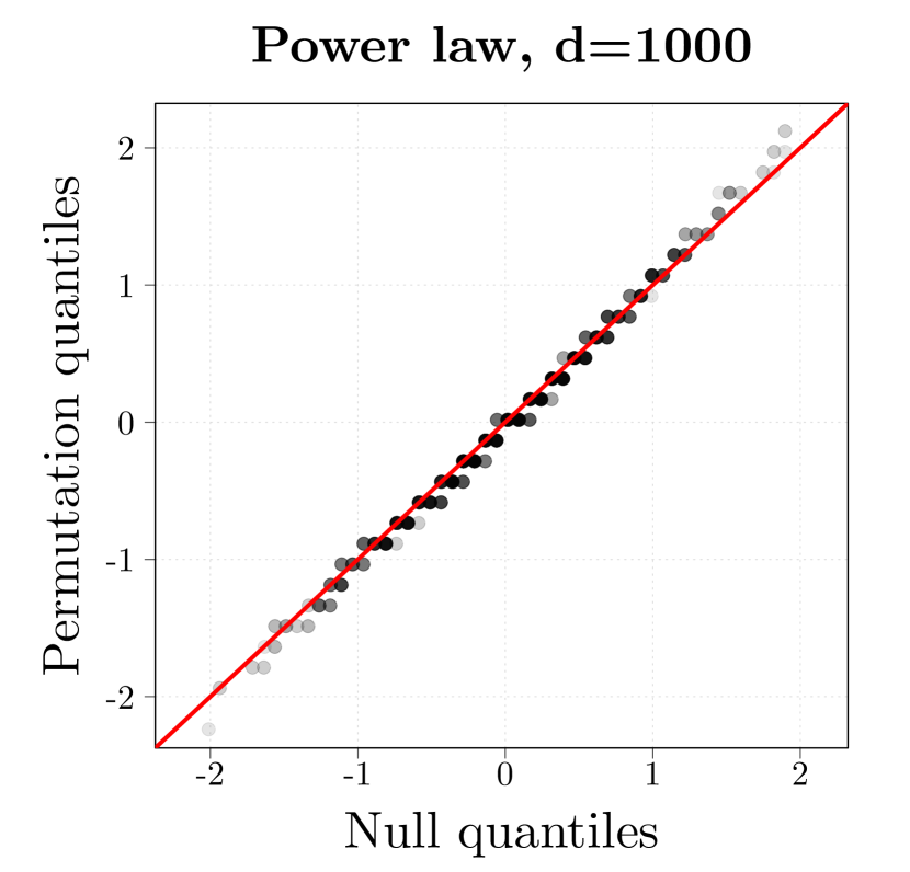
Figure 4: Q-Q plots between the null distribution and the permutation distribution of the two-sample $U$-statistic. The quantiles of the two distributions approximately lie on the straight line $y=x$ in all cases, which demonstrates the similarity of the two distributions. Here we rescaled the test statistic by an appropriate constant for display purpose only.

It has been demonstrated by several authors (e.g. Hoeffding,, 1952) that the permutation distribution of a test statistic mimics the underlying null distribution of the same test statistic in low-dimensional settings. In the next simulation, we provide empirical evidence that the same conclusion still holds in high-dimensional settings. This may further imply that the power of the permutation test approximates that of the theoretical test based on the null distribution of the test statistic. To illustrate, we focus on the two-sample $U$-statistic for multinomial testing in Proposition 4.3 and consider two different scenarios as follows.

1. Uniform law under the null. We simulate $n_{1}=n_{2}=200$ samples from the uniform multinomial distributions under the null such that $p_{Y}(k)=p_{Z}(k)=1/d$ for $k=1,\ldots,d$ where $d\in\{5,100,1000\}$. Conditional on these samples, we compute the permutation distribution of the test statistic. On the other hand, the null distribution of the test statistic is estimated based on $n_{1}=n_{2}=200$ samples from the uniform distribution by running a Monte-Carlo simulation with 2000 repetitions.

2. Power law under the alternative. In order to argue that the power of the permutation test is similar to that of the theoretical test, we need to study the behavior of the permutation distribution under the alternative. For this reason, we simulate $n_{1}=200$ samples from the uniform distribution $p_{Y}(k)=1/d$ and $n_{2}=200$ samples from the power law distribution $p_{Z}(k)\propto k$ for $k=1,\ldots,d$ where $d\in\{5,100,1000\}$. Conditional on these samples, we compute the permutation distribution of the test statistic. On the other hand, the null distribution of the test statistic is estimated based on $n_{1}=n_{2}=200$ samples from the mixture distribution $1/2\times p_{Y}+1/2\times p_{Z}$ with $2000$ repetitions.

In the simulation study, due to the computational difficulty of considering all possible permutations, we approximated the original permutation distribution using the Monte-Carlo method. Nevertheless the difference between the original permutation distribution and its Monte-Carlo counterpart can be made arbitrary small uniformly over the entire real line, which can be shown by using Dvoretzky-Kiefer-Wolfowitz inequality (Dvoretzky et al.,, 1956). In our simulations, we randomly sampled $2000$ permutations from the entire permutations, based on which we computed the empirical distribution of the permuted test statistic.

We recall from Figure 1 that the null distribution of the test statistic changes a lot depending on the size of $d$. In particular, it tends to be skewed to the right (similar to a $\chi^{2}$ distribution) when $d$ is small and tends to be symmetric (similar to a normal distribution) when $d$ is large. Also note that the null distribution tends to be more discrete when $d$ is large relative to the sample size. In Figure 4, we present the Q-Q plots of the null and (approximate) permutation distributions. It is apparent from the figure that the quantiles of these two distributions approximately lie along the straight line $y=x$ in all the scenarios. In other words, the permutation distribution closely follows the null distribution, regardless of the size of $d$, from which we conjecture that the null distribution and the permutation distribution might have the same even in high-dimensional settings.

10 Discussion

In this work we presented a general framework for analyzing the type II error rate of the permutation test based on the first two moments of the test statistic. We illustrated the utility of the proposed framework in the context of two-sample testing and independence testing in both discrete and continuous cases. In particular, we introduced the permutation tests based on degenerate $U$-statistics and explored their minimax optimality for multinomial testing as well as density testing. To improve a polynomial dependency on the nominal level $\alpha$, we developed exponential concentration inequalities for permuted $U$-statistics based on an idea that links permutations to i.i.d. Bernoulli random variables. The utility of the exponential bounds was highlighted by introducing adaptive tests to unknown parameters and also providing a concentration bound for Rademacher chaos under sampling without replacement.

Our work motivates several lines of future directions. First, while this paper considered the problem of unconditional independence testing, it would be interesting to extend our results to the problem of conditional independence testing. When the conditional variable is discrete, one can apply unconditional independence tests within categories and combine them, in a suitable way, to test for conditional independence. When the conditional variable is continuous, however, this strategy does not work and this has led several authors to use “local permutation” heuristics (see for instance Doran et al.,, 2014; Fukumizu et al.,, 2008; Neykov et al.,, 2021). In contrast to the two-sample and independence testing problems we have considered in our paper, even justifying the type I error control of these methods is not straightforward. Second, based on the coupling idea in Section 6, further work can be done to develop combinatorial concentration inequalities for other statistics. It would also be interesting to see whether one can obtain tighter concentration bounds, especially for $U_{n}^{\pi}$ in (32). Finally, identifying settings in which we can improve the dependence on the type II error rate $\beta$ for the two-moment method is another interesting direction for future research.

11 Acknowledgments

The authors are grateful to Arthur Gretton for pointing us to the work of Albert et al., (2022) and for helpful discussions. We would like thank Antonin Schrab for pointing out several typos in the original version of this manuscript. We thank Richard J. Samworth, Thomas Berrett, Tracy Ke, Bodhisattva Sen for their helpful comments. Finally, we thank three anonymous reviewers and an associate editor for their constructive comments. This work was partially supported by the NSF grant DMS-17130003.

Appendix A Overview of Appendix

In this supplementary material, we provide some additional results and the technical proofs omitted in the main text. The remainder of this material is organized as follows.

• In Appendix B, we develop exponential inequalities for permuted linear statistics, building on the concept of negative association.

• In Appendix C, we provide the result that improves Theorem 4.1 based on the exponential bound in Theorem 6.1 with an extra assumption that $n_{1}\asymp n_{2}$.

• In Appendix D, we show that Monte Carlo-based permutation tests can achieve the same error guarantee as the corresponding full permutation tests.

• The proof of Lemma 3.1 on the two moments method is provided in Appendix E.

• The proofs of the results on two-sample testing in Section 4 are presented in Appendix F, G, H and I.

• The proofs of the results on independence testing in Section 5 are presented in Appendix J, K, L, M and N.

• The proofs of the results on combinatorial concentration inequalities in Section 6 are presented in Appendix P and Q.

• The proofs of the results on adaptive tests in Section 7 are presented in Appendix R and S.

• The proofs of the results on multinomial tests and Gaussian kernel tests in Section 8 are presented in Appendix T, U, V and W.

• Lastly, the proof of the results in Appendix D can be found in Appendix X.

Appendix B Exponential inequalities for permuted linear statistics

Suppose that $\mathcal{X}_{n}=\{(Y_{1},Z_{1}),\ldots,(Y_{n},Z_{n})\}$ is a set of bivariate random variables where $Y_{i}\in\mathbb{R}$ and $Z_{i}\in\mathbb{R}$. Following the convention, let us write the sample means of $Y$ and $Z$ by $\overline{Y}:=n^{-1}\sum_{i=1}^{n}Y_{i}$ and $\overline{Z}:=n^{-1}\sum_{i=1}^{n}Z_{i}$, respectively. The sample covariance, which measures a linear relationship between $Y$ and $Z$, is given by

$$L_{n}:=\frac{1}{n}\sum_{i=1}^{n}(Y_{i}-\overline{Y})(Z_{i}-\overline{Z}).$$

We also call $L_{n}$ as a linear statistic as opposed to quadratic statistics or degenerate $U$-statistics considered in the main text. Let us denote the permuted linear statistic, associated with a permutation $\pi$ of $\{1,\ldots,n\}$, by

$$L_{n}^{\pi}=\frac{1}{n}\sum_{i=1}^{n}(Y_{i}-\overline{Y})(Z_{\pi_{i}}-\overline{Z}).$$

In this section, we provide two exponential concentration bounds for $L_{n}^{\pi}$ conditional on $\mathcal{X}_{n}$; namely Hoeffding-type inequality (Proposition B.2) and Bernstein-type inequality (Proposition B.3). These results have potential applications in studying the power of the permutation test based on $L_{n}$ and also concentration inequalities for sampling without replacement. We describe the second application in more detail in Appendix B.1 after we develop the results.

Related work and negative association. We should note that the same problem has been considered by several authors using Stein’s method (Chatterjee,, 2007), a martingale method (Chapter 4.2 of Bercu et al.,, 2015) and Talagrand’s inequality (Albert,, 2019). In fact they consider a more general linear statistic which has the form of $\sum_{i=1}^{n}d_{i,\pi_{i}}$ where $\{d_{i,j}\}_{i,j=1}^{n}$ is an arbitrary bivariate sequence. Thus their statistic includes $L_{n}$ as a special case by letting $d_{i,\pi_{i}}=(Y_{i}-\overline{Y})(Z_{\pi_{i}}-\overline{Z})$. However their proofs are quite involved at the expense of being more general. Here we provide a much simpler proof with sharper constant factors by taking advantage of the decomposability of $d_{i,j}$. To this end, we utilize the concept of negative association (e.g. Joag-Dev and Proschan,, 1983; Dubhashi and Ranjan,, 1998), defined as follows.

Definition B.1 (Negative association).

Random variables $X_{1},\ldots,X_{n}$ are negatively associated (NA) if for every two disjoint index sets $\mathcal{I},\mathcal{J}\subseteq\{1,\ldots,n\}$,

$$\mathbb{E}[f(X_{i},i\in\mathcal{I})g(X_{j},j\in\mathcal{J})]\leq\mathbb{E}[f(X_{i},i\in\mathcal{I})]\mathbb{E}[g(X_{j},j\in\mathcal{J})]$$

for all functions $f:\mathbb{R}^{|\mathcal{I}|}\mapsto\mathbb{R}$ and $g:\mathbb{R}^{|\mathcal{J}|}\mapsto\mathbb{R}$ that are both non-decreasing or both non-increasing.

Let us state several useful facts about negatively associated random variables that we shall leverage to prove the main results of this section. The proofs of the given facts can be found in Joag-Dev and Proschan, (1983) and Dubhashi and Ranjan, (1998).

• Fact 1. Let $\{x_{1},\ldots,x_{n}\}$ be a set of $n$ real values. Suppose that $\{X_{1},\ldots,X_{n}\}$ are random variables with the probability such that

  $$\mathbb{P}(X_{1}=x_{\pi_{1}},\ldots,X_{n}=x_{\pi_{n}})=\frac{1}{n!}\quad\text{for any permutation $\pi$ of $\{1,\ldots,n\}$.}$$

  Then $\{X_{1},\ldots,X_{n}\}$ are negatively associated.

• Fact 2. Let $\{X_{1},\ldots,X_{n}\}$ be negatively associated. Let $\mathcal{I}_{1},\ldots,\mathcal{I}_{k}\subseteq\{1,\ldots,n\}$ be disjoint index sets, for some positive integer $k$. For $j\in\{1,\ldots,n\}$, let $h_{j}:\mathbb{R}^{|\mathcal{I}_{k}|}\mapsto\mathbb{R}$ be functions that are all non-decreasing or all non-increasing and define $Y_{j}=h_{j}(X_{i},i\in\mathcal{I}_{j})$. Then $\{Y_{1},\ldots,Y_{k}\}$ are also negatively associated.

• Fact 3. Let $\{X_{1},\ldots,X_{n}\}$ be negatively associated. Then for any non-decreasing functions $f_{i}$, $i\in\{1,\ldots,n\}$, we have that

  $$\mathbb{E}\bigg{[}\prod_{i=1}^{n}f_{i}(X_{i})\bigg{]}\leq\prod_{i=1}^{n}\mathbb{E}[f_{i}(X_{i})].$$ (51)

Description of the main idea. Notice that $L_{n}^{\pi}$ is a function of non-i.i.d. random variables for which standard techniques relying on i.i.d. assumptions do not work directly. We avoid this difficulty by connecting $L_{n}^{\pi}$ with negatively associated random variables and then applying Chernoff bound combined with the inequality (51). The details are as follows. For notational simplicity, let us denote

$$\{a_{1},\ldots,a_{n}\}=\{Y_{1}-\overline{Y},\ldots,Y_{n}-\overline{Y}\}\quad\text{and}$$

$$\{b_{\pi_{1}},\ldots,b_{\pi_{n}}\}=\{Z_{\pi_{1}}-\overline{Z},\ldots,Z_{\pi_{n}}-\overline{Z}\}.$$

To proceed, we make several important observations.

• Observation 1. First, since $\{b_{\pi_{1}},\ldots,b_{\pi_{n}}\}$ has a permutation distribution, we can use Fact 1 and conclude that $\{b_{\pi_{1}},\ldots,b_{\pi_{n}}\}$ are negatively associated.

• Observation 2. Second, let $\mathcal{I}_{+}$ be the set of indices such that $a_{i}>0$ and similarly $\mathcal{I}_{-}$ be the set of indices such that $a_{i}<0$. Since $h_{i}(X_{i},i\in\mathcal{I}_{+})=a_{i}X_{i}$ is non-decreasing function and $h_{i}(X_{i},i\in\mathcal{I}_{-})=a_{i}X_{i}$ is non-increasing functions, it can be seen that $\{a_{i}b_{\pi_{i}}\}_{i\in\mathcal{I}_{+}}$ and $\{a_{i}b_{\pi_{i}}\}_{i\in\mathcal{I}_{-}}$ are negatively associated by Fact 2. Using this notation, the linear statistic can be written as

  $$L_{n}^{\pi}=\frac{1}{n}\sum_{i\in\mathcal{I}_{+}}a_{i}b_{\pi_{i}}+\frac{1}{n}\sum_{i\in\mathcal{I}_{-}}a_{i}b_{\pi_{i}}.$$

  It can be easily seen that $\mathbb{E}_{\pi}[b_{\pi_{i}}|\mathcal{X}_{n}]=0$ for each $i$ and thus $\mathbb{E}_{\pi}[L_{n}^{\pi}|\mathcal{X}_{n}]=0$ by linearity of expectation. Hence, for $\lambda>0$, applying the Chernoff bound yields

  $$\mathbb{P}_{\pi}(L_{n}^{\pi}\geq t|\mathcal{X}_{n})$$

  $$\leq~{} e^{-\lambda t}\mathbb{E}_{\pi}\Bigg{[}\exp\Bigg{(}\lambda n^{-1}\sum_{i\in\mathcal{I}_{+}}a_{i}b_{\pi_{i}}+\lambda n^{-1}\sum_{i\in\mathcal{I}_{-}}a_{i}b_{\pi_{i}}\Bigg{)}\Bigg{|}\mathcal{X}_{n}\Bigg{]}$$

  $$\leq~{} \frac{e^{-\lambda t}}{2}\mathbb{E}_{\pi}\Bigg{[}\exp\Bigg{(}2\lambda n^{-1}\sum_{i\in\mathcal{I}_{+}}a_{i}b_{\pi_{i}}\Bigg{)}\Bigg{|}\mathcal{X}_{n}\Bigg{]}+\frac{e^{-\lambda t}}{2}\mathbb{E}_{\pi}\Bigg{[}\exp\Bigg{(}2\lambda n^{-1}\sum_{i\in\mathcal{I}_{-}}a_{i}b_{\pi_{i}}\Bigg{)}\Bigg{|}\mathcal{X}_{n}\Bigg{]}$$

  $$:=~{} (I)+(II),$$

  where the last inequality uses the elementary inequality $xy\leq x^{2}/2+y^{2}/2$.

• Observation 3. Third, based on fact that $\{a_{i}b_{\pi_{i}}\}_{i\in\mathcal{I}_{+}}$ and $\{a_{i}b_{\pi_{i}}\}_{i\in\mathcal{I}_{-}}$ are negatively associated, we may apply Fact 3 to have that

  $$(I)~{}\leq~{}\frac{e^{-\lambda t}}{2}\prod_{i\in\mathcal{I}_{+}}\mathbb{E}_{\widetilde{b}}\big{[}\exp\big{(}2\lambda n^{-1}a_{i}\widetilde{b}_{i}\big{)}\big{|}\mathcal{X}_{n}\big{]}=\frac{e^{-\lambda t}}{2}\prod_{i=1}^{n}\mathbb{E}_{\widetilde{b}}\big{[}\exp\big{(}2\lambda n^{-1}a_{i}^{+}\widetilde{b}_{i}\big{)}\big{|}\mathcal{X}_{n}\big{]}\quad\text{and}$$ (52)

  $$(II)~{}\leq~{}\frac{e^{-\lambda t}}{2}\prod_{i\in\mathcal{I}_{-}}\mathbb{E}_{\widetilde{b}}\big{[}\exp\big{(}2\lambda n^{-1}a_{i}\widetilde{b}_{i}\big{)}\big{|}\mathcal{X}_{n}\big{]}=\frac{e^{-\lambda t}}{2}\prod_{i=1}^{n}\mathbb{E}_{\widetilde{b}}\big{[}\exp\big{(}-2\lambda n^{-1}a_{i}^{-}\widetilde{b}_{i}\big{)}\big{|}\mathcal{X}_{n}\big{]},$$

  where $\widetilde{b}_{1},\ldots,\widetilde{b}_{n}$ are i.i.d. random variables uniformly distributed over $\{b_{1},\ldots,b_{n}\}$. Here $a_{i}^{+}$ and $a_{i}^{-}$ represent $a_{i}^{+}=a_{i}\mathds{1}(a_{i}\geq 0)$ and $a_{i}^{-}=-a_{i}\mathds{1}(a_{i}\leq 0)$ respectively.

With these upper bounds for $(I)$ and $(II)$ in place, we are now ready to present the main results of this section. The first one is a Hoeffding-type bound which provides a sharper constant factor than Duembgen, (1998).

Proposition B.2 (Hoeffding-type bound).

Let us define $a_{\text{\emph{range}}}:=Y_{n}-Y_{1}$ and $b_{\text{\emph{range}}}:=Z_{n}-Z_{1}$. Then

$$\mathbb{P}_{\pi}(L_{n}^{\pi}\geq t|\mathcal{X}_{n})\leq\exp\Bigg{[}-\max\Bigg{\{}\frac{n^{2}t^{2}}{a_{\text{\emph{range}}}^{2}\sum_{i=1}^{n}b_{i}^{2}},~{}\frac{n^{2}t^{2}}{b_{\text{\emph{range}}}^{2}\sum_{i=1}^{n}a_{i}^{2}}\Bigg{\}}\Bigg{]}.$$

Proof.

The proof directly follows by applying Hoeffding’s lemma (Hoeffding,, 1963), which states that when $Z$ has zero mean and $a\leq Z\leq b$,

$$\mathbb{E}[e^{\lambda Z}]\leq e^{\lambda^{2}(b-a)^{2}/8}.$$

Notice that Hoeffding’s lemma yields

$$\prod_{i=1}^{n}\mathbb{E}_{\widetilde{b}}\big{[}\exp\big{(}2\lambda n^{-1}a_{i}^{+}\widetilde{b}_{i}\big{)}\big{|}\mathcal{X}_{n}\big{]}\leq\exp\Bigg{\{}\frac{\lambda^{2}b_{\text{range}}^{2}}{2n^{2}}\sum_{i=1}^{n}(a_{i}^{+})^{2}\Bigg{\}}\leq\exp\Bigg{\{}\frac{\lambda^{2}b_{\text{range}}^{2}}{2n^{2}}\sum_{i=1}^{n}a_{i}^{2}\Bigg{\}}\quad\text{and}$$

$$\prod_{i=1}^{n}\mathbb{E}_{\widetilde{b}}\big{[}\exp\big{(}2\lambda n^{-1}a_{i}^{-}\widetilde{b}_{i}\big{)}\big{|}\mathcal{X}_{n}\big{]}\leq\exp\Bigg{\{}\frac{\lambda^{2}b_{\text{range}}^{2}}{2n^{2}}\sum_{i=1}^{n}(a_{i}^{-})^{2}\Bigg{\}}\leq\exp\Bigg{\{}\frac{\lambda^{2}b_{\text{range}}^{2}}{2n^{2}}\sum_{i=1}^{n}a_{i}^{2}\Bigg{\}}.$$

Thus combining the above with the upper bounds for $(I)$ and $(II)$ in (LABEL:Eq:_upper_bounds_for_I_and_II) yields

$$\mathbb{P}_{\pi}(L_{n}^{\pi}\geq t|\mathcal{X}_{n})\leq\exp\Bigg{\{}-\lambda t+\frac{\lambda^{2}b_{\text{range}}^{2}}{2n^{2}}\sum_{i=1}^{n}a_{i}^{2}\Bigg{\}}.$$

By optimizing over $\lambda$ on the right-hand side, we obtain that

$$\mathbb{P}_{\pi}(L_{n}^{\pi}\geq t|\mathcal{X}_{n})\leq\exp\Bigg{\{}-\frac{n^{2}t^{2}}{b_{\text{range}}^{2}\sum_{i=1}^{n}a_{i}^{2}}\Bigg{\}}.$$ (53)

Since $\sum_{i=1}^{n}a_{\pi_{i}}b_{i}$ and $\sum_{i=1}^{n}a_{i}b_{\pi_{i}}$ have the same permutation distribution, it also holds that

$$\mathbb{P}_{\pi}(L_{n}^{\pi}\geq t|\mathcal{X}_{n})\leq\exp\Bigg{\{}-\frac{n^{2}t^{2}}{a_{\text{range}}^{2}\sum_{i=1}^{n}b_{i}^{2}}\Bigg{\}}.$$ (54)

Then putting together these two bounds (53) and (54) gives the desired result. ∎

Note that Proposition B.2 depends on the variance of either $\{a_{i}\}_{i=1}^{n}$ or $\{b_{i}\}_{i=1}^{n}$. In the next proposition, we provide a Bernstein-type bound which depends on the variance of the bivariate sequence $\{a_{i}b_{j}\}_{i,j=1}^{n}$. Similar results can be found in Bercu et al., (2015) and Albert, (2019) but in terms of constants, the bound below is much shaper than the previous ones.

Proposition B.3 (Bernstein-type bound).

Based on the same notation in Proposition B.2, a Bernstein-type bound is provided by

$$\mathbb{P}_{\pi}(L_{n}^{\pi}\geq t|\mathcal{X}_{n})\leq\exp\Bigg{\{}-\frac{nt^{2}}{2n^{-2}\sum_{i,j=1}^{n}a_{i}^{2}b_{j}^{2}+\frac{2}{3}t\max_{1\leq i,j\leq n}|a_{i}b_{j}|}\Bigg{\}}.$$

Proof.

Once we have the upper bounds for $(I)$ and $(II)$ in (LABEL:Eq:_upper_bounds_for_I_and_II), the remainder of the proof is routine. First it is straightforward to verify that for $|Z|\leq c$, $\mathbb{E}[Z]=0$ and $\mathbb{E}[Z^{2}]=\sigma^{2}$, we have that

$$\mathbb{E}[e^{\lambda Z}]=1+\sum_{k=2}^{\infty}\frac{\mathbb{E}[(\lambda Z)^{k}]}{k!}\leq 1+\frac{\sigma^{2}}{c^{2}}\sum_{k=2}^{\infty}\frac{\lambda^{k}c^{k}}{k!}\leq\exp\bigg{\{}\frac{\sigma^{2}}{c^{2}}\left(e^{\lambda c}-1-\lambda c\right)\bigg{\}}.$$

Let us write $\widehat{\sigma}_{i}^{2}=n^{-3}a_{i}^{2}\sum_{j=1}^{n}b_{i}^{2}$ and $M=n^{-1}\max_{1\leq i,j\leq n}|a_{i}b_{j}|$. Then based on the above inequality, we can obtain that

$$\prod_{i=1}^{n}\mathbb{E}_{\widetilde{b}}\big{[}\exp\big{(}2\lambda n^{-1}a_{i}^{+}\widetilde{b}_{i}\big{)}\big{|}\mathcal{X}_{n}\big{]}\leq\exp\Bigg{\{}\frac{\sum_{i=1}^{n}\widehat{\sigma}_{i}^{2}}{M^{2}}\left(e^{\lambda M}-1-\lambda M\right)\Bigg{\}}\quad\text{and}$$

$$\prod_{i=1}^{n}\mathbb{E}_{\widetilde{b}}\big{[}\exp\big{(}2\lambda n^{-1}a_{i}^{-}\widetilde{b}_{i}\big{)}\big{|}\mathcal{X}_{n}\big{]}\leq\exp\Bigg{\{}\frac{\sum_{i=1}^{n}\widehat{\sigma}_{i}^{2}}{M^{2}}\left(e^{\lambda M}-1-\lambda M\right)\Bigg{\}}.$$

Combining these two upper bounds with the result in (LABEL:Eq:_upper_bounds_for_I_and_II) yields

$$\mathbb{P}_{\pi}\left(L_{n}^{\pi}\geq t|\mathcal{X}_{n}\right)\leq e^{-\lambda t}\exp\Bigg{\{}\frac{\sum_{i=1}^{n}\widehat{\sigma}_{i}^{2}}{M^{2}}\left(e^{\lambda M}-1-\lambda M\right)\Bigg{\}}.$$

By optimizing the right-hand side in terms of $\lambda$, we obtain a Bennett-type inequality

$$\mathbb{P}_{\pi}\left(L_{n}^{\pi}\geq t|\mathcal{X}_{n}\right)\leq\exp\Bigg{\{}-\frac{\sum_{i=1}^{n}\widehat{\sigma}_{i}^{2}}{M^{2}}h\left(\frac{tM}{\sum_{i=1}^{n}\widehat{\sigma}_{i}^{2}}\right)\Bigg{\}},$$

where $h(x)=(1+x)\log(1+x)-x$. Then the result follows by noting that $h(x)\geq x^{2}/(2+2x/3)$. ∎

In the next subsection, we apply our results to derive concentration inequalities for sampling without replacement.

B.1 Concentration inequalities for sampling without replacement

To establish the explicit connection to sampling without replacement, we focus on the case where $Z_{i}$ is binary, say $Z_{i}\in\{-a,a\}$. Then the linear statistic $L_{n}$ is related to the unscaled two-sample $t$-statistic. More specifically, let us write $n_{1}=\sum_{i=1}^{n}\mathds{1}(Z_{i}=a)$ and $n_{2}=\sum_{i=1}^{n}\mathds{1}(Z_{i}=-a)$. Additionally we use the notation $\overline{Y}_{1}=n_{1}^{-1}\sum_{i=1}^{n}Y_{i}\mathds{1}(Z_{i}=a)$ and $\overline{Y}_{2}=n_{2}^{-1}\sum_{i=1}^{n}Y_{i}\mathds{1}(Z_{i}=-a)$. Then some algebra shows that the sample covariance $L_{n}$ is exactly the form of

$$L_{n}=2a\frac{n_{1}n_{2}}{n^{2}}(\overline{Y}_{1}-\overline{Y}_{2}).$$

Without loss of generality, we assume $a=1$, i.e. $Z_{i}\in\{-1,1\}$. Then Proposition B.2 gives a concentration inequality for the unscaled $t$-statistic as

$$\mathbb{P}_{\pi}\Bigg{\{}\frac{2n_{1}n_{2}}{n^{2}}\left(\overline{Y}_{1,\pi}-\overline{Y}_{2,\pi}\right)\geq t\Bigg{|}\mathcal{X}_{n}\Bigg{\}}~{}=~{} \mathbb{P}_{\pi}\Bigg{\{}\left(\overline{Y}_{1,\pi}-\overline{Y}_{2,\pi}\right)\geq\frac{tn^{2}}{2n_{1}n_{2}}\Bigg{|}\mathcal{X}_{n}\Bigg{\}}$$

$$\leq~{} \exp\Bigg{\{}-\frac{n^{2}t^{2}}{4\sum_{i=1}^{n}(Y_{i}-\overline{Y})^{2}}\Bigg{\}},$$

where $\overline{Y}_{1,\pi}=n_{1}^{-1}\sum_{i=1}^{n}Y_{\pi_{i}}\mathds{1}(Z_{i}=1)$ and $\overline{Y}_{2,\pi}=n_{2}^{-1}\sum_{i=1}^{n}Y_{\pi_{i}}\mathds{1}(Z_{i}=-1)$. This implies that

$$\mathbb{P}_{\pi}\left(\overline{Y}_{1,\pi}-\overline{Y}_{2,\pi}\geq t\big{|}\mathcal{X}_{n}\right)\leq\exp\left(-\frac{n_{1}^{2}n_{2}^{2}t^{2}}{n^{3}\widehat{\sigma}_{\text{lin}}^{2}}\right),$$

where $\widehat{\sigma}_{\text{lin}}^{2}=n^{-1}\sum_{i=1}^{n}(Z_{i}-\overline{Z})^{2}$. By symmetry, it also holds that

$$\mathbb{P}_{\pi}\left(|\overline{Y}_{1,\pi}-\overline{Y}_{2,\pi}|\geq t\big{|}\mathcal{X}_{n}\right)\leq 2\exp\left(-\frac{n_{1}^{2}n_{2}^{2}t^{2}}{n^{3}\widehat{\sigma}_{\text{lin}}^{2}}\right).$$

Let us denote the sample mean of the entire samples by $\overline{Y}=n^{-1}\sum_{i=1}^{n}Y_{i}$. Then using the exact relationship

$$|\overline{Y}_{1,\pi}-\overline{Y}_{2,\pi}|=\frac{n}{n_{2}}|\overline{Y}_{1,\pi}-\overline{Y}|,$$ (55)

the above inequality is equivalent to

$$\mathbb{P}_{\pi}\left(|\overline{Y}_{1,\pi}-\overline{Y}|\geq t\big{|}\mathcal{X}_{n}\right)\leq 2\exp\left(-\frac{n_{1}^{2}t^{2}}{n\widehat{\sigma}_{\text{lin}}^{2}}\right).$$ (56)

Notice that $\overline{Y}_{1,\pi}$ is the sample mean of $n_{1}$ observations sampled without replacement from $\{Y_{1},\ldots,Y_{n}\}$. This implies that the permutation law of the sample mean is equivalent to the probability law under sampling without replacement. The same result (including the constant factor) exists in Massart, (1986) (see Lemma 3.1 therein). However, the result given there only holds when $n=n_{1}\times m$ where $m$ is a positive integer whereas our result does not require such restriction.

An improvement via Berstein-type bound. Although the tail bound (56) is simple depending only on the variance term $\widehat{\sigma}_{\text{lin}}^{2}$, it may not be effective when $n_{1}$ is much smaller than $n$ (e.g. $n_{1}^{2}/n\rightarrow 0$ as $n_{1}\rightarrow\infty$). In such case, Proposition B.3 gives a tighter bound. More specifically, following the same steps as before, Proposition B.3 presents a concentration inequality for the two-sample (unscaled) $t$-statistic as

$$\mathbb{P}_{\pi}(L_{n}^{\pi}\geq t|\mathcal{X}_{n})~{}=~{} \mathbb{P}_{\pi}\Bigg{\{}\left(\overline{Y}_{1,\pi}-\overline{Y}_{2,\pi}\right)\geq\frac{tn^{2}}{2n_{1}n_{2}}\Bigg{|}\mathcal{X}_{n}\Bigg{\}}$$

$$~{}\leq~{} \exp\Bigg{\{}-\frac{nt^{2}}{8\frac{n_{1}n_{2}}{n^{2}}\widehat{\sigma}_{\text{lin}}^{2}+\frac{4}{3}t\cdot\max\left(\frac{n_{1}}{n},\frac{n_{2}}{n}\right)\cdot M_{Z}}\Bigg{\}},$$

where $M_{Z}:=\max_{1\leq i\leq n}|Z_{i}-\overline{Z}|$. Furthermore, using the relationship (55) and by symmetry,

$$\mathbb{P}_{\pi}\left(|\overline{Y}_{1,\pi}-\overline{Y}|\geq t\big{|}\mathcal{X}_{n}\right)\leq 2\exp\Bigg{\{}-\frac{12n_{1}t^{2}}{24\frac{n_{2}}{n}\widehat{\sigma}_{\text{lin}}^{2}+8\frac{n_{2}}{n}M_{Z}t}\Bigg{\}},$$ (57)

where we assumed $n_{1}\leq n_{2}$.

Remark B.4.

We remark that the bounds in (56) and (57) are byproducts of more general bounds and are not necessary the sharpest ones in the context of sampling without replacement. We refer to Bardenet and Maillard, (2015) and among others for some recent developments of concentration bounds for sampling without replacement.

Appendix C Improved version of Theorem 4.1

In this section, we improve the result of Theorem 4.1 based on the exponential bound in Theorem 6.1. In particular we replace the dependency on $\alpha^{-1}$ there with $\log(1/\alpha)$ by adding an extra assumption that $n_{1}\asymp n_{2}$ as follows.

Lemma C.1 (Two-sample $U$-statistic).

For $0<\alpha<e^{-1}$, suppose that there is a sufficiently large constant $C>0$ such that

$$\mathbb{E}_{P}[U_{n_{1},n_{2}}]\geq C\max\Bigg{\{}\sqrt{\frac{\psi_{Y,1}(P)}{\beta n_{1}}},\ \sqrt{\frac{\psi_{Z,1}(P)}{\beta n_{2}}},\ \sqrt{\frac{\psi_{YZ,2}(P)}{\beta}}\log\left(\frac{1}{\alpha}\right)\cdot\left(\frac{1}{n_{1}}+\frac{1}{n_{2}}\right)\Bigg{\}},$$ (58)

for all $P\in\mathcal{P}_{1}\subset\mathcal{P}_{h_{\text{\emph{ts}}}}$. Then under the assumptions that $n_{1}\asymp n_{2}$, the type II error of the permutation test over $\mathcal{P}_{1}$ is uniformly bounded by $\beta$, that is

$$\sup_{P\in\mathcal{P}_{1}}\mathbb{P}_{P}^{(n_{1},n_{2})}(U_{n_{1},n_{2}}\leq c_{1-\alpha,n_{1},n_{2}})\leq\beta.$$

Proof.

To prove the above lemma, we employ the quantile approach described in Section 3 (see also Fromont et al.,, 2013). More specifically we let $q_{1-\beta/2,n}$ denote the quantile of the permutation critical value $c_{1-\alpha,n}$ of $U_{n_{1},n_{2}}$. Then as shown in the proof of Lemma 3.1, if

$$\mathbb{E}_{P}[U_{n_{1},n_{2}}]~{}\geq~{}q_{1-\beta/2,n}+\sqrt{\frac{2\text{Var}_{P}[U_{n_{1},n_{2}}]}{\beta}},$$

then the type II error of the permutation test is controlled as

$$\sup_{P\in\mathcal{P}_{1}}\mathbb{P}_{P}(U_{n_{1},n_{2}}\leq c_{1-\alpha,n})~{}\leq~{} \sup_{P\in\mathcal{P}_{1}}\mathbb{P}_{P}(U_{n_{1},n_{2}}\leq q_{1-\beta/2,n})+\sup_{P\in\mathcal{P}_{1}}\mathbb{P}_{P}(q_{1-\beta/2,n}<c_{1-\alpha,n})$$

$$\leq~{} \beta.$$

Therefore it is enough to verify that the right-hand side of (58) is lower bounded by $q_{1-\beta/2,n}+\sqrt{2\text{Var}_{P}[U_{n_{1},n_{2}}]/\beta}$. As shown in the proof of Theorem 4.1, the variance is bounded by

$$\text{Var}_{P}[U_{n_{1},n_{2}}]\leq C_{1}\frac{\psi_{Y,1}(P)}{n_{1}}+C_{2}\frac{\psi_{Z,1}(P)}{n_{2}}+C_{3}\psi_{YZ,2}(P)\left(\frac{1}{n_{1}}+\frac{1}{n_{2}}\right)^{2}.$$ (59)

Moving onto an upper bound for $q_{1-\beta/2,n}$, let us denote

$$\Sigma_{n_{1},n_{2}}^{\dagger}:=\frac{1}{n_{1}^{2}(n_{1}-1)^{2}}\sum_{(i_{1},i_{2})\in\mathbf{i}_{2}^{n}}g^{2}(X_{i_{1}},X_{i_{2}}).$$

From Theorem 6.1 together with the trivial bound (31), we know that $c_{1-\alpha,n}$ is bounded by

$$c_{1-\alpha,n} ~{}\leq~{}\max\Bigg{\{}\sqrt{\frac{\Sigma_{n_{1},n_{2}}^{\dagger 2}}{C_{4}}\log\left(\frac{1}{\alpha}\right)},\ \frac{\Sigma_{n_{1},n_{2}}^{\dagger}}{C_{4}}\log\left(\frac{1}{\alpha}\right)\Bigg{\}}$$ (60)

$$~{}\leq~{}C_{5}\Sigma_{n_{1},n_{2}}^{\dagger}\log\left(\frac{1}{\alpha}\right),$$

where the last inequality uses the assumption that $\alpha<e^{-1}$. Now applying Markov’s inequality yields

$$\mathbb{P}_{P}\left(\Sigma_{n_{1},n_{2}}^{\dagger}\geq t\right)\leq\frac{\mathbb{E}_{P}[\Sigma_{n_{1},n_{2}}^{\dagger 2}]}{t^{2}}\leq C_{6}\frac{\psi_{YZ,2}(P)}{t^{2}n_{1}^{2}}.$$

By setting the right-hand side to be $\beta/2$, we can find an upper bound for the $1-\beta/2$ quantile of $\Sigma_{n_{1},n_{2}}^{\dagger}$. Combining this observation with inequality (60) yields

$$q_{1-\beta/2,n}\leq\frac{C_{7}}{\beta^{1/2}}\log\left(\frac{1}{\alpha}\right)\frac{\sqrt{\psi_{YZ,2}(P)}}{n_{1}}.$$

Therefore, from the above bound and (59),

$$q_{1-\beta/2,n}+\sqrt{\frac{2\text{Var}_{P}[U_{n_{1},n_{2}}]}{\beta}}$$

$$\leq~{} C\sqrt{\max\Bigg{\{}\frac{\psi_{Y,1}(P)}{\beta n_{1}},\ \frac{\psi_{Z,1}(P)}{\beta n_{2}},\ \frac{\psi_{YZ,2}(P)}{\beta}\log^{2}\left(\frac{1}{\alpha}\right)\cdot\left(\frac{1}{n_{1}}+\frac{1}{n_{2}}\right)^{2}\Bigg{\}}}.$$

This completes the proof of Lemma C.1. ∎

Appendix D Monte Carlo-based permutation tests

As mentioned in Remark 2.1, exact calculation of a permutation test is computationally infeasible for large sample sizes. To mitigate this computational issue, it is now standard to consider a Monte Carlo-based (MC-based) permutation test in practical applications. The goal of this section is to demonstrate that this MC-based permutation test can achieve the same minimax rate optimality as the original permutation test, while controlling the type I error rate. Of course, this guarantee requires a sufficiently large number of Monte Carlo samples and we show that this number depends on the pre-specified type I and II error rates $\alpha$ and $\beta$, but not on the sample size.

To fix ideas, let $\pi_{1},\ldots,\pi_{B}$ be random permutations uniformly sampled with replacement from $\mathbf{\Pi}_{n}$, where we recall that $\mathbf{\Pi}_{n}$ is the set of all possible permutations of $\{1,\ldots,n\}$. Then the MC-based permutation $p$-value is given by

$$\widehat{p}:=\frac{1}{B+1}\bigg{\{}1+\sum_{i=1}^{B}\mathds{1}\big{(}T_{n}^{\pi_{i}}\geq T_{n}\big{)}\bigg{\}}=\frac{1}{B+1}\sum_{i=1}^{B+1}\mathds{1}\big{(}T_{n}^{\pi_{i}}\geq T_{n}\big{)},$$ (61)

where we define $T_{n}^{\pi_{B+1}}:=T_{n}$. It is worth pointing out that adding the identity permutation is required to control the type I error rate in finite sample sizes (e.g. Phipson and Smyth,, 2010). In particular, we have $\mathbb{P}(\widehat{p}\leq\alpha)\leq\alpha$ whenever $\mathcal{X}_{n}$ and $\mathcal{X}_{n}^{\pi}$ have the same distribution for every $\pi\in\mathbf{\Pi}_{n}$. A formal proof of this statement can be found, for example, in Hemerik and Goeman, (2018). Let $\widehat{c}_{1-\alpha,n}$ be the $1-\alpha$ quantile of the distribution with random permutations defined as

$$\widehat{c}_{1-\alpha,n}~{}:={} \inf\bigg{\{}t:\frac{1}{B+1}\sum_{i=1}^{B+1}\mathds{1}\big{(}T_{n}^{\pi_{i}}\leq t\big{)}\geq 1-\alpha\bigg{\}}.$$ (62)

Then it can be verified that the MC-based permutation test can be equivalently written as $\mathds{1}(\widehat{p}\leq\alpha)=\mathds{1}(T_{n}>\widehat{c}_{1-\alpha,n})$. Intuitively, when $B$ is sufficiently large, $\widehat{c}_{1-\alpha,n}$ becomes close to $c_{1-\alpha,n}$, the $1-\alpha$ quantile of the original permutation distribution. Consequently, the type II error of the MC-based permutation test should approximate that of the original permutation test $\mathds{1}(T_{n}>c_{1-\alpha,n})$. The next proposition formalizes this intuition by reproducing Lemma 3.1 for the MC-based permutation test.

Proposition D.1 (Two-moment method for MC-based tests).

Suppose that for each permutation $\pi\in\mathbf{\Pi}_{n}$, $T_{n}$ and $T_{n}^{\pi}$ have the same distribution under the null hypothesis. Given pre-specified error rates $\alpha\in(0,1)$ and $\beta\in(0,1-\alpha)$, assume that for any $P\in\mathcal{P}_{1}$,

$$\mathbb{E}_{P}[T_{n}]~{}\geq{} \mathbb{E}_{P}[\mathbb{E}_{\pi}\{T_{n}^{\pi}|\mathcal{X}_{n}\}]+\sqrt{\frac{6\emph{\text{Var}}_{P}[\mathbb{E}_{\pi}\{T_{n}^{\pi}|\mathcal{X}_{n}\}]}{\beta}}$$ (63)

$$+\sqrt{\frac{6\emph{\text{Var}}_{P}[T_{n}]}{\beta}}+\sqrt{\frac{12\mathbb{E}_{P}[\emph{\text{Var}}_{\pi}\{T_{n}^{\pi}|\mathcal{X}_{n}\}]}{\alpha\beta}}.$$

Suppose further that the number of Monte Carlo simulations $B$ is greater than $B\geq 8\alpha^{-2}\log(4/\beta)$. Then the MC-based permutation test $\mathds{1}(\widehat{p}\leq\alpha)$ controls the type I and II error rates as in (LABEL:Eq:_uniform_error_control) where $\widehat{p}$ is defined in (61).

We present several remarks on Proposition D.1.

Remark D.2.

• The new condition (63) is the same as the condition for the full permutation test in Lemma 3.1 up to constant factors. In other words, the MC-based permutation test can achieve the same error guarantee as the original permutation test by adjusting constant factors.
  

• Using Proposition D.1 and its modification, we can reproduce the rate optimality results of the permutation test based on the Monte Carlo counterpart.
  

• The proof of Proposition D.1 is based on Dvoretzky–Kiefer–Wolfowitz inequality. Using this, we verify the type II error can be bounded by

  $$\mathbb{P}_{P}^{(n)}(\widehat{p}>\alpha)~{}\leq~{}\mathbb{P}_{P}^{(n)}(T_{n}\leq c_{1-\alpha^{\ast}})+\beta/2,$$

  where $1-\alpha^{\ast}=\frac{B+1}{B}(1-\alpha)+\sqrt{\frac{1}{2B}\log\left(4/\beta\right)}$. We then build on Lemma 3.1 and show that $\mathbb{P}_{P}(T_{n}\leq c_{1-\alpha^{\ast}})\leq\beta/2$ under the given condition to complete the proof. The details can be found in Appendix X.
  

• It is interesting to point out that the condition for $B$ is independent of the sample size $n$. This may be explained by the fact that the distance between $\widehat{c}_{1-\alpha,n}$ and $c_{1-\alpha,n}$ can be made small independent of $n$.

Appendix E Proof of Lemma 3.1

As discussed in the main text, the key difficulty of studying the type II error of the permutation test lies in the fact that its critical value is data-dependent and thereby random. Our strategy to overcome this problem is to bound the random critical value by a quantile value with high probability (see also Fromont et al.,, 2013). We split the proof of Lemma 3.1 into three steps. In the first step, we present a sufficient condition under which the type II error of the test with a non-random cutoff value is small. In the second step, we provide a non-random upper bound for the permutation critical value, which holds with high probability. In the last step, we combine the results and complete the proof.

Step 1.

For a given $P\in\mathcal{P}_{1}$, let $\omega(P)$ be any constant depending on $P$ such that

$$\mathbb{E}_{P}[T_{n}]~{}\geq~{}\omega(P)+\sqrt{\frac{3\text{Var}_{P}[T_{n}]}{\beta}}.$$ (64)

Based on such $\omega(P)$, we define a test $\mathds{1}\{T_{n}>\omega(P)\}$, which controls the type II error by $\beta/3$. To see this, let us apply Chebyshev’s inequality

$$\beta/3~{}\geq~{} \mathbb{P}_{P}\big{(}\big{|}T_{n}-\mathbb{E}_{P}[T_{n}]\big{|}\geq\sqrt{3\beta^{-1}\text{Var}_{P}[T_{n}]}\big{)}$$

$$\geq~{} \mathbb{P}_{P}\big{(}-T_{n}+\mathbb{E}_{P}[T_{n}]\geq\sqrt{3\beta^{-1}\text{Var}_{P}[T_{n}]}\big{)}$$

$$\geq~{} \mathbb{P}_{P}\big{(}\omega(P)\geq T_{n}\big{)},$$

where the last inequality uses the condition of $\omega(P)$ in (64). In other words, the type II error of the test $\mathds{1}\{T_{n}>\omega(P)\}$ is less than or equal to $\beta/3$ as desired.

Step 2.

In this step, we provide an upper bound for $c_{1-\alpha,n}$, which may hold with high probability. First, applying Chebyshev’s inequality yields

$$\mathbb{P}_{\pi}\left(\big{|}T_{n}^{\pi}-\mathbb{E}_{\pi}[T_{n}^{\pi}|\mathcal{X}_{n}]\big{|}\geq\sqrt{\alpha^{-1}\text{Var}_{\pi}[T_{n}^{\pi}|\mathcal{X}_{n}]}~{}\big{|}\mathcal{X}_{n}\right)\leq\alpha.$$

Therefore, by the definition of the quantile, we see that $c_{1-\alpha,n}$ satisfies

$$c_{1-\alpha,n}~{}\leq~{}\mathbb{E}_{\pi}[T_{n}^{\pi}|\mathcal{X}_{n}]+\sqrt{\alpha^{-1}\text{Var}_{\pi}[T_{n}^{\pi}|\mathcal{X}_{n}]}.$$ (65)

Note that the two terms on the right-hand side are random variables depending on $\mathcal{X}_{n}$. In order to use the result from the first step, we want to further upper bound these two terms by some constants. To this end, let us define two good events:

$$\mathcal{A}_{1}:=\Big{\{}\mathbb{E}_{\pi}[T_{n}^{\pi}|\mathcal{X}_{n}]<\mathbb{E}_{P}[\mathbb{E}_{\pi}\{T_{n}^{\pi}|\mathcal{X}_{n}\}]+\sqrt{3\beta^{-1}\text{Var}_{P}[\mathbb{E}_{\pi}\{T_{n}^{\pi}|\mathcal{X}_{n}\}]}\Big{\}},$$

$$\mathcal{A}_{2}:=\Big{\{}\sqrt{\alpha^{-1}\text{Var}_{\pi}[T_{n}^{\pi}|\mathcal{X}_{n}]}<\sqrt{3\alpha^{-1}\beta^{-1}\mathbb{E}_{P}[\text{Var}_{\pi}\{T_{n}^{\pi}|\mathcal{X}_{n}\}]}\Big{\}}.$$

Then by applying Markov and Chebyshev’s inequalities, it is straightforward to see that

$$\mathbb{P}_{P}(\mathcal{A}_{1}^{c})\leq\beta/3\quad\text{and}\quad\mathbb{P}_{P}(\mathcal{A}_{2}^{c})\leq\beta/3.$$ (66)

Step 3.

Here, building on the first two steps, we conclude the result. We begin by upper bounding the type II error of the permutation test as

$$\mathbb{P}_{P}(T_{n}\leq c_{1-\alpha,n})~{}=~{} \mathbb{P}_{P}(T_{n}\leq c_{1-\alpha,n},\ \mathcal{A}_{1}\cup\mathcal{A}_{2})+\mathbb{P}_{P}(T_{n}\leq c_{1-\alpha,n},\ \mathcal{A}_{1}^{c}\cap\mathcal{A}_{2}^{c})$$

$$\leq~{} \mathbb{P}_{P}(T_{n}\leq\omega^{\prime}(P))+\mathbb{P}_{P}(\mathcal{A}_{1}^{c}\cap\mathcal{A}_{2}^{c}),$$

where, for simplicity, we write

$$\omega^{\prime}(P):=\mathbb{E}_{P}[\mathbb{E}_{\pi}\{T_{n}^{\pi}|\mathcal{X}_{n}\}]+\sqrt{3\beta^{-1}\text{Var}_{P}[\mathbb{E}_{\pi}\{T_{n}^{\pi}|\mathcal{X}_{n}\}]}+\sqrt{3\alpha^{-1}\beta^{-1}\mathbb{E}_{P}[\text{Var}_{\pi}\{T_{n}^{\pi}|\mathcal{X}_{n}\}]}.$$

One may check that the type II error of $\mathds{1}\{T_{n}>\omega^{\prime}(P)\}$ is controlled by $\beta/3$ as long as $\omega^{\prime}(P)+\sqrt{3\text{Var}_{P}[T_{n}]/\beta}\leq\mathbb{E}_{P}[T_{n}]$ from the inequality (64) in Step 1. However, this sufficient condition is ensured by condition (3) of Lemma 3.1. Furthermore, the probability of the intersection of the two bad events $\mathcal{A}_{1}^{c}\cap\mathcal{A}_{2}^{c}$ is also bounded by $2\beta/3$ due to the concentration results in (66). Hence, by taking the supremum over $P\in\mathcal{P}_{1}$, we may conclude that

$$\sup_{P\in\mathcal{P}_{1}}\mathbb{P}_{P}(T_{n}\leq c_{1-\alpha,n})\leq\beta.$$

This completes the proof of Lemma 3.1.

Appendix F Proof of Theorem 4.1

We proceed the proof by verifying the sufficient condition in Lemma 3.1. We first verify that the expectation of $U_{n_{1},n_{2}}^{\pi}$ is zero under the permutation law. Let us recall the permuted $U$-statistic $U_{n_{1},n_{2}}^{\pi}$ in (26). In fact, by the linearity of expectation, it suffices to prove

$$\mathbb{E}_{\pi}[h_{\text{ts}}(X_{\pi_{1}},X_{\pi_{2}};X_{\pi_{n_{1}+1}},X_{\pi_{n_{1}+2}})|\mathcal{X}_{n}]=0.$$

This is clearly the case by recalling the definition of kernel $h_{\text{ts}}$ in (5) and noting that the expectation $\mathbb{E}_{\pi}[g(X_{\pi_{i}},X_{\pi_{j}})|\mathcal{X}_{n}]$ is invariant to the choice of $(i,j)\in\mathbf{i}_{2}^{n}$, which leads to $\mathbb{E}_{\pi}[U_{n_{1},n_{2}}^{\pi}|\mathcal{X}_{n}]=0$. Therefore we only need to verify the simplified condition (4) under the given assumptions in Theorem 4.1.

The rest of the proof is divided into two parts. In each part, we prove the following conditions separately,

$$\mathbb{E}_{P}[U_{n_{1},n_{2}}]\geq 2\sqrt{\frac{2\text{Var}_{P}[U_{n_{1},n_{2}}]}{\beta}}\quad\text{and}$$ (67)

$$\mathbb{E}_{P}[U_{n_{1},n_{2}}]\geq 2\sqrt{\frac{2\mathbb{E}_{P}[\text{Var}_{\pi}\{U_{n_{1},n_{2}}^{\pi}|\mathcal{X}_{n}\}]}{\alpha\beta}}.$$ (68)

We then complete the proof of Theorem 4.1 by noting that (67) and (68) imply the simplified condition (4).

Part 1. Verification of condition (67). In this part, we verify condition (67). To do so, we state the explicit variance formula of a two-sample $U$-statistic (e.g. page 38 of Lee,, 1990). Following the notation of Lee, (1990), we let $\check{\sigma}_{i,j}^{2}$ denote the variance of a conditional expectation given as

$$\check{\sigma}_{i,j}^{2}=\text{Var}_{P}[\mathbb{E}_{P}\{\overline{h}_{\text{ts}}(y_{1},\ldots,y_{i},Y_{i+1},\ldots,Y_{2};z_{1},\ldots,z_{j},Z_{j+1},\ldots,Z_{2})\}]$$

for $0\leq i,j\leq 2$. Then the variance of $U_{n_{1},n_{2}}$ is given by

$$\text{Var}_{P}[U_{n_{1},n_{2}}]=\sum_{i=0}^{2}\sum_{j=0}^{2}\binom{2}{i}\binom{2}{j}\binom{n_{1}-2}{2-i}\binom{n_{2}-2}{2-j}\binom{n_{1}}{2}^{-1}\binom{n_{2}}{2}^{-1}\check{\sigma}_{i,j}^{2}.$$ (69)

By the law of total variance, one may see that $\check{\sigma}_{i,j}^{2}\leq\check{\sigma}_{2,2}^{2}$ for all $0\leq i,j\leq 2$. This leads to an upper bound for $\text{Var}_{P}[U_{n_{1},n_{2}}]$ as

$$\text{Var}_{P}[U_{n_{1},n_{2}}]\leq C_{1}\frac{\check{\sigma}_{1,0}^{2}}{n_{1}}+C_{2}\frac{\check{\sigma}_{0,1}^{2}}{n_{2}}+C_{3}\left(\frac{1}{n_{1}}+\frac{1}{n_{2}}\right)^{2}\check{\sigma}_{2,2}^{2}.$$

Now applying Jensen’s inequality, repeatedly, yields

$$\check{\sigma}_{2,2}^{2}\leq\mathbb{E}_{P}[\overline{h}_{\text{ts}}^{2}(Y_{1},Y_{2};Z_{1},Z_{2})]\leq\mathbb{E}_{P}[h_{\text{ts}}^{2}(Y_{1},Y_{2};Z_{1},Z_{2})]\leq C_{4}\psi_{YZ,2}(P).$$

Then by noting that $\check{\sigma}_{1,0}^{2}$ and $\check{\sigma}_{0,1}^{2}$ correspond to the notation $\psi_{Y,1}(P)$ and $\psi_{Z,1}(P)$, respectively,

$$\text{Var}_{P}[U_{n_{1},n_{2}}]\leq C_{1}\frac{\psi_{Y,1}(P)}{n_{1}}+C_{2}\frac{\psi_{Z,1}(P)}{n_{2}}+C_{5}\left(\frac{1}{n_{1}}+\frac{1}{n_{2}}\right)^{2}\psi_{YZ,2}(P).$$

Hence condition (67) is satisfied by taking the constant $C$ in Theorem 4.1 sufficiently large.

Part 2. Verification of condition (68). In this part, we verify condition (68). Intuitively, the permuted $U$-statistic behaves similarly as the unconditional $U$-statistic under a certain null model. This means that the variance of $U_{n_{1},n_{2}}^{\pi}$ should have a similar convergence rate as $(n_{1}^{-1}+n_{2}^{-1})^{2}\psi_{YZ,2}(P)$ since $\psi_{Y,1}(P)$ and $\psi_{Z,1}(P)$ are zero under the null hypothesis. We now prove that this intuition is indeed correct. Since $U_{n_{1},n_{2}}^{\pi}$ is centered under the permutation law, it is enough to study $\mathbb{E}_{P}[\mathbb{E}_{\pi}\{(U_{n_{1},n_{2}}^{\pi})^{2}|\mathcal{X}_{n}\}]$. Let us write a set of indices $\mathsf{I}_{\text{total}}:=\{(i_{1},i_{2},j_{1},j_{2},i_{1}^{\prime},i_{2}^{\prime},j_{1}^{\prime},j_{2}^{\prime})\in\mathbb{N}^{8}_{+}:(i_{1},i_{2})\in\mathbf{i}_{2}^{n_{1}},(j_{1},j_{2})\in\mathbf{i}_{2}^{n_{2}},(i_{1}^{\prime},i_{2}^{\prime})\in\mathbf{i}_{2}^{n_{1}},(j_{1}^{\prime},j_{2}^{\prime})\in\mathbf{i}_{2}^{n_{2}}\}$ and define $\mathsf{I}_{\text{A}}=\{(i_{1},i_{2},j_{1},j_{2},i_{1}^{\prime},i_{2}^{\prime},j_{1}^{\prime},j_{2}^{\prime})\in\mathsf{I}_{\text{total}}:\#|\{i_{1},i_{2}\}\cap\{i_{1}^{\prime},i_{2}^{\prime}\}|+\#|\{j_{1},j_{2}\}\cap\{j_{1}^{\prime},j_{2}^{\prime}\}|\leq 1\}$ and its complement $\mathsf{I}_{\text{A}^{c}}=\{(i_{1},i_{2},j_{1},j_{2},i_{1}^{\prime},i_{2}^{\prime},j_{1}^{\prime},j_{2}^{\prime})\in\mathsf{I}_{\text{total}}:\#|\{i_{1},i_{2}\}\cap\{i_{1}^{\prime},i_{2}^{\prime}\}|+\#|\{j_{1},j_{2}\}\cap\{j_{1}^{\prime},j_{2}^{\prime}\}|>1\}$. Here $\#|B|$ denotes the cardinality of a set $B$. Based on this notation and the linearity of expectation,

$$\mathbb{E}_{\pi}[(U_{n_{1},n_{2}}^{\pi})^{2}|\mathcal{X}_{n}]$$

$$~{}=~{} \frac{1}{(n_{1})_{(2)}^{2}(n_{2})_{(2)}^{2}}\sum_{(i_{1},\ldots,j_{2}^{\prime})\in\mathsf{I}_{\text{total}}}\mathbb{E}_{\pi}\Big{[}h_{\text{ts}}(X_{\pi_{i_{1}}},X_{\pi_{i_{2}}};X_{\pi_{n_{1}+j_{1}}},X_{\pi_{n_{1}+j_{2}}})$$

$$~{}~{}~{}~{}~{}~{}~{}~{}~{}~{}~{}~{}~{}~{}~{}~{}~{}~{}~{}~{}~{}~{}~{}~{}~{}~{}~{}~{}~{}~{}~{}~{}~{}~{}~{}~{}\times h_{\text{ts}}(X_{\pi_{i_{1}^{\prime}}},X_{\pi_{i_{2}^{\prime}}};X_{\pi_{n_{1}+j_{1}^{\prime}}},X_{\pi_{n_{1}+j_{2}^{\prime}}})~{}\Big{|}\mathcal{X}_{n}\Big{]}$$

$$=~{} (I)+(II),$$

where

$$(I)~{}:=~{} \frac{1}{(n_{1})_{(2)}^{2}(n_{2})_{(2)}^{2}}\sum_{(i_{1},\ldots,j_{2}^{\prime})\in\mathsf{I}_{\text{A}}}\mathbb{E}_{\pi}\Big{[}h_{\text{ts}}(X_{\pi_{i_{1}}},X_{\pi_{i_{2}}};X_{\pi_{n_{1}+j_{1}}},X_{\pi_{n_{1}+j_{2}}})$$

$$~{}~{}~{}~{}~{}~{}~{}~{}~{}~{}~{}~{}~{}~{}~{}~{}~{}~{}~{}~{}~{}~{}~{}~{}~{}~{}~{}~{}~{}~{}~{}~{}~{}~{}\times h_{\text{ts}}(X_{\pi_{i_{1}^{\prime}}},X_{\pi_{i_{2}^{\prime}}};X_{\pi_{n_{1}+j_{1}^{\prime}}},X_{\pi_{n_{1}+j_{2}^{\prime}}})~{}\Big{|}\mathcal{X}_{n}\Big{]},$$

$$(II)~{}:=~{} \frac{1}{(n_{1})_{(2)}^{2}(n_{2})_{(2)}^{2}}\sum_{(i_{1},\ldots,j_{2}^{\prime})\in\mathsf{I}_{\text{A}^{c}}}\mathbb{E}_{\pi}\Big{[}h_{\text{ts}}(X_{\pi_{i_{1}}},X_{\pi_{i_{2}}};X_{\pi_{n_{1}+j_{1}}},X_{\pi_{n_{1}+j_{2}}})$$

$$~{}~{}~{}~{}~{}~{}~{}~{}~{}~{}~{}~{}~{}~{}~{}~{}~{}~{}~{}~{}~{}~{}~{}~{}~{}~{}~{}~{}~{}~{}~{}~{}~{}~{}\times h_{\text{ts}}(X_{\pi_{i_{1}^{\prime}}},X_{\pi_{i_{2}^{\prime}}};X_{\pi_{n_{1}+j_{1}^{\prime}}},X_{\pi_{n_{1}+j_{2}^{\prime}}})~{}\Big{|}\mathcal{X}_{n}\Big{]}.$$

We now claim that the first term $(I)=0$. This is the key observation that makes the upper bound for the variance of the permuted $U$-statistic depend on $(n_{1}^{-1}+n_{2}^{-1})^{2}$ rather than a slower rate $(n_{1}+n_{2})^{-1}$. First consider the case where $\#|\{i_{1},i_{2}\}\cap\{i_{1}^{\prime},i_{2}^{\prime}\}|+\#|\{j_{1},j_{2}\}\cap\{j_{1}^{\prime},j_{2}^{\prime}\}|=0$, that is, all indices are distinct. Let us focus on the summands of $(I)$. By symmetry, we may assume the set of indices $(i_{1},i_{2},n_{1}+j_{1},n_{1}+j_{2},i_{1}^{\prime},i_{2}^{\prime},n_{1}+j_{1}^{\prime},n_{1}+j_{2}^{\prime})$ to be $(1,\ldots,8)$ and observe that

$$\mathbb{E}_{\pi}\Big{[}h_{\text{ts}}(X_{\pi_{1}},X_{\pi_{2}};X_{\pi_{3}},X_{\pi_{4}})h_{\text{ts}}(X_{\pi_{5}},X_{\pi_{6}};X_{\pi_{7}},X_{\pi_{8}})\Big{|}\mathcal{X}_{n}\Big{]}$$

$$\overset{(i)_{1}}{=}~{} \mathbb{E}_{\pi}\Big{[}h_{\text{ts}}(X_{\pi_{3}},X_{\pi_{2}};X_{\pi_{1}},X_{\pi_{4}})h_{\text{ts}}(X_{\pi_{5}},X_{\pi_{6}};X_{\pi_{7}},X_{\pi_{8}})\Big{|}\mathcal{X}_{n}\Big{]}$$

$$\overset{(ii)_{1}}{=}~{} -\mathbb{E}_{\pi}\Big{[}h_{\text{ts}}(X_{\pi_{1}},X_{\pi_{2}};X_{\pi_{3}},X_{\pi_{4}})h_{\text{ts}}(X_{\pi_{5}},X_{\pi_{6}};X_{\pi_{7}},X_{\pi_{8}})\Big{|}\mathcal{X}_{n}\Big{]}$$

$$\overset{(iii)_{1}}{=}~{} 0,$$

where $(i)_{1}$ holds since the distribution of the product kernels does not change even after $\pi_{1}$ and $\pi_{3}$ are switched and $(ii)_{1}$ uses the fact that $h_{\text{ts}}(y_{1},y_{2};z_{1},z_{2})=-h_{\text{ts}}(z_{1},y_{2};y_{1},z_{2})$. $(iii)_{1}$ follows directly by comparing the first line and the third line of the equations.

Next consider the case where $\#|\{i_{1},i_{2}\}\cap\{i_{1}^{\prime},i_{2}^{\prime}\}|+\#|\{j_{1},j_{2}\}\cap\{j_{1}^{\prime},j_{2}^{\prime}\}|=1$. In this case, we also argue that the expectation is zero. To verify this, assume that $i_{1}=i_{1}^{\prime}$ (and the other cases similarly follow). Then, by symmetry again, we have

$$\mathbb{E}_{\pi}\Big{[}h_{\text{ts}}(X_{\pi_{1}},X_{\pi_{2}};X_{\pi_{3}},X_{\pi_{4}})h_{\text{ts}}(X_{\pi_{1}},X_{\pi_{5}};X_{\pi_{6}},X_{\pi_{7}})\Big{|}\mathcal{X}_{n}\Big{]}$$

$$\overset{(i)_{2}}{=}~{} \mathbb{E}_{\pi}\Big{[}h_{\text{ts}}(X_{\pi_{1}},X_{\pi_{4}};X_{\pi_{3}},X_{\pi_{2}})h_{\text{ts}}(X_{\pi_{1}},X_{\pi_{5}};X_{\pi_{6}},X_{\pi_{7}})\Big{|}\mathcal{X}_{n}\Big{]}$$

$$\overset{(ii)_{2}}{=}~{} -\mathbb{E}_{\pi}\Big{[}h_{\text{ts}}(X_{\pi_{1}},X_{\pi_{2}};X_{\pi_{3}},X_{\pi_{4}})h_{\text{ts}}(X_{\pi_{1}},X_{\pi_{5}};X_{\pi_{6}},X_{\pi_{7}})\Big{|}\mathcal{X}_{n}\Big{]}$$

$$\overset{(iii)_{2}}{=}~{} 0,$$

where $(i)_{2}$ follows by the same reasoning for $(i)_{2}$, and $(ii)_{2}$ holds since $h_{\text{ts}}(y_{1},y_{2};z_{1},z_{2})=-h_{\text{ts}}(y_{1},z_{2};y_{1},y_{2})$. Then $(iii)_{2}$ is obvious by comparing the first line and the third line of the equations. Hence, for any choice of indices $(i_{1},\ldots,j_{2}^{\prime})\in\mathsf{I}_{\text{A}}$, the summands of $(I)$ becomes zero, which leads to $(I)=0$.

Now turning to the second term $(II)$, for any $1\leq i_{1}\neq i_{2},i_{3}\neq i_{4}\leq n$, we have

$$\big{|}\mathbb{E}_{P}\big{[}\mathbb{E}_{\pi}\{g(X_{\pi_{i_{1}}},X_{\pi_{i_{2}}})g(X_{\pi_{i_{3}}},X_{\pi_{i_{4}}})|\mathcal{X}_{n}\}\big{]}\big{|}$$

$$~{}\overset{(i)_{3}}{=}~{} \big{|}\mathbb{E}_{\pi}\big{[}\mathbb{E}_{P}\{g(X_{\pi_{i_{1}}},X_{\pi_{i_{2}}})g(X_{\pi_{i_{3}}},X_{\pi_{i_{4}}})|\pi_{i_{1}},\ldots,\pi_{i_{4}}\}\big{]}\big{|}$$

$$\overset{(ii)_{3}}{\leq}~{} \frac{1}{2}\mathbb{E}_{\pi}\big{[}\mathbb{E}_{P}\{g^{2}(X_{\pi_{i_{1}}},X_{\pi_{i_{2}}})|\pi_{i_{1}},\pi_{i_{2}}\}\big{]}+\frac{1}{2}\mathbb{E}_{\pi}\big{[}\mathbb{E}_{P}\{g^{2}(X_{\pi_{i_{3}}},X_{\pi_{i_{4}}})|\pi_{i_{3}},\pi_{i_{4}}\}\big{]}$$

$$\overset{(iii)_{3}}{\leq}~{} \psi_{YZ,2}(P),$$

where $(i)_{3}$ uses the the law of total expectation, $(ii)_{3}$ uses the basic inequality $xy\leq x^{2}/2+y^{2}/2$ and $(iii)_{3}$ clearly holds by recalling the definition of $\psi_{YZ,2}(P)$. Using this observation, it is not difficult to see that for any $(i_{1},\ldots,j_{2}^{\prime})\in\mathsf{I}_{\text{total}}$,

$$\big{|}\mathbb{E}_{P}\big{[}\mathbb{E}_{\pi}\{h_{\text{ts}}(X_{\pi_{i_{1}}},X_{\pi_{i_{2}}};X_{\pi_{n_{1}+j_{1}}},X_{\pi_{n_{1}+j_{2}}})$$

$$~{}~{}~{}~{}~{}~{}~{}~{}\times h_{\text{ts}}(X_{\pi_{i_{1}^{\prime}}},X_{\pi_{i_{2}^{\prime}}};X_{\pi_{n_{1}+j_{1}^{\prime}}},X_{\pi_{n_{1}+j_{2}^{\prime}}})\big{|}\mathcal{X}_{n}\}\big{]}\big{|}$$

$$\leq~{} C_{6}\psi_{YZ,2}(P).$$

Therefore, by counting the number of elements in $\mathsf{I}_{\text{A}^{c}}$,

$$\mathbb{E}_{P}[\text{Var}_{\pi}\{U_{n_{1},n_{2}}^{\pi}|\mathcal{X}_{n}\}]=\mathbb{E}_{P}[(II)]~{}\leq~{} C_{6}\psi_{YZ,2}(P)\times\frac{1}{(n_{1})_{(2)}^{2}(n_{2})_{(2)}^{2}}\sum_{(i_{1},\ldots,j_{2}^{\prime})\in\mathsf{I}_{\text{A}^{c}}}1$$

$$\leq~{} C_{7}\psi_{YZ,2}(P)\left(\frac{1}{n_{1}}+\frac{1}{n_{2}}\right)^{2}.$$

Hence condition (68) is satisfied by taking the constant $C$ in Theorem 4.1 sufficiently large. This completes the proof of Theorem 4.1.

Appendix G Proof of Proposition 4.3

As discussed in the main text, we start proving that the three inequalities in (14) are fulfilled. Focusing on the first one, we want to show that

$$\psi_{Y,1}(P)\leq C_{1}\sqrt{b_{(1)}}\|p_{Y}-p_{Z}\|_{2}^{2}\quad\text{for some $C_{1}>0$.}$$

By denoting the $k$th component of $p_{Y}$ and $p_{Z}$ by $p_{Y}(k)$ and $p_{Z}(k)$, respectively, note that

$$\mathbb{E}_{P}[\overline{h}_{\text{ts}}(Y_{1},Y_{2};Z_{1},Z_{2})|Y_{1}]=\sum_{k=1}^{d}[\mathds{1}(Y_{1}=k)-p_{Z}(k)][p_{Y}(k)-p_{Z}(k)]$$

and so $\psi_{Y,1}(P)$, which is the variance of the above expression, becomes

$$\psi_{Y,1}(P)=\mathbb{E}_{P}\bigg{[}\bigg{(}\sum_{k=1}^{d}[\mathds{1}(Y_{1}=k)-p_{Y}(k)][p_{Y}(k)-p_{Z}(k)]\bigg{)}^{2}\bigg{]}.$$

Furthermore, observe that

$$\psi_{Y,1}(P)~{}\overset{(i)}{\leq}~{} 2\mathbb{E}_{P}\bigg{[}\bigg{(}\sum_{k=1}^{d}\mathds{1}(Y_{1}=k)[p_{Y}(k)-p_{Z}(k)]\bigg{)}^{2}\bigg{]}+2\bigg{(}\sum_{k=1}^{d}p_{Y}(k)[p_{Y}(k)-p_{Z}(k)]\bigg{)}^{2}$$

$$=~{} 2\sum_{k=1}^{d}p_{Y}(k)[p_{Y}(k)-p_{Z}(k)]^{2}+2\bigg{(}\sum_{k=1}^{d}p_{Y}(k)[p_{Y}(k)-p_{Z}(k)]\bigg{)}^{2}$$

$$\overset{(ii)}{\leq}~{} 2\sqrt{\sum_{k=1}^{d}p_{Y}^{2}(k)}\sqrt{\sum_{k=1}^{d}[p_{Y}(k)-p_{Z}(k)]^{4}}+2\sum_{k=1}^{d}p_{Y}^{2}(k)\sum_{k=1}^{d}[p_{Y}(k)-p_{Z}(k)]^{2}$$

$$\overset{(iii)}{\leq}~{} 4\sqrt{b_{(1)}}\|p_{Y}-p_{Z}\|_{2}^{2},$$

where $(i)$ is based on $(x+y)^{2}\leq 2x^{2}+2y^{2}$, $(ii)$ uses Cauchy-Schwarz inequality and $(iii)$ uses the monotonicity of $\ell_{p}$ norm (specifically, $\ell_{4}\leq\ell_{2}$) as well as the fact that $\|p_{Y}\|_{2}^{2}\leq\|p_{Y}\|_{2}$. By symmetry, we can also have that

$$\psi_{Z,1}(P)~{}\leq~{}4\sqrt{b_{(1)}}\|p_{Y}-p_{Z}\|_{2}^{2}.$$

Now focusing on the third line of the claim (14), recall that

$$\psi_{YZ,2}(P) :=\max\{\mathbb{E}_{P}[g_{\text{Multi}}^{2}(Y_{1},Y_{2})],\ \mathbb{E}_{P}[g_{\text{Multi}}^{2}(Y_{1},Z_{1})],\ \mathbb{E}_{P}[g_{\text{Multi}}^{2}(Z_{1},Z_{2})]\}$$

and by noting that $g_{\text{Multi}}(x,y)$ is either one or zero,

$$\mathbb{E}_{P}[g_{\text{Multi}}^{2}(Y_{1},Y_{2})]=\sum_{k=1}^{d}p_{Y}^{2}(k),$$

$$\mathbb{E}_{P}[g_{\text{Multi}}^{2}(Z_{1},Z_{2})]=\sum_{k=1}^{d}p_{Z}^{2}(k)\quad\text{and}$$

$$\mathbb{E}_{P}[g_{\text{Multi}}^{2}(Y_{1},Z_{1})]=\sum_{k=1}^{d}p_{Y}(k)p_{Z}(k)\leq\frac{1}{2}\sum_{k=1}^{d}p_{Y}^{2}(k)+\frac{1}{2}\sum_{k=1}^{d}p_{Z}^{2}(k),$$

where the last inequality uses $xy\leq x^{2}/2+y^{2}/2$. This clearly shows that $\psi_{YZ,2}\leq b_{(1)}$, which confirms the claim (14). Since the expectation of $U_{n_{1},n_{2}}$ is $\|p_{Y}-p_{Z}\|_{2}^{2}$, one may see that

$$\mathbb{E}_{P}[U_{n_{1},n_{2}}]\geq\epsilon_{n_{1},n_{2}}^{2} \geq C_{1}\frac{\sqrt{b_{(1)}}}{\alpha^{1/2}\beta}\left(\frac{1}{n_{1}}+\frac{1}{n_{2}}\right)$$

$$\geq C_{2}\sqrt{\max\Bigg{\{}\frac{\psi_{Y,1}(P)}{\beta n_{1}},\ \frac{\psi_{Z,1}(P)}{\beta n_{2}},\ \frac{\psi_{YZ,2}(P)}{\alpha\beta}\left(\frac{1}{n_{1}}+\frac{1}{n_{2}}\right)^{2}\Bigg{\}}}.$$

Now we apply Theorem 4.1 and finish the proof of Proposition 4.3.

Appendix H Proof of Proposition 4.4

We first note that Proposition 4.3 establishes an upper bound for the minimum separation as $\epsilon_{n_{1},n_{2}}^{\dagger}\lesssim b_{(1)}^{1/4}n_{1}^{-1/2}$ where $n_{1}\leq n_{2}$. Hence once we identify a lower bound such that $\epsilon_{n_{1},n_{2}}^{\dagger}\gtrsim b_{(1)}^{1/4}n_{1}^{-1/2}$, the proof is completed. As briefly explained in the main text, our strategy to prove this result is to consider the one-sample problem, which is conceptually easier than the two-sample problem, and establish the matching lower bound. In the one-sample problem, we assume that $p_{Z}$ is known and observe $n_{1}$ samples from the other distribution $p_{Y}$. Based on these $n_{1}$ samples, we want to test whether $p_{Y}=p_{Z}$ or $\|p_{Y}-p_{Z}\|_{2}\geq\epsilon_{n_{1}}$. As formalized by Arias-Castro et al., (2018) (see their Lemma 1), the one-sample problem can be viewed as a special case of the two-sample problem where one of the sample sizes is taken to be infinite and thus the minimum separation for the one-sample problem is always smaller than or equal to that for the two-sample problem. This means that if the minimum separation for the one-sample problem, denoted by $\epsilon_{n_{1}}^{\dagger}$, satisfies $\epsilon_{n_{1}}^{\dagger}\gtrsim b_{(1)}^{1/4}n_{1}^{-1/2}$, then we also have that $\epsilon_{n_{1},n_{2}}^{\dagger}\gtrsim b_{(1)}^{1/4}n_{1}^{-1/2}$. In the end, it suffices to verify $\epsilon_{n_{1}}^{\dagger}\gtrsim b_{(1)}^{1/4}n_{1}^{-1/2}$ to complete the proof. We show this result based on the standard lower bound technique due to Ingster, (1987, 1993).

$\bullet$ Ingster’s method for the lower bound.

Let us recall from Section 2.2 that the minimax type II error is given by

$$R_{n,\epsilon_{n}}^{\dagger}:=\inf_{\phi\in\Phi_{n,\alpha}}\sup_{P\in\mathcal{P}_{1}(\epsilon_{n})}\mathbb{P}_{P}^{(n)}(\phi=0).$$

For $P_{1},\ldots,P_{N}\in\mathcal{P}_{1}(\epsilon_{n})$, define a mixture distribution $Q$ given by

$$Q(A)=\frac{1}{N}\sum_{i=1}^{N}P_{i}^{n}(A).$$

Given $n$ i.i.d. observations $X_{1},\ldots,X_{n}$, we denote the likelihood ratio between $Q$ and the null distribution $P_{0}$ by

$$L_{n}=\frac{dQ}{dP_{0}^{n}}=\frac{1}{N}\sum_{i=1}^{N}\prod_{j=1}^{n}\frac{p_{i}(X_{j})}{p_{0}(X_{j})}.$$

Then one can relate the variance of the likelihood ratio to the minimax type II error as follows.

Lemma H.1 (Lower bound).

Let $0<\beta<1-\alpha$. If

$$\mathbb{E}_{P_{0}}[L_{n}^{2}]\leq 1+4(1-\alpha-\beta)^{2},$$

then $R_{n,\epsilon_{n}}^{\dagger}\geq\beta$.

Proof.

We present the proof of this result only for completeness. Note that $\mathbb{P}_{P_{0}}^{n}(\phi=1)\leq\alpha$ for $\phi\in\Phi_{n,\alpha}$. Thus

$$R_{n,\epsilon_{n}}^{\dagger}\geq~{} \inf_{\phi\in\Phi_{n,\alpha}}\mathbb{P}_{Q}(\phi=0)=\inf_{\phi\in\Phi_{n,\alpha}}\big{[}\mathbb{P}_{P_{0}}(\phi=0)+\mathbb{P}_{Q}(\phi=0)-\mathbb{P}_{P_{0}}(\phi=0)\big{]}$$

$$\overset{(i)}{\geq}~{} 1-\alpha+\inf_{\phi\in\Phi_{n,\alpha}}\big{[}\mathbb{P}_{Q}(\phi=0)-\mathbb{P}_{P_{0}}(\phi=0)\big{]}$$

$$\overset{(ii)}{\geq}~{} 1-\alpha-\sup_{A}\big{|}\mathbb{P}_{Q}(A)-\mathbb{P}_{P_{0}}(A)\big{|}$$

$$\overset{(iii)}{=}~{} 1-\alpha-\frac{1}{2}\big{\|}Q-P_{0}^{n}\big{\|}_{1}.$$

where $(i)$ uses the fact that $\mathbb{P}_{P_{0}}^{n}(\phi=1)\leq\alpha$, $(ii)$ follows by taking the supremum over all measurable sets, $(iii)$ uses the alternative expression for the total variation distance in terms of $L_{1}$-distance. The result then follows by noting that

$$\big{\|}Q-P_{0}^{n}\big{\|}_{1}=\mathbb{E}_{P_{0}}[|L_{n}(X_{1},\ldots,X_{n})-1|]\leq\sqrt{\mathbb{E}_{P_{0}}[L_{n}^{2}(X_{1},\ldots,X_{n})]-1}.$$

This proves Lemma H.1. ∎

Next we apply this method to find a lower bound for $\epsilon_{n_{1}}^{\dagger}$. To apply Lemma H.1, we first construct $Q$ and $P_{0}$.

$\bullet$ Construction of $Q$ and $P_{0}$.

Suppose that $p_{Z}$ is the uniform distribution over $\mathbb{S}_{d}$, that is $p_{Z}(k)=1/d$ for $k=1,\ldots,d$. Let $\widetilde{\zeta}=\{\widetilde{\zeta}_{1},\ldots,\widetilde{\zeta}_{d}\}$ be dependent Rademacher random variables uniformly distributed over $\{-1,1\}^{d}$ such that $\sum_{i=1}^{d}\widetilde{\zeta}_{i}=0$ where $d$ is assumed to be even. More formally we define such a set by

$$\mathcal{M}_{d}:=\big{\{}x\in\{-1,1\}^{d}:\sum_{i=1}^{d}x_{i}=0\big{\}}.$$ (70)

If $d$ is odd, then we set $\widetilde{\zeta}_{d}=0$ and the proof follows similarly. Given $\widetilde{\zeta}\in\mathcal{M}_{d}$, let us define a distribution $p_{\widetilde{\zeta}}$ as

$$p_{\widetilde{\zeta}}(k):=p_{Z}(k)+\delta\sum_{i=1}^{d}\widetilde{\zeta}_{i}\mathds{1}(k=i),$$

where $\delta$ is specified later but $\delta\leq 1/d$. There are $N$ such distributions where $N$ is the cardinality of $\mathcal{M}_{d}$ and we denote them by $p_{\widetilde{\zeta}(1)},\ldots,p_{\widetilde{\zeta}(N)}$. By construction we make three observations. First $p_{\widetilde{\zeta}}$ is a proper distribution as each component $p_{\widetilde{\zeta}}(k)$ is non-negative and $\sum_{k=1}^{d}p_{\widetilde{\zeta}}(k)=1$. Second the $\ell_{2}$ distance between $p_{\widetilde{\zeta}}$ and $p_{Z}$ is

$$\|p_{\widetilde{\zeta}}-p_{Z}\|_{2}=\delta\sqrt{d}.$$ (71)

Third we see that $b_{(1)}=\max\{\|p_{Z}\|_{2}^{2},\|p_{\widetilde{\zeta}}\|_{2}^{2}\}$ is lower and upper bounded by

$$\frac{1}{d}\leq b_{(1)}\leq\frac{2}{d},$$ (72)

which can be verified based on Cauchy-Schwarz inequality and the fact that $\delta\leq 1/d$. Finally we denote the uniform mixture of $p_{\widetilde{\zeta}(1)},\ldots,p_{\widetilde{\zeta}(N)}$ by

$$Q:=\frac{1}{N}\sum_{i=1}^{N}p_{\widetilde{\zeta}(i)}$$

and let $P_{0}=p_{Z}$. Having $Q$ and $P_{0}$ at hand, we are now ready to compute the expected value of the squared likelihood ratio.

$\bullet$ Calculation of $\mathbb{E}_{P_{0}}[L_{n}^{2}]$.

For each $\widetilde{\zeta}_{(i)}\in\mathcal{M}_{d}$ and $i=1,\ldots,N$, let us denote the components of $\widetilde{\zeta}_{(i)}$ by $\{\widetilde{\zeta}_{1,(i)},\ldots,\widetilde{\zeta}_{d,(i)}\}$. Based on this notation as well as the definition of $Q$ and $P_{0}$, the squared the likelihood ratio $L_{n}^{2}$ can be written as

$$L_{n}^{2}~{}=~{} \frac{1}{N^{2}}\sum_{i_{1}=1}^{N}\sum_{i_{2}=1}^{N}\prod_{j=1}^{n_{1}}\frac{p_{\widetilde{\zeta}(i_{1})}(X_{j})p_{\widetilde{\zeta}(i_{2})}(X_{j})}{p_{0}(X_{j})p_{0}(X_{j})}$$

$$=~{} \frac{1}{N^{2}}\sum_{i_{1}=1}^{N}\sum_{i_{2}=1}^{N}\prod_{j=1}^{n_{1}}\frac{\{1/d+\delta\sum_{k=1}^{d}\widetilde{\zeta}_{k(i_{1})}\mathds{1}(X_{j}=k)\}\{1/d+\delta\sum_{k=1}^{d}\widetilde{\zeta}_{k(i_{2})}\mathds{1}(X_{j}=k)\}}{1/d^{2}}$$

$$=~{} \frac{1}{N^{2}}\sum_{i_{1}=1}^{N}\sum_{i_{2}=1}^{N}\prod_{j=1}^{n_{1}}\bigg{\{}1+d\delta\sum_{k=1}^{d}\widetilde{\zeta}_{k(i_{1})}\mathds{1}(X_{j}=k)\bigg{\}}\bigg{\{}1+d\delta\sum_{k=1}^{d}\widetilde{\zeta}_{k(i_{2})}\mathds{1}(X_{j}=k)\bigg{\}}.$$

Now by taking the expectation under $P_{0}$, it can be seen that

$$\mathbb{E}_{P_{0}}[L_{n}^{2}]~{}=~{} \frac{1}{N^{2}}\sum_{i_{1}=1}^{N}\sum_{i_{2}=1}^{N}\Bigg{(}1+d\delta^{2}\sum_{k=1}^{d}\widetilde{\zeta}_{k(i_{1})}\widetilde{\zeta}_{k(i_{2})}\Bigg{)}^{n_{1}}$$

$$\leq~{} \frac{1}{N^{2}}\sum_{i_{1}=1}^{N}\sum_{i_{2}=1}^{N}\exp\Bigg{(}n_{1}d\delta^{2}\sum_{k=1}^{d}\widetilde{\zeta}_{k(i_{1})}\widetilde{\zeta}_{k(i_{2})}\Bigg{)},$$

where the inequality uses $1+x\leq e^{x}$ for all $x\in\mathbb{R}$. By letting $\widetilde{\zeta}^{\ast}$ be i.i.d. copy of $\widetilde{\zeta}$, we may see that

$$\frac{1}{N^{2}}\sum_{i_{1}=1}^{N}\sum_{i_{2}=1}^{N}\exp\Bigg{(}n_{1}d\delta^{2}\sum_{k=1}^{d}\widetilde{\zeta}_{k(i_{1})}\widetilde{\zeta}_{k(i_{2})}\Bigg{)}=\mathbb{E}_{\widetilde{\zeta},\widetilde{\zeta}^{\ast}}\Big{[}\exp\Big{(}n_{1}d\delta^{2}\big{\langle}\widetilde{\zeta},\widetilde{\zeta}^{\ast}\big{\rangle}\Big{)}\Big{]}.$$

Moreover $\{\widetilde{\zeta}_{1},\ldots\widetilde{\zeta}_{d}\}$ are negatively associated (Dubhashi and Ranjan,, 1998). Hence applying Lemma 2 of Dubhashi and Ranjan, (1998) yields

$$\mathbb{E}_{P_{0}}[L_{n}^{2}]~{}\leq~{} \mathbb{E}_{\widetilde{\zeta},\widetilde{\zeta}^{\ast}}\Big{[}\exp\Big{(}n_{1}d\delta^{2}\big{\langle}\widetilde{\zeta},\widetilde{\zeta}^{\ast}\big{\rangle}\Big{)}\Big{]}$$

$$\leq~{} \prod_{i=1}^{d}\mathbb{E}_{\widetilde{\zeta}_{i},\widetilde{\zeta}^{\ast}_{i}}\Big{[}\exp\Big{(}n_{1}d\delta^{2}\widetilde{\zeta}_{i}\widetilde{\zeta}^{\ast}_{i}\Big{)}\Big{]}=\prod_{i=1}^{d}\text{cosh}(n_{1}d\delta^{2})$$

$$\overset{(i)}{\leq}~{} \prod_{i=1}^{d}e^{n_{1}^{2}d^{2}\delta^{4}/2}=e^{n_{1}^{2}d^{3}\delta^{4}/2},$$

where $(i)$ uses the inequality $\text{cosh}(x)\leq e^{x^{2}/2}$ for all $x\in\mathbb{R}$.

$\bullet$ Completion of the proof.

Based on this upper bound, we have from Lemma H.1 that if

$$\delta\leq\frac{1}{\sqrt{n_{1}}d^{3/4}}\big{[}\log\big{\{}1+4(1-\alpha-\beta)^{2}\big{\}}\big{]}^{1/4}$$

the minimax type II error is lower bounded by $\beta$. Furthermore, based on the expression for the $\ell_{2}$ norm in (71) and the bound for $b_{(1)}$ in (72). The above condition is further implied by

$$\epsilon_{n_{1}}\leq\frac{b_{(1)}^{1/4}}{\sqrt{n_{1}}}\big{[}\log\big{\{}1+4(1-\alpha-\beta)^{2}\big{\}}\big{]}^{1/4}.$$

This completes the proof of Proposition 4.4.

Appendix I Proof of Proposition 4.6

The proof of Proposition 4.6 is fairly straightforward based on Proposition 4.3 and Lemma 3 of Arias-Castro et al., (2018). For two vectors $\mathbf{v}=(v_{1},\ldots,v_{d})\in\mathbb{R}^{d}$ and $\mathbf{w}=(w_{1},\ldots,w_{d})\in\mathbb{R}^{d}$ where $v_{i}\leq w_{i}$ for all $i$, we borrow the notation from Arias-Castro et al., (2018) and denote the hyperrectangle by

$$\boldsymbol{[}\mathbf{v},\mathbf{w}\boldsymbol{]}=\prod_{i=1}^{d}[v_{i},w_{i}].$$

Recall that $\kappa_{(1)}=\lfloor n_{1}^{2/(4s+d)}\rfloor$ and define $\boldsymbol{H}_{\boldsymbol{\ell}}:=\boldsymbol{[}(\boldsymbol{\ell}-1)/\kappa_{(1)},\boldsymbol{\ell}/\kappa_{(1)}\boldsymbol{]}$ where $\boldsymbol{\ell}\in\{1,2,\ldots,\kappa_{(1)}\}^{d}$,

$$p_{Y}(\boldsymbol{\ell}):=\int_{\boldsymbol{H}_{\boldsymbol{\ell}}}f_{Y}(t)dt\quad\text{and}\quad p_{Z}(\boldsymbol{\ell}):=\int_{\boldsymbol{H}_{\boldsymbol{\ell}}}f_{Z}(t)dt.$$

Since both $f_{Y}$ and $f_{Z}$ are in Hölder’s density class $\mathcal{P}_{\text{H\"{o}lder}}^{(d,s)}$ where $|\!|\!|f_{Y}|\!|\!|_{\infty}\leq L$ and $|\!|\!|f_{Z}|\!|\!|_{\infty}\leq L$, it is clear to see that

$$p_{Y}(\boldsymbol{\ell})\leq|\!|\!|f_{Y}|\!|\!|_{\infty}\kappa_{(1)}^{-d}\leq L\kappa_{(1)}^{-d}\quad\text{and}\quad p_{Z}(\boldsymbol{\ell})\leq|\!|\!|f_{Z}|\!|\!|_{\infty}\kappa_{(1)}^{-d}\leq L\kappa_{(1)}^{-d}\quad\text{for all $\boldsymbol{\ell}$.}$$

This gives

$$b_{(1)}=\max\{\|p_{Y}\|_{2}^{2},\|p_{Z}\|_{2}^{2}\}\leq L\kappa_{(1)}^{-d}.$$ (73)

Based on Lemma 3 of Arias-Castro et al., (2018), one can find a constant $C_{1}>0$ such that

$$\|p_{Y}-p_{Z}\|_{2}^{2}\geq C_{1}\kappa_{(1)}^{-d}\epsilon_{n_{1},n_{2}}^{2},$$ (74)

where $\epsilon_{n_{1},n_{2}}$ is the lower bound for $\|f_{Y}-f_{Z}\|_{L_{2}}$. By combining (73) and (74), the condition of Proposition 4.3 is satisfied when

$$\kappa_{(1)}^{-d}\epsilon_{n_{1},n_{2}}^{2}~{}\geq~{}C_{2}\frac{L^{1/2}\kappa_{(1)}^{-d/2}}{\alpha^{1/2}\beta}\left(\frac{1}{n_{1}}+\frac{1}{n_{2}}\right).$$

Equivalently,

$$\epsilon_{n_{1},n_{2}}~{}\geq~{}C_{3}\frac{L^{1/4}\kappa_{(1)}^{d/4}}{\alpha^{1/4}\beta^{1/2}}\left(\frac{1}{n_{1}}+\frac{1}{n_{2}}\right)^{1/2}.$$

Since $\kappa_{(1)}=\lfloor n_{1}^{2/(4s+d)}\rfloor$ and we assume $n_{1}\leq n_{2}$, the above inequality is further implied by

$$\epsilon_{n_{1},n_{2}}~{}\geq~{}\frac{C_{4}}{\alpha^{1/4}\beta^{1/2}}\left(\frac{1}{n_{1}}+\frac{1}{n_{2}}\right)^{\frac{2s}{4s+d}},$$

where $C_{4}$ is a constant that may depend on $s,d,L$. This completes the proof of Proposition 4.6.

Appendix J Proof of Theorem 5.1

The proof of Theorem 5.1 is similar to that of Theorem 4.1. First we verify that the permuted $U$-statistic $U_{n}^{\pi}$, which can be recalled from (32), has zero expectation. By the linearity of expectation, the problem boils down to showing

$$\mathbb{E}_{\pi}[h_{\text{in}}\{(Y_{1},Z_{\pi_{1}}),(Y_{2},Z_{\pi_{2}}),(Y_{3},Z_{\pi_{3}}),(Y_{4},Z_{\pi_{4}})\}|\mathcal{X}_{n}]=0.$$

Since $Y_{1},\ldots,Y_{4}$ are constant under permutations, it further boils down to proving

$$\mathbb{E}_{\pi}[g_{Z}(Z_{\pi_{1}},Z_{\pi_{2}})+g_{Z}(Z_{\pi_{3}},Z_{\pi_{4}})-g_{Z}(Z_{\pi_{1}},Z_{\pi_{3}})-g_{Z}(Z_{\pi_{2}},Z_{\pi_{4}})|\mathcal{X}_{n}]=0.$$

In fact, this equality is clear by noting that $\mathbb{E}_{\pi}[g_{Z}(Z_{\pi_{i}},Z_{\pi_{j}})]$ is invariant to the choice of $(i,j)\in\mathbf{i}_{2}^{n}$, which leads to $\mathbb{E}_{\pi}[U_{n}^{\pi}|\mathcal{X}_{n}]=0$. Therefore we can focus on the simplified condition (4) to proceed.

The rest of the proof is split into two parts. In each part, we prove the following conditions separately,

$$\mathbb{E}_{P}[U_{n}]\geq 2\sqrt{\frac{2\text{Var}_{P}[U_{n}]}{\beta}}\quad\text{and}$$ (75)

$$\mathbb{E}_{P}[U_{n}]\geq 2\sqrt{\frac{2\mathbb{E}_{P}[\text{Var}_{\pi}\{U_{n}^{\pi}|\mathcal{X}_{n}\}]}{\alpha\beta}}.$$ (76)

We then complete the proof of Theorem 5.1 by noting that (75) and (76) imply the simplified condition (4).

Part 1. Verification of condition (75). This part verifies condition (75). The main ingredient of this part of the proof is the explicit variance formula of a $U$-statistic (e.g. page 12 of Lee,, 1990). Following the notation of Lee, (1990), we define $\check{\sigma}_{i}^{2}$ to be the variance of the conditional expectation by

$$\check{\sigma}_{i}^{2}:=\text{Var}_{P}[\mathbb{E}_{P}\{\overline{h}_{\text{in}}(x_{1},\ldots,x_{i},X_{i+1},\ldots,X_{4})\}]\quad\text{for $1\leq i\leq 4$.}$$

Then the variance of $U_{n}$ is given by

$$\text{Var}_{P}[U_{n}]=\sum_{i=1}^{4}\binom{4}{i}\binom{n-4}{4-i}\binom{n}{4}^{-1}\check{\sigma}_{i}^{2}.$$

By the law of total variance, it can be seen that $\check{\sigma}_{i}^{2}\leq\check{\sigma}_{4}^{2}$ for all $1\leq i\leq 4$, which leads to an upper bound for $\text{Var}_{P}[U_{n}]$ as

$$\text{Var}_{P}[U_{n}]\leq C_{1}\frac{\check{\sigma}_{1}^{2}}{n}+C_{2}\frac{\check{\sigma}_{4}^{2}}{n^{2}}.$$

Now applying Jensen’s inequality, repeatedly, yields

$$\check{\sigma}_{4}^{2}\leq\mathbb{E}_{P}[\overline{h}_{\text{in}}^{2}(X_{1},X_{2},X_{3},X_{4})]\leq\mathbb{E}_{P}[h_{\text{in}}^{2}(X_{1},X_{2},X_{3},X_{4})]\leq C_{3}\psi_{2}^{\prime}(P).$$

Then by noting that $\check{\sigma}_{1}^{2}$ corresponds to the notation $\psi_{1}^{\prime}(P)$, we have that

$$\text{Var}_{P}[U_{n_{1},n_{2}}]\leq C_{1}\frac{\psi_{1}^{\prime}(P)}{n}+C_{4}\frac{\psi_{2}^{\prime}(P)}{n^{2}}.$$

Therefore condition (75) is satisfied by taking constant $C$ sufficiently large in Theorem 5.1.

Part 2. Verification of condition (76). This part verifies condition (76). As mentioned in the main text, the permuted $U$-statistic $U_{n}^{\pi}$ mimics the behavior of $U_{n}$ under the null hypothesis. Hence one can expect that the variance of $U_{n}^{\pi}$ is similarly bounded by $\psi_{2}^{\prime}(P)n^{-2}$ up to some constant as $\psi_{1}^{\prime}(P)$ becomes zero under the null hypothesis. To prove this statement, we first introduce some notation. Let us define a set of indices $\mathsf{J}_{\text{total}}:=\{(i_{1},i_{2},i_{3},i_{4},i_{1}^{\prime},i_{2}^{\prime},i_{3}^{\prime},i_{4}^{\prime})\in\mathbb{N}^{8}_{+}:(i_{1},i_{2},i_{3},i_{4})\in\mathbf{i}_{4}^{n},(i_{1}^{\prime},i_{2}^{\prime},i_{3}^{\prime},i_{4}^{\prime})\in\mathbf{i}_{4}^{n}\}$ and let $\mathsf{J}_{\text{A}}:=\{(i_{1},i_{2},i_{3},i_{4},i_{1}^{\prime},i_{2}^{\prime},i_{3}^{\prime},i_{4}^{\prime})\in\mathsf{J}_{\text{total}}:\#|\{i_{1},i_{2},i_{3},i_{4}\}\cap\{i_{1}^{\prime},i_{2}^{\prime},i_{3}^{\prime},i_{4}^{\prime}\}|\leq 1\}$ and $\mathsf{J}_{\text{A}^{c}}:=\{(i_{1},i_{2},i_{3},i_{4},i_{1}^{\prime},i_{2}^{\prime},i_{3}^{\prime},i_{4}^{\prime})\in\mathsf{J}_{\text{total}}:\#|\{i_{1},i_{2},i_{3},i_{4}\}\cap\{i_{1}^{\prime},i_{2}^{\prime},i_{3}^{\prime},i_{4}^{\prime}\}|>1\}$. By construction, it is clear that $\mathsf{J}_{\text{total}}=\mathsf{J}_{\text{A}}\cup\mathsf{J}_{\text{A}^{c}}$. To shorten the notation, we simply write

$$h_{\text{in}}(x_{1},x_{2},x_{3},x_{4})=h_{\text{in},Y}(y_{1},y_{2},y_{3},y_{4})h_{\text{in},Z}(z_{1},z_{2},z_{3},z_{4}),$$

where $h_{\text{in},Y}(y_{1},y_{2},y_{3},y_{4}):=g_{Y}(y_{1},y_{2})+g_{Y}(y_{3},y_{4})-g_{Y}(y_{1},y_{3})-g_{Y}(y_{2},y_{4})$ and $h_{\text{in},Z}(z_{1},z_{2},z_{3},z_{4}):=g_{Z}(z_{1},z_{2})+g_{Z}(z_{3},z_{4})-g_{Z}(z_{1},z_{3})-g_{Z}(z_{2},z_{4})$. Since $U_{n}^{\pi}$ is centered, our interest is in bounding $\mathbb{E}_{P}[\mathbb{E}_{\pi}\{(U_{n}^{\pi})^{2}|\mathcal{X}_{n}\}]$. Focusing on the conditional expectation inside, observe that

$$\mathbb{E}_{\pi}[(U_{n}^{\pi})^{2}|\mathcal{X}_{n}] ~{}=~{}\frac{1}{n_{(4)}^{2}}\sum_{(i_{1},\ldots,i_{4}^{\prime})\in\mathsf{J}_{\text{total}}}h_{\text{in},Y}(Y_{i_{1}},Y_{i_{2}},Y_{i_{3}},Y_{i_{4}})h_{\text{in},Y}(Y_{i_{1}^{\prime}},Y_{i_{2}^{\prime}},Y_{i_{3}^{\prime}},Y_{i_{4}^{\prime}})$$

$$\times\mathbb{E}_{\pi}\big{[}h_{\text{in},Z}(Z_{\pi_{i_{1}}},Z_{\pi_{i_{2}}},Z_{\pi_{i_{3}}},Z_{\pi_{i_{4}}})h_{\text{in},Z}(Z_{\pi_{i_{1}^{\prime}}},Z_{\pi_{i_{2}^{\prime}}},Z_{\pi_{i_{3}^{\prime}}},Z_{\pi_{i_{4}^{\prime}}})|\mathcal{X}_{n}\big{]}$$

$$~{}=~{}(I^{\prime})+(II^{\prime}),$$

where

$$(I^{\prime})~{}:=~{} \frac{1}{n_{(4)}^{2}}\sum_{(i_{1},\ldots,i_{4}^{\prime})\in\mathsf{J}_{\text{A}}}h_{\text{in},Y}(Y_{i_{1}},Y_{i_{2}},Y_{i_{3}},Y_{i_{4}})h_{\text{in},Y}(Y_{i_{1}^{\prime}},Y_{i_{2}^{\prime}},Y_{i_{3}^{\prime}},Y_{i_{4}^{\prime}})$$

$$\times\mathbb{E}_{\pi}\big{[}h_{\text{in},Z}(Z_{\pi_{i_{1}}},Z_{\pi_{i_{2}}},Z_{\pi_{i_{3}}},Z_{\pi_{i_{4}}})h_{\text{in},Z}(Z_{\pi_{i_{1}^{\prime}}},Z_{\pi_{i_{2}^{\prime}}},Z_{\pi_{i_{3}^{\prime}}},Z_{\pi_{i_{4}^{\prime}}})|\mathcal{X}_{n}\big{]},$$

$$(II^{\prime})~{}:=~{} \frac{1}{n_{(4)}^{2}}\sum_{(i_{1},\ldots,i_{4}^{\prime})\in\mathsf{J}_{\text{A}^{c}}}h_{\text{in},Y}(Y_{i_{1}},Y_{i_{2}},Y_{i_{3}},Y_{i_{4}})h_{\text{in},Y}(Y_{i_{1}^{\prime}},Y_{i_{2}^{\prime}},Y_{i_{3}^{\prime}},Y_{i_{4}^{\prime}})$$

$$\times\mathbb{E}_{\pi}\big{[}h_{\text{in},Z}(Z_{\pi_{i_{1}}},Z_{\pi_{i_{2}}},Z_{\pi_{i_{3}}},Z_{\pi_{i_{4}}})h_{\text{in},Z}(Z_{\pi_{i_{1}^{\prime}}},Z_{\pi_{i_{2}^{\prime}}},Z_{\pi_{i_{3}^{\prime}}},Z_{\pi_{i_{4}^{\prime}}})|\mathcal{X}_{n}\big{]}.$$

We now claim that the first term $(I^{\prime})=0$, which is critical to obtain a faster rate $n^{-2}$ rather than $n^{-1}$ in the bound

$$\mathbb{E}_{P}[\text{Var}_{\pi}\{U_{n}^{\pi}|\mathcal{X}_{n}\}]\leq C_{2}\frac{\psi_{2}^{\prime}(P)}{n^{2}}.$$

However we have already proved in the second part of the proof of Theorem 4.1 that

$$\mathbb{E}_{\pi}\big{[}h_{\text{in},Z}(Z_{\pi_{i_{1}}},Z_{\pi_{i_{2}}},Z_{\pi_{i_{3}}},Z_{\pi_{i_{4}}})h_{\text{in},Z}(Z_{\pi_{i_{1}^{\prime}}},Z_{\pi_{i_{2}^{\prime}}},Z_{\pi_{i_{3}^{\prime}}},Z_{\pi_{i_{4}^{\prime}}})|\mathcal{X}_{n}\big{]}=0,$$

whenever $(i_{1},\ldots,i_{4}^{\prime})\in\mathsf{J}_{A}$. This concludes $(I^{\prime})=0$ and so $\mathbb{E}_{\pi}[(U_{n}^{\pi})^{2}|\mathcal{X}_{n}]=(II^{\prime})$. To bound $\mathbb{E}_{P}[(II^{\prime})]$, we make an observation that for any $1\leq i_{1}\neq i_{2},i_{1}^{\prime}\neq i_{2}^{\prime}\leq n$,

$$\big{|}\mathbb{E}_{P}\big{[}g_{Y}(Y_{i_{1}},Y_{i_{2}})g_{Y}(Y_{i_{1}^{\prime}},Y_{i_{2}^{\prime}})\mathbb{E}_{\pi}\big{\{}g_{Z}(Z_{\pi_{i_{1}}},Z_{\pi_{i_{2}}})g_{Z}(Z_{\pi_{i_{1}^{\prime}}},Z_{\pi_{i_{2}^{\prime}}})|\mathcal{X}_{n}\big{\}}\big{]}\big{|}$$

$$\overset{(i)}{=}~{} \big{|}\mathbb{E}_{\pi}\big{[}\mathbb{E}_{P}\big{\{}g_{Y}(Y_{i_{1}},Y_{i_{2}})g_{Y}(Y_{i_{1}^{\prime}},Y_{i_{2}^{\prime}})g_{Z}(Z_{\pi_{i_{1}}},Z_{\pi_{i_{2}}})g_{Z}(Z_{\pi_{i_{1}^{\prime}}},Z_{\pi_{i_{2}^{\prime}}})|\pi\big{\}}\big{]}\big{|}$$

$$\overset{(ii)}{\leq}~{} \frac{1}{2}\mathbb{E}_{\pi}\big{[}\mathbb{E}_{P}\big{\{}g_{Y}^{2}(Y_{i_{1}},Y_{i_{2}})g_{Z}^{2}(Z_{\pi_{i_{1}}},Z_{\pi_{i_{2}}})|\pi\big{\}}\big{]}+\frac{1}{2}\mathbb{E}_{\pi}\big{[}\mathbb{E}_{P}\big{\{}g_{Y}^{2}(Y_{i_{1}^{\prime}},Y_{i_{2}^{\prime}})g_{Z}^{2}(Z_{\pi_{i_{1}^{\prime}}},Z_{\pi_{i_{2}^{\prime}}})|\pi\big{\}}\big{]}$$

$$\overset{(iii)}{\leq}~{} \psi_{2}^{\prime}(P),$$

where $(i)$ uses the law of total expectation, $(ii)$ uses the basic inequality $xy\leq x^{2}/2+y^{2}/2$ and $(iii)$ follows by the definition of $\psi_{2}^{\prime}(P)$. Based on this observation, it is not difficult to see that for any $(i_{1},\ldots,i_{4}^{\prime})\in\mathsf{J}_{\text{total}}$,

$$\big{|}\mathbb{E}_{P}[\mathbb{E}_{\pi}\{h_{\text{in}}(X_{\pi_{i_{1}}},X_{\pi_{i_{2}}},X_{\pi_{i_{3}}},X_{\pi_{i_{4}}})h_{\text{in}}(X_{\pi_{i_{1}^{\prime}}},X_{\pi_{i_{2}^{\prime}}},X_{\pi_{i_{3}^{\prime}}},X_{\pi_{i_{4}^{\prime}}})|\mathcal{X}_{n}\}]\big{|}\leq C_{1}\psi_{2}^{\prime}(P).$$

Therefore, by counting the number of elements in $\mathsf{J}_{\text{A}^{c}}$,

$$\mathbb{E}_{P}[\text{Var}_{\pi}\{U_{n}^{\pi}|\mathcal{X}_{n}\}]~{}=~{} \mathbb{E}_{P}[(II^{\prime})]$$

$$\leq~{} C_{1}\psi_{2}^{\prime}(P)\frac{1}{n_{(4)}^{2}}\sum_{(i_{1},\ldots,i_{4}^{\prime})\in\mathsf{J}_{\text{A}^{c}}}1$$

$$\leq~{} C_{2}\frac{\psi_{2}^{\prime}(P)}{n^{2}}.$$

Now by taking constant $C$ in Theorem 5.1 sufficiently large, one may see that condition (76) is satisfied. This completes the proof of Theorem 5.1.

Appendix K Proof of Proposition 5.3

To prove Proposition 5.3, it suffices to verify that the two inequalities (LABEL:Eq:_Aim_of_the_proof_of_multinomial_independence_testing) hold. Then the result follows by Theorem 5.1. To start with the first inequality in (LABEL:Eq:_Aim_of_the_proof_of_multinomial_independence_testing), we want to upper bound $\psi_{1}^{\prime}(P)$ as $\psi_{1}^{\prime}(P)\leq C_{1}\sqrt{b_{(2)}}\|p_{YZ}-p_{Y}p_{Z}\|_{2}^{2}$. A little algebra shows that

$$\mathbb{E}_{P}[\overline{h}_{\text{in}}(X_{1},X_{2},X_{3},X_{4})|X_{1}]-4\|p_{YZ}-p_{Y}p_{Z}\|_{2}^{2}$$

$$=~{} 2\sum_{k=1}^{d_{1}}\sum_{k^{\prime}=1}^{d_{2}}\big{[}\mathds{1}(Y_{1}=k)\mathds{1}(Z_{1}=k^{\prime})-p_{YZ}(k,k^{\prime})\big{]}\big{[}p_{YZ}(k,k^{\prime})-p_{Y}(k)p_{Z}(k^{\prime})\big{]}$$

$$- 2\sum_{k=1}^{d_{1}}\sum_{k^{\prime}=1}^{d_{2}}\big{[}\mathds{1}(Y_{1}=k)-p_{Y}(k)\big{]}p_{Z}(k^{\prime})\big{[}p_{YZ}(k,k^{\prime})-p_{Y}(k)p_{Z}(k^{\prime})\big{]}$$

$$- 2\sum_{k=1}^{d_{1}}\sum_{k^{\prime}=1}^{d_{2}}\big{[}\mathds{1}(Z_{1}=k^{\prime})-p_{Z}(k^{\prime})\big{]}p_{Y}(k)\big{[}p_{YZ}(k,k^{\prime})-p_{Y}(k)p_{Z}(k^{\prime})\big{]}$$

$$:=~{} 2(I)-2(II)-2(III)\quad\text{(say).}$$

Then by recalling the definition of $\psi_{1}^{\prime}(P)$ in (19) and based on the elementary inequality $(x_{1}+x_{2}+x_{3})^{2}\leq 3x_{1}^{2}+3x_{2}^{2}+3x_{3}^{2}$, we have

$$\psi_{1}^{\prime}(P)\leq 12\mathbb{E}_{P}[(I)^{2}]+12\mathbb{E}_{P}[(II)^{2}]+12\mathbb{E}_{P}[(III)^{2}].$$

For convenience, we write $\Delta_{k,k^{\prime}}:=p_{YZ}(k,k^{\prime})-p_{Y}(k)p_{Z}(k^{\prime})$. Focusing on the first expectation in the above upper bound, the basic inequality $(x+y)^{2}\leq x^{2}/+y^{2}/2$ gives

$$\mathbb{E}_{P}[(I)^{2}]~{}\leq~{} \frac{1}{2}\mathbb{E}_{P}\bigg{[}\bigg{\{}\sum_{k=1}^{d_{1}}\sum_{k^{\prime}=1}^{d_{2}}\mathds{1}(Y_{1}=k)\mathds{1}(Z_{1}=k^{\prime})\Delta_{k,k^{\prime}}\bigg{\}}^{2}\bigg{]}+\frac{1}{2}\bigg{\{}\sum_{k=1}^{d_{1}}\sum_{k^{\prime}=1}^{d_{2}}p_{YZ}(k,k^{\prime})\Delta_{k,k^{\prime}}\bigg{\}}^{2}$$

$$\overset{(i)}{\leq}~{} \frac{1}{2}\sum_{k=1}^{d_{1}}\sum_{k^{\prime}=1}^{d_{2}}p_{YZ}(k,k^{\prime})\Delta_{k,k^{\prime}}^{2}+\frac{1}{2}\sum_{k=1}^{d_{1}}\sum_{k^{\prime}=1}^{d_{2}}p_{YZ}^{2}(k,k^{\prime})\sum_{k=1}^{d_{1}}\sum_{k^{\prime}=1}^{d_{2}}\Delta_{k,k^{\prime}}^{2}$$

$$\overset{(ii)}{\leq}~{} \frac{1}{2}\sqrt{\sum_{k=1}^{d_{1}}\sum_{k^{\prime}=1}^{d_{2}}p_{YZ}^{2}(k,k^{\prime})}\sqrt{\sum_{k=1}^{d_{1}}\sum_{k^{\prime}=1}^{d_{2}}\Delta_{k,k^{\prime}}^{4}}+\frac{1}{2}\sum_{k=1}^{d_{1}}\sum_{k^{\prime}=1}^{d_{2}}p_{YZ}^{2}(k,k^{\prime})\sum_{k=1}^{d_{1}}\sum_{k^{\prime}=1}^{d_{2}}\Delta_{k,k^{\prime}}^{2}$$

$$\overset{(iii)}{\leq}~{} \sqrt{b_{(2)}}\|p_{YZ}-p_{Y}p_{Z}\|_{2}^{2},$$

where $(i)$ and $(ii)$ use Cauchy-Schwarz inequality and the monotonicity of $\ell_{p}$ norm (specifically, $\ell_{4}\leq\ell_{2}$). $(iii)$ follows by the definition of $b_{(2)}$ in (23) and the fact that $\|p_{YZ}\|_{2}^{2}\leq\|p_{YZ}\|_{2}$. Turning to the second term $(II)$, one may see that

$$\mathbb{E}_{P}[(II)^{2}]~{}\leq~{} \frac{1}{2}\mathbb{E}_{P}\bigg{[}\bigg{\{}\sum_{k=1}^{d_{1}}\sum_{k^{\prime}=1}^{d_{2}}\mathds{1}(Y_{1}=k)p_{Z}(k^{\prime})\Delta_{k,k^{\prime}}\bigg{\}}^{2}\bigg{]}+\frac{1}{2}\bigg{\{}\sum_{k=1}^{d_{1}}\sum_{k^{\prime}=1}^{d_{2}}p_{Y}(k)p_{Z}(k^{\prime})\Delta_{k,k^{\prime}}\bigg{\}}^{2}$$

$$=~{} \frac{1}{2}(II)_{a}+\frac{1}{2}(II)_{b}\quad\text{(say).}$$

Using the fact that $\mathds{1}(Y_{1}=k_{1})\mathds{1}(Y_{1}=k_{2})=\mathds{1}(Y_{1}=k_{1})\mathds{1}(k_{1}=k_{2})$, we may upper bound $(II)_{a}$ by

$$\mathbb{E}_{P}[(II)_{a}]~{}=~{} \sum_{k=1}^{d_{1}}p_{Y}(k)\Bigg{[}\sum_{k^{\prime}=1}^{d_{2}}p_{Z}(k^{\prime})\Delta_{k,k^{\prime}}\Bigg{]}^{2}$$

$$\overset{(i)}{\leq}~{} \sqrt{\sum_{k=1}^{d_{1}}p_{Y}^{2}(k)}\sqrt{\sum_{k=1}^{d_{1}}\Bigg{(}\sum_{k^{\prime}=1}^{d_{2}}p_{Z}(k^{\prime})\Delta_{k,k^{\prime}}\Bigg{)}^{4}}$$

$$\overset{(ii)}{\leq}~{} \sqrt{\sum_{k=1}^{d_{1}}p_{Y}^{2}(k)}\sqrt{\sum_{k=1}^{d_{1}}\Bigg{(}\sum_{k^{\prime}=1}^{d_{2}}p_{Z}^{2}(k^{\prime})\sum_{k{{}^{\prime\prime}}=1}^{d_{2}}\Delta_{k,k{{}^{\prime\prime}}}^{2}\Bigg{)}^{2}}$$

$$\overset{(iii)}{\leq}~{} \sqrt{\sum_{k=1}^{d_{1}}p_{Y}^{2}(k)\sum_{k^{\prime}=1}^{d_{2}}p_{Z}^{2}(k^{\prime})}\sqrt{\sum_{k=1}^{d_{1}}\Bigg{(}\sum_{k{{}^{\prime}}=1}^{d_{2}}\Delta_{k,k{{}^{\prime}}}^{2}\Bigg{)}^{2}}$$

$$\overset{(iv)}{\leq}~{} \sqrt{b_{(2)}}\|p_{YZ}-p_{Y}p_{Z}\|_{2}^{2},$$

where both $(i)$ and $(ii)$ use Cauchy-Schwarz inequality, $(iii)$ uses $\|p_{Z}\|_{2}^{2}\leq\|p_{Z}\|_{2}$ and $(iii)$ follows by the monotonicity of $\ell_{p}$ norm (specifically, $\ell_{2}\leq\ell_{1}$) and the definition of $b_{(2)}$ in (23). The second term $(II)_{b}$ is bounded similarly by Cauchy-Schwarz inequality and $\|p_{Y}\|_{2}^{2}\leq\|p_{Y}\|_{2}$ and $\|p_{Z}\|_{2}^{2}\leq\|p_{Z}\|_{2}$. In particular,

$$\mathbb{E}_{P}[(II)_{b}]~{}\leq~{}\sum_{k=1}^{d_{1}}\sum_{k^{\prime}=1}^{d_{2}}p_{Y}^{2}(k)p_{Z}^{2}(k^{\prime})\|p_{YZ}-p_{Y}p_{Z}\|_{2}^{2}~{}\leq~{}\sqrt{b_{(2)}}\|p_{YZ}-p_{Y}p_{Z}\|_{2}^{2}.$$

By symmetric, $\mathbb{E}_{P}[(III)^{2}]$ is also upper bounded by $\sqrt{b_{(2)}}\|p_{YZ}-p_{Y}p_{Z}\|_{2}^{2}$. Hence, putting things together, we have $\psi_{1}^{\prime}(P)\leq C_{1}\sqrt{b_{(2)}}\|p_{YZ}-p_{Y}p_{Z}\|_{2}^{2}$.

Next we show that the second inequality of (LABEL:Eq:_Aim_of_the_proof_of_multinomial_independence_testing), which is $\psi_{(2)}^{\prime}(P)\leq C_{2}b_{(2)}$, holds. By recalling the definition of $\psi_{(2)}^{\prime}(P)$ in (19) and noting that $g_{Y}^{2}(Y_{1},Y_{2})=g_{Y}(Y_{1},Y_{2})$ and $g_{Z}^{2}(Z_{1},Z_{2})=g_{Z}(Z_{1},Z_{2})$, we shall see that

$$\mathbb{E}_{P}[g_{Y}(Y_{1},Y_{2})g_{Z}(Z_{1},Z_{2})] ~{}=~{}\sum_{k=1}^{d_{1}}\sum_{k^{\prime}=1}^{d_{2}}p_{YZ}^{2}(k,k^{\prime})\leq b_{(2)},$$

$$\mathbb{E}_{P}[g_{Y}(Y_{1},Y_{2})g_{Z}(Z_{1},Z_{3})] ~{}=~{}\sum_{k=1}^{d_{1}}\sum_{k^{\prime}=1}^{d_{2}}p_{YZ}(k,k^{\prime})p_{Y}(k)p_{Z}(k^{\prime})$$

$$~{}\leq~{}\frac{1}{2}\sum_{k=1}^{d_{1}}\sum_{k^{\prime}=1}^{d_{2}}p_{YZ}^{2}(k,k^{\prime})+\frac{1}{2}\sum_{k=1}^{d_{1}}\sum_{k^{\prime}=1}^{d_{2}}p_{Y}^{2}(k)p_{Z}^{2}(k^{\prime})\leq b_{(2)},$$

$$\mathbb{E}_{P}[g_{Y}(Y_{1},Y_{2})g_{Z}(Z_{3},Z_{4})] ~{}=~{}\sum_{k=1}^{d_{1}}\sum_{k^{\prime}=1}^{d_{2}}p_{Y}^{2}(k)p_{Z}^{2}(k^{\prime})\leq b_{(2)}.$$

Hence both conditions in (LABEL:Eq:_Aim_of_the_proof_of_multinomial_independence_testing) are satisfied under the assumption in Proposition 5.3. This concludes Proposition 5.3.

Appendix L Proof of Proposition 5.4

As in the proof of Proposition 4.4, we properly construct a mixture distribution $Q$ and a null distribution $P_{0}$ and apply Lemma H.1 to prove the result. To start we consider $P_{0}$ to be the product of the uniform discrete distributions given by

$$P_{0}(k_{1},k_{2}):=p_{Y}(k_{1})p_{Z}(k_{2})=\frac{1}{d_{1}d_{2}}\quad\text{for all $k_{1}=1,\ldots,d_{1}$ and $k_{2}=1,\ldots,d_{2}$.}$$

Let $\widetilde{\zeta}=\{\widetilde{\zeta}_{1},\ldots,\widetilde{\zeta}_{d_{1}}\}$ and $\widetilde{\xi}=\{\widetilde{\xi}_{1},\ldots,\widetilde{\xi}_{d_{2}}\}$ be dependent Rademacher random variables uniformly distributed over $\mathcal{M}_{d_{1}}$ and $\mathcal{M}_{d_{2}}$, respectively, where $\mathcal{M}_{d_{1}}$ and $\mathcal{M}_{d_{2}}$ are hypercubes defined in (70). Assume that $\widetilde{\zeta}$ and $\widetilde{\xi}$ are independent. Let us denote the cardinality of $\mathcal{M}_{d_{1}}$ and $\mathcal{M}_{d_{2}}$ by $N_{1}$ and $N_{2}$, respectively. Given $\widetilde{\zeta}\in\mathcal{M}_{d_{1}}$ and $\widetilde{\xi}\in\mathcal{M}_{d_{2}}$, we define a distribution $p_{\widetilde{\zeta},\widetilde{\xi}}$ such that

$$p_{\widetilde{\zeta},\widetilde{\xi}}(k_{1},k_{2}):=\frac{1}{d_{1}d_{2}}+\delta\sum_{i_{1}=1}^{d_{1}}\sum_{i_{2}=1}^{d_{2}}\widetilde{\zeta}_{i_{1}}\widetilde{\xi}_{i_{2}}\mathds{1}(k_{1}=i_{1})\mathds{1}(k_{2}=i_{2}),$$

where $\delta\leq 1/(d_{1}d_{2})$ and thus $\|p_{\widetilde{\zeta},\widetilde{\xi}}\|_{2}^{2}\leq 2/(d_{1}d_{2})$. Since $\widetilde{\zeta}\in\mathcal{M}_{d_{1}}$ and $\widetilde{\xi}\in\mathcal{M}_{d_{2}}$, it is straightforward to check that

$$\sum_{k_{1}=1}^{d_{1}}p_{\widetilde{\zeta},\widetilde{\xi}}(k_{1},k_{2})=\frac{1}{d_{2}}+\delta\Bigg{\{}\sum_{i_{1}=1}^{d_{1}}\widetilde{\zeta}_{i_{1}}\Bigg{\}}\times\Bigg{\{}\sum_{i_{2}=1}^{d_{2}}\widetilde{\xi}_{i_{2}}\mathds{1}(k_{2}=i_{2})\Bigg{\}}=\frac{1}{d_{2}},$$

$$\sum_{k_{2}=1}^{d_{2}}p_{\widetilde{\zeta},\widetilde{\xi}}(k_{1},k_{2})=\frac{1}{d_{1}}+\delta\Bigg{\{}\sum_{i_{1}=1}^{d_{1}}\widetilde{\zeta}_{i_{1}}\mathds{1}(k_{1}=i_{1})\Bigg{\}}\times\Bigg{\{}\sum_{i_{2}=1}^{d_{2}}\widetilde{\xi}_{i_{2}}\Bigg{\}}=\frac{1}{d_{1}}\quad\text{and}$$

$$\sum_{k_{1}=1}^{d_{1}}\sum_{k_{2}=1}^{d_{2}}p_{\widetilde{\zeta},\widetilde{\xi}}(k_{1},k_{2})=1.$$

Therefore $p_{\widetilde{\zeta},\widetilde{\xi}}$ is a joint discrete distribution whose marginals are equivalent to those of the product distribution. Let us denote such distributions by $p_{\widetilde{\zeta}(1),\widetilde{\xi}(1)},\ldots,p_{\widetilde{\zeta}(N_{1}),\widetilde{\xi}(N_{2})}$. We then consider the uniform mixture $Q$ given by

$$Q:=\frac{1}{N_{1}N_{2}}\sum_{i=1}^{N_{1}}\sum_{j=1}^{N_{2}}p_{\widetilde{\zeta}(i),\widetilde{\xi}(j)}.$$

Note that both $\{\widetilde{\zeta}_{1},\ldots,\widetilde{\zeta}_{d_{1}}\}$ and $\{\widetilde{\xi}_{1},\ldots,\widetilde{\xi}_{d_{2}}\}$ are negatively associated and these two sets are mutually independent by construction. Hence, following Proposition 7 of Dubhashi and Ranjan, (1998), the pooled random variables $\{\widetilde{\zeta}_{1},\ldots,\widetilde{\zeta}_{d_{1}},\widetilde{\xi}_{1},\ldots,\widetilde{\xi}_{d_{2}}\}$ are also negatively associated. Having this observation at hand, the remaining steps are exactly the same as those in the proof of Proposition 4.4. This together with Proposition 5.3 completes the proof of Proposition 5.4.

Appendix M Proof of Proposition 5.5

The proof of Proposition 5.5 is based on Proposition 5.3 and similar to that of Proposition 4.6. By recalling the notation from Appendix I and $\kappa_{(2)}=\lfloor n^{2/(4s+d_{1}+d_{2})}\rfloor$, we define $\boldsymbol{H}_{\boldsymbol{\ell}_{Y}}:=\boldsymbol{[}(\boldsymbol{\ell}_{Y}-1)/\kappa_{(2)},\boldsymbol{\ell}_{Y}/\kappa_{(2)}\boldsymbol{]}$ and $\boldsymbol{H}_{\boldsymbol{\ell}_{Z}}:=\boldsymbol{[}(\boldsymbol{\ell}_{Z}-1)/\kappa_{(2)},\boldsymbol{\ell}_{Z}/\kappa_{(2)}\boldsymbol{]}$ where $\boldsymbol{\ell}_{Y}\in\{1,2,\ldots,\kappa_{(2)}\}^{d_{1}}$ and $\boldsymbol{\ell}_{Z}\in\{1,2,\ldots,\kappa_{(2)}\}^{d_{2}}$. Then we denote the joint and product discretized distributions by

$$p_{YZ}(\boldsymbol{\ell_{Y},\ell_{Z}}):=\int_{\boldsymbol{H}_{\boldsymbol{\ell}_{Y}}\times\boldsymbol{H}_{\boldsymbol{\ell}_{Z}}}f_{YZ}(t_{Y},t_{Z})dt_{Y}dt_{Z}\quad\text{and}$$

$$p_{Y}p_{Z}(\boldsymbol{\ell_{Y},\ell_{Z}}):=\int_{\boldsymbol{H}_{\boldsymbol{\ell}_{Y}}\times\boldsymbol{H}_{\boldsymbol{\ell}_{Z}}}f_{Y}(t_{Y})f_{Z}(t_{Z})dt_{Y}dt_{Z}.$$

Since both $f_{YZ}$ and $f_{Y}f_{Z}$ are in Hölder’s density class $\mathcal{P}_{\text{H\"{o}lder}}^{(d_{1}+d_{2},s)}$ where $|\!|\!|f_{Y}f_{Z}|\!|\!|_{\infty}\leq L$ and $|\!|\!|f_{YZ}|\!|\!|_{\infty}\leq L$, it is clear to see that

$$p_{YZ}(\boldsymbol{\ell_{Y},\ell_{Z}})\leq|\!|\!|f_{YZ}|\!|\!|_{\infty}\kappa_{(2)}^{-(d_{1}+d_{2})}\leq L\kappa_{(2)}^{-(d_{1}+d_{2})}\quad\text{and}$$

$$p_{Y}p_{Z}(\boldsymbol{\ell_{Y}},\boldsymbol{\ell_{Z}})\leq|\!|\!|f_{Y}f_{Z}|\!|\!|_{\infty}\kappa_{(2)}^{-(d_{1}+d_{2})}\leq L\kappa_{(2)}^{-(d_{1}+d_{2})}\quad\text{for all $\boldsymbol{\ell}_{Y},\boldsymbol{\ell}_{Z}$.}$$

This leads to

$$b_{(2)}=\max\{\|p_{YZ}\|_{2}^{2},\|p_{Y}p_{Z}\|_{2}^{2}\}\leq L\kappa_{(2)}^{-(d_{1}+d_{2})}.$$ (77)

Furthermore, based on Lemma 3 of Arias-Castro et al., (2018), one can find a constant $C_{1}>0$ such that

$$\|p_{YZ}-p_{Y}p_{Z}\|_{2}^{2}\geq C_{1}\kappa_{(2)}^{-(d_{1}+d_{2})}\epsilon_{n}^{2},$$ (78)

where $\epsilon_{n}$ is the lower bound for $\|f_{YZ}-f_{Y}f_{Z}\|_{L_{2}}$. By combining (77) and (78), the condition of Proposition 5.3 is satisfied when

$$\kappa_{(2)}^{-(d_{1}+d_{2})}\epsilon_{n}^{2}~{}\geq~{}C_{2}\frac{L^{1/2}\kappa_{(2)}^{-(d_{1}+d_{2})/2}}{\alpha^{1/2}\beta n}.$$

By putting $\kappa_{(2)}=\lfloor n^{2/(4s+d_{1}+d_{2})}\rfloor$ and rearranging the terms, the above inequality is equivalent to

$$\epsilon_{n}~{}\geq~{}\frac{C_{3}}{\alpha^{1/4}\beta^{1/2}}\left(\frac{1}{n}\right)^{\frac{2s}{4s+d_{1}+d_{2}}},$$

where $C_{3}$ is a constant that may depend on $s,d_{1},d_{2},L$. This completes the proof of Proposition 5.5.

Appendix N Proof of Proposition 5.6

The proof of Proposition 5.6 is standard based on Ingster’s method in Lemma H.1. In particular we closely follow the proof of Theorem 1 in Arias-Castro et al., (2018) which builds on Ingster, (1987). Let us start with the construction of a mixture distribution $Q$ and a null distribution $P_{0}$.

$\bullet$ Construction of $Q$ and $P_{0}$.

Let $f_{Y}$ and $f_{Z}$ be the uniform density functions on $[0,1]^{d_{1}}$ and $[0,1]^{d_{2}}$, respectively. Then the density function of the baseline product distribution $P_{0}$ is defined by

$$f_{0}(y,z):=f_{Y}(y)f_{Z}(z)=1\quad\text{for all $(y,z)\in[0,1]^{d_{1}+d_{2}}$.}$$

We let $\varphi_{Y}:\mathbb{R}^{d_{1}}\mapsto\mathbb{R}$ and $\varphi_{Z}:\mathbb{R}^{d_{2}}\mapsto\mathbb{R}$ be infinitely differentiable functions supported on $[0,1]^{d_{1}}$ and $[0,1]^{d_{2}}$ respectively. Furthermore these two functions satisfy

$$\int_{[0,1]^{d_{1}}}\varphi_{Y}(y)dy=\int_{[0,1]^{d_{2}}}\varphi_{Z}(z)dz=0\quad\text{and}$$

$$\int_{[0,1]^{d_{1}}}\varphi_{Y}^{2}(y)dy=\int_{[0,1]^{d_{2}}}\varphi_{Z}^{2}(z)dz=1.$$

For $\boldsymbol{i}\in\mathbb{Z}^{d_{1}}$, $\boldsymbol{j}\in\mathbb{Z}^{d_{2}}$ and a positive integer $\kappa$, we write $\varphi_{Y,\boldsymbol{i}}(x)=\kappa^{d_{1}/2}\varphi_{Y}(\kappa x-\boldsymbol{i}+1)$ and $\varphi_{Z,\boldsymbol{j}}(x)=\kappa^{d_{2}/2}\varphi_{Z}(\kappa x-\boldsymbol{j}+1)$ where $\varphi_{Y,\boldsymbol{i}}$ and $\varphi_{Z,\boldsymbol{j}}$ are supported on $\boldsymbol{[}(\boldsymbol{i}-1)/\kappa,\boldsymbol{i}/\kappa\boldsymbol{]}$ and $\boldsymbol{[}(\boldsymbol{j}-1)/\kappa,\boldsymbol{j}/\kappa\boldsymbol{]}$. By construction, it can be seen that

$$\int_{[0,1]^{d_{1}}}\varphi_{Y,\boldsymbol{i}}^{2}(y)dy=\int_{[0,1]^{d_{2}}}\varphi_{Z,\boldsymbol{j}}^{2}(z)dz=1,$$

$$\int_{[0,1]^{d_{1}}}\varphi_{Y,\boldsymbol{i}}(y)dy=\int_{[0,1]^{d_{2}}}\varphi_{Z,\boldsymbol{j}}(z)dz=0\quad\text{and}$$

$$\int_{[0,1]^{d_{1}}}\varphi_{Y,\boldsymbol{i}}(y)\varphi_{Y,\boldsymbol{i}^{\prime}}(y)dy=\int_{[0,1]^{d_{2}}}\varphi_{Z,\boldsymbol{j}}(z)\varphi_{Z,\boldsymbol{j}^{\prime}}(z)dz=0,$$

for $\boldsymbol{i}\neq\boldsymbol{i}^{\prime}$ and $\boldsymbol{j}\neq\boldsymbol{j}^{\prime}$. We denote by $\zeta_{\boldsymbol{k}}\in\{0,1\}$ an i.i.d. sequence of Rademacher variables where $\boldsymbol{k}:=(\boldsymbol{i},\boldsymbol{j})\in\boldsymbol{[}\kappa\boldsymbol{]}^{d_{1}+d_{2}}$. Now for $\rho>0$ specified later, let us define the density function of a mixture distribution $Q$ by

$$f_{\zeta}(y,z):=f_{0}(y,z)+\rho\sum_{\boldsymbol{k}\in\boldsymbol{[}\kappa\boldsymbol{]}^{d_{1}+d_{2}}}\zeta_{\boldsymbol{k}}\varphi_{Y,\boldsymbol{i}}(y)\varphi_{Z,\boldsymbol{j}}(z).$$

By letting $\rho$ such that $\rho\kappa^{(d_{1}+d_{2})/2}|\!|\!|\varphi_{Y,Z}|\!|\!|_{\infty}\leq 1$ where $\varphi_{Y,Z}(y,z):=\varphi_{Y}(y)\varphi_{Z}(z)$, it is seen that $f_{\zeta}$ is a proper density function supported on $[0,1]^{d_{1}+d_{2}}$ such that

$$\int_{[0,1]^{d_{1}}}f_{\zeta}(y,z)dy=\int_{[0,1]^{d_{2}}}f_{\zeta}(y,z)dz=\int_{[0,1]^{d_{1}+d_{2}}}f_{\zeta}(y,z)dydz=1.$$

Therefore $f_{\zeta}$ has the same marginal distributions as the product distribution $f_{0}$. Furthermore when $\rho\kappa^{(d_{1}+d_{2})/2+s}M/L\leq 1$ where $M:=\max\big{\{}4|\!|\!|\varphi_{Y,Z}^{(\lfloor s\rfloor)}|\!|\!|_{\infty},2|\!|\!|\varphi_{Y,Z}^{(\lfloor s\rfloor+1)}|\!|\!|_{\infty}\big{\}}$, it directly follows from the proof of Theorem 1 in Arias-Castro et al., (2018) that $f_{\zeta}\in\mathcal{P}_{\text{H\"{o}lder}}^{(d_{1}+d_{2},s)}$. Having these two densities $f_{0}$ and $f_{\zeta}$ such that

$$|\!|\!|f_{\zeta}-f_{0}|\!|\!|_{L_{2}}^{2}=\rho^{2}\kappa^{d_{1}+d_{2}}=\epsilon_{n}^{2},$$

we next compute $\mathbb{E}_{P_{0}}[L_{n}^{2}]$.

$\bullet$ Calculation of $\mathbb{E}_{P_{0}}[L_{n}^{2}]$.

By recalling that $f_{0}(y,z)=1$ for $(y,z)\in[0,1]^{d_{1}+d_{2}}$, let us start by writing $L_{n}^{2}$ as

$$L_{n}^{2}~{}=~{} \frac{1}{2^{2\kappa^{d_{1}+d_{2}}}}\sum_{\zeta,\zeta^{\prime}\in\{-1,1\}^{\kappa^{d_{1}+d_{2}}}}\prod_{i=1}^{n}f_{\zeta}(Y_{i},Z_{i})f_{\zeta^{\prime}}(Y_{i},Z_{i}).$$

We then use the orthonormal property of $\varphi_{Y,\boldsymbol{i}}$ and $\varphi_{Z,\boldsymbol{j}}$ to see that

$$\mathbb{E}_{P_{0}}[L_{n}^{2}]~{}=~{} \frac{1}{2^{2\kappa^{d_{1}+d_{2}}}}\sum_{\zeta,\zeta^{\prime}\in\{-1,1\}^{\kappa^{d_{1}+d_{2}}}}\prod_{i=1}^{n}\mathbb{E}_{0}\Bigg{[}1+\rho^{2}\sum_{\boldsymbol{k}\in\boldsymbol{[}\kappa\boldsymbol{]}^{d_{1}+d_{2}}}\zeta_{\boldsymbol{k}}\zeta_{\boldsymbol{k}}^{\prime}\varphi_{Y,\boldsymbol{i}}^{2}(Y_{i})\varphi_{Z,\boldsymbol{j}}^{2}(Z_{i})\Bigg{]}$$

$$=~{} \frac{1}{2^{2\kappa^{d_{1}+d_{2}}}}\sum_{\zeta,\zeta^{\prime}\in\{-1,1\}^{\kappa^{d_{1}+d_{2}}}}\Bigg{[}1+\rho^{2}\sum_{\boldsymbol{k}\in\boldsymbol{[}\kappa\boldsymbol{]}^{d_{1}+d_{2}}}\zeta_{\boldsymbol{k}}\zeta_{\boldsymbol{k}}^{\prime}\Bigg{]}^{n}$$

$$\leq~{} \mathbb{E}_{\zeta,\zeta^{\prime}}\Big{[}e^{n\rho^{2}\langle\zeta,\zeta^{\prime}\rangle}\Big{]},$$

where the last inequality uses $(1+x)^{n}\leq e^{nx}$. Based on the independence among the components of $\zeta$ and $\zeta^{\prime}$, we further observe that

$$\mathbb{E}_{\zeta,\zeta^{\prime}}\Big{[}e^{n\rho^{2}\langle\zeta,\zeta^{\prime}\rangle}\Big{]}~{}=~{}\big{\{}\text{cosh}(n\rho^{2})\big{\}}^{\kappa^{d_{1}+d_{2}}}~{}\leq~{}\exp\left(\kappa^{d_{1}+d_{2}}n^{2}\rho^{4}/2\right)$$

where the last inequality follows by $\text{cosh}(x)\leq e^{x^{2}/2}$ for all $x\in\mathbb{R}$.

$\bullet$ Completion of the proof.

We invoke Lemma H.1 to finish the proof. From the previous step, we know that

$$\mathbb{E}_{P_{0}}[L_{n}^{2}]\leq\exp\left(\kappa^{d_{1}+d_{2}}n^{2}\rho^{4}/2\right).$$

Therefore the condition in Lemma H.1 is fulfilled when

$$\kappa^{d_{1}+d_{2}}n^{2}\rho^{4}\leq 2\log\{1+4(1-\alpha-\beta)^{2}\}.$$

Now by setting $\kappa=\lfloor n^{2/(4s+d_{1}+d_{2})}\rfloor$ and $\rho=cn^{-(2s+d_{1}+d_{2})/(4s+d_{1}+d_{2})}$, the above condition is further implied by

$$c\leq 2\log\{1+4(1-\alpha-\beta)^{2}\}.$$

Previously we also use the assumptions that $\rho\kappa^{(d_{1}+d_{2})/2}|\!|\!|\varphi_{Y,Z}|\!|\!|_{\infty}\leq 1$ and $\rho\kappa^{(d_{1}+d_{2})/2+s}M/L\leq 1$. These are satisfied by taking $c$ sufficiently small. This means that when

$$\epsilon_{n}\leq ce^{-2s/(4s+d_{1}+d_{2})},$$

for a small $c>0$, the minimax type II error is less than $\beta$. Therefore, combined with Proposition 5.5, we complete the proof of Proposition 5.6.

Appendix O Proof of Theorem 6.1

We continue the proof of Theorem 6.1 from the last line of (30). First we view $\widetilde{U}_{n_{1},n_{2}}^{\pi,L,\zeta}$ as a quadratic form of $\zeta$ conditional on $\pi$ and $L$. We then borrow the proof of Hanson–Wright inequality (see e.g. Rudelson and Vershynin,, 2013; Vershynin,, 2018) to proceed. To do so, let us denote $a_{k_{1},k_{2}}(\pi,L)=h_{\text{ts}}(X_{\pi_{k_{1}}},X_{\pi_{k_{2}}};X_{\pi_{n_{1}+\ell_{k_{1}}}},X_{\pi_{n_{1}+\ell_{k_{2}}}})$ for $1\leq k_{1}\neq k_{2}\leq n$ and $a_{k_{1},k_{2}}(\pi,L)=0$ for $1\leq k_{1}=k_{2}\leq n$. Let $\mathbf{A}_{\pi,L}$ be the $n\times n$ matrix whose elements are $a_{k_{1},k_{2}}(\pi,L)$. By following the proof of Theorem 1.1 in Rudelson and Vershynin, (2013), we can obtain

$$e^{-\lambda t}\mathbb{E}_{\pi,L,\zeta}\big{[}\exp\big{(}\lambda\widetilde{U}_{n_{1},n_{2}}^{\pi,L,\zeta}\big{)}|\mathcal{X}_{n}\big{]}\leq\mathbb{E}_{\pi,L}\big{[}\exp\big{(}-\lambda t+C\lambda^{2}\|\mathbf{A}_{\pi,L}\|_{F}^{2}\big{)}\big{]},$$

which holds for $0\leq\lambda\leq c/\|\mathbf{A}_{\pi,L}\|_{\text{op}}$. Here, $\|\mathbf{A}_{\pi,L}\|_{F}$ and $\|\mathbf{A}_{\pi,L}\|_{\text{op}}$ denote the Frobenius norm and the operator norm of $\mathbf{A}_{\pi,L}$, respectively. By optimizing over $0\leq\lambda\leq c/\|A_{\pi,L}\|_{\text{op}}$, we have that

$$\mathbb{P}_{\pi}(U_{n_{1},n_{2}}^{\pi}\geq t~{}|\mathcal{X}_{n})\leq\mathbb{E}_{\pi,L}\left[\exp\bigg{\{}-C_{1}\min\left(\frac{t^{2}}{\|\mathbf{A}_{\pi,L}\|_{F}^{2}},\ \frac{t}{\|\mathbf{A}_{\pi,L}\|_{\text{op}}}\right)\bigg{\}}\right].$$

The proof of Theorem 6.1 is completed by noting that $\|\mathbf{A}_{\pi,L}\|_{\text{op}}\leq\|\mathbf{A}_{\pi,L}\|_{F}\leq C_{2}\Sigma_{n_{1},n_{2}}$.

Appendix P Proof of Corollary 6.4

Note that the following equality holds:

$$\sum_{(i,j)\in\mathbf{i}_{2}^{n}}\widetilde{\zeta}_{i}\widetilde{\zeta}_{j}\left(a_{i,j}-\overline{a}\right)~{}=~{} \frac{1}{4(n-1)(n-2)}\sum_{\left(i_{1},i_{2},i_{3},i_{4}\right)\in\mathbf{i}_{4}^{n}}\Big{\{}$$

$$(\widetilde{\zeta}_{i_{1}}\widetilde{\zeta}_{i_{3}}+\widetilde{\zeta}_{i_{2}}\widetilde{\zeta}_{i_{4}}-\widetilde{\zeta}_{i_{1}}\widetilde{\zeta}_{i_{4}}-\widetilde{\zeta}_{i_{2}}\widetilde{\zeta}_{i_{3}})\left(a_{i_{1},i_{3}}+a_{i_{2},i_{4}}-a_{i_{1},i_{4}}-a_{i_{2},i_{3}}\right)\Big{\}},$$

which can be verified by expanding the summation on the right-hand side. We also note that $\{\widetilde{\zeta}_{1},\ldots,\widetilde{\zeta}_{n}\}\overset{d}{=}\{b_{\pi_{1}},\ldots,b_{\pi_{n}}\}$ where $b_{i}=1$ for $i=1,\ldots,n/2$ and $b_{i}=-1$ for $i=n/2+1,\ldots,n$. Therefore, we can apply Theorem 6.2 with the bound of $\Sigma_{n}^{2}$ in (36). To be clear, $a_{i,j}$ does not need to be symmetric in its arguments. Theorem 6.2 still holds as long as $g_{Z}$ is symmetric ($g_{Y}$ is not necessarily symmetric), which is the case for this application. Alternatively, one can work with the symmetrized version of $a_{i,j}$, i.e. $\widetilde{a}_{i,j}:=(a_{i,j}+a_{j,i})/2$ by observing that $\overline{a}=\overline{\widetilde{a}}:=n_{(2)}^{-1}\sum_{(i_{1},i_{2})\in\mathbf{i}_{2}^{n}}\widetilde{a}_{i_{1},i_{2}}$ and

$$\sum_{(i,j)\in\mathbf{i}_{2}^{n}}\widetilde{\zeta}_{i}\widetilde{\zeta}_{j}\left(a_{i,j}-\overline{a}\right)=\sum_{(i,j)\in\mathbf{i}_{2}^{n}}\widetilde{\zeta}_{i}\widetilde{\zeta}_{j}\left(\widetilde{a}_{i,j}-\overline{\widetilde{a}}\right).$$

This completes the proof of Corollary 6.4.

Appendix Q Proof of Theorem 6.3

Continuing our discussion from the main text, we prove Theorem 6.3 in two steps. In the first step, we replace two independent permutations $\pi,\pi^{\prime}$ in $\widetilde{U}_{n}^{\pi,\pi^{\prime},\zeta}$ with their i.i.d. counterparts $\widetilde{\pi},\widetilde{\pi}^{\prime}$. Once this decoupling step is done, the resulting statistic can be viewed as a usual degenerate $U$-statistic of i.i.d. random variables conditional on $\mathcal{X}_{n}$. This means that we can apply the concentration inequalities for degenerate $U$-statistics in De la Pena and Giné, (1999) to finish the proof. This shall be done in the second step. For notational convenience, we write

$$h_{\pi,\pi^{\prime}}(i_{1},i_{2},i_{1}+m,i_{2}+m)$$ (79)

$$:={} h_{\text{in}}\{(Y_{\pi_{i_{1}}^{\prime}},Z_{\pi_{i_{1}}}),(Y_{\pi_{i_{2}}^{\prime}},Z_{\pi_{i_{2}}}),(Y_{\pi_{i_{2}+m}^{\prime}},Z_{\pi_{\pi_{i_{2}+m}}}),(Y_{\pi_{i_{1}+m}^{\prime}},Z_{\pi_{i_{1}+m}})\},$$

throughout this proof.

1. Decoupling.

We start with the decoupling part. Let $\widetilde{U}_{n}^{\widetilde{\pi},\widetilde{\pi}^{\prime},\zeta}$ be defined similarly as $\widetilde{U}_{n}^{\pi,\pi^{\prime},\zeta}$ but with decoupled permutations $(\widetilde{\pi},\widetilde{\pi}^{\prime})$ instead of the original permutations $(\pi,\pi^{\prime})$. Our goal here is to bound

$$\mathbb{E}_{\pi,\pi^{\prime},\zeta}\big{[}\Psi\big{(}\lambda\widetilde{U}_{n}^{\pi,\pi^{\prime},\zeta}\big{)}|\mathcal{X}_{n}\big{]}\leq\mathbb{E}_{\widetilde{\pi},\widetilde{\pi}^{\prime},\zeta}\big{[}\Psi\big{(}C_{n}\lambda\widetilde{U}_{n}^{\widetilde{\pi},\widetilde{\pi}^{\prime},\zeta}\big{)}|\mathcal{X}_{n}\big{]},$$ (80)

where $c<C_{n}<C$ is some deterministic sequence depending on $n$ with some positive constants $c,C>0$. The way how we associate the original statistic $\widetilde{U}_{n}^{\pi,\pi^{\prime},\zeta}$ with the decoupled couterpart $\widetilde{U}_{n}^{\widetilde{\pi},\widetilde{\pi}^{\prime},\zeta}$ is as follows. First, we construct a random subset $K$ of $\{1,\ldots,n\}$ such that $\{\pi\}_{i\in K}$ and $\{\widetilde{\pi}\}_{i\in K}$ have the same distribution so that two test statistics based on $\{\pi\}_{i\in K}$ and $\{\widetilde{\pi}\}_{i\in K}$, respectively, shall have the same distribution. The remainder of the proof is devoted to replacing the subset of permutations $\{\pi_{i}\}_{i\in K}$ and $\{\widetilde{\pi}\}_{i\in K}$ with the entire set of permutations $\{\pi_{i}\}_{i=1}^{n}$ and $\{\widetilde{\pi}_{i}\}_{i=1}^{n}$. As far as we know, this idea was first employed by Duembgen, (1998) to decouple the simple linear permuted statistic.

Let us make this decoupling idea more precise. To do so, we define $K$ to be a random subset of $\{1,\ldots,n\}$ independent of everything else except $\widetilde{\pi}$. Specifically, we assume that the conditional distribution of $K$ given $\widetilde{\pi}$ has the uniform distribution on the set of all $J\in\{1,\ldots,n\}$ such that

$$\{\widetilde{\pi}_{i}:1\leq i\leq n\}=\{\widetilde{\pi}_{i}:i\in J\}\quad\text{and}\quad\#|\{\widetilde{\pi}_{i}:1\leq i\leq n\}|=\#|J|,$$

where $\#|A|$ denotes the cardinality of a set $A$. Then as noted in Duembgen, (1998), $\{\pi_{i}\}_{i\in K}\overset{d}{=}\{\widetilde{\pi}_{i}\}_{i\in K}$ follows. In the same way, define another random subset $K^{\prime}$ of $\{1,\ldots,n\}$ only depending on $\widetilde{\pi}^{\prime}$ such that $\{\pi_{i}^{\prime}\}_{i\in K^{\prime}}\overset{d}{=}\{\widetilde{\pi}_{i}^{\prime}\}_{i\in K^{\prime}}$; note that, by construction, $K$ and $K^{\prime}$ are independent. Furthermore, we let $\mathcal{B}_{K,n}(i_{1},i_{2},i_{1}+m,i_{2}+m)$ be the event such that all of $\{i_{1},i_{2},i_{1}+m,i_{2}+m\}$ are in the random subset $K$. Then, as $\{\pi_{i}\}_{i\in K}\overset{d}{=}\{\widetilde{\pi}_{i}\}_{i\in K}$ and $\{\pi_{i}^{\prime}\}_{i\in K^{\prime}}\overset{d}{=}\{\widetilde{\pi}_{i}^{\prime}\}_{i\in K^{\prime}}$, we may observe that

$$\widetilde{U}_{n}^{\pi,\pi^{\prime},\zeta}(K,K^{\prime})~{}\overset{d}{=}~{}\widetilde{U}_{n}^{\widetilde{\pi},\widetilde{\pi}^{\prime},\zeta}(K,K^{\prime}),$$ (81)

where

$$\widetilde{U}_{n}^{\pi,\pi^{\prime},\zeta}(K,K^{\prime}):=~{} \frac{1}{m_{(2)}}\sum_{(i_{1},i_{2})\in\mathbf{i}_{2}^{m}}\zeta_{i_{1}}\zeta_{i_{2}}\zeta_{i_{1}+m}\zeta_{i_{2}+m}h_{\pi,\pi^{\prime}}(i_{1},i_{2},i_{1}+m,i_{2}+m)\times$$

$$\mathds{1}\{\mathcal{B}_{K,n}(i_{1},i_{2},i_{1}+m,i_{2}+m)\}\mathds{1}\{\mathcal{B}_{K^{\prime},n}(i_{1},i_{2},i_{1}+m,i_{2}+m)\},$$

$$\widetilde{U}_{n}^{\widetilde{\pi},\widetilde{\pi}^{\prime},\zeta}(K,K^{\prime}):=~{} \frac{1}{m_{(2)}}\sum_{(i_{1},i_{2})\in\mathbf{i}_{2}^{m}}\zeta_{i_{1}}\zeta_{i_{2}}\zeta_{i_{1}+m}\zeta_{i_{2}+m}h_{\widetilde{\pi},\widetilde{\pi}^{\prime}}(i_{1},i_{2},i_{1}+m,i_{2}+m)\times$$

$$\mathds{1}\{\mathcal{B}_{K,n}(i_{1},i_{2},i_{1}+m,i_{2}+m)\}\mathds{1}\{\mathcal{B}_{K^{\prime},n}(i_{1},i_{2},i_{1}+m,i_{2}+m)\}.$$

Next we calculate the probability of $\mathcal{B}_{K,n}(i_{1},i_{2},i_{1}+m,i_{2}+m)$. By symmetry, we may assume that $i_{1}=1,i_{2}=2,i_{1}+m=3,i_{2}+m=4$. In fact, this probability is the same as the probability that all of the first four urns are not empty when one throws $n$ balls independently into $n$ urns (here, each urn is equally likely to be selected). Based on the inclusion–exclusion formula, this probability can be computed as

$$B_{n}:=\mathbb{P}\{\mathcal{B}_{K,n}(1,2,3,4)\}=1-4\left(1-\frac{1}{n}\right)^{n}+6\left(1-\frac{2}{n}\right)^{n}-4\left(1-\frac{3}{n}\right)^{n}+\left(1-\frac{4}{n}\right)^{n}.$$

Indeed, $B_{n}$ is monotone increasing for all $n\geq 4$. Hence we have that $\ell\leq B_{n}\leq u$ for any $n\geq 4$ where $\ell=1-4(3/4)^{4}+6\left(1/2\right)^{4}-4\left(1/4\right)^{4}=0.09375$ and $u=1-4e^{-1}+6e^{-2}-4e^{-3}+e^{-4}\approx 0.1597$. In the next step, we replace the subset of permutations $\{\pi_{i}\}_{i\in K}$ with the entire set of permutations $\{\pi_{i}\}_{i=1}^{n}$ as follows:

$$\mathbb{E}_{\pi,\pi^{\prime},\zeta}\big{[}\Psi\big{(}\lambda\widetilde{U}_{n}^{\pi,\pi^{\prime},\zeta}\big{)}|\mathcal{X}_{n}\big{]}~{}\overset{(i)}{\leq}~{} \mathbb{E}_{\pi,\pi^{\prime},\zeta,K,K^{\prime}}\big{[}\Psi\big{\{}B_{n}^{-2}\lambda\widetilde{U}_{n}^{\pi,\pi^{\prime},\zeta}(K,K^{\prime})\big{\}}|\mathcal{X}_{n}\big{]}$$

$$\overset{(ii)}{=}~{} \mathbb{E}_{\widetilde{\pi},\widetilde{\pi}^{\prime},\zeta,K,K^{\prime}}\big{[}\Psi\big{\{}B_{n}^{-2}\lambda\widetilde{U}_{n}^{\widetilde{\pi},\widetilde{\pi}^{\prime},\zeta}(K,K^{\prime})\big{\}}|\mathcal{X}_{n}\big{]}$$

$$\overset{(iii)}{\leq}~{} \mathbb{E}_{\widetilde{\pi},\widetilde{\pi}^{\prime},\zeta}\big{[}\Psi\big{(}B_{n}^{-2}\lambda\widetilde{U}_{n}^{\widetilde{\pi},\widetilde{\pi}^{\prime},\zeta}\big{)}|\mathcal{X}_{n}\big{]},$$

where $(i)$ holds by Jensen’s inequality with $\mathbb{E}_{K,K^{\prime}}[\widetilde{U}_{n}^{\pi,\pi^{\prime},\zeta}(K,K^{\prime})]=B_{n}^{2}\widetilde{U}_{n}^{\pi,\pi^{\prime},\zeta}$, $(ii)$ is due to the relationship (81) and $(iii)$ uses Jensen’s inequality again with

$$\widetilde{U}_{n}^{\widetilde{\pi},\widetilde{\pi}^{\prime},\zeta}(K,K^{\prime})=\mathbb{E}_{\zeta}\big{[}\widetilde{U}_{n}^{\widetilde{\pi},\widetilde{\pi}^{\prime},\zeta}~{}\big{|}~{}\big{\{}\zeta_{i}\big{\}}_{i\in K},\big{\{}\zeta_{i}\big{\}}_{i\in K^{\prime}},K,K^{\prime},\mathcal{X}_{n},\widetilde{\pi},\widetilde{\pi}^{\prime}\big{]}.$$

This proves the decoupling inequality in (80).

2. Concentration.

Having established the decoupled bound in (80), we are now ready to obtain the main result of Theorem 6.3. This part of the proof is largely based on Chapter 4.1.3 of De la Pena and Giné, (1999). Recall that

$$\widetilde{U}_{n}^{\widetilde{\pi},\widetilde{\pi}^{\prime},\zeta}~{}\overset{d}{=}~{}\frac{1}{m_{(2)}}\sum_{(i_{1},i_{2})\in\mathbf{i}_{2}^{m}}\zeta_{i_{1}}\zeta_{i_{2}}h_{\widetilde{\pi},\widetilde{\pi}^{\prime}}(i_{1},i_{2},i_{1}+m,i_{2}+m)$$

and $h_{\widetilde{\pi},\widetilde{\pi}^{\prime}}(i_{1},i_{2},i_{1}+m,i_{2}+m)$ is given in (LABEL:Eq:_kernel_in_short). Let us write $\mathbf{Q}_{i_{1}}=((Y_{\widetilde{\pi}_{i_{1}}^{\prime}},Z_{\widetilde{\pi}_{i_{1}}}),(Y_{\widetilde{\pi}_{i_{1}+m}^{\prime}},Z_{\widetilde{\pi}_{i_{1}+m}}))$ and $\mathbf{Q}_{i_{2}}=((Y_{\widetilde{\pi}_{i_{2}}^{\prime}},Z_{\widetilde{\pi}_{i_{2}}}),(Y_{\widetilde{\pi}_{i_{2}+m}^{\prime}},Z_{\widetilde{\pi}_{i_{2}+m}}))$, which are random vectors with four main components. Note that $\mathbf{Q}_{1},\ldots,\mathbf{Q}_{m}$ are independent and identically distributed conditional on $\mathcal{X}_{n}$. Define

$$h(\mathbf{Q}_{i_{1}},\mathbf{Q}_{i_{2}}):=h_{\widetilde{\pi},\widetilde{\pi}^{\prime}}(i_{1},i_{2},i_{1}+m,i_{2}+m).$$

Then $\widetilde{U}_{n}^{\widetilde{\pi},\widetilde{\pi}^{\prime},\zeta}$ can be viewed as a randomized $U$-statistic with the bivariate kernel $h(\mathbf{Q}_{i_{1}},\mathbf{Q}_{i_{2}})$. To summarize, we have established that

$$\mathbb{E}_{\pi}[\Psi(\lambda U_{n}^{\pi})|\mathcal{X}_{n}]~{}\leq~{}\mathbb{E}_{\zeta,Q}\Bigg{[}\Psi\Bigg{(}B_{n}^{-2}\lambda\frac{1}{m_{(2)}}\sum_{(i_{1},i_{2})\in\mathbf{i}_{2}^{m}}\zeta_{i_{1}}\zeta_{i_{2}}h(\mathbf{Q}_{i_{1}},\mathbf{Q}_{i_{2}})\Bigg{)}~{}\Bigg{|}~{}\mathcal{X}_{n}\Bigg{]}.$$

Here, by letting $h^{\ast}(\mathbf{Q}_{i_{1}},\mathbf{Q}_{i_{2}})=h(\mathbf{Q}_{i_{1}},\mathbf{Q}_{i_{2}})/2+h(\mathbf{Q}_{i_{2}},\mathbf{Q}_{i_{1}})/2$, we may express the right-hand side of the above inequality with the symmetrized kernel as

$$\mathbb{E}_{\zeta,Q}\Bigg{[}\Psi\Bigg{(}B_{n}^{-2}\lambda\frac{2}{m_{(2)}}\sum_{1\leq i_{1}<i_{2}\leq m}\zeta_{i_{1}}\zeta_{i_{2}}h^{\ast}(\mathbf{Q}_{i_{1}},\mathbf{Q}_{i_{2}})\Bigg{)}~{}\Bigg{|}~{}\mathcal{X}_{n}\Bigg{]}.$$

The rest of the proof follows exactly the same line of that of Theorem 4.1.12 in De la Pena and Giné, (1999) based on $(i)$ Chernoff bound, $(ii)$ convex modification, $(iii)$ Bernstein’s inequality, $(iv)$ hypercontractivity of Rademacher chaos variables and $(v)$ Hoeffding’s average (Hoeffding,, 1963). In the end, we obtain

$$\mathbb{P}_{\pi}(nU_{n}^{\pi}\geq t~{}|\mathcal{X}_{n})~{}\leq~{}C_{1}\exp\left(-\lambda t^{2/3}+C_{2}\lambda^{3}\Lambda_{n}^{2}+\frac{16C_{2}^{2}\Lambda_{n}^{2}M_{n}^{2}\lambda^{6}}{n-(16/3)C_{2}M_{n}^{2}\lambda^{3}}\right),$$

for $n>(4/3)C_{2}M_{n}^{2}\lambda^{3}$, which corresponds to Equation (4.1.27) of De la Pena and Giné, (1999). We complete the proof of Theorem 6.3 by optimizing the right-hand side over $\lambda$ as detailed in De la Pena and Giné, (1999).

Appendix R Proof of Proposition 7.1

The proof of this result is motivated by Ingster, (2000); Arias-Castro et al., (2018) and follows similarly as theirs. First note that type I error control of the adaptive test is trivial by the union bound. Hence we focus on the type II error control. Note that by construction

$$\left(\frac{n_{1}}{\log\log n_{1}}\right)^{\frac{2}{4s+d}}\leq 2^{\gamma_{\text{max}}}.$$

Therefore there exists an integer $j\in\{1,\ldots,\gamma_{\text{max}}\}$ such that

$$2^{j-1}<\left(\frac{n_{1}}{\log\log n_{1}}\right)^{\frac{2}{4s+d}}\leq 2^{j}.$$

We take such $j$ and define $\kappa^{\ast}:=2^{j}\in\mathsf{K}$. In the rest of the proof, we show that under the given condition, $\phi_{\kappa^{\ast},\alpha/\gamma_{\text{max}}}$ has the type II error at most $\beta$. If this is the case, then the proof is completed since $\mathbb{P}_{P}(\phi_{\text{adapt}}=0)\leq\mathbb{P}_{P}(\phi_{\kappa^{\ast},\alpha/\gamma_{\text{max}}}=0)\leq\beta$. To this end, let us start by improving Proposition 4.3 based on Lemma C.1. Using (14) and Lemma C.1, one can verify that Proposition 4.3 holds if

$$\|p_{Y}-p_{Z}\|_{2}^{2}\geq\frac{C}{\beta}\log\left(\frac{1}{\alpha}\right)\frac{\sqrt{b_{(1)}}}{n_{1}},$$ (82)

for some large constant $C>0$ and $n_{1}\asymp n_{2}$. Hence the multinomial test $\phi_{\kappa^{\ast},\alpha/\gamma_{\text{max}}}$ has the type II error at most $\beta$ if condition (82) is fulfilled by replacing $\alpha$ with $\alpha/\gamma_{\text{max}}$. Following the proof of Proposition 4.6 but with $\kappa^{\ast}$ instead of $\kappa_{(1)}$, we can see that

$$b_{(1)}=\max\{\|p_{Y}\|_{2}^{2},\|p_{Z}\|_{2}^{2}\}\leq L(\kappa^{\ast})^{-d}\quad\text{and}$$

$$\|p_{Y}-p_{Z}\|_{2}^{2}\geq C_{1}(s,d,L)(\kappa^{\ast})^{-d}\epsilon_{n_{1},n_{2}}^{2}.$$

Therefore condition (82) with $\alpha/\gamma_{\text{max}}$ is satisfied when

$$\epsilon_{n_{1},n_{2}}^{2}\geq\frac{C_{2}(s,d,L)}{\beta}\log\left(\frac{\gamma_{\text{max}}}{\alpha}\right)\frac{L^{1/2}\kappa^{\ast d/2}}{n_{1}}.$$

Based on the definition of $\gamma_{\text{max}}$ and $\kappa^{\ast}$, the above inequality is further implied by

$$\epsilon_{n_{1},n_{2}}^{2}\geq C(s,d,L,\alpha,\beta)\left(\frac{\log\log n_{1}}{n_{1}}\right)^{\frac{4s}{4s+d}}.$$

This completes the proof of Proposition 7.1.

Appendix S Proof of Proposition 7.2

The proof is almost identical to that of Proposition 7.1 once we establish the following lemma which is an improvement of Proposition 5.3 in size $\alpha$ under additional conditions.

Lemma S.1 (Multinomial independence testing).

Let $Y$ and $Z$ be multinomial random vectors in $\mathbb{S}_{d_{1}^{\prime}}$ and $\mathbb{S}_{d_{2}^{\prime}}$, respectively. Consider the multinomial problem setting in Proposition 5.3 with additional assumptions that $\frac{1}{n}\log(1/\alpha)\leq C_{1}/(d_{1}^{\prime}d_{2}^{\prime})$ for some constant $C_{1}>0$ and $\alpha\leq e^{-1}$, i.e.

$$e^{-C_{1}\frac{n}{d_{1}^{\prime}d_{2}^{\prime}}}\leq\alpha\leq e^{-1}.$$

Suppose that under the alternative hypothesis,

$$\|p_{YZ}-p_{Y}p_{Z}\|_{2}\geq\frac{C_{2}}{\beta^{1/2}}\sqrt{\log\left(\frac{1}{\alpha}\right)}\frac{b_{(2)}^{1/4}}{n^{1/2}},$$

for a sufficiently large $C_{2}>0$ (depending on $C_{1}$). Then the permutation test in Proposition 5.3 has the type II error at most $\beta$.

Proof.

Following the proofs of Lemma C.1 and Proposition 5.3, we only need to show that the $1-\beta/2$ quantile of the permutation critical value $c_{1-\alpha,n}$ of $U_{n}$, denoted by $q_{1-\beta/2,n}$, is bounded as

$$q_{1-\beta/2,n}\leq\frac{C_{3}}{\beta}\log\left(\frac{1}{\alpha}\right)\frac{b_{(2)}^{1/2}}{n}.$$ (83)

To establish this result, we first use the concentration bound in Theorem 6.3 to have

$$c_{1-\alpha,n}\leq C_{4}\max\Bigg{\{}\frac{\Lambda_{n}}{n}\log\left(\frac{1}{\alpha}\right),\ \frac{1}{n^{3/2}}\log^{3/2}\left(\frac{1}{\alpha}\right)\Bigg{\}},$$

where we use the fact that $M_{n}\leq 1$. Hence, by Markov’s inequality as in Lemma C.1, it can be seen that the quantile $q_{1-\beta/2,n}$ is bounded by

$$q_{1-\beta/2,n}\leq C_{4}\max\Bigg{\{}\frac{\sqrt{2\mathbb{E}[\Lambda_{n}^{2}]}}{\beta^{1/2}n}\log\left(\frac{1}{\alpha}\right),\ \frac{1}{n^{3/2}}\log^{3/2}\left(\frac{1}{\alpha}\right)\Bigg{\}}.$$

On the other hand, one can easily verify that

$$\mathbb{E}_{P}[\Lambda_{n}^{2}]=\frac{1}{n^{4}}\sum_{1\leq i_{1},i_{2}\leq n}\sum_{1\leq j_{1},j_{2}\leq n}\mathbb{E}\big{[}g_{Y}^{2}(Y_{i_{1}},Y_{i_{2}})g_{Z}^{2}(Z_{j_{1}},Z_{j_{2}})\big{]}\leq b_{(2)}+\frac{C_{5}}{n}.$$

Furthermore, Cauchy–Schwarz inequality shows that

$$b_{(2)}=\max\{\|p_{YZ}\|_{2}^{2},\|p_{Y}p_{Z}\|_{2}^{2}\}\geq\frac{1}{d_{1}^{\prime}d_{2}^{\prime}}\geq\frac{1}{C_{1}n},$$ (84)

where the last inequality uses the assumption $C_{1}/(d_{1}^{\prime}d_{2}^{\prime})\geq n^{-1}\log(1/\alpha)\geq n^{-1}$. Therefore we have $\mathbb{E}_{P}[\Lambda_{n}^{2}]\leq C_{6}b_{(2)}$. This further implies that

$$q_{1-\beta/2,n}\leq~{} C_{7}\max\Bigg{\{}\frac{\sqrt{2\mathbb{E}[\Lambda_{n}^{2}]}}{\beta^{1/2}n}\log\left(\frac{1}{\alpha}\right),\ \frac{1}{n^{3/2}}\log^{3/2}\left(\frac{1}{\alpha}\right)\Bigg{\}}$$

$$=~{} C_{7}\max\Bigg{\{}\frac{\sqrt{2\mathbb{E}[\Lambda_{n}^{2}]}}{\beta^{1/2}n}\log\left(\frac{1}{\alpha}\right),\ \frac{1}{n}\log\left(\frac{1}{\alpha}\right)\times\sqrt{\frac{1}{n}\log\left(\frac{1}{\alpha}\right)}\Bigg{\}}$$

$$\leq~{} \frac{C_{8}}{\beta}\log\left(\frac{1}{\alpha}\right)\frac{b_{(2)}^{1/2}}{n},$$

where the last inequality uses $\beta\leq\beta^{1/2}$ and

$$\sqrt{\frac{1}{n}\log\left(\frac{1}{\alpha}\right)}\leq\sqrt{\frac{C_{1}}{d_{1}^{\prime}d_{2}^{\prime}}}\leq\sqrt{C_{1}b_{(2)}^{1/2}}.$$

Hence the quantile is bounded as (83). This completes the proof of Lemma S.1. ∎

Let us come back to the proof of Proposition 7.2. Since type I error control is trivial by the union bound, we only need to show the type II error control of the adaptive test. As in the proof of Proposition 7.1, we know that there exists an integer $j\in\{1,\ldots,\gamma_{\text{max}}^{\ast}\}$ such that

$$2^{j-1}<\left(\frac{n}{\log\log n}\right)^{\frac{2}{4s+d_{1}+d_{2}}}\leq 2^{j}.$$ (85)

We take such $j$ and define $\kappa^{\ast}:=2^{j}\in\mathsf{K}^{\dagger}$. Since $\mathbb{P}_{P}(\phi_{\text{adapt}}^{\dagger}=0)\leq\mathbb{P}_{P}(\phi_{\kappa^{\ast},\alpha/\gamma_{\text{max}}^{\ast}}^{\dagger}=0)$, it suffices to show that the resulting multinomial test $\phi_{\kappa^{\ast},\alpha/\gamma_{\text{max}}^{\ast}}^{\dagger}$ controls the type II error by $\beta$ under the given condition. To this end, we invoke Lemma S.1. Note that there are $(\kappa^{\ast})^{d_{1}+d_{2}}$ number of bins for $\phi_{\kappa^{\ast},\alpha/\gamma_{\text{max}}^{\ast}}^{\dagger}$, which is bounded by

$$\left(\kappa^{\ast}\right)^{d_{1}+d_{2}}\overset{(i)}{\leq}2^{d_{1}+d_{2}}\left(\frac{n}{\log\log n}\right)^{\frac{2(d_{1}+d_{2})}{4s+d_{1}+d_{2}}}\overset{(ii)}{\leq}2^{d_{1}+d_{2}}\left(\frac{n}{\log\log n}\right),$$ (86)

where $(i)$ follows by the bound (85) and $(ii)$ follows since $4s\geq d_{1}+d_{2}$.

Next, in order to apply Lemma S.1, we need to check the condition in the lemma, namely $\frac{1}{n}\log(1/\alpha)\leq C_{1}/(d_{1}^{\prime}d_{2}^{\prime})$, is satisfied. Here we work with size $\alpha/\gamma_{\mathrm{max}}^{\ast}$ and the number of bins $d_{1}^{\prime}d_{2}^{\prime}=\left(\kappa^{\ast}\right)^{d_{1}+d_{2}}$. Therefore the given condition becomes

$$\frac{1}{n}\log\left(\frac{\gamma_{\mathrm{max}}^{\ast}}{\alpha}\right)\leq\frac{C_{1}}{\left(\kappa^{\ast}\right)^{d_{1}+d_{2}}}.$$

Recall that

$$\gamma_{\text{max}}^{\ast}:=\bigg{\lceil}\frac{2}{d_{1}+d_{2}}\log_{2}\left(\frac{n}{\log\log n}\right)\bigg{\rceil}\leq\frac{4}{(d_{1}+d_{2})\log 2}\log\left(\frac{n}{\log\log n}\right)$$

Using this upper bound along with the bound (86), it can be seen that the condition is fulfilled if

$$\frac{1}{n}\biggl{[}\log\biggl{(}\frac{4}{\alpha(d_{1}+d_{2})\log 2}\biggr{)}+\log\log\biggl{(}\frac{n}{\log\log n}\biggr{)}\biggr{]}\leq\frac{C_{1}}{2^{d_{1}+d_{2}}}\frac{\log\log n}{n}$$

$$\Longleftrightarrow~{}~{} 2^{d_{1}+d_{2}}\frac{\log\bigl{(}\frac{4}{\alpha(d_{1}+d_{2})\log 2}\bigr{)}+\log\log\bigl{(}\frac{n}{\log\log n}\bigr{)}}{\log\log n}\leq C_{1},$$

which is implied by

$$2^{d_{1}+d_{2}}\biggl{[}\log\biggl{(}\frac{4}{\alpha(d_{1}+d_{2})\log 2}\biggr{)}+1\biggr{]}\leq C_{1}.$$ (87)

Since $d_{1},d_{2},\alpha$ are treated as constants in Proposition 7.2, the condition in Lemma S.1 is fulfilled with any constant $C_{1}$ satisfying the above inequality (87). Therefore we can apply Lemma S.1.

From the proof of Proposition 5.5, we know that

$$b_{(2)}=\max\{\|p_{YZ}\|_{2}^{2},\|p_{Y}p_{Z}\|_{2}^{2}\}\leq L(\kappa^{\ast})^{-(d_{1}+d_{2})}\quad\text{and}$$

$$\|p_{YZ}-p_{Y}p_{Z}\|_{2}^{2}\geq C_{1}(s,L,d_{1},d_{2})(\kappa^{\ast})^{-(d_{1}+d_{2})}\epsilon_{n}^{2},$$

where $\epsilon_{n}$ is the lower bound for $|\!|\!|f_{YZ}-f_{Y}f_{Z}|\!|\!|_{L_{2}}$. Combining this observation with Lemma S.1 shows that $\phi_{\kappa^{\ast},\alpha/\gamma_{\text{max}}^{\ast}}^{\dagger}$ has non-trivial power when

$$\epsilon_{n}^{2}\geq\frac{C_{2}(s,L,d_{1},d_{2})}{\beta}\log\left(\frac{\gamma_{\text{max}}^{\ast}}{\alpha}\right)\frac{L^{1/2}\cdot(\kappa^{\ast})^{(d_{1}+d_{2})/2}}{n}.$$

By the definition of $\gamma_{\text{max}}^{\ast}$ and $\kappa^{\ast}$, this inequality is further implied by

$$\epsilon_{n}^{2}\geq C_{3}(s,L,d_{1},d_{2},\alpha,\beta)\left(\frac{\log\log n}{n}\right)^{\frac{4s}{4s+d_{1}+d_{2}}}.$$

This completes the proof of Proposition 7.2.

Appendix T Proof of Theorem 8.1

We use the quantile approach described in Section 3 to prove the result (see also Fromont et al.,, 2013). More specifically we let $q_{1-\beta/2,n}$ denote the quantile of the permutation critical value $c_{1-\alpha,n}$ of $T_{\chi^{2}}$. Then as shown in the proof of Lemma 3.1, if

$$\mathbb{E}_{P}[T_{\chi^{2}}]~{}\geq~{}q_{1-\beta/2,n}+\sqrt{\frac{2\text{Var}_{P}[T_{\chi^{2}}]}{\beta}},$$ (88)

then the type II error of the permutation test is controlled as

$$\sup_{P\in\mathcal{P}_{1}}\mathbb{P}_{P}(T_{\chi^{2}}\leq c_{1-\alpha,n})~{}\leq~{} \sup_{P\in\mathcal{P}_{1}}\mathbb{P}_{P}(T_{\chi^{2}}\leq q_{1-\beta/2,n})+\sup_{P\in\mathcal{P}_{1}}\mathbb{P}_{P}(q_{1-\beta/2,n}<c_{1-\alpha,n})$$

$$\leq~{} \beta.$$

Therefore we only need to show that the inequality (88) holds under the condition given in Theorem 8.1. Note that Chan et al., (2014) present a lower bound for $\mathbb{E}_{P}[T_{\chi^{2}}]$ as

$$\mathbb{E}_{P}[T_{\chi^{2}}]~{}={} \sum_{k=1}^{d}\frac{\{p_{Y}(k)-p_{Z}(k)\}^{2}}{p_{Y}(k)+p_{Z}(k)}n\Bigg{(}1-\frac{1-e^{-n\{p_{Y}(k)+p_{Z}(k)\}}}{n\{p_{Y}(k)+p_{Z}(k)\}}\Bigg{)}$$ (89)

$$\geq{} \frac{n^{2}}{4d+2n}\|p_{Y}-p_{Z}\|_{1}^{2},$$

and an upper bound for $\text{Var}_{P}[T_{\chi^{2}}]$ by

$$\text{Var}_{P}[T_{\chi^{2}}]~{}\leq~{}2\min\{n,d\}+5n\sum_{k=1}^{d}\frac{\{p_{Y}(k)-p_{Z}(k)\}^{2}}{p_{Y}(k)+p_{Z}(k)}.$$ (90)

In the rest of the proof, we show that for some constant $C_{1}>0$,

$$q_{1-\beta/2,n}\leq\frac{C_{1}}{\beta}\log\left(\frac{1}{\alpha}\right)\sqrt{\min\{n,d\}}.$$ (91)

Building on these three observations (89), (90) and (91), we can verify that the sufficient condition (88) is satisfied under the assumption made in Theorem 8.1. Although it can be done by following Chan et al., (2014), their proof may be too concise for some readers (also there is a typo in their algorithm in Section 2 — the critical value should be $C\sqrt{\min\{n,d\}}$ instead of $C\sqrt{n}$) and so we decide to give detailed explanations in Appendix T.3. Hence all we need to show is condition (91).

T.1 Verification of condition (91)

Recall the permuted chi-square statistic $T_{\chi^{2}}^{\pi}$ given as

$$T_{\chi^{2}}^{\pi}=\sum_{k=1}^{d}\frac{(\sum_{i=1}^{n}X_{\pi_{i},k}-\sum_{i=1}^{n}X_{\pi_{i+n},k})^{2}-V_{k}-W_{k}}{V_{k}+W_{k}}\mathds{1}(V_{k}+W_{k}>0).$$

For simplicity, let us write $\omega_{k}:=V_{k}+W_{k}$ for $k=1,\ldots,d$. Note that $\omega_{1},\ldots,\omega_{d}$ are permutation invariant and they should be constant under the permutation law. Having this observation in mind, we split the permuted statistic into two parts:

$$T_{\chi^{2}}^{\pi}~{}=~{} \sum_{(i,j)\in\mathbf{i}_{2}^{n}}\sum_{k=1}^{d}\frac{(X_{\pi_{i},k}-X_{\pi_{i+n},k})(X_{\pi_{j},k}-X_{\pi_{j+n},k})}{\omega_{k}}\mathds{1}(\omega_{k}>0)$$

$$+ \sum_{i=1}^{n}\sum_{k=1}^{d}\frac{(X_{\pi_{i},k}-X_{\pi_{i+n},k})^{2}}{\omega_{k}}\mathds{1}(\omega_{k}>0)-\sum_{k=1}^{d}\mathds{1}(\omega_{k}>0)$$

$$=~{} T_{\chi^{2},a}^{\pi}+T_{\chi^{2},b}^{\pi}\quad\text{(say).}$$

Let us first compute an upper bound for the $1-\alpha$ critical value of $T_{\chi^{2}}^{\pi}$. To do so, recall that $\xi_{1},\ldots,\xi_{n}$ are i.i.d. Rademacher random variables. From the same reasoning made in Section 6.1, one can see that $T_{\xi^{2},a}^{\pi}$ have the same distribution as

$$\sum_{(i,j)\in\mathbf{i}_{2}^{n}}\xi_{i}\xi_{j}\Bigg{[}\sum_{k=1}^{d}\frac{(X_{\pi_{i},k}-X_{\pi_{i+n},k})(X_{\pi_{j},k}-X_{\pi_{j+n},k})}{\omega_{k}}\mathds{1}(\omega_{k}>0)\Bigg{]}.$$

Then following the same line of the proof of Theorem 6.1 with the trivial bound in (31), we have that for any $t>0$,

$$\mathbb{P}_{\pi}\big{(}T_{\chi^{2},a}^{\pi}\geq t~{}|\mathcal{X}_{n}\big{)}\leq\exp\bigg{\{}-C_{2}\min\left(\frac{t^{2}}{\Sigma_{n,\text{pois}}^{2}},\ \frac{t}{\Sigma_{n,\text{pois}}}\right)\bigg{\}},$$ (92)

where

$$\Sigma_{n,\text{pois}}^{2}~{}:=\sum_{(i,j)\in\mathbf{i}_{2}^{2n}}\Bigg{\{}\sum_{k=1}^{d}\frac{X_{i,k}X_{j,k}}{\omega_{k}}\mathds{1}(\omega_{k}>0)\Bigg{\}}^{2}$$ (93)

and $\{X_{1,k},\ldots,X_{2n,k}\}:=\{Y_{1,k},\ldots,Y_{n,k},Z_{1,k},\ldots,Z_{n,k}\}$. Also note that

$$T_{\chi^{2},b}^{\pi}~{}={} \sum_{i=1}^{n}\sum_{k=1}^{d}\frac{(X_{\pi_{i},k}-X_{\pi_{i+n},k})^{2}}{\omega_{k}}\mathds{1}(\omega_{k}>0)-\sum_{k=1}^{d}\mathds{1}(\omega_{k}>0)$$ (94)

$$\leq{} \sum_{i=1}^{2n}\sum_{k=1}^{d}\frac{X_{i,k}^{2}}{\omega_{k}}\mathds{1}(\omega_{k}>0)-\sum_{k=1}^{d}\mathds{1}(\omega_{k}>0)$$

$$:={} T_{\chi^{2},b,\text{up}}$$

where $T_{\chi^{2},b,\text{up}}$ is independent of $\pi$. Furthermore, since each $X_{i,k}$ can have a nonnegative integer and $\omega_{k}=\sum_{i=1}^{2n}X_{i,k}$, it is clear that $\sum_{i=1}^{2n}X_{i,k}^{2}/\omega_{k}\geq 1$ whenever $\omega_{k}>0$. This means that $T_{\chi^{2},b,\text{up}}$ is nonnegative. Combining the results (92) and (94), for any $t>0$,

$$\mathbb{P}_{\pi}\big{(}T_{\chi^{2}}^{\pi}\geq t+T_{\chi^{2},b,\text{up}}~{}|\mathcal{X}_{n}\big{)}\leq\mathbb{P}_{\pi}\big{(}T_{\chi^{2},a}^{\pi}\geq t~{}|\mathcal{X}_{n}\big{)}\leq\exp\bigg{\{}-C_{3}\min\left(\frac{t^{2}}{\Sigma_{n,\text{pois}}^{2}},\ \frac{t}{\Sigma_{n,\text{pois}}}\right)\bigg{\}}.$$

By setting the upper bound to be $\alpha$ and assuming $\alpha<e^{-1}$, it can be seen that

$$c_{1-\alpha,n}\leq C_{4}\Sigma_{n,\text{pois}}\log\left(\frac{1}{\alpha}\right)+T_{\chi^{2},b,\text{up}}.$$

Let $q^{\ast}_{1-\beta/2,n}$ be the $1-\beta/2$ quantile of the above upper bound, which means that $q_{1-\beta/2,n}\leq q^{\ast}_{1-\beta/2,n}$. For now, we take the following two bounds for granted:

$$\mathbb{E}_{P}[\Sigma_{n,\text{pois}}^{2}]\leq C_{5}\min\{n,d\}\quad\text{and}\quad\mathbb{E}_{P}[T_{\chi^{2},b,\text{up}}]\leq C_{6},$$ (95)

which are formally proved in Appendix T.2. Then by using Markov’s inequality, for any $t_{1},t_{2}>0$ and $t=t_{1}+t_{2}$,

$$\mathbb{P}_{P}\big{[}C_{5}\Sigma_{n,\text{pois}}\log(\alpha^{-1})+T_{\chi^{2},b,\text{up}}\geq t\big{]}~{}\leq~{} \mathbb{P}_{P}\big{[}C_{5}\Sigma_{n,\text{pois}}\log(\alpha^{-1})\geq t_{1}\big{]}+\mathbb{P}_{P}\big{[}T_{\chi^{2},b,\text{up}}\geq t_{2}\big{]}$$

$$\leq~{} C_{6}\frac{\mathbb{E}_{P}[\Sigma_{n,\text{pois}}^{2}]\{\log(\alpha^{-1})\}^{2}}{t_{1}^{2}}+C_{7}\frac{\mathbb{E}_{P}[T_{\chi^{2},b,\text{up}}]}{t_{2}}$$

$$\leq~{} C_{7}\frac{\min(n,d)\{\log(\alpha^{-1})\}^{2}}{t_{1}^{2}}+\frac{C_{8}}{t_{2}}.$$

Then by setting the upper bound to be $\beta/2$, one may see that for sufficiently large $C_{9}>0$,

$$q^{\ast}_{1-\beta/2,n}\leq\frac{C_{9}}{\beta^{1/2}}\log\left(\frac{1}{\alpha}\right)\sqrt{\min\{n,d\}}+\frac{C_{10}}{\beta},$$

which in turn shows that condition (91) is satisfied.

T.2 Verification of two bounds in (95)

This section proves the bounds in (95), namely, $(a)~{}\mathbb{E}_{P}[\Sigma_{n,\text{pois}}^{2}]\leq C_{1}\min\{n,d\}$ and $(b)~{}\mathbb{E}_{P}[T_{\chi^{2},b,\text{up}}]\leq C_{2}$.

$\bullet$ Bound (a).

We start by proving $\mathbb{E}_{P}[\Sigma_{n,\text{pois}}^{2}]\leq C_{1}\min\{n,d\}$. By recalling the definition of $\Sigma_{n,\text{pois}}$ in (93), note that

$$\Sigma_{n,\text{pois}}^{2}~{}=~{} \sum_{(i,j)\in\mathbf{i}_{2}^{n}}\Bigg{\{}\sum_{k=1}^{d}\frac{Y_{i,k}Y_{j,k}}{\omega_{k}}\mathds{1}(\omega_{k}>0)\Bigg{\}}^{2}+\sum_{(i,j)\in\mathbf{i}_{2}^{n}}\Bigg{\{}\sum_{k=1}^{d}\frac{Z_{i,k}Z_{j,k}}{\omega_{k}}\mathds{1}(\omega_{k}>0)\Bigg{\}}^{2}$$

$$+2 \sum_{1\leq i,j\leq n}\Bigg{\{}\sum_{k=1}^{d}\frac{Y_{i,k}Z_{j,k}}{\omega_{k}}\mathds{1}(\omega_{k}>0)\Bigg{\}}^{2}$$

$$:=~{} \Sigma_{n,Y}^{2}+\Sigma_{n,Z}^{2}+2\Sigma_{n,YZ}^{2}\quad\text{(say).}$$

Given $1\leq i\neq j\leq n$, expand the first squared term as

$$\Bigg{\{}\sum_{k=1}^{d}\frac{Y_{i,k}Y_{j,k}}{\omega_{k}}\mathds{1}(\omega_{k}>0)\Bigg{\}}^{2}~{}=~{} \sum_{k=1}^{d}\omega_{k}^{-2}Y_{i,k}^{2}Y_{j,k}^{2}\mathds{1}(\omega_{k}>0)$$

$$+ \sum_{(k_{1},k_{2})\in\mathsf{i}_{2}^{d}}\omega_{k_{1}}^{-1}\omega_{k_{2}}^{-1}Y_{i,k_{1}}Y_{j,k_{1}}Y_{i,k_{2}}Y_{j,k_{2}}\mathds{1}(\omega_{k_{1}}>0)\mathds{1}(\omega_{k_{2}}>0)$$

$$=~{} (I)+(II)\quad\text{(say).}$$

Let us first look at the expectation of $(I)$. Suppose that $Q_{1},\ldots,Q_{n}$ are independent Poisson random variables with parameters $\lambda_{1},\ldots,\lambda_{n}$, respectively. To calculate the above expectation, we use the fact that conditional on the event $\sum_{i=1}^{n}Q_{i}=N$, $(Q_{1},\ldots,Q_{n})$ has a multinomial distribution as

$$(Q_{1},\ldots,Q_{n})\sim\text{Multinomial}\left(N,~{}\Bigg{\{}\frac{\lambda_{1}}{\sum_{i=1}^{n}\lambda_{i}},\ldots,\frac{\lambda_{n}}{\sum_{i=1}^{n}\lambda_{i}}\Bigg{\}}\right).$$

Therefore, conditioned on $\omega_{k}=N$, we observe that

$$(Y_{i,k},Y_{j,k},\omega_{k}-Y_{i,k}-Y_{j,k})$$

$$\sim~{} \text{Multinomial}\left(N,~{}\Bigg{[}\frac{p_{Y}(k)}{n\{p_{Y}(k)+p_{Z}(k)\}},\ \frac{p_{Y}(k)}{n\{p_{Y}(k)+p_{Z}(k)\}},\ 1-\frac{2p_{Y}(k)}{n\{p_{Y}(k)+p_{Z}(k)\}}\Bigg{]}\right).$$

Using this property and the moment generating function (MGF) of a multinomial distribution (see Appendix T.4),

$$\mathbb{E}\big{[}Y_{i,k}^{2}Y_{j,k}^{2}~{}|~{}\omega_{k}=N\big{]}~{}=~{} N(N-1)(N-2)(N-3)\widetilde{p}_{k,n}^{4}$$

$$+~{} 2N(N-1)(N-2)\widetilde{p}_{k,n}^{3}+N(N-1)\widetilde{p}_{k,n}^{2},$$

where

$$\widetilde{p}_{k,n}:=\frac{p_{Y}(k)}{n\{p_{Y}(k)+p_{Z}(k)\}}.$$

This gives

$$\mathbb{E}\Bigg{[}\frac{Y_{i,k}^{2}Y_{j,k}^{2}}{\omega_{k}^{2}}\mathds{1}(\omega_{k}>0)\Bigg{]}~{}=~{} \mathbb{E}_{N}\left[\frac{Y_{i,k}^{2}Y_{j,k}^{2}}{\omega_{k}^{2}}\mathds{1}(\omega_{k}>0)~{}\Bigg{|}~{}\omega_{k}=N\Bigg{\}}\right]$$

$$\leq~{} \mathbb{E}_{N}\left[N^{2}\widetilde{p}_{k,n}^{4}\mathds{1}(N>0)\right]+2\mathbb{E}_{N}\left[N\widetilde{p}_{k,n}^{3}\mathds{1}(N>0)\right]+\mathbb{E}_{N}\left[\widetilde{p}_{k,n}^{2}\mathds{1}(N>0)\right].$$

By noting that $N\sim\text{Poisson}(n\{p_{Y}(k)+p_{Z}(k)\})$,

$$\mathbb{E}_{N}\left[N^{2}\widetilde{p}_{k,n}^{4}\mathds{1}(N>0)\right]~{}=~{} \widetilde{p}_{k,n}^{4}\mathbb{E}_{N}\left[N^{2}\mathds{1}(N>0)\right]$$

$$=~{} \left(\frac{p_{Y}(k)}{n\{p_{Y}(k)+p_{Z}(k)\}}\right)^{4}(n\{p_{Y}(k)+p_{Z}(k)\})^{2}$$

$$+ \left(\frac{p_{Y}(k)}{n\{p_{Y}(k)+p_{Z}(k)\}}\right)^{4}n\{p_{Y}(k)+p_{Z}(k)\}$$

$$\leq~{} \frac{p_{Y}(k)^{4}}{(n\{p_{Y}(k)+p_{Z}(k)\})^{2}}+\frac{p_{Y}(k)^{4}}{(n\{p_{Y}(k)+p_{Z}(k)\})^{3}},$$

and

$$\mathbb{E}_{N}\left[N\widetilde{p}_{k,n}^{3}\mathds{1}(N>0)\right]~{}=~{} \widetilde{p}_{k,n}^{3}\mathbb{E}_{N}\left[N\mathds{1}(N>0)\right]$$

$$~{}=~{} \frac{p_{Y}(k)^{3}}{(n\{p_{Y}(k)+p_{Z}(k)\})^{2}},$$

$$\mathbb{E}_{N}\left[\widetilde{p}_{k,n}^{2}\mathds{1}(N>0)\right]~{}=~{} \widetilde{p}_{k,n}^{2}\mathbb{E}_{N}\left[\mathds{1}(N>0)\right]$$

$$~{}=~{} \left(\frac{p_{Y}(k)}{n\{p_{Y}(k)+p_{Z}(k)\}}\right)^{2}\times\left(1-e^{-n\{p_{Y}(k)+p_{Z}(k)\}}\right).$$

Putting these together,

$$\mathbb{E}[(I)]~{}=~{} \sum_{k=1}^{d}\mathbb{E}\left[\frac{Y_{i,k}^{2}Y_{j,k}^{2}}{\omega_{k}^{2}}\mathds{1}(\omega_{k}>0)\right]$$

$$~{}\leq~{} \sum_{k=1}^{d}\frac{p_{Y}(k)^{4}}{(n\{p_{Y}(k)+p_{Z}(k)\})^{2}}+\sum_{k=1}^{d}\frac{p_{Y}(k)^{4}}{(n\{p_{Y}(k)+p_{Z}(k)\})^{3}}+\sum_{k=1}^{d}\frac{p_{Y}(k)^{3}}{(n\{p_{Y}(k)+p_{Z}(k)\})^{2}}$$

$$+ \sum_{k=1}^{d}\left(\frac{p_{Y}(k)}{n\{p_{Y}(k)+p_{Z}(k)\}}\right)^{2}\times\left(1-e^{-n\{p_{Y}(k)+p_{Z}(k)\}}\right)$$

$$\leq~{} \frac{1}{n^{2}}+\frac{1}{n^{3}}+\frac{1}{n^{2}}+\frac{1}{n^{2}}\min\{d,2n\},$$ (96)

where the last inequality uses $1-e^{-x}\leq\min\{x,1\}$.

Next moving onto the expected value of $(II)$, the independence between Poisson random variables gives

$$\mathbb{E}\left[\frac{Y_{i,k_{1}}Y_{j,k_{1}}}{\omega_{k_{1}}}\frac{Y_{i,k_{2}}Y_{j,k_{2}}}{\omega_{k_{2}}}\mathds{1}(\omega_{k_{1}}>0)\mathds{1}(\omega_{k_{2}}>0)\right]$$

$$=~{} \mathbb{E}\left[\frac{Y_{i,k_{1}}Y_{j,k_{1}}}{\omega_{k_{1}}}\mathds{1}(\omega_{k_{2}}>0)\right]\mathbb{E}\left[\frac{Y_{i,k_{2}}Y_{j,k_{2}}}{\omega_{k_{2}}}\mathds{1}(\omega_{k_{1}}>0)\right].$$

Again, $(Y_{i,k_{1}},Y_{j,k_{1}},\omega_{k_{1}}-Y_{i,k_{1}}-Y_{j,k_{1}})$ has a multinomial distribution conditional on $\omega_{k_{1}}=N$. Based on this property, we have

$$\mathbb{E}[Y_{i,k_{1}}Y_{j,k_{1}}|\omega_{k_{1}}=N]=N(N-1)\widetilde{p}_{k_{1},n}^{2}.$$

Thus

$$\mathbb{E}\left[\frac{Y_{i,k_{1}}Y_{j,k_{1}}}{\omega_{k_{1}}}\mathds{1}(\omega_{k_{1}}>0)\right]~{}=~{} \mathbb{E}_{N}\left[\mathbb{E}\Bigg{\{}\frac{Y_{i,k_{1}}Y_{j,k_{1}}}{\omega_{k_{1}}}\mathds{1}(\omega_{k_{1}}>0)\Bigg{|}\omega_{k_{1}}=N\Bigg{\}}\right]$$

$$=~{} \widetilde{p}_{k_{1},n}^{2}\mathbb{E}_{N}\left[(N-1)\mathds{1}(N>0)\right]$$

$$=~{} \widetilde{p}_{k_{1},n}^{2}\bigg{[}n\{p_{Y}(k_{1})+p_{Z}(k_{1})\}-1+e^{-n\{p_{Y}(k_{1})+p_{Z}(k_{1})\}}\bigg{]}$$

$$\leq~{} \frac{p_{Y}^{2}(k_{1})}{n\{p_{Y}(k_{1})+p_{Z}(k_{1})\}}.$$

This gives

$$\mathbb{E}[(II)]~{}=~{} \mathbb{E}\Bigg{[}\sum_{(k_{1},k_{2})\in\mathsf{i}_{2}^{d}}\omega_{k_{1}}^{-1}\omega_{k_{2}}^{-1}Y_{i,k_{1}}Y_{j,k_{1}}Y_{i,k_{2}}Y_{j,k_{2}}\mathds{1}(\omega_{k_{1}}>0)\mathds{1}(\omega_{k_{2}}>0)\Bigg{]}$$

$$~{}\leq~{} \left(\sum_{i_{1}=1}^{d}\frac{p_{i_{1}}^{2}}{n\{p_{i_{1}}+q_{i_{1}}\}}\right)\cdot\left(\sum_{i_{2}=1}^{d}\frac{p_{i_{2}}^{2}}{n\{p_{i_{2}}+q_{i_{2}}\}}\right)~{}\leq~{}\frac{1}{n^{2}}.$$ (97)

Therefore based on (96) and (97), it is clear that $\mathbb{E}_{P}[\Sigma_{n,Y}^{2}]\leq C_{2}\min\{n,d\}$. The same analysis further shows that $\mathbb{E}_{P}[\Sigma_{n,Z}^{2}]\leq C_{3}\min\{n,d\}$ and $\mathbb{E}_{P}[\Sigma_{n,YZ}^{2}]\leq C_{4}\min\{n,d\}$, which leads to $\mathbb{E}_{P}[\Sigma_{n,\text{pois}}^{2}]\leq C_{1}\min\{n,d\}$ as desired.

$\bullet$ Bound (b).

Next we prove that $\mathbb{E}_{P}[T_{\chi^{2},b,\text{up}}]\leq C_{2}$. Recall that $T_{\chi^{2},b,\text{up}}$ is a nonnegative random variable defined in (94). Since $\omega_{k}\sim\text{Poisson}(n\{p_{Y}(k)+p_{Z}(k)\})$, the second term of $T_{\chi^{2},b,\text{up}}$ satisfies

$$\sum_{k=1}^{d}\mathbb{E}[\mathds{1}(\omega_{k}>0)]~{}=~{}\sum_{k=1}^{d}\left(1-e^{-n\{p_{Y}(k)+p_{Z}(k)\}}\right).$$

Next consider the first term of $T_{\chi^{2},b,\text{up}}$:

$$\sum_{i=1}^{2n}\sum_{k=1}^{d}\frac{X_{i,k}^{2}}{\omega_{k}}\mathds{1}(\omega_{k}>0).$$

Note that based on the moments of a multinomial distribution (see Appendix T.4), one can compute

$$\mathbb{E}\big{[}Y_{i,k}^{2}|\omega_{k}=N\big{]}=N(N-1)\widetilde{p}_{k,n}^{2}+n\widetilde{p}_{k,n},$$

$$\mathbb{E}\big{[}Z_{i,k}^{2}|\omega_{k}=N\big{]}=N(N-1)\widetilde{q}_{k,n}^{2}+n\widetilde{q}_{k,n},$$

where $\widetilde{p}_{k,n}:=p_{Y}(k)/\{n(p_{Y}(k)+p_{Z}(k)\}$ and $\widetilde{q}_{k,n}:=p_{Z}(k)/\{n(p_{Y}(k)+p_{Z}(k))\}$. Therefore, by the law of total expectation,

$$\mathbb{E}\left[\frac{Y_{i,k}^{2}}{\omega_{k}}\mathds{1}(\omega_{k}>0)\right]~{}=~{} \mathbb{E}_{N}\left[\mathbb{E}\Bigg{\{}\frac{Y_{i,k}^{2}}{\omega_{k}}\mathds{1}(\omega_{k}>0)\Bigg{|}\omega_{k}=N\Bigg{\}}\right]$$

$$=~{} \widetilde{p}_{k,n}^{2}\mathbb{E}_{N}\left[(N-1)\mathds{1}(N>0)\right]+\widetilde{p}_{k,n}\mathbb{E}_{N}\left[\mathds{1}(N>0)\right]$$

$$=~{} \widetilde{p}_{k,n}^{2}\left(n\{p_{Y}(k)+p_{Z}(k)\}-1+e^{-n\{p_{Y}(k)+p_{Z}(k)\}}\right)$$

$$+ \widetilde{p}_{k,n}\left(1-e^{-n\{p_{Y}(k)+p_{Z}(k)\}}\right).$$

Similarly, one can compute

$$\mathbb{E}\left[\frac{Z_{i,k}^{2}}{\omega_{k}}\mathds{1}(\omega_{k}>0)\right]~{}=~{} \widetilde{q}_{k,n}^{2}\left(n\{p_{Y}(k)+p_{Z}(k)\}-1+e^{-n\{p_{Y}(k)+p_{Z}(k)\}}\right)$$

$$+ \widetilde{q}_{k,n}\left(1-e^{-n\{p_{Y}(k)+p_{Z}(k)\}}\right).$$

Based on the definition of $\widetilde{p}_{k,n}$ and $\widetilde{q}_{k,n}$, we have the identity

$$\sum_{i=1}^{n}\sum_{k=1}^{d}\widetilde{p}_{k,n}\left(1-e^{-n\{p_{Y}(k)+p_{Z}(k)\}}\right)+\sum_{i=1}^{n}\sum_{k=1}^{d}\widetilde{q}_{k,n}\left(1-e^{-n\{p_{Y}(k)+p_{Z}(k)\}}\right)$$

$$=~{} \sum_{k=1}^{d}\left(1-e^{-n\{p_{Y}(k)+p_{Z}(k)\}}\right),$$

which is the expected value of $\sum_{k=1}^{d}\mathds{1}(\omega_{k}>0)$. Putting everything together,

$$\mathbb{E}\big{[}T_{\chi^{2},b,\text{up}}\big{]}~{}=~{} \sum_{i=1}^{2n}\sum_{k=1}^{d}\mathbb{E}\Bigg{[}\frac{X_{i,k}^{2}}{\omega_{k}}\mathds{1}(\omega_{k}>0)\Bigg{]}-\sum_{k=1}^{d}\mathbb{E}[\mathds{1}(\omega_{k}>0)]$$

$$\leq~{} \sum_{i=1}^{n}\sum_{k=1}^{d}\frac{p_{Y}^{2}(k)}{n\{p_{Y}(k)+p_{Z}(k)\}}+\sum_{i=1}^{n}\sum_{k=1}^{d}\frac{p_{Z}^{2}(k)}{n\{p_{Y}(k)+p_{Z}(k)\}}$$

$$~{}\leq~{} 2.$$

This proves the bound $\mathbb{E}[T_{\chi^{2},b,\text{up}}]\leq C_{2}$.

T.3 Details on verifying the sufficient condition (88)

First assume that $n<d$. Then the variance (90) is dominated by the first term and thus condition (88) is fulfilled when

$$\mathbb{E}_{P}[T_{\chi^{2}}]~{}\overset{(i)}{\geq}~{} \frac{n^{2}}{6d}\|p_{Y}-p_{Z}\|_{1}^{2}~{}\overset{(ii)}{\geq}~{}\frac{n^{2}}{6d}\epsilon_{n}^{2}~{}\overset{(iii)}{\geq}~{}\frac{C_{2}}{\beta^{1/2}}\log\left(\frac{1}{\alpha}\right)\sqrt{n}$$

$$~{}\geq~{} q_{1-\beta/2,n}+\sqrt{\frac{2\text{Var}_{P}[T_{\chi^{2}}]}{\beta}},$$

where $(i)$ follows by the bound (89), $(ii)$ uses $\|p_{Y}-p_{Z}\|_{1}\geq\epsilon_{n}$ and $(iii)$ holds from the bounds (90) and (91) and the condition on $\epsilon_{n}$, i.e.

$$\epsilon_{n}~{}\geq~{}\frac{C_{3}}{\beta^{1/2}}\sqrt{\log\left(\frac{1}{\alpha}\right)}\frac{d^{1/2}}{n^{3/4}},$$

for some large constant $C_{3}>0$.

Next assume that $n\geq d$. For convenience, let us write

$$\varphi_{k}:=1-\frac{1-e^{-np_{Y}(k)-np_{Z}(k)}}{np_{Y}(k)+np_{Z}(k)}\quad\text{for $k=1,\ldots,d$.}$$

We define $\mathsf{I}_{d}:=\{k\in\{1,\ldots,d\}:2\varphi_{k}\geq 1\}$ and denote its complement by $\mathsf{I}_{d}^{c}$. Note that $np_{Y}(k)+np_{Z}(k)<2$ for $k\in\mathsf{I}_{d}^{c}$ and thus

$$n\sum_{k=1}^{d}\frac{\{p_{Y}(k)-p_{Z}(k)\}^{2}}{p_{Y}(k)+p_{Z}(k)}~{}=~{} n\sum_{k\in\mathsf{I}_{d}}\frac{\{p_{Y}(k)-p_{Z}(k)\}^{2}}{p_{Y}(k)+p_{Z}(k)}+n\sum_{k\in\mathsf{I}_{d}^{c}}\frac{\{p_{Y}(k)-p_{Z}(k)\}^{2}}{p_{Y}(k)+p_{Z}(k)}$$

$$\leq~{} n\sum_{k\in\mathsf{I}_{d}}\frac{\{p_{Y}(k)-p_{Z}(k)\}^{2}}{p_{Y}(k)+p_{Z}(k)}+2d.$$

Based on this observation with $n\geq d$, the variance of $T_{\chi^{2}}$ can be further bounded by

$$\text{Var}_{P}[T_{\chi^{2}}]~{}\leq~{}4d+5n\sum_{k\in\mathsf{I}_{d}}\frac{\{p_{Y}(k)-p_{Z}(k)\}^{2}}{p_{Y}(k)+p_{Z}(k)}.$$ (98)

Let us make one more observation that $n^{2}\|p_{Y}-p_{Z}\|_{1}^{2}/(4d+2n)\geq C_{4}\beta^{-1}$ for some large constant $C_{4}>0$, which holds under the assumption on $\epsilon_{n}$ in Theorem 8.1 and $n\geq d$. Based on this, the expectation of $T_{\chi^{2}}$ is bounded by

$$\mathbb{E}_{P}[T_{\chi^{2}}]~{}\geq{} \sqrt{\sum_{k=1}^{d}\frac{\{p_{Y}(k)-p_{Z}(k)\}^{2}}{p_{Y}(k)+p_{Z}(k)}n\varphi_{k}}\sqrt{\frac{n^{2}}{4d+2n}\|p_{Y}-p_{Z}\|_{1}^{2}}$$ (99)

$$\geq{} \sqrt{\frac{C_{4}n}{2\beta}\sum_{k\in\mathsf{I}_{d}}\frac{\{p_{Y}(k)-p_{Z}(k)\}^{2}}{p_{Y}(k)+p_{Z}(k)}},$$

where the last inequality uses the definition of $\mathsf{I}_{d}$. This gives

$$\mathbb{E}_{P}[T_{\chi^{2}}]~{}\overset{(i)}{\geq}~{} \frac{1}{2}\mathbb{E}_{P}[T_{\chi^{2}}]+\frac{1}{2}\sqrt{\frac{C_{4}n}{2\beta}\sum_{k\in\mathsf{I}_{d}}\frac{\{p_{Y}(k)-p_{Z}(k)\}^{2}}{p_{Y}(k)+p_{Z}(k)}}$$

$$\overset{(ii)}{\geq}~{} \frac{n}{12}\|p_{Y}-p_{Z}\|_{1}^{2}+\frac{1}{2}\sqrt{\frac{C_{4}n}{2\beta}\sum_{k\in\mathsf{I}_{d}}\frac{\{p_{Y}(k)-p_{Z}(k)\}^{2}}{p_{Y}(k)+p_{Z}(k)}}$$

$$\overset{(iii)}{\geq}~{} \frac{n}{12}\epsilon_{n}^{2}+\frac{1}{2}\sqrt{\frac{C_{4}n}{2\beta}\sum_{k\in\mathsf{I}_{d}}\frac{\{p_{Y}(k)-p_{Z}(k)\}^{2}}{p_{Y}(k)+p_{Z}(k)}}$$

$$\overset{(iv)}{\geq}~{} \frac{C_{5}}{\beta}\log\left(\frac{1}{\alpha}\right)d^{1/2}+\frac{1}{2}\sqrt{\frac{C_{4}n}{2\beta}\sum_{k\in\mathsf{I}_{d}}\frac{\{p_{Y}(k)-p_{Z}(k)\}^{2}}{p_{Y}(k)+p_{Z}(k)}}$$

$$\overset{(v)}{\geq}~{} \frac{C_{1}}{\beta}\log\left(\frac{1}{\alpha}\right)d^{1/2}+\sqrt{\frac{8d}{\beta}}+\sqrt{\frac{10n}{\beta}\sum_{k\in\mathsf{I}_{d}}\frac{\{p_{Y}(k)-p_{Z}(k)\}^{2}}{p_{Y}(k)+p_{Z}(k)}}$$

$$\overset{(vi)}{\geq}~{} q_{1-\beta/2,n}+\sqrt{\frac{2\text{Var}_{P}[T_{\chi^{2}}]}{\beta}},$$

where $(i)$ uses the lower bound (99), $(ii)$ and $(iii)$ follow by the bound (89) and $\|p_{Y}-p_{Z}\|_{1}\geq\epsilon_{n}$, respectively, $(iv)$ follows from the lower bound for $\epsilon_{n}$ in the theorem statement, $(v)$ holds by choosing $C_{4},C_{5}$ large and lastly $(vi)$ uses (91) and (98).

T.4 Multinomial Moments

This section collects some moments of a multinomial distribution that are used in the proof of Theorem 8.1. Suppose that $\mathbf{X}=(X_{1},\ldots,X_{d})$ has a multinomial distribution with the number of trials $n$ and probabilities $(p_{1},\ldots,p_{d})$. The MGF of $\mathbf{X}$ is given by

$$M_{\mathbf{X}}(\mathbf{t})=\left(\sum_{i=1}^{d}p_{i}e^{t_{i}}\right)^{n}.$$

We collect some of partial derivatives of the MGF.

$$\frac{\partial}{\partial t_{i}}M_{\mathbf{X}}(\mathbf{t})~{}=~{} n\left(\sum_{i=1}^{d}p_{i}e^{t_{i}}\right)^{n-1}p_{i}e^{t_{i}},$$

$$\frac{\partial^{2}}{\partial t_{i}\partial t_{j}}M_{\mathbf{X}}(\mathbf{t})~{}=~{} n(n-1)\left(\sum_{i=1}^{d}p_{i}e^{t_{i}}\right)^{n-2}p_{i}e^{t_{i}}p_{j}e^{t_{j}},$$

$$\frac{\partial^{2}}{\partial t_{i}^{2}}M_{\mathbf{X}}(\mathbf{t})~{}=~{} n(n-1)\left(\sum_{i=1}^{d}p_{i}e^{t_{i}}\right)^{n-2}p_{i}^{2}e^{2t_{i}}+n\left(\sum_{i=1}^{d}p_{i}e^{t_{i}}\right)^{n-1}p_{i}e^{t_{i}},$$

$$\frac{\partial^{3}}{\partial t_{i}^{2}\partial t_{j}}M_{\mathbf{X}}(\mathbf{t})~{}=~{} n(n-1)(n-2)\left(\sum_{i=1}^{d}p_{i}e^{t_{i}}\right)^{n-3}p_{i}^{2}p_{j}e^{2t_{i}}e^{t_{j}}$$

$$+n(n-1)\left(\sum_{i=1}^{d}p_{i}e^{t_{i}}\right)^{n-2}p_{i}p_{j}e^{t_{i}}e^{t_{j}},$$

$$\frac{\partial^{4}}{\partial t_{i}^{2}\partial t_{j}^{2}}M_{\mathbf{X}}(\mathbf{t})~{}=~{} n(n-1)(n-2)(n-3)\left(\sum_{i=1}^{d}p_{i}e^{t_{i}}\right)^{n-4}p_{i}^{2}p_{j}^{2}e^{2t_{i}}e^{2t_{j}}$$

$$+n(n-1)(n-2)\left(\sum_{i=1}^{d}p_{i}e^{t_{i}}\right)^{n-3}p_{i}^{2}p_{j}e^{2t_{i}}e^{t_{j}}$$

$$+n(n-1)(n-2)\left(\sum_{i=1}^{d}p_{i}e^{t_{i}}\right)^{n-3}p_{i}p_{j}^{2}e^{t_{i}}e^{2t_{j}}$$

$$+n(n-1)\left(\sum_{i=1}^{d}p_{i}e^{t_{i}}\right)^{n-2}p_{i}p_{j}e^{t_{i}}e^{t_{j}}.$$

By setting $\mathbf{t}=0$, for $i\neq j$,

$$\mathbb{E}[X_{i}]~{}=~{} np_{i},$$

$$\mathbb{E}[X_{i}^{2}]~{}=~{} n(n-1)p_{i}^{2}+np_{i},$$

$$\mathbb{E}[X_{i}X_{j}]~{}=~{} n(n-1)p_{i}p_{j},$$

$$\mathbb{E}[X_{i}^{2}X_{j}]~{}=~{} n(n-1)(n-2)p_{i}^{2}p_{j}+n(n-1)p_{i}p_{j},$$

$$\mathbb{E}[X_{i}^{2}X_{j}^{2}]~{}=~{} n(n-1)(n-2)(n-3)p_{i}^{2}p_{j}^{2}+n(n-1)(n-2)p_{i}^{2}p_{j}$$

$$+ n(n-1)(n-2)p_{i}p_{j}^{2}+n(n-1)p_{i}p_{j}.$$

Appendix U Proof of Proposition 8.2

Recall that the test is carried out via sample-splitting and the critical value of the permutation test is obtained by permuting the labels within $\mathcal{X}_{2n_{1}}^{\text{split}}=\{Y_{1},\ldots,Y_{n_{1}},Z_{1},\ldots,Z_{n_{1}}\}$. Nevertheless, the distribution of the test statistic is invariant to any partial permutation under the null hypothesis. Based on this property, it can be shown that type I error control of the permutation test via sample-splitting is also guaranteed (see e.g. Theorem 15.2.1 of Lehmann and Romano,, 2006). Hence we focus on the type II error control. Note that conditional on $w_{1},\ldots,w_{d}$, the test statistic $U_{n_{1},n_{2}}^{\text{split}}$ can be viewed as a $U$-statistic with kernel $g_{\text{Multi},w}(x,y)$ given in (42). Moreover this $U$-statistic is based on the two samples of equal size, which allows us to apply Lemma C.1. Based on this observation, we first study the performance of the test conditioning on $w_{1},\ldots,w_{d}$. We then remove this conditioning part using Markov’s inequality and conclude the result.

$\bullet$ Conditional Analysis.

In this part, we investigate the type II error of the permutation test conditional on $w_{1},\ldots,w_{d}$. As noted earlier, $U_{n_{1},n_{2}}^{\text{split}}$ can be viewed as a $U$-statistic and so we can apply Lemma C.1 to proceed. To do so, we need to lower bound the conditional expectation of $U_{n_{1},n_{2}}^{\text{split}}$ and upper bound $\psi_{Y,1}(P)$, $\psi_{Z,1}(P)$ and $\psi_{YZ,2}(P)$. On the one hand, the conditional expectation of $U_{n_{1},n_{2}}^{\text{split}}$ is lower bounded by the squared $\ell_{1}$ distance as

$$\mathbb{E}_{P}\big{[}U_{n_{1},n_{2}}^{\text{split}}|w_{1},\ldots,w_{n}\big{]}=\sum_{k=1}^{d}\frac{[p_{Y}(k)-p_{Z}(k)]^{2}}{w_{k}}\geq\|p_{Y}-p_{Z}\|_{1}^{2},$$

where the inequality follows by Cauchy-Schwarz inequality and $\sum_{k=1}^{d}w_{k}=1$. On the other hand, $\psi_{Y,1}(P)$, $\psi_{Z,1}(P)$ and $\psi_{YZ,2}(P)$ are upper bounded by

$$\psi_{Y,1}(P) ~{}\leq~{}4\sqrt{\sum_{k=1}^{d}\frac{p_{Y}^{2}(k)}{w_{k}^{2}}}\sum_{k=1}^{d}\frac{[p_{Y}(k)-p_{Z}(k)]^{2}}{w_{k}}$$ (100)

$$\psi_{Z,1}(P) ~{}\leq~{}4\sqrt{\sum_{k=1}^{d}\frac{p_{Z}^{2}(k)}{w_{k}^{2}}}\sum_{k=1}^{d}\frac{[p_{Y}(k)-p_{Z}(k)]^{2}}{w_{k}}$$

$$\psi_{YZ,2}(P) ~{}\leq~{}\max\Bigg{\{}\sum_{k=1}^{d}\frac{p_{Y}^{2}(k)}{w_{k}^{2}},\ \sum_{k=1}^{d}\frac{p_{Z}^{2}(k)}{w_{k}^{2}}\Bigg{\}}.$$

The details of the derivations are presented in Section U.1. Further note that

$$\sum_{k=1}^{d}\frac{p_{Y}^{2}(k)}{w_{k}^{2}}\overset{(i)}{\leq}{} 2\sum_{k=1}^{d}\frac{[p_{Y}(k)-p_{Z}(k)]^{2}}{w_{k}^{2}}+2\sum_{k=1}^{d}\frac{p_{Z}^{2}(k)}{w_{k}^{2}}$$ (101)

$$\overset{(ii)}{\leq}{} 4d\sum_{k=1}^{d}\frac{[p_{Y}(k)-p_{Z}(k)]^{2}}{w_{k}}+2\sum_{k=1}^{d}\frac{p_{Z}^{2}(k)}{w_{k}^{2}},$$

where $(i)$ uses $(x+y)^{2}\leq 2x^{2}+2y^{2}$ and $(ii)$ follows since $w_{k}\geq 1/(2d)$ for $k=1,\ldots,d$. For notational convenience, let us write

$$\|p_{Y}-p_{Z}\|_{w}^{2}:=\sum_{k=1}^{d}\frac{[p_{Y}(k)-p_{Z}(k)]^{2}}{w_{k}}\quad\text{and}$$

$$\|p_{Z}/w\|_{2}^{2}:=\sum_{k=1}^{d}\frac{p_{Z}^{2}(k)}{w_{k}^{2}}.$$

Having this notation in place, we see that the condition (58) in Lemma C.1 is fulfilled when

$$\sqrt{\frac{\psi_{Y,1}(P)}{\beta n_{1}}}\leq C_{1}\|p_{Y}-p_{Z}\|_{w}^{2},$$

$$\sqrt{\frac{\psi_{Z,1}(P)}{\beta n_{1}}}\leq C_{2}\|p_{Y}-p_{Z}\|_{w}^{2}\quad\text{and}$$

$$\sqrt{\frac{\psi_{YZ,2}(P)}{\beta}}\log\left(\frac{1}{\alpha}\right)\frac{1}{n_{1}}\leq C_{3}\|p_{Y}-p_{Z}\|_{w}^{2}.$$

Based on the results in (100) and (101), it can be shown that these three inequalities are implied by

$$\|p_{Y}-p_{Z}\|_{w}^{2}~{}\geq~{}\frac{C_{4}}{\beta}\log\left(\frac{1}{\alpha}\right)\frac{\|p_{Z}/w\|_{2}}{n_{1}}\quad\text{and}$$

$$\|p_{Y}-p_{Z}\|_{w}^{2}~{}\geq~{}\frac{C_{5}}{\beta^{2}}\log^{2}\left(\frac{1}{\alpha}\right)\frac{d}{n_{1}^{2}}.$$

Moreover, using the lower bound of the conditional expectation $\|p_{Y}-p_{Z}\|_{w}^{2}\geq\|p_{Y}-p_{Z}\|_{1}^{2}\geq\epsilon_{n_{1},n_{2}}^{2}$ and the boundedness of $\ell_{1}$ norm so that $\epsilon_{n_{1},n_{2}}^{2}\leq 4$, the above two inequalities are further implied by

$$\epsilon_{n_{1},n_{2}}^{2}~{}\geq~{}\frac{C_{4}}{\beta}\log\left(\frac{1}{\alpha}\right)\frac{\|p_{Z}/w\|_{2}}{n_{1}}\quad\text{and}$$

$$\epsilon_{n_{1},n_{2}}^{2}~{}\geq~{}\frac{2\sqrt{C_{5}}}{\beta}\log\left(\frac{1}{\alpha}\right)\frac{d^{1/2}}{n_{1}}.$$

In other words, for a sufficiently large $C_{6}>0$, the type II error of the permutation test is at most $\beta$ when

$$\epsilon_{n_{1},n_{2}}^{2}\geq\frac{C_{6}}{\beta}\log\left(\frac{1}{\alpha}\right)\max\Bigg{\{}\frac{\|p_{Z}/w\|_{2}}{n_{1}},\ \frac{d^{1/2}}{n_{1}}\Bigg{\}}.$$ (102)

Note that the above condition is not deterministic as $w_{1},\ldots,w_{d}$ are random variables. Next we remove this randomness.

$\bullet$ Unconditioning $w_{1},\ldots,w_{d}$.

Recall that $m=\min\{n_{2},d\}$ and thus $w_{k}$ is clearly lower bounded by

$$w_{k}=\frac{1}{2d}+\frac{1}{2m}\sum_{i=1}^{m}\mathds{1}(Z_{i+n_{2}}=k)\geq\frac{1}{2d}\bigg{[}1+\sum_{i=1}^{m}\mathds{1}(Z_{i+n_{2}}=k)\bigg{]}.$$

Based on this bound, one can see that $\|p_{Z}/w\|_{2}^{2}$ has the expected value upper bounded by

$$\mathbb{E}_{P}\left[\sum_{k=1}^{d}\frac{p_{Z}^{2}(k)}{w_{k}^{2}}\right]~{}\leq~{} 4d^{2}\sum_{k=1}^{d}\mathbb{E}_{P}\left[\frac{p_{Z}^{2}(k)}{\{1+\sum_{i=1}^{m}\mathds{1}(Z_{i+n_{2}}=k)\}^{2}}\right]$$

$$\leq~{} 4d^{2}\sum_{k=1}^{d}\mathbb{E}_{P}\left[\frac{p_{Z}^{2}(k)}{1+\sum_{i=1}^{m}\mathds{1}(Z_{i+n_{2}}=k)}\right]$$

$$\overset{(i)}{\leq}~{} 4d^{2}\sum_{k=1}^{d}\frac{p_{Z}^{2}(k)}{(m+1)p_{Z}(k)}$$

$$\leq~{} \frac{4d^{2}}{m},$$

where $(i)$ uses the fact that when $X\sim\text{Binominal}(n,p)$, we have

$$\mathbb{E}\left[\frac{1}{1+X}\right]=\frac{1-(1-p)^{n+1}}{(n+1)p}\leq\frac{1}{(n+1)p}.$$ (103)

Using this upper bound of the expected value, Markov’s inequality yields

$$\mathbb{P}_{P}\left(\sqrt{\sum_{k=1}^{d}\frac{p_{Z}^{2}(k)}{w_{k}^{2}}}\geq t\right)\leq\frac{1}{t^{2}}\mathbb{E}\left[\sum_{k=1}^{d}\frac{p_{Z}^{2}(k)}{w_{k}^{2}}\right]\leq\frac{4d^{2}}{mt^{2}}.$$

By letting the right-hand side be $\beta$ and $\mathcal{A}$ be the event such that $\mathcal{A}:=\{\|p_{Z}/w\|_{2}<2d/\sqrt{m\beta}\}$, we know that $\mathbb{P}_{P}(\mathcal{A})\geq 1-\beta$. Under this good event $\mathcal{A}$, the sufficient condition (102) is fulfilled when

$$\epsilon_{n_{1},n_{2}}^{2}\geq{} \frac{C_{7}}{\beta^{3/2}}\log\left(\frac{1}{\alpha}\right)\max\Bigg{\{}\frac{d}{\sqrt{m}n_{1}},\ \frac{d^{1/2}}{n_{1}}\Bigg{\}}$$ (104)

$$={} \frac{C_{7}}{\beta^{3/2}}\log\left(\frac{1}{\alpha}\right)\max\Bigg{\{}\frac{d}{n_{1}\sqrt{n_{2}}},\ \frac{d^{1/2}}{n_{1}}\Bigg{\}}.$$

$\bullet$ Completion of the proof.

To complete the proof, let us denote the critical value of the permutation test by $c_{1-\alpha,n_{1},n_{2}}$. Then the type II error of the permutation test is bounded by

$$\mathbb{P}_{P}(U_{n_{1},n_{2}}^{\text{split}}\leq c_{1-\alpha,n_{1},n_{2}})=~{} \mathbb{P}_{P}(U_{n_{1},n_{2}}^{\text{split}}\leq c_{1-\alpha,n_{1},n_{2}},\mathcal{A})+\mathbb{P}_{P}(U_{n_{1},n_{2}}^{\text{split}}\leq c_{1-\alpha,n_{1},n_{2}},\mathcal{A}^{c})$$

$$\leq~{} \mathbb{P}_{P}(U_{n_{1},n_{2}}^{\text{split}}\leq c_{1-\alpha,n_{1},n_{2}},\mathcal{A})+\mathbb{P}_{P}(\mathcal{A}^{c}).$$

As shown before, the type II error under the event $\mathcal{A}$ is bounded by $\beta$, which leads to $\mathbb{P}_{P}(U_{n_{1},n_{2}}^{\text{split}}\leq c_{1-\alpha,n_{1},n_{2}},\mathcal{A})\leq\beta$. Also we have $\mathbb{P}_{P}(\mathcal{A}^{c})\leq\beta$ proved by Markov’s inequality. Thus the unconditional type II error is bounded by $2\beta$. Notice that condition (104) is equivalent to condition (43) given in Proposition 8.2. Hence the proof is completed by letting $2\beta=\beta^{\prime}$.

U.1 Details on Equation (100)

We start with bounding $\psi_{Y,1}(P)$. Following the proof of Proposition 4.3, it can be seen that

$$\psi_{Y,1}(P)~{}=~{} \mathbb{E}_{P}\bigg{[}\bigg{(}\sum_{k=1}^{d}w_{k}^{-1}[\mathds{1}(Y_{1}=k)-p_{Y}(k)][p_{Y}(k)-p_{Z}(k)]\bigg{)}^{2}\bigg{|}w_{1},\ldots,w_{d}\bigg{]}$$

$$\leq~{} 2\sum_{k=1}^{d}w_{k}^{-2}p_{Y}(k)[p_{Y}(k)-p_{Z}(k)]^{2}+2\bigg{(}\sum_{k=1}^{d}w_{k}^{-1}p_{Y}(k)[p_{Y}(k)-p_{Z}(k)]\bigg{)}^{2}$$

$$:=~{} 2(I)+2(II).$$

For the first term $(I)$, we apply Cauchy-Schwarz inequality to have

$$\sum_{k=1}^{d}w_{k}^{-2}p_{Y}(k)[p_{Y}(k)-p_{Z}(k)]^{2}\leq~{} \sqrt{\sum_{k=1}^{d}\frac{p_{Y}^{2}(k)}{w_{k}^{2}}}\sqrt{\sum_{k=1}^{d}\frac{[p_{Y}(k)-p_{Z}(k)]^{4}}{w_{k}^{2}}}$$

$$\leq~{} \sqrt{\sum_{k=1}^{d}\frac{p_{Y}^{2}(k)}{w_{k}^{2}}}\sum_{k=1}^{d}\frac{[p_{Y}(k)-p_{Z}(k)]^{2}}{w_{k}},$$

where the second inequality follows by the monotonicity of $\ell_{p}$ norm. For the second term $(II)$, we apply Cauchy-Schwarz inequality repeatedly to have

$$\bigg{(}\sum_{k=1}^{d}w_{k}^{-1}p_{Y}(k)[p_{Y}(k)-p_{Z}(k)]\bigg{)}^{2}\leq~{} \sum_{k=1}^{d}\frac{p_{Y}^{2}(k)}{w_{k}}\sum_{k=1}^{d}\frac{[p_{Y}(k)-p_{Z}(k)]^{2}}{w_{k}}$$

$$\leq~{} \sqrt{\sum_{k=1}^{d}\frac{p_{Y}^{2}(k)}{w_{k}^{2}}}\sqrt{\sum_{k=1}^{d}p_{Y}^{2}(k)}\sum_{k=1}^{d}\frac{[p_{Y}(k)-p_{Z}(k)]^{2}}{w_{k}}$$

$$\overset{(i)}{\leq}~{} \sqrt{\sum_{k=1}^{d}\frac{p_{Y}^{2}(k)}{w_{k}^{2}}}\sum_{k=1}^{d}\frac{[p_{Y}(k)-p_{Z}(k)]^{2}}{w_{k}}$$

where $(i)$ uses $\sum_{k=1}^{d}p_{Y}^{2}(k)\leq 1$. Combining the results yields

$$\psi_{Y,1}(P)\leq 4\sqrt{\sum_{k=1}^{d}\frac{p_{Y}^{2}(k)}{w_{k}^{2}}}\sum_{k=1}^{d}\frac{[p_{Y}(k)-p_{Z}(k)]^{2}}{w_{k}}.$$

By symmetry, it similarly follows that

$$\psi_{Z,1}(P)\leq 4\sqrt{\sum_{k=1}^{d}\frac{p_{Z}^{2}(k)}{w_{k}^{2}}}\sum_{k=1}^{d}\frac{[p_{Y}(k)-p_{Z}(k)]^{2}}{w_{k}}.$$

These establish the first two inequalities in (100). Next we find an upper bound for $\psi_{YZ,2}(P)$. By recalling the definition of $\psi_{YZ,2}(P)$, we have

$$\psi_{YZ,2}(P):=\max\big{\{} \mathbb{E}_{P}[g_{\text{Multi},w}^{2}(Y_{1},Y_{2})|w_{1},\ldots,w_{d}],\ \mathbb{E}_{P}[g_{\text{Multi},w}^{2}(Y_{1},Z_{1})|w_{1},\ldots,w_{d}],$$

$$\mathbb{E}_{P}[g_{\text{Multi},w}^{2}(Z_{1},Z_{2})|w_{1},\ldots,w_{d}]\big{\}}.$$

Moreover each conditional expected value is computed as

$$\mathbb{E}_{P}[g_{\text{Multi},w}^{2}(Y_{1},Y_{2})|w_{1},\ldots,w_{d}]=~{} \sum_{k=1}^{d}w_{k}^{-2}p_{Y}^{2}(k),$$

$$\mathbb{E}_{P}[g_{\text{Multi},w}^{2}(Z_{1},Z_{2})|w_{1},\ldots,w_{d}]=~{} \sum_{k=1}^{d}w_{k}^{-2}p_{Z}^{2}(k),$$

$$\mathbb{E}_{P}[g_{\text{Multi},w}^{2}(Y_{1},Z_{1})|w_{1},\ldots,w_{d}]=~{} \sum_{k=1}^{d}w_{k}^{-2}p_{Y}(k)p_{Z}(k)$$

$$\leq~{} \frac{1}{2}\sum_{k=1}^{d}w_{k}^{-2}p_{Y}^{2}(k)+\frac{1}{2}\sum_{k=1}^{d}w_{k}^{-2}p_{Z}^{2}(k)$$

$$\leq~{} \max\Bigg{\{}\sum_{k=1}^{d}w_{k}^{-2}p_{Y}^{2}(k),\ \sum_{k=1}^{d}w_{k}^{-2}p_{Z}^{2}(k)\Bigg{\}}.$$

This leads to

$$\psi_{YZ,2}(P)\leq\max\Bigg{\{}\sum_{k=1}^{d}w_{k}^{-2}p_{Y}^{2}(k),\ \sum_{k=1}^{d}w_{k}^{-2}p_{Z}^{2}(k)\Bigg{\}}.$$

Appendix V Proof of Proposition 8.3

We note that the test statistic considered in Proposition 8.3 is essentially the same as that considered in Proposition 8.2 with different weights. Hence following the same line of the proof of Proposition 8.2, we may arrive at the point (102) where the type II error of the considered permutation test is at most $\beta$ when

$$\epsilon_{n}^{2}\geq\frac{C}{\beta}\log\left(\frac{1}{\alpha}\right)\max\Bigg{\{}\sqrt{\sum_{k_{1}=1}^{d_{1}}\sum_{k_{2}=1}^{d_{2}}\frac{p_{Y}^{2}(k)p_{Z}^{2}(k)}{w_{k_{1},k_{2}}^{2}}}\frac{1}{n},\ \frac{d_{1}^{1/2}d_{2}^{1/2}}{n}\Bigg{\}}.$$ (105)

Similarly as before, let us remove the randomness from $w_{1,1},\ldots,w_{d_{1},d_{2}}$ by applying Markov’s inequality. First recall that $m_{1}=\min\{n/2,d_{1}\}$ and $m_{2}=\min\{n/2,d_{2}\}$ and thus

$$w_{k_{1},k_{2}}=~{} \Bigg{[}\frac{1}{2d_{1}}+\frac{1}{2m_{1}}\sum_{i=1}^{m_{1}}\mathds{1}(Y_{3n/2+i}=k_{1})\Bigg{]}\times\Bigg{[}\frac{1}{2d_{2}}+\frac{1}{2m_{2}}\sum_{j=1}^{m_{2}}\mathds{1}(Z_{5n/2+i}=k_{2})\Bigg{]}$$

$$\leq~{} \frac{1}{4d_{1}d_{2}}\Bigg{[}1+\sum_{i=1}^{m_{1}}\mathds{1}(Y_{3n/2+i}=k_{1})\Bigg{]}\times\Bigg{[}1+\sum_{j=1}^{m_{2}}\mathds{1}(Z_{5n/2+i}=k_{2})\Bigg{]}.$$

Based on this observation, we have

$$\mathbb{E}_{P}\Bigg{[}\sum_{k_{1}=1}^{d_{1}}\sum_{k_{2}=1}^{d_{2}}\frac{p_{Y}^{2}(k)p_{Z}^{2}(k)}{w_{k_{1},k_{2}}^{2}}\Bigg{]}$$

$$\leq~{} 16d_{1}^{2}d_{2}^{2}\sum_{k_{1}=1}^{d_{1}}\sum_{k_{2}=1}^{d_{2}}\mathbb{E}_{P}\bigg{[}\frac{p_{Y}^{2}(k)p_{Z}^{2}(k)}{\{1+\sum_{i=1}^{m_{1}}\mathds{1}(Y_{3n/2+i}=k_{1})\}^{2}\{1+\sum_{j=1}^{m_{2}}\mathds{1}(Z_{5n/2+i}=k_{2})\}^{2}}\bigg{]}$$

$$\leq~{} 16d_{1}^{2}d_{2}^{2}\sum_{k_{1}=1}^{d_{1}}\sum_{k_{2}=1}^{d_{2}}\mathbb{E}_{P}\bigg{[}\frac{p_{Y}^{2}(k)p_{Z}^{2}(k)}{\{1+\sum_{i=1}^{m_{1}}\mathds{1}(Y_{3n/2+i}=k_{1})\}\{1+\sum_{j=1}^{m_{2}}\mathds{1}(Z_{5n/2+i}=k_{2})\}}\bigg{]}$$

$$\overset{(i)}{\leq}~{} 16d_{1}^{2}d_{2}^{2}\sum_{k_{1}=1}^{d_{1}}\sum_{k_{2}=1}^{d_{2}}\frac{p_{Y}^{2}(k)p_{Z}^{2}(k)}{(m_{1}+1)(m_{2}+1)p_{Y}(k)p_{Z}(k)}$$

$$\leq~{} \frac{16d_{1}^{2}d_{2}^{2}}{(m_{1}+1)(m_{2}+1)},$$

where $(i)$ uses the independence between $\{Y_{3n/2+1},\ldots,Y_{3n/2+m_{1}}\}$ and $\{Z_{5n/2+1},\ldots,Z_{5n/2+m_{2}}\}$ and also the inverse binomial moment in (103). Therefore Markov’s inequality yields

$$\mathbb{P}_{P}\left(\sqrt{\sum_{k_{1}=1}^{d_{1}}\sum_{k_{2}=1}^{d_{2}}\frac{p_{Y}^{2}(k)p_{Z}^{2}(k)}{w_{k_{1},k_{2}}^{2}}}\geq t\right)\leq~{} \frac{1}{t^{2}}\mathbb{E}_{P}\Bigg{[}\sum_{k_{1}=1}^{d_{1}}\sum_{k_{2}=1}^{d_{2}}\frac{p_{Y}^{2}(k)p_{Z}^{2}(k)}{w_{k_{1},k_{2}}^{2}}\Bigg{]}$$

$$\leq~{} \frac{16d_{1}^{2}d_{2}^{2}}{t^{2}(m_{1}+1)(m_{2}+1)}.$$

This implies that with probability at least $1-\beta$, we have

$$\sqrt{\sum_{k_{1}=1}^{d_{1}}\sum_{k_{2}=1}^{d_{2}}\frac{p_{Y}^{2}(k)p_{Z}^{2}(k)}{w_{k_{1},k_{2}}^{2}}}\leq\frac{4d_{1}d_{2}}{\sqrt{\beta(m_{1}+1)(m_{2}+1)}}.$$

Under this event, condition (105) is implied by

$$\epsilon_{n}^{2}\geq\frac{C_{1}}{\beta^{3/2}}\log\left(\frac{1}{\alpha}\right)\max\Bigg{\{}\frac{d_{1}d_{2}}{m_{1}^{1/2}m_{2}^{1/2}n},\ \frac{d_{1}^{1/2}d_{2}^{1/2}}{n}\Bigg{\}}.$$

By putting the definition of $m_{1}=\min\{n/2,d_{1}\}$ and $m_{2}=\min\{n/2,d_{2}\}$ where $d_{1}\leq d_{2}$ and noting that $\epsilon_{n}^{2}\leq 4$, the condition is further implied by

$$\epsilon_{n}^{2}\geq\frac{C_{2}}{\beta^{3/2}}\log\left(\frac{1}{\alpha}\right)\max\Bigg{\{}\frac{d_{1}^{1/4}d_{2}^{1/2}}{n^{3/4}},\ \frac{d_{1}^{1/2}d_{2}^{1/2}}{n}\Bigg{\}},$$

for a sufficiently large $C_{2}>0$. The remaining steps are exactly the same as those in the proof of Proposition 8.2. This completes the proof of Proposition 8.3.

Appendix W Proof of Proposition 8.4

The proof of Proposition 8.4 is motivated by Albert et al., (2022) who study the uniform separation rate for the HSIC test. In contrast to Albert et al., (2022) who use the critical value based on the (theoretical) null distribution, we study the permutation test base on the MMD statistic. The structure of the proof is as follows. We first upper bound $\psi_{Y,1}(P)$, $\psi_{Z,1}(P)$ and $\psi_{YZ,2}(P)$ to verify the sufficient condition given in Lemma C.1. We then provide a connection between the expected value of the MMD statistic and $L_{2}$ distance $|\!|\!|f_{Y}-f_{Z}|\!|\!|_{L_{2}}$. Finally, we conclude the proof based on the previous results. Throughout the proof, we write the Gaussian kernel $K_{\lambda_{1},\ldots,\lambda_{d},d}(x-y)$ in (45) as $K_{\lambda,d}(x-y)$ so as to simplify the notation.

$\bullet$ Verification of condition (58).

In this part of the proof, we find upper bounds for $\psi_{Y,1}(P)$, $\psi_{Z,1}(P)$ and $\psi_{YZ,2}(P)$. Let us start with $\psi_{Y,1}(P)$. Recall that $\psi_{Y,1}(P)$ is given as

$$\psi_{Y,1}(P)=\text{Var}_{P}\{\mathbb{E}_{P}[\overline{h}_{\text{ts}}(Y_{1},Y_{2};Z_{1},Z_{2})|Y_{1}]\},$$

where $\overline{h}_{\text{ts}}$ is the symmetrized kernel (7). Using the definition, it is straightforward to see that

$$\psi_{Y,1}(P)=~{} \text{Var}_{P}\{\mathbb{E}_{P}[g_{\text{Gau}}(Y_{1},Y_{2})|Y_{1}]-\mathbb{E}_{P}[g_{\text{Gau}}(Y_{1},Z_{1})|Y_{1}]\}$$

$$\leq~{} \mathbb{E}_{P}[\{\mathbb{E}_{P}[g_{\text{Gau}}(Y_{1},Y_{2})|Y_{1}]-\mathbb{E}_{P}[g_{\text{Gau}}(Y_{1},Z_{1})|Y_{1}]\}^{2}].$$

Let us denote the convolution $f_{Y}-f_{Z}$ and $K_{\lambda,d}$ by

$$(f_{Y}-f_{Z})\ast K_{\lambda,d}(x)=\int_{\mathbb{R}^{d}}[f_{Y}(t)-f_{Z}(t)]K_{\lambda,d}(x-t)dt,$$

where $K_{\lambda,d}$ can be recalled from (45). Then the upper bound of $\psi_{Y,1}(P)$ is further bounded by

$$\mathbb{E}_{P}[\{\mathbb{E}_{P}[g_{\text{Gau}}(X_{1},X_{2})|X_{1}]-\mathbb{E}_{P}[g_{\text{Gau}}(X_{1},Y_{1})|X_{1}]\}^{2}]=~{} \int_{\mathbb{R}^{d}}f_{Y}(x)\big{[}(f_{Y}-f_{Z})\ast K_{\lambda,d}(x)\big{]}^{2}dx$$

$$\leq~{} |\!|\!|f_{Y}|\!|\!|_{\infty}|\!|\!|(f_{Y}-f_{Z})\ast K_{\lambda,d}|\!|\!|_{L_{2}}^{2}.$$

By symmetry, $\psi_{Z,1}(P)$ can be similarly bounded. Thus

$$\psi_{Y,1}(P)\leq ~{}|\!|\!|f_{Y}|\!|\!|_{\infty}|\!|\!|(f_{Y}-f_{Z})\ast K_{\lambda,d}|\!|\!|_{L_{2}}^{2},$$ (106)

$$\psi_{Z,1}(P)\leq ~{}|\!|\!|f_{Z}|\!|\!|_{\infty}|\!|\!|(f_{Y}-f_{Z})\ast K_{\lambda,d}|\!|\!|_{L_{2}}^{2}.$$

Moving onto $\psi_{YZ,2}(P)$, we need to compute $\mathbb{E}_{P}[g_{\text{Gau}}^{2}(Y_{1},Y_{2})]$, $\mathbb{E}_{P}[g_{\text{Gau}}^{2}(Z_{1},Z_{2})]$ and $\mathbb{E}_{P}[g_{\text{Gau}}^{2}(Y_{1},Z_{1})]$. Note that

$$K_{\lambda,d}^{2}(x)=\frac{1}{(4\pi)^{d/2}\lambda_{1}\cdots\lambda_{d}}K_{\lambda/\sqrt{2},d}(x),$$

where $K_{\lambda/\sqrt{2},d}(x)$ is the Gaussian density function (45) with scale parameters $\lambda_{1}/\sqrt{2},\ldots,\lambda_{d}/\sqrt{2}$. Therefore it can be seen that

$$\mathbb{E}_{P}[g_{\text{Gau}}^{2}(Y_{1},Y_{2})]~{}=~{} \int_{\mathbb{R}^{d}}\int_{\mathbb{R}^{d}}K_{\lambda,d}^{2}(y_{1}-y_{2})f_{Y}(y_{1})f_{Y}(y_{2})dy_{1}dy_{2}$$

$$=~{} \frac{1}{(4\pi)^{d/2}\lambda_{1}\cdots\lambda_{d}}\int_{\mathbb{R}^{d}}\int_{\mathbb{R}^{d}}K_{\lambda/\sqrt{2},d}(y_{1}-y_{2})f_{Y}(y_{1})f_{Y}(y_{2})dy_{1}dy_{2}$$

$$\leq~{} \frac{|\!|\!|f_{Y}|\!|\!|_{\infty}}{(4\pi)^{d/2}\lambda_{1}\cdots\lambda_{d}}\int_{\mathbb{R}^{d}}\bigg{[}\int_{\mathbb{R}^{d}}K_{\lambda/\sqrt{2},d}(y_{1}-y_{2})dy_{1}\bigg{]}f_{Y}(y_{2})dy_{2}$$

$$\leq~{} \frac{M_{f,d}}{(4\pi)^{d/2}\lambda_{1}\cdots\lambda_{d}},$$

where $\max\{|\!|\!|f_{Y}|\!|\!|_{\infty},|\!|\!|f_{Z}|\!|\!|_{\infty}\}\leq M_{f,d}$. The other two terms $\mathbb{E}_{P}[g_{\text{Gau}}^{2}(Z_{1},Z_{2})]$ and $\mathbb{E}_{P}[g_{\text{Gau}}^{2}(Y_{1},Z_{1})]$ are similarly bounded. Thus we have

$$\psi_{YZ,2}(P)\leq\frac{M_{f,d}}{(4\pi)^{d/2}\lambda_{1}\cdots\lambda_{d}}.$$ (107)

Given bounds (106) and (107), Lemma C.1 shows that the type II error of the considered permutation test is at most $\beta$ when

$$\mathbb{E}_{P}[U_{n_{1},n_{2}}]~{}\geq{} C_{1}(M_{f,d},d)\sqrt{\frac{|\!|\!|(f_{Y}-f_{Z})\ast K_{\lambda,d}|\!|\!|_{L_{2}}^{2}}{\beta}\left(\frac{1}{n_{1}}+\frac{1}{n_{2}}\right)}$$ (108)

$$+{} \frac{C_{2}(M_{f,d},d)}{\sqrt{\lambda_{1}\cdots\lambda_{d}}}\frac{1}{\sqrt{\beta}}\log\left(\frac{1}{\alpha}\right)\left(\frac{1}{n_{1}}+\frac{1}{n_{2}}\right).$$

$\bullet$ Relating $\mathbb{E}_{P}[U_{n_{1},n_{2}}]$ to $L_{2}$ distance.

Next we related the expected value of $U_{n_{1},n_{2}}$ to $L_{2}$ distance between $f_{Y}$ and $f_{Z}$. Based on the unbiasedness property of a $U$-statistic, one can easily verify that

$$\mathbb{E}_{P}[U_{n_{1},n_{2}}]~{}={} \int_{\mathbb{R}^{d}}\int_{\mathbb{R}^{d}}K_{\lambda,d}(t_{1}-t_{2})[f_{Y}(t_{1})-f_{Z}(t_{1})][f_{Y}(t_{2})-f_{Z}(t_{2})]dt_{1}dt_{2}$$ (109)

$$={} \int_{\mathbb{R}^{d}}[f_{Y}(t_{2})-f_{Z}(t_{2})](f_{Y}-f_{Z})\ast K_{\lambda,d}(t_{2})dt_{2}$$

$$={} \frac{1}{2}|\!|\!|f_{Y}-f_{Z}|\!|\!|_{L_{2}}^{2}+\frac{1}{2}|\!|\!|(f_{Y}-f_{Z})\ast K_{\lambda,d}|\!|\!|_{L_{2}}^{2}$$

$$- \frac{1}{2}|\!|\!|(f_{Y}-f_{Z})-(f_{Y}-f_{Z})\ast K_{\lambda,d}|\!|\!|_{L_{2}}^{2}.$$

where the last equality uses the fact that $2xy=x^{2}+y^{2}-(x-y)^{2}$.

$\bullet$ Completion of the proof.

We now combine the previous results (108) and (109) to conclude the result. To be more specific, based on equality (109), it is seen that condition (108) is equivalent to

$$|\!|\!|f_{Y}-f_{Z}|\!|\!|_{L_{2}}^{2}~{}\geq{} |\!|\!|(f_{Y}-f_{Z})-(f_{Y}-f_{Z})\ast K_{\lambda,d}|\!|\!|_{L_{2}}^{2}$$ (110)

$$-{} |\!|\!|(f_{Y}-f_{Z})\ast K_{\lambda,d}|\!|\!|_{L_{2}}^{2}$$

$$+{} C_{3}(M_{f,d},d)\sqrt{\frac{|\!|\!|(f_{Y}-f_{Z})\ast K_{\lambda,d}|\!|\!|_{L_{2}}^{2}}{\beta}\left(\frac{1}{n_{1}}+\frac{1}{n_{2}}\right)}$$

$$+{} \frac{C_{4}(M_{f,d},d)}{\sqrt{\lambda_{1}\cdots\lambda_{d}}}\frac{1}{\sqrt{\beta}}\log\left(\frac{1}{\alpha}\right)\left(\frac{1}{n_{1}}+\frac{1}{n_{2}}\right).$$

Based on the basic inequality $\sqrt{xy}\leq x+y$ for $x,y\geq 0$, we can upper bound the third line of the above equation as

$$C_{3}(M_{f,d},d)\sqrt{\frac{|\!|\!|(f_{Y}-f_{Z})\ast K_{\lambda,d}|\!|\!|_{L_{2}}^{2}}{\beta}\left(\frac{1}{n_{1}}+\frac{1}{n_{2}}\right)}~{}\leq~{} \frac{C_{5}(M_{f,d},d)}{\beta}\left(\frac{1}{n_{1}}+\frac{1}{n_{2}}\right)$$

$$+~{} |\!|\!|(f_{Y}-f_{Z})\ast K_{\lambda,d}|\!|\!|_{L_{2}}^{2}.$$

Therefore the previous inequality (110) is implied by

$$\epsilon_{n_{1},n_{2}}^{2}~{}\geq~{} |\!|\!|(f_{Y}-f_{Z})-(f_{Y}-f_{Z})\ast K_{\lambda,d}|\!|\!|_{L_{2}}^{2}$$

$$+\frac{C(M_{f,d},d)}{\beta\sqrt{\lambda_{1}\cdots\lambda_{d}}}\log\left(\frac{1}{\alpha}\right)\cdot\left(\frac{1}{n_{1}}+\frac{1}{n_{2}}\right),$$

where we used the condition $\prod_{i=1}^{d}\lambda_{i}\leq 1$. This completes the proof of Proposition 8.4.

Appendix X Proof of Proposition D.1

As stated in Appendix D, type I error control for the MC-based test is well-known and its proof can be found in, for example, Hemerik and Goeman, (2018). Hence we focus on the type II error rate. Recall that the original permutation distribution is defined as

$$F_{T_{n}^{\pi}}(t)=\frac{1}{M_{n}}\sum_{\pi\in\mathbf{\Pi}_{n}}\mathds{1}\{T_{n}^{\pi}\leq t\},$$

and we denote its Monte Carlo approximation by

$$\widehat{F}_{T_{n}^{\pi}}(t):=\frac{1}{B}\sum_{i=1}^{B}\mathds{1}\big{(}T_{n}^{\pi_{i}}\leq t\big{)},$$

where $\pi_{1},\ldots,\pi_{B}$ be random permutations uniformly sampled with replacement from $\mathbf{\Pi}_{n}$. Let us define an event

$$\mathcal{A}:=\Bigg{\{}\sup_{t\in\mathbb{R}}\big{|}\widehat{F}_{T_{n}^{\pi}}(t)-F_{T_{n}^{\pi}}(t)\big{|}\leq\sqrt{\frac{1}{2B}\log\left(\frac{4}{\beta}\right)}\Bigg{\}},$$

which holds with probability at least $1-\beta/2$ by Dvoretzky–Kiefer–Wolfowitz inequality (Dvoretzky et al.,, 1956; Massart,, 1990). Then, under the event $\mathcal{A}$, the definition of $\widehat{c}_{1-\alpha,n}$ in (62) yields

$$\widehat{c}_{1-\alpha,n}~{}\leq~{} \inf\bigg{\{}t:\frac{1}{B+1}\sum_{i=1}^{B}\mathds{1}\big{(}T_{n}^{\pi_{i}}\leq t\big{)}\geq 1-\alpha\bigg{\}}$$

$$=~{} \inf\bigg{\{}t:\widehat{F}_{T_{n}^{\pi}}(t)\geq\frac{B+1}{B}(1-\alpha)\bigg{\}}$$

$$\leq~{} \inf\bigg{\{}t:F_{T_{n}^{\pi}}(t)\geq\underbrace{\frac{B+1}{B}(1-\alpha)+\sqrt{\frac{1}{2B}\log\left(\frac{4}{\beta}\right)}}_{:=1-\alpha^{\ast}}\bigg{\}}$$

$$=~{} c_{1-\alpha^{\ast},n}.$$

Therefore the type II error of the MC-based test is bounded by

$$\sup_{P\in\mathcal{P}_{1}}\mathbb{P}_{P}(\widehat{p}>\alpha)~{}=~{} \sup_{P\in\mathcal{P}_{1}}\mathbb{P}_{P}(T_{n}\leq\widehat{c}_{1-\alpha,n},\mathcal{A}\cup\mathcal{A}^{c})$$

$$\leq~{} \sup_{P\in\mathcal{P}_{1}}\mathbb{P}_{P}(T_{n}\leq c_{1-\alpha^{\ast},n})+\frac{\beta}{2}.$$ (111)

After some algebra, it can be verified that when $B\geq 8\alpha^{-2}\log(4/\beta)$, it holds $1-\alpha^{\ast}\leq 1-\alpha/2$. Consequently, we can upper bound the type II error of $\mathds{1}(T_{n}\leq c_{1-\alpha^{\ast},n})$ by

$$\sup_{P\in\mathcal{P}_{1}}\mathbb{P}_{P}(T_{n}\leq c_{1-\alpha^{\ast},n})~{}\leq~{} \sup_{P\in\mathcal{P}_{1}}\mathbb{P}_{P}(T_{n}\leq c_{1-\alpha/2,n})$$

$$\overset{(i)}{\leq}~{} \beta/2,$$

where the inequality $(i)$ follows by Lemma 3.1 under the condition (63). Combining this bound with (111), we obtain the desired type II error rate. This completes the proof of Proposition D.1.

References

• Acharya et al., (2014) Acharya, J., Jafarpour, A., Orlitsky, A., and Suresh, A. T. (2014). Sublinear algorithms for outlier detection and generalized closeness testing. In 2014 IEEE International Symposium on Information Theory, pages 3200–3204. IEEE.
• Albers et al., (1976) Albers, W., Bickel, P. J., and van Zwet, W. R. (1976). Asymptotic Expansions for the Power of Distribution free Tests in the One-Sample Problem. The Annals of Statistics, 4(1):108–156.
• Albert, (2015) Albert, M. (2015). Tests of independence by bootstrap and permutation: an asymptotic and non-asymptotic study. Application to neurosciences. PhD thesis, Université Nice Sophia Antipolis.
• Albert, (2019) Albert, M. (2019). Concentration inequalities for randomly permuted sums. In High Dimensional Probability VIII, pages 341–383. Springer.
• Albert et al., (2022) Albert, M., Laurent, B., Marrel, A., and Meynaoui, A. (2022). Adaptive test of independence based on HSIC measures. The Annals of Statistics, 50(2):858–879.
• Anderson and Robinson, (2001) Anderson, M. J. and Robinson, J. (2001). Permutation tests for linear models. Australian & New Zealand Journal of Statistics, 43(1):75–88.
• Anderson et al., (1994) Anderson, N. H., Hall, P., and Titterington, D. M. (1994). Two-sample test statistics for measuring discrepancies between two multivariate probability density functions using kernel-based density estimates. Journal of Multivariate Analysis, 50(1):41–54.
• Arias-Castro et al., (2018) Arias-Castro, E., Pelletier, B., and Saligrama, V. (2018). Remember the curse of dimensionality: the case of goodness-of-fit testing in arbitrary dimension. Journal of Nonparametric Statistics, 30(2):448–471.
• Balakrishnan and Wasserman, (2018) Balakrishnan, S. and Wasserman, L. (2018). Hypothesis testing for high-dimensional multinomials: A selective review. The Annals of Applied Statistics, 12(2):727–749.
• Balakrishnan and Wasserman, (2019) Balakrishnan, S. and Wasserman, L. (2019). Hypothesis testing for densities and high-dimensional multinomials: Sharp local minimax rates. The Annals of Statistics, 47(4):1893–1927.
• Baraud, (2002) Baraud, Y. (2002). Non-asymptotic minimax rates of testing in signal detection. Bernoulli, 8(5):577–606.
• Bardenet and Maillard, (2015) Bardenet, R. and Maillard, O.-A. (2015). Concentration inequalities for sampling without replacement. Bernoulli, 21(3):1361–1385.
• Baringhaus and Franz, (2004) Baringhaus, L. and Franz, C. (2004). On a new multivariate two-sample test. Journal of Multivariate Analysis, 88(1):190–206.
• Bercu et al., (2015) Bercu, B., Delyon, B., and Rio, E. (2015). Concentration inequalities for sums and martingales. Springer.
• Berrett et al., (2021) Berrett, T. B., Kontoyiannis, I., and Samworth, R. J. (2021). Optimal rates for independence testing via U-statistic permutation tests. The Annals of Statistics, 49(5):2457–2490.
• Bhattacharya and Valiant, (2015) Bhattacharya, B. and Valiant, G. (2015). Testing closeness with unequal sized samples. In Advances in Neural Information Processing Systems, pages 2611–2619.
• Bickel and van Zwet, (1978) Bickel, P. J. and van Zwet, W. R. (1978). Asymptotic Expansions for the Power of Distribution free Tests in the Two-Sample Problem. The Annals of Statistics, 6(5):937–1004.
• Blackford et al., (2009) Blackford, J. U., Salomon, R. M., and Waller, N. G. (2009). Detecting Change in Biological Rhythms: A Multivariate Permutation Test Approach to Fourier-Transformed Data. Chronobiology international, 26(2):258–281.
• Boucheron et al., (2013) Boucheron, S., Lugosi, G., and Massart, P. (2013). Concentration inequalities: A nonasymptotic theory of independence. Oxford university press.
• Canonne et al., (2018) Canonne, C. L., Diakonikolas, I., Kane, D. M., and Stewart, A. (2018). Testing conditional independence of discrete distributions. In Symposium on Theory of Computing.
• Chan et al., (2014) Chan, S.-O., Diakonikolas, I., Valiant, P., and Valiant, G. (2014). Optimal algorithms for testing closeness of discrete distributions. In Proceedings of the twenty-fifth annual ACM-SIAM symposium on Discrete algorithms, pages 1193–1203. SIAM.
• Chatterjee, (2007) Chatterjee, S. (2007). Stein’s method for concentration inequalities. Probability theory and related fields, 138(1):305–321.
• Chung and Romano, (2013) Chung, E. and Romano, J. P. (2013). Exact and asymptotically robust permutation tests. The Annals of Statistics, 41(2):484–507.
• Chung and Romano, (2016) Chung, E. and Romano, J. P. (2016). Multivariate and multiple permutation tests. Journal of Econometrics, 193(1):76–91.
• De la Pena and Giné, (1999) De la Pena, V. and Giné, E. (1999). Decoupling: from dependence to independence. Springer Science & Business Media.
• Diakonikolas and Kane, (2016) Diakonikolas, I. and Kane, D. M. (2016). A new approach for testing properties of discrete distributions. In 2016 IEEE 57th Annual Symposium on Foundations of Computer Science (FOCS), pages 685–694. IEEE.
• DiCiccio and Romano, (2017) DiCiccio, C. J. and Romano, J. P. (2017). Robust permutation tests for correlation and regression coefficients. Journal of the American Statistical Association, 112(519):1211–1220.
• Doran et al., (2014) Doran, G., Muandet, K., Zhang, K., and Schölkopf, B. (2014). A permutation-based kernel conditional independence test. In Proceedings of the Thirtieth Conference on Uncertainty in Artificial Intelligence, UAI’14, pages 132–141, Arlington, Virginia, United States. AUAI Press.
• Dubhashi and Ranjan, (1998) Dubhashi, D. and Ranjan, D. (1998). Balls and bins: A study in negative dependence. Random Structures & Algorithms, 13(2):99–124.
• Duembgen, (1998) Duembgen, L. (1998). Symmetrization and decoupling of combinatorial random elements. Statistics & Probability Letters, 39(4):355–361.
• Dvoretzky et al., (1956) Dvoretzky, A., Kiefer, J., and Wolfowitz, J. (1956). Asymptotic minimax character of the sample distribution function and of the classical multinomial estimator. The Annals of Mathematical Statistics, 27(3):642–669.
• Efron and Petrosian, (1992) Efron, B. and Petrosian, V. (1992). A simple test of independence for truncated data with applications to redshift surveys. The Astrophysical Journal, 399:345–352.
• Efron and Tibshirani, (1994) Efron, B. and Tibshirani, R. J. (1994). An Introduction to the Bootstrap. CRC press.
• Freeman et al., (2017) Freeman, P. E., Kim, I., and Lee, A. B. (2017). Local two-sample testing: a new tool for analysing high-dimensional astronomical data. Monthly Notices of the Royal Astronomical Society, 471(3):3273–3282.
• Fromont et al., (2013) Fromont, M., Laurent, B., and Reynaud-Bouret, P. (2013). The two-sample problem for poisson processes: Adaptive tests with a nonasymptotic wild bootstrap approach. The Annals of Statistics, 41(3):1431–1461.
• Fukumizu et al., (2008) Fukumizu, K., Gretton, A., Sun, X., and Schölkopf, B. (2008). Kernel measures of conditional dependence. In Platt, J. C., Koller, D., Singer, Y., and Roweis, S. T., editors, Advances in Neural Information Processing Systems 20, pages 489–496. Curran Associates, Inc.
• Gretton et al., (2012) Gretton, A., Borgwardt, K. M., Rasch, M. J., Schölkopf, B., and Smola, A. (2012). A kernel two-sample test. Journal of Machine Learning Research, 13:723–773.
• Gretton et al., (2005) Gretton, A., Bousquet, O., Smola, A., and Schölkopf, B. (2005). Measuring statistical dependence with Hilbert-Schmidt norms. In International Conference on Algorithmic Learning Theory, pages 63–77. Springer.
• Hayasaka and Nichols, (2004) Hayasaka, S. and Nichols, T. E. (2004). Combining voxel intensity and cluster extent with permutation test framework. Neuroimage, 23(1):54–63.
• Hemerik and Goeman, (2018) Hemerik, J. and Goeman, J. (2018). Exact testing with random permutations. TEST, 27(4):811–825.