Approximate Equilibrium Computation for Discrete-Time
Linear-Quadratic Mean-Field Games

Abstract

While the topic of mean-field games (MFGs) has a relatively long history, heretofore there has been limited work concerning algorithms for the computation of equilibrium control policies. In this paper, we develop a computable policy iteration algorithm for approximating the mean-field equilibrium in linear-quadratic MFGs with discounted cost. Given the mean-field, each agent faces a linear-quadratic tracking problem, the solution of which involves a dynamical system evolving in retrograde time. This makes the development of forward-in-time algorithm updates challenging. By identifying a structural property of the mean-field update operator, namely that it preserves sequences of a particular form, we develop a forward-in-time equilibrium computation algorithm. Bounds that quantify the accuracy of the computed mean-field equilibrium as a function of the algorithm’s stopping condition are provided. The optimality of the computed equilibrium is validated numerically. In contrast to the most recent/concurrent results, our algorithm appears to be the first to study infinite-horizon MFGs with non-stationary mean-field equilibria, though with focus on the linear quadratic setting.

I Introduction

Recent years have witnessed the tremendous progress of operation, control, and learning in multi-agent systems [1, 2, 3, 4, 5], where multiple agents strategically interact with each other in a common environment, to optimize either a common or individual long-term return. Despite the substantial interest, most existing algorithms for multi-agent systems suffer from scalability issues, due to their complexity increasing exponentially with the number of agents involved. This issue has precluded the application of many algorithms to systems with even a moderate number of agents, let alone to real-world applications [6, 7].

One way to address the scalability issue is to view the problem in the context of mean-field games (MFGs), proposed in the seminal works of [8, 9] and, independently, [10]. Under the mean-field setting, the interactions among the agents are approximately represented by the distribution of all agents’ states, termed the mean-field, where the influence of each agent on the system is assumed to be infinitesimal in the large population setting. In fact, the more agents are involved, the more accurate the mean-field approximation is, offering an effective tool for addressing the scalability issue. Moreover, following the so-termed Nash certainty equivalence (NCE) principle [8], the solution to an MFG, referred to as a mean-field equilibrium (MFE), can be determined by each agent computing a best-response control policy to some mean-field that is consistent with the aggregate behavior of all agents. This principle decouples the process of finding the solution of the game into a computational procedure of determining the best-response to a fixed mean-field at the agent level, and an update of the mean-field for all agents. In particular, a straightforward routine for computing the MFE proceeds as follows: first, each agent calculates the optimal control, best-responding to some given mean-field, and then, after executing the control, the states are aggregated to update the mean-field. This routine is referred to as the NCE-based approach, which serves as the foundation for our algorithm.

Serving as a standard, but significant, benchmark for general MFGs, linear-quadratic MFGs (LQ-MFGs) [11, 12, 13] have been advocated in the literature. In particular, the cost function describing deviations in the state, from the mean-field, as well as the cost for a given control effort is assumed to be quadratic while the transition dynamics are assumed to be linear. Intuitively, the cost incentivizes each agent to track the collective behavior of the population, which, for any fixed mean-field, leads to a linear-quadratic tracking (LQT) subproblem for each agent. Though simple in form, equilibrium computation in LQ-MFGs (most naturally posed in continuous state-action spaces) inherits most of the challenges from equilibrium computation in general MFGs. While much work has been done in the continuous-time setting [11, 12, 13], the discrete-time counterpart has received considerably less attention. It appears that, only the work of [14] (which considered a model with unreliable communication with an average cost criterion) has studied a discrete-time version of the model proposed in [11]. The formulation of the discrete-time model of our paper, and the associated equilibrium analysis, are in a setting distinct from [14], and constitute one of the contributions of the present work.

There has been an increasing interest in developing (model-free) equilibrium-computation algorithms for certain MFGs [15, 16, 17, 18]; see [19, Sec. 4] for more a detailed summary. The closest setting to ours is in the concurrent while independent work on learning for discrete-time LQ-MFGs [18]. However, given any fixed mean-field, [18] treats each agent’s subproblem as a linear quadratic regulator (LQR) with drift, which is different from the continuous-time formulation [11, 12, 13]. This is made possible because they considered mean-field trajectories that are constant in time (also referred to as stationary mean-fields). This is in contrast to the LQT subproblems found in both the literature [11, 12, 13] and in our formulation. While the former admits a forward-in-time optimal control that can be obtained using policy iteration and standard reinforcement learning (RL) algorithms [20, 21, 22], the latter leads to a backward-in-time optimal control problem, which, in general, has been recognized to be challenging to solve, especially in a model-free fashion [23, 24]. Most other RL algorithms for general MFGs are also restricted to the stationary mean-field setting [15, 16], which does not apply to the LQ-MFG problem here. Fortunately, by identifying a structural property of our policy iteration algorithm and employing an NCE-based equilibrium-computation approach, one can develop a computable algorithm that executes forward in time.

Contribution. Our contribution in this paper is three-fold: (1) We formally introduce the formulation of discrete-time LQ-MFGs with discounted cost, complementing the standard continuous-time formulation [9, 11], and the discrete-time average-cost setting of [14], together with existence and uniqueness guarantees for the MFE. (2) By identifying structural results of the NCE-based policy iteration update, we develop an equilibrium-computation algorithm, with convergence error analysis, that can be implemented forward-in-time. (3) We illustrate the quality of the computed MFE in terms of the algorithm’s stopping condition and the number of agents. Our structural results and equilibrium-computation algorithm lay foundations for developing model-free RL algorithms, as our immediate future work.

Outline. The remainder of the paper proceeds as follows. In Section II, we introduce the linear-quadratic mean-field game model. Section III provides a background of relevant results from the literature on mean-field games as well as establishes a characterization of the mean-field equilibrium for our setting. Section IV outlines some properties of the computational process and presents the algorithm. Numerical results are presented in Section V. Concluding remarks and some future directions are presented in Section VI. Proofs of all results have been relegated to the Appendix.

II Linear Quadratic Mean-Field Game Model

Consider a dynamic game with $N<\infty$ agents playing on an infinite time horizon. For each agent $n\in[N]$, let $z_{t}^{n}\in\mathbb{R}$ represent the current state and $u_{t}^{n}\in\mathbb{R}$ represent the current control. Each agent $n$’s state is assumed to follow linear time-invariant (LTI) dynamics,

$$z_{t+1}^{n}=az_{t}^{n}+bu_{t}^{n}+w_{t}^{n},$$ (1)

with constants $a\in\mathbb{R}$, $b\in\mathbb{R}\setminus\{0\}$, independent and identically distributed initial state $z_{0}^{n}$ with mean $\nu_{0}$ and variance $\sigma_{0}^{2}$, and independent identically distributed noise terms, $w_{t}^{n}\sim\mathcal{N}(0,\sigma_{w}^{2})$, assumed to be independent of $z_{0}^{n^{\prime}}$, $w_{s}^{n^{\prime}}$ for all $s$ and $t$, and for all $n^{\prime}\neq n$.

At the beginning of each time step, each agent observes every other agent’s state. Thus, assuming perfect recall, the information of agent $n$ at time $t$ is $i_{t}^{n}=\big{(}(z_{0}^{1},\ldots,z_{0}^{N}),u_{0}^{n},\ldots,(z_{t-1}^{1},\ldots,z_{t-1}^{N}),u_{t-1}^{n},(z_{t}^{1},\ldots,z_{t}^{N})\big{)}$. A control policy for agent $n$ at time $t$, denoted by $\eta_{t}^{n}$, maps its current information $i_{t}^{n}$ to a control action $u_{t}^{n}\in\mathbb{R}$. The joint control policy is the collection of policies across agents, and is denoted by $\eta_{t}=(\eta_{t}^{1},\ldots,\eta_{t}^{N})$. The joint control law is the collection of joint control policies across time, denoted by $\eta=(\eta_{0},\eta_{1},\ldots)$.

The agents are coupled via their expected cost functions. The expected cost for agent $n$ under joint policy $\eta$ and the initial state distribution, denoted by $J^{n}(\eta)$, is defined as,

$$J^{n}(\eta):=$$

$$\hskip 5.0pt\sum_{t=0}^{T}\gamma^{t}\mathbb{E}_{\eta}\Bigg{[}c_{z}\big{(}z_{t}^{n}-\frac{1}{N-1}\sum_{n^{\prime}\neq n}z_{t}^{n^{\prime}}\big{)}^{2}+c_{u}(u_{t}^{n})^{2}\Bigg{]},$$ (2)

where $\gamma\in[0,1)$ is the discount factor and $c_{z},c_{u}>0$ are cost weights for the state and control, respectively. The expectation is taken with respect to the randomness of all agents’ state trajectories induced by the joint control law $\eta$ and the initial state distribution.

In the finite-agent system described above, each agent is assumed to fully observe all other agents’ states. As $N$ grows, determining a policy that is a best-response to all other agents’ policies becomes computationally intractable, precluding computation of a Nash equilibrium [25]. Fortunately, since the coupling between agents manifests itself as an average of all agent’s states, one can approximate the finite agent game by an infinite population game in which a generic agent interacts with the mass behavior of all agents. The empirical average of all agents’ states becomes the mean state process (i.e., the mean-field), decoupling the agents and yielding a stochastic control problem. The infinite population game is termed a mean-field game [8]. In this paper, we focus on linear-quadratic MFGs in which the generic agents’ dynamics are linear and its costs are quadratic.

The state process of the generic agent is identical to (1), that is,

$$z_{t+1}=az_{t}+bu_{t}+\omega_{t},$$ (3)

where $z_{0}$ is distributed with mean $\nu_{0}$ and variance $\sigma_{0}^{2}$, and $\omega_{t}$ is an i.i.d. noise process generated according to the distribution $\mathcal{N}(0,\sigma_{w}^{2})$, assumed to be independent of the mean-field and the agent’s state.

The generic agent’s control policy at time $t$, denoted by $\mu_{t}$, translates the available information at time $t$, denoted by $i_{t}=(z_{0},u_{0},\ldots,z_{t-1},u_{t-1},z_{t})$, to a control action $u_{t}\in\mathbb{R}$. The collection of control policies across time is referred to as a control law and is denoted by $\mu=(\mu_{0},\mu_{1},\ldots)\in\mathcal{M}$ where $\mathcal{M}$ is the space of admissible control laws. The generic agent’s expected cost under control law $\mu$ is defined as,

$$J(\mu,\bar{z})=\sum_{t=0}^{\infty}\gamma^{t}\mathbb{E}_{\mu}\left[c_{z}(z_{t}-\bar{z}_{t})^{2}+c_{u}u_{t}^{2}\right],$$ (4)

where $\bar{z}_{t}=\mathbb{E}[z_{t}]$ represents the mean-field at time $t$. The mean-field trajectory $\bar{z}:=(\bar{z}_{0},\bar{z}_{1},\ldots)$ is assumed to belong to the space of bounded sequences, that is, $\bar{z}\in\mathcal{Z}$ where $\mathcal{Z}:=\ell^{\infty}=\{x=(x_{0},x_{1},\ldots)\mid\sup_{t\geq 0}|x_{t}|<\infty\}$.

To define a mean-field equilibrium, first define the operator $\Lambda:\mathcal{M}\to\mathcal{Z}$ as a mapping from the space of admissible control laws $\mathcal{M}$ to the space of mean-field trajectories $\mathcal{Z}$. Due to the information structure of the problem, the policy at any time only depends upon the current state [14]. It is defined as follows: given $\mu\in\mathcal{M}$, the mean-field $\bar{z}:=\Lambda(\mu)$ is constructed recursively as

$$\bar{z}_{t+1}:=A\bar{z}_{t}+B\mu_{t}(\bar{z}_{t}),\quad\bar{z}_{0}=\nu_{0}.$$ (5)

Similarly, define an operator $\Phi:\mathcal{Z}\to\mathcal{M}$ as a mapping from a mean-field trajectory to its optimal control law,

$$\Phi(\bar{z}):=\operatorname{argmin}_{\mu}J(\mu,\bar{z}).$$ (6)

A mean-field equilibrium can now be defined.

Definition 1 ([26]).

The tuple $(\mu^{*},\bar{z}^{*})\in\mathcal{M}\times\mathcal{Z}$ is an MFE if $\mu^{*}=\Phi(\bar{z}^{*})$ and $\bar{z}^{*}=\Lambda(\mu^{*})$.

The power of mean-field analysis is the fact that the equilibrium policies obtained in the infinite-population game are good approximations to the equilibrium policies in the finite-population game [8, 9, 10]. The focus of the current paper is on approximate equilibrium computation and, while we do not derive explicit bounds for finite $N$, we offer empirical results in Section V illustrating the effectiveness of the mean-field approximation.

III Background: MFE Characterization

This section establishes some properties of mean-field equilibria. The results are complementary to those of [27], [8], and [14]. Note that while [14] constructs a discrete-time analogue of [8], the model of [14] considers an average-cost criterion, whereas here we consider a discounted-cost criterion, as in [26].

Recall that in the limiting case, as $N\to\infty$, the problem becomes a constrained stochastic optimal control problem. In particular, as described by (4), a generic agent aims to find a control law $\mu$ that tracks a given reference signal (the mean-field trajectory). This control law, hereafter referred to as the cost-minimizing control, is characterized in closed-form by the following lemma.

Lemma 1.

Given a mean-field trajectory, $\bar{z}=(\bar{z}_{0},\bar{z}_{1},\ldots)\in\mathcal{Z}$, the control law that minimizes (4), termed the cost-minimizing control, denoted by $\Phi(\bar{z})=(\mu_{0}(z_{0};\bar{z}),\mu_{1}(z_{1};\bar{z}),\ldots)$, is given for each $t$ by,

$$u_{t}=\mu_{t}(z_{t};\bar{z}):=g_{p}(apz_{t}+\lambda_{t+1}(\bar{z})),$$ (7)

where $g_{p}:=-\gamma b/(c_{u}+\gamma b^{2}p)$, $p$ is the unique positive solution to the discrete-time algebraic Riccati equation (DARE),

$$p^{2}+\big{(}[(1-\gamma a^{2})c_{u}/(\gamma b^{2})]-c_{z}\big{)}p-c_{z}c_{u}/(\gamma b^{2})=0,$$ (8)

that is

$$p=(-\alpha+\sqrt{\alpha^{2}+4\beta})/2,$$ (9)

where $\alpha:={{c_{u}(1-\gamma a^{2})}\over{\gamma b^{2}}}-c_{z}$, $\beta:={{c_{z}c_{u}}\over{\gamma b^{2}}}\,,$ and the sequence $\{\lambda_{t}\}$, referred to as the co-state, is generated backward-in-time by,

$$\lambda_{t}(\bar{z})=\gamma h_{p}\lambda_{t+1}(\bar{z})-c_{z}\bar{z}_{t},$$ (10)

where $h_{p}:=a(1+bpg_{p})$.

To ensure the well-posedness of the cost-minimizing controller for mean-field $\bar{z}\in\mathcal{Z}$, the optimal cost must be bounded [14]. This is true given the following assumption.

Assumption 1.

Given $\gamma,a,b,c_{z},c_{u}$ and $g_{p}$, $h_{p}$, where $p$ is the positive solution of (8), as given by (9), the quantity $T_{p}:=|h_{p}|+|c_{z}bg_{p}/(1-\gamma h_{p})|$ satisfies $T_{p}<1$.

This assumption is analogous to condition (H6.1) of [27] for continuous-time settings. Lemma 2 shows that under Assumption 1, both the co-state process and the optimal cost are bounded.

Lemma 2.

1. If $\lambda_{0}(\bar{z})=-c_{z}\sum_{s=0}^{\infty}\left(\gamma h_{p}\right)^{s}\bar{z}_{s}$ then $\lambda=(\lambda_{0},\lambda_{1},\ldots)\in\ell^{\infty}$. Moreover, with this initial condition,

   $$\lambda_{t}(\bar{z})=-c_{z}\sum_{s=0}^{\infty}\left(\gamma h_{p}\right)^{s}\bar{z}_{t+s},\,\text{for }t=0,1,\ldots.$$ (11)

2. Under Assumption 1, $J(\Phi(\bar{z}),\bar{z})$ for any $\bar{z}\in\mathcal{Z}$ is bounded.

Substituting the cost-minimizing control, (7), into the state equation, (3), the closed-loop dynamics are

$$z_{t+1} =az_{t}+bg_{p}(apz_{t}+\lambda_{t+1}(\bar{z}))+\omega_{t}$$

$$=h_{p}z_{t}+bg_{p}\lambda_{t+1}(\bar{z})+\omega_{t}.$$

Taking expectation, the above equation becomes $\bar{z}^{\prime}_{t+1}=h_{p}\bar{z}_{t}+bg_{p}\lambda_{t+1}(\bar{z})$ for $t=0,1,\ldots$, where $\bar{z}^{\prime}_{0}=\nu_{0}$. Substitution of the co-state process, (11), yields the following as the mean-field dynamics,

$$\bar{z}^{\prime}_{t+1}=h_{p}\bar{z}_{t}-c_{z}bg_{p}\sum_{s=0}^{\infty}\left(\gamma h_{p}\right)^{s}\bar{z}_{t+1+s}.$$ (12)

In the same vein as [8], the above can be compactly summarized as an update rule, termed the mean-field update operator, on the space of (bounded) mean-field trajectories. The update rule, denoted by $\mathcal{T}:\mathcal{Z}\rightarrow\mathcal{Z}$, is given by,

$$\bar{z}^{\prime}=\mathcal{T}(\bar{z}):=\Lambda(\Phi(\bar{z})).$$ (13)

The operator outputs an updated mean-field trajectory $\bar{z}^{\prime}$, using (5), resulting from the cost-minimizing control for a mean-field trajectory $\bar{z}$, given by (7). The operator is a contraction mapping, as shown below.

Lemma 3.

Under Assumption 1, the mean-field update operator $\mathcal{T}$ is a contraction mapping on $\mathcal{Z}=\ell^{\infty}$.

Furthermore, iterated application of $\mathcal{T}$ results in a fixed point which corresponds to an MFE, as expressed below.

Theorem 1.

A mean-field trajectory $\bar{z}^{*}$ is a fixed point of $\mathcal{T}$,

$$\bar{z}^{*}=\mathcal{T}(\bar{z}^{*}),$$ (14)

if and only if $(\Phi(\bar{z}^{*}),\bar{z}^{*})$ is an MFE.

As a corollary to the above results, there exists a unique MFE, by the Banach fixed-point theorem [28]. Moreover, a straightforward approach for computing the equilibrium, i.e., the fixed-point of $\mathcal{T}$, is to iterate the operator $\mathcal{T}$ until convergence. Indeed, we note that this process is referred to as policy iteration in the continuous-time LQ-MFGs setting of [11]. However, the cost-minimizing control given by Lemma 1 needs to be calculated backward-in-time, which makes the update of $\mathcal{T}$ in (13) not computable. In fact, to develop model-free learning algorithms, forward-in-time computation is necessary.

In what follows, we investigate properties of the mean-field operator that permit the construction of a computable policy iteration algorithm that proceeds forward-in-time.

IV Approximate Computation of the MFE

IV-A Properties of the Mean-Field Update Operator

A prerequisite for the development of any algorithm is that the representations of all quantities in the algorithm are finite. Satisfying this requirement in our case is complicated by the fact that both the equilibrium mean-field trajectory and the cost-minimizing control are infinite dimensional (see Def. 1). To address the challenge, we represent the infinite sequences by finite sets of parameters.

The parameterization of the mean-field trajectory is inspired by a property of the update operator. To show this property, consider the following class of sequences.

Definition 2.

A sequence $x=(x_{0},x_{1},\ldots)$ is said to be a $\tau$-latent LTI sequence if $x_{t+1}=rx_{t}$ for some $r\in\mathbb{R}$ for all $t=\tau,\tau+1,\ldots$.

Any $\tau$-latent LTI sequence, for $\tau<\infty$, can be represented by $\tau+2$ parameters, summarized by the pair $(x_{0:\tau},r)$, where $x_{0:\tau}=(x_{0},\ldots,x_{\tau})$. This is illustrated in the following example.

Example 1.

Consider the following sequence $(x_{0},x_{1},\ldots)$ where $\phi_{0},\phi_{1}$ are arbitrary functions and $s_{0},r\in\mathbb{R}$,

$$(x_{0},x_{1},x_{2},x_{3},x_{4},\ldots) =(s_{0},\phi_{0}(x_{0}),\phi_{1}(x_{1}),rx_{2},rx_{3},\ldots)$$

$$=:(x_{0:2},r).$$

The sequence obeys linear dynamics starting at $t=2$. As such, the above sequence is referred to as a $2$-latent LTI sequence and is denoted by $(x_{0:2},r)$.

Our algorithm is based on the observation that, given any stable $\tau$-latent LTI sequence with constant $r$, the mean-field update operator outputs a stable $(\tau+1)$-latent LTI sequence with the same constant $r$, as summarized by Lemma 4 below.

Lemma 4.

If $(x_{0:\tau},r)$ is a $\tau$-latent LTI sequence with constant $r$ satisfying $|r|\leq 1$, then $(x^{\prime}_{0:\tau+1},r)$, where $x^{\prime}=\mathcal{T}(x)$, is a $(\tau+1)$-latent LTI sequence with constant $r$.

By Lemma 4, each application of operator $\mathcal{T}$ increases the dimension of the mean-field trajectory’s parameterization. This allows us to construct an iterative algorithm in which, for any finite iteration, all quantities are computable.

IV-B A Computable Policy Iteration Algorithm

This section presents a policy iteration algorithm for approximately computing the mean-field equilibrium. The algorithm operates over iterations $k=1,2,\ldots$, where variables at the $k^{\text{th}}$ iteration are denoted by superscript $(k)$.

As mentioned in the discussion following Theorem 1, iterating the mean-field update operator $\mathcal{T}$ yields a process that converges to the MFE, though not computable due to the backward-in-time calculation of the cost-minimizing control. To address this issue, we propose an iterative algorithm that operates on parameterized sequences. Motivated by the result of Lemma 4, by initializing the algorithm with a $\tau$-latent sequence, we can ensure that, after any finite number of iterations, the computed sequence is also $\tau$-latent. Importantly, this structure allows one to describe the mean-field trajectory at any iteration by a finite set of parameters. Furthermore, the $\tau$-latent LTI structure allows for the cost-minimizing control to be calculated forward-in-time. As a consequence, the aforementioned procedure can be carried out in a computable way, provided that the iteration number $k$ remains finite.

More formally, our (computable) policy iteration algorithm proceeds as follows. Without loss of generality, we start with a $0$-latent LTI mean-field trajectory $\bar{z}^{(0)}$ with $\bar{z}^{(0)}_{0}=\nu_{0}$ at iteration $0$. Thus, at any iteration $k$, by Lemma 4, the mean-field trajectory $\bar{z}^{(k)}$ is a $k$-latent LTI sequence. Hence, the cost-minimizing control under $\bar{z}^{(k)}$ can be written in parameterized form as:

$$u_{t}^{(k)}=\mu_{t}(z_{t};(\bar{z}^{(k)}_{0:k},r)):=g_{p}\big{(}apz_{t}-c_{z}l_{k}(t,\bar{z}^{(k)},r)\big{)}$$ (15)

where

$$l_{k}(t,\bar{z},r):=\left\{\begin{array}[]{ll}\frac{(\gamma h_{p})^{k-t}r\bar{z}_{k}}{1-\gamma h_{p}r}+q_{k}(t,\bar{z})&\text{if }t<k\\ \frac{r^{t-k+1}\bar{z}_{k}}{1-\gamma h_{p}r^{(k)}}&\text{if }t\geq k\end{array}\right.$$

and $q_{k}(t,\bar{z}):=\sum_{s=0}^{k-t-1}(\gamma h_{p})^{s}\bar{z}_{t+1+s}$.

Note that the control expressed in (15) has a closed-form (without infinite sums) and is indeed calculated forward-in-time. The mean-field trajectory is then updated by the operator $\mathcal{T}$, which first executes the control in (15), then aggregates the generated mean-field trajectory by averaging the states over all agents,

$$\bar{z}^{(k+1)}_{t+1}=a\bar{z}^{(k)}_{t}+bu^{(k)}_{t},\quad$$ (16)

where $\bar{z}^{(k+1)}_{0}=\nu_{0}$, $0\leq t\leq k$. This closes the loop and leads to a computable version of iterating the operator $\mathcal{T}$. The details of the algorithm are summarized in Algorithm 1.

Data: $a,b,c_{z},c_{u},\gamma,\nu_{0}$, $|r|\leq 1$, and $\varepsilon_{s}>0$

1 Initialize: Set $\bar{z}^{0}$ as a $0$-latent LTI mean-field with $\bar{z}^{(0)}_{0}=\nu_{0}$, $k=0$;

2 $p\leftarrow(-\alpha+\sqrt{\alpha^{2}+4\beta})/2$, where $\alpha={{c_{u}(1-\gamma a^{2})}\over{\gamma b^{2}}}-c_{z}$  and $\beta={{c_{z}c_{u}}\over{\gamma b^{2}}}$

3 $g\leftarrow-\gamma b/(c_{u}+\gamma b^{2}p)$

4 $h\leftarrow a(1+bpg)$

5 $T\leftarrow|h|+|bgc_{z}/(1-\gamma h)|$

6 while  $\max_{0\leq t\leq k}\left\lvert\bar{z}^{(k)}_{t}-\bar{z}^{(k-1)}_{t}\right\rvert>\varepsilon_{s}(1-T)/T$ do

7       $\bar{z}^{(k+1)}_{0}\leftarrow\nu_{0}$

8       for $m\in\{0,1,\ldots,k\}$ do

9             $\bar{z}^{(k+1)}_{m+1}\leftarrow a\bar{z}^{(k)}_{m}+b\mu_{m}(\bar{z}^{(k)}_{m};(\bar{z}^{(k)}_{0:k},r))$

10      $k\leftarrow k+1$

return Parameter tuple $(\bar{z}^{(k)}_{0:k},r)$ that yields the control $\mu(\cdot;(\bar{z}^{(k)}_{0:k},r))$ (see (15))

Algorithm 1 Policy iteration for LQ-MFGs

Algorithm 1 generates iterates $\bar{z}^{(k)}$ that approach the equilibrium mean-field trajectory $\bar{z}^{*}$. Furthermore, the minimum number of iterations required to reach a given accuracy can be represented in terms of the desired accuracy, the initial approximation error, the contraction coefficient, and the constant of the linear dynamics. The convergence is summarized by the following theorem.

Theorem 2.

Under Assumption 1, given $\varepsilon_{s}>0$ there exists a $k^{*}>K(\varepsilon_{s}):=\left\lceil\left(\log\varepsilon_{s}-\log\left\lVert\bar{z}^{(0)}-\bar{z}^{*}\right\rVert_{\infty}\right)/\log T_{p}\right\rceil$ such that $\left\lVert\bar{z}^{(k^{*})}-\bar{z}^{*}\right\rVert_{\infty}<\varepsilon_{s}$, where $T_{p}$ was introduced in Assumption 1.

V Numerical Results

In this section we present simulations to demonstrate the performance of Algorithm 1 that approximates the equilibrium mean-field of the LQ-MFG. We use a normal distribution with mean and variance $\nu_{0}=20.0$ and ${\sigma_{0}^{2}}=1.0$, respectively, to generate the initial condition of the generic agent $z_{0}$. The dynamics of the generic agent are defined as in (3) and the parameters are $a=1.1315$ and $b=0.7752$. The standard deviation of the noise process is $\sigma_{\omega}=0.03$. The cost function has the form shown in (4) with values $c_{z}=0.0392$ and $c_{u}=1.6864$. The positive solution of the resulting Riccati equation, given by (9). is $p=0.8787$ with $g_{p}=-0.3227,h_{p}=0.8828$ and $T_{p}=0.9305<1$. The algorithm starts with initial mean field $\bar{z}^{(0)}$, which is a $0$-latent LTI mean-field with parameters $\bar{z}_{0}=\nu_{0},\hskip 5.69046ptr=0.6$.

Figure 1 shows approximations of the mean-field for different values of $\varepsilon_{s}$. As shown, for decreasing values of $\varepsilon_{s}$ the approximations approach the equilibrium mean-field. Interestingly, the algorithm reaches a good approximation ($\varepsilon_{s}=0.005$) in a small number of iterations ($k=40$).

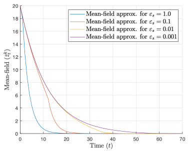
Figure 1: Mean-field approximation for different values of $\varepsilon_{s}$. Notice the convergence of the mean-field trajectory as $\varepsilon_{s}$ decreases.

Figure 2 depicts the average cost per agent for different numbers of agents, $N$ and for different values of $\varepsilon_{s}$. Each plot in the figure corresponds to a different number of agents $N$. As $N$ increases, the average cost is seen to decrease. This provides evidence that our conjecture, regarding policies obtained from the infinite population case when applied to the finite population case, is correct. The figure also shows that as the approximations become better, there is a decrease in the average cost per agent.

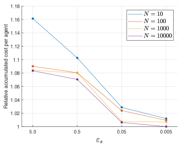
Figure 2: Relative accumulated cost per agent w.r.t. $\varepsilon_{s}$. Values are normalized to the lowest cost obtained ($N=10000$, $\varepsilon_{s}=0.005$).

VI Concluding Remarks and Future Directions

We have developed a policy iteration algorithm for approximating equilibria in infinite-horizon LQ-MFGs with discounted cost. The main challenge in the algorithm development arises from the fact that the optimal control is computed backward in time. By investigating properties of the mean-field update operator (which we term the $\tau$-latent property), we can represent the mean-field trajectory at any given iteration by a finite set of parameters, resulting in a forward-in-time construction of the optimal control. The algorithm is provably convergent, with numerical results demonstrating the nature of convergence. The optimality of the computed equilibrium has been empirically studied; naturally, the optimality of the approximate equilibrium improves as the iteration index increases and the stopping threshold decreases. The results derived in this paper provide an algorithmic viewpoint of the nature of mean-field equilibria for LQ-MFGs. We believe that such insights will be useful for developing model-free RL algorithms. Future work includes an extension to the multivariate case as well as consideration of a nonlinear/non-quadratic model (see [26]).

Proof of Lemma 1.

Substituting $K_{t}=\gamma^{t}p_{t}$ and $g_{t}=\gamma^{t}\lambda_{t}$ into (21)–(26) of [29] yields (similar derivations in [30] and on p. 234 of [31]),

$$u_{t}=-\gamma b(c_{u}+b^{2}\gamma p_{t+1})^{-1}(p_{t+1}az_{t}+\lambda_{t+1}),$$

$$\lambda_{t}=\gamma a\left(1-\gamma p_{t+1}b^{2}(c_{u}+\gamma b^{2}p_{t+1})^{-1}\right)\lambda_{t+1}-c_{z}\bar{z}_{t},$$

$$p_{t}=\gamma a^{2}p_{t+1}+c_{z}-\gamma^{2}a^{2}b^{2}p^{2}_{t+1}(c_{u}+\gamma b^{2}p_{t+1})^{-1}.$$

Since it is an infinite horizon problem, the Riccati equation will have a steady state solution. This can be written as,

$$u_{t} =-\gamma b(apz_{t}+\lambda_{t+1})/(c_{u}+\gamma b^{2}p),$$

$$p =\gamma a^{2}p+c_{z}-\gamma^{2}a^{2}b^{2}p^{2}/(c_{u}+\gamma b^{2}p),$$

$$\lambda_{t} =\gamma a\left(1-\gamma pb^{2}/(c_{u}+\gamma b^{2}p)\right)\lambda_{t+1}-c_{z}\bar{z}_{t}.$$

Defining $g_{p}:=-\gamma b/(c_{u}+\gamma b^{2}p)$ and $h_{p}:=a(1+bpg_{p})$, the above expressions for $u_{t}$ and $\lambda_{t}$ correspond to (7) and (10), respectively. Rearranging and grouping $p$ terms in the above expression yields (8), with unique positive solution (9). ∎

Proof of Lemma 2.

1) First, we show that $\gamma\lvert h_{p}\rvert<1$. It is well known [30] that the DARE for variables $(a_{c},b_{c},s_{c},r_{c})$ and average cost is $\hat{k}=a^{2}_{c}\hat{k}+s_{c}-a^{2}_{c}\hat{k}^{2}b^{2}_{c}/(r_{c}+b^{2}_{c}\hat{k})$. If $b_{c}\neq 0$ and $s_{c}>0$, then this equation will have a positive solution. Moreover, the optimal feedback gain is $l_{c}:=-a_{c}b_{c}\hat{k}/(r_{c}+b_{c}^{2}\hat{k})$ and the closed-loop gain $\lvert a_{c}+b_{c}l_{c}\rvert<1$. By using a change of variables with $a_{c}=\sqrt{\gamma}a,b_{c}=b,s_{c}=c_{z},r_{c}=c_{u}/\gamma$, the equation (8) is recovered with $\hat{k}=p$. Hence there exists a unique positive solution for (8), given by (9). Moreover $\lvert a_{c}+b_{c}l_{c}\rvert=\left\lvert\sqrt{\gamma}a-\frac{\gamma\sqrt{\gamma}ab^{2}p}{c_{u}+\gamma b^{2}p}\right\rvert=\sqrt{\gamma}\left\lvert a(1+bpg)\right\rvert=\sqrt{\gamma}\lvert h_{p}\rvert<1$ and thus $\gamma\lvert h_{p}\rvert<\sqrt{\gamma}|h_{p}|<1$. From (10), recursing backwards yields $\lambda_{0}=\left(\gamma h_{p}\right)^{t}\lambda_{t}-c_{z}\sum_{s=0}^{t-1}\left(\gamma h_{p}\right)^{s}\bar{z}_{s}$. Under the assumption $\lambda_{0}=-c_{z}\sum_{s=0}^{\infty}(\gamma h_{p})^{s}\bar{z}_{s}$, it follows that $\left(\gamma h_{p}\right)^{t}\lambda_{t}=-c_{z}\sum_{s=t}^{\infty}\left(\gamma h_{p}\right)^{s}\bar{z}_{s}\Rightarrow\lambda_{t}=-c_{z}\sum_{s=0}^{\infty}\left(\gamma h_{p}\right)^{s}\bar{z}_{t+s}$. As $\bar{z}\in\ell^{\infty}$ there exists some $0\leq\bar{z}_{\infty}<\infty$ s.t. $\lvert\bar{z}_{t}\rvert\leq\bar{z}_{\infty}$. This translates to $\lvert\lambda_{t}\rvert\leq c_{z}\bar{z}_{\infty}/(1-\gamma h_{p})$ for all $t$. Hence $\lambda\in\ell^{\infty}$.
2) The closed-loop dynamics of $z_{t}$ under the cost-minimizing control are, $z_{t+1}=az_{t}+bg_{p}(paz_{t}+\lambda_{t+1})+\omega_{t}$. Using this equation recursively, the expression for $z_{t}$ in terms of $z_{0}$ is, $z_{t}=h_{p}^{t-1}z_{0}+bg_{p}\sum^{t-1}_{s=0}h_{p}^{s}\lambda_{t-s}+\sum^{t-1}_{s=0}h_{p}^{s}\omega_{t-1-s}$. The expression for $\mathbb{E}\big{[}\big{(}z_{t}-\bar{z}_{t}\big{)}^{2}\big{]}$ is thus,

$$\mathbb{E}\big{[}\left(z_{t}-\bar{z}_{t}\right)^{2}\big{]}=\big{(}h_{p}^{t-1}\big{)}^{2}({\sigma_{0}^{2}}+\nu^{2}_{0})+\sigma_{w}^{2}\sum^{t-1}_{s=0}h_{p}^{s}+$$

$$\bigg{(}bg_{p}\sum^{t-1}_{s=0}h_{p}^{s}\lambda_{t-s}-\bar{z}_{t}\bigg{)}^{2}+2h_{p}^{t-1}\nu_{0}\bigg{(}bg_{p}\sum^{t-1}_{s=0}h_{p}^{s}\lambda_{t-s}-\bar{z}_{t}\bigg{)}.$$

Assumption 1 implies that $\lvert h_{p}\rvert<1$. Furthermore, since $\bar{z}\in\ell^{\infty}$ and $\lambda\in\ell^{\infty}$, there exist constants $\bar{z}_{\infty},\lambda_{\infty}<\infty$ such that $\bar{z}_{t}\leq\bar{z}_{\infty}$ and $\lambda_{t}\leq\lambda_{\infty}$ for all $t$. Thus,

$$\mathbb{E}\left[\left(z_{t}-\bar{z}_{t}\right)^{2}\right]\leq\left(h_{p}^{t-1}\right)^{2}(\sigma^{2}_{0}+\nu^{2}_{0})+\sigma_{w}^{2}t$$

$$+\left(bg_{p}t\lambda_{\infty}-\bar{z}_{\infty}\right)^{2}+2h_{p}^{t-1}\nu_{0}\left(bg_{p}t\lambda_{\infty}-\bar{z}_{\infty}\right).$$

Similarly, $\mathbb{E}\left[u^{2}_{t}\right]$ is bounded above as,

$$\mathbb{E}\big{[}u^{2}_{t}\big{]}=(ag_{p}p)^{2}\big{[}\big{(}h_{p}^{t-1}\big{)}^{2}\big{(}\sigma^{2}_{0}+\nu^{2}_{0}\big{)}+\sum^{t-1}_{s=0}\sigma_{w}^{2}h_{p}^{2s}$$

$$+bg_{p}h_{p}^{s}\lambda_{t-s}+2h_{p}^{t-1}\nu_{0}bg_{p}h_{p}^{s}\lambda_{t-s}\big{]}+g_{p}^{2}\lambda^{2}_{t+1}$$

$$+2ag_{p}^{2}p\lambda_{t+1}\big{(}h_{p}^{t-1}\nu_{0}+bg_{p}\sum^{t-1}_{s=0}h_{p}^{s}\lambda_{t-1}\big{)}$$

$$\leq(ag_{p}p)^{2}\left[\left(h_{p}^{t-1}\right)^{2}\left(\sigma^{2}_{0}+\nu^{2}_{0}\right)+\sigma_{w}^{2}t\right.$$

$$\left.+\left(bg_{p}t\lambda_{\infty}\right)+2h_{p}^{t-1}\nu_{0}bg_{p}t\lambda_{\infty}\right]+g_{p}^{2}\left(\lambda_{\infty}\right)^{2}$$

$$+2ag_{p}^{2}p\lambda_{\infty}\left(h_{p}^{t-1}\nu_{0}+bg_{p}t\lambda_{\infty}\right).$$

Since the optimal cost is, $\sum_{t=0}^{\infty}c_{z}\mathbb{E}\big{[}\gamma^{t}\big{(}z_{t}-\bar{z}_{t}\big{)}^{2}\big{]}+c_{u}\mathbb{E}\big{[}\gamma^{t}u^{2}_{t}\big{]}$, and $\sum_{t=0}^{\infty}t\gamma^{t}=\frac{\gamma}{(1-\gamma)^{2}},\,\sum_{t=0}^{\infty}\gamma^{t}\big{(}h_{p}^{t-1}\big{)}^{2}=\frac{1}{h_{p}^{2}\big{(}1-\gamma h_{p}^{2}\big{)}},\,\sum_{t=0}^{\infty}t\gamma^{t}h_{p}^{t-1}=\frac{\gamma}{(1-\gamma h_{p})^{2}}$ it can be concluded that the optimal cost is bounded. ∎

Proof of Lemma 3.

Let us define two mean-fields $\bar{z},\hat{z}\in\ell^{\infty}$ and their next iterates $\bar{z}^{\prime}=\mathcal{T}(\bar{z}),\hat{z}^{\prime}=\mathcal{T}(\hat{z})$. Let us define the difference sequences $\delta_{t}=\bar{z}_{t}-\hat{z}_{t}$ and $\delta^{\prime}_{t}=\bar{z}^{\prime}_{t}-\hat{z}^{\prime}_{t}$. Using (12), the equation expressing the connection between $\delta_{t}$ and $\delta^{\prime}_{t}$ is $\delta^{\prime}_{t+1}=h_{p}\delta_{t}-c_{z}bg_{p}\sum_{s=0}^{\infty}\left(\gamma h_{p}\right)^{s}\delta_{t+1+s}$. Hence,

$$\lVert\delta^{\prime}\rVert_{\infty} \leq\lVert\delta\rVert_{\infty}\Big{(}\big{\lvert}h_{p}\big{\rvert}+\Big{\lvert}c_{z}bg_{p}\sum_{s=0}^{\infty}\big{(}\gamma h_{p}\big{)}^{s}\Big{\rvert}\Big{)}$$

$$\leq\lVert\delta\rVert_{\infty}\big{(}\big{\lvert}h_{p}\big{\rvert}+\big{\lvert}c_{z}bg_{p}/(1-\gamma h_{p})\big{\rvert}\big{)}=\lVert\delta\rVert_{\infty}T_{p}$$

where the last inequality follows from $\gamma|h_{p}|<1$ (see Lemma 2). By Assumption 1, $\mathcal{T}$ is a contraction. ∎

Proof of Theorem 1.

Consider an MFE $(\mu^{*},\bar{z}^{*})$ that satisfies Definition 1. Then, by definition, $\mu^{*}=\Phi(\bar{z}^{*})$. The second part of Definition 1 states that $\bar{z}^{*}=\Lambda(\mu^{*})$. Thus $\bar{z}^{*}=\Lambda(\Phi(\bar{z}^{*}))=\mathcal{T}(\bar{z}^{*})$. Now let us prove the converse. Consider a mean-field $\bar{z}^{*}$ which is the fixed point of $\mathcal{T}$ i.e. $\bar{z}^{*}=\mathcal{T}(\bar{z}^{*})$. Then if $\mu^{*}$ is the cost-minimizing control for $\bar{z}^{*}$ i.e. $\mu^{*}=\Phi(\bar{z}^{*})$, $(\mu^{*},\bar{z}^{*})$ is an MFE since (1) $\mu^{*}=\Phi(\bar{z}^{*})$, and (2) $\Lambda(\mu^{*})=\Lambda(\Phi(\bar{z}^{*}))=\mathcal{T}(\bar{z}^{*})=\bar{z}^{*}$. ∎

Proof of Lemma 4.

For $t\in\{\tau,\tau+1,\ldots\}$ using (12) and the fact that $|r|\leq 1$, we can write $x^{\prime}_{t+1}=h_{p}x_{t}-c_{z}bg_{p}\sum_{s=0}^{\infty}\left(\gamma h_{p}r\right)^{s}rx_{t}=\hat{r}_{p}x_{t}$ where $\hat{r}_{p}:=h_{p}-\frac{c_{z}bg_{p}r}{1-\gamma h_{p}r}$. Similarly, $x^{\prime}_{t+2}$ is generated as $x^{\prime}_{t+2}=\hat{r}_{p}x_{t+1}=\hat{r}_{p}rx_{t}$ for all $t\in\{\tau,\tau+1,\ldots\}$. Grouping terms, we obtain $x^{\prime}_{t+2}=rx^{\prime}_{t+1}$ for all $t\in\{\tau,\tau+1,\ldots\}$. ∎

Proof of Theorem 2.

We first state and prove in Lemma 5 below that the expression in the stopping condition of the algorithm $\max_{0\leq t\leq k}\big{\lvert}\bar{z}^{(k)}_{t}-\bar{z}^{(k-1)}_{t}\big{\rvert}$ is equal to $\big{\lVert}\bar{z}^{(k)}-\bar{z}^{(k-1)}\big{\rVert}_{\infty}$. This is due to the fact that $\bar{z}^{(k)}$ and $\bar{z}^{(k-1)}$ both follow stable linear dynamics for $t\geq k$.

Lemma 5.

$\displaystyle\max_{0\leq t\leq k}\big{\lvert}\bar{z}^{(k)}_{t}-\bar{z}^{(k-1)}_{t}\big{\rvert}=\big{\lVert}\bar{z}^{(k)}-\bar{z}^{(k-1)}\big{\rVert}_{\infty}$.

Proof. By definition $\big{\lVert}\bar{z}^{(k)}-\bar{z}^{(k-1)}\big{\rVert}_{\infty}=\sup_{t\geq 0}\big{\lvert}\bar{z}^{(k)}_{t}-\bar{z}^{(k-1)}_{t}\big{\rvert}$. Hence for all $t\geq k$, $\big{\lvert}\bar{z}^{(k)}_{t}-\bar{z}^{(k-1)}_{t}\big{\rvert}=\big{\lvert}r^{t-k}\big{(}\bar{z}^{(k)}_{k}-\bar{z}^{(k-1)}_{k}\big{)}\big{\rvert}\leq\big{\lvert}\bar{z}^{(k)}_{k}-\bar{z}^{(k-1)}_{k}\big{\rvert}$. Using this property, $\big{\lVert}\bar{z}^{(k+1)}-\bar{z}^{(k)}\big{\rVert}_{\infty}=\sup_{t\geq 0}\big{\lvert}\bar{z}^{(k+1)}_{t}-\bar{z}^{(k)}_{t}\big{\rvert}=\max_{0\leq t\leq k+1}\big{\lvert}\bar{z}^{(k+1)}_{t}-\bar{z}^{(k)}_{t}\big{\rvert}.\hskip 40.00006pt\hfill\square$

Since $\mathcal{T}$ is contractive with a fixed point of $\bar{z}^{*}$,

$$\big{\lVert}\bar{z}^{(k+1)}-\bar{z}^{*}\big{\rVert}_{\infty}\leq T_{p}\big{\lVert}\bar{z}^{(k)}-\bar{z}^{*}\big{\rVert}_{\infty}$$ (17)

for any $k=1,2,\ldots$. The algorithm terminates at iteration $k$ when $\big{\lVert}\bar{z}^{(k+1)}-\bar{z}^{(k)}\big{\rVert}_{\infty}<\varepsilon_{s}(1-T_{p})/T_{p}$. Thus,

$$\varepsilon_{s}(1-T_{p})/T_{p} >\big{\lVert}\bar{z}^{(k+1)}-\bar{z}^{(k)}\big{\rVert}_{\infty}$$

$$\geq\big{\lVert}\bar{z}^{(k)}-\bar{z}^{*}\big{\rVert}_{\infty}-\big{\lVert}\bar{z}^{(k+1)}-\bar{z}^{*}\big{\rVert}_{\infty}$$

$$\geq\frac{1}{T_{p}}\big{\lVert}\bar{z}^{(k+1)}-\bar{z}^{*}\big{\rVert}_{\infty}-\big{\lVert}\bar{z}^{(k+1)}-\bar{z}^{*}\big{\rVert}_{\infty}$$

$$=\big{(}1-T_{p}\big{)}\big{\lVert}\bar{z}^{(k+1)}-\bar{z}^{*}\big{\rVert}_{\infty}/T_{p}.$$

Hence, $\big{\lVert}\bar{z}^{(k+1)}-\bar{z}^{*}\big{\rVert}_{\infty}<\varepsilon_{s}$ for any $\varepsilon_{s}>0$. Now we prove the bound on the number of iterations. If the number of iterations is $k>K(\varepsilon_{s})$, then,

$$k>\big{(}\log\varepsilon_{s}-\log\big{\lVert}\bar{z}^{(0)}-\bar{z}^{*}\big{\rVert}_{\infty}\big{)}/\log T_{p}$$

$$\Leftrightarrow k\log T_{p}<\log\varepsilon_{s}-\log\big{\lVert}\bar{z}^{(0)}-\bar{z}^{*}\big{\rVert}_{\infty}$$

$$\Leftrightarrow T_{p}^{k}<\frac{\varepsilon_{s}}{\big{\lVert}\bar{z}^{(0)}-\bar{z}^{*}\big{\rVert}_{\infty}}\Leftrightarrow T_{p}^{k}\big{\lVert}\bar{z}^{(0)}-\bar{z}^{*}\big{\rVert}_{\infty}<\varepsilon_{s}.$$ (18)

The inequality flip in the second step is due to the fact that $T_{p}<1$ (Assumption 1) and $\log T_{p}<0$. From (17) $\big{\lVert}\bar{z}^{(k)}-\bar{z}^{*}\big{\rVert}_{\infty}\leq T_{p}^{k}\big{\lVert}\bar{z}^{(0)}-\bar{z}^{*}\big{\rVert}_{\infty}$ and using the inequality (VI), $\big{\lVert}\bar{z}^{(k)}-\bar{z}^{*}\big{\rVert}_{\infty}<\varepsilon_{s}$.∎

References

• [1] Y. Shoham and K. Leyton-Brown, Multiagent Systems: Algorithmic, Game-theoretic, and Logical Foundations.   Cambridge University Press, 2008.
• [2] M. Wooldridge, An Introduction to Multiagent Systems.   John Wiley & Sons, 2009.
• [3] D. V. Dimarogonas, E. Frazzoli, and K. H. Johansson, “Distributed event-triggered control for multi-agent systems,” IEEE Transactions on Automatic Control, vol. 57, no. 5, pp. 1291–1297, 2011.
• [4] K. Zhang, Z. Yang, H. Liu, T. Zhang, and T. Başar, “Fully decentralized multi-agent reinforcement learning with networked agents,” in International Conference on Machine Learning, 2018, pp. 5867–5876.
• [5] K. Zhang, Z. Yang, H. Liu, T. Zhang, and T. Başar, “Finite-sample analyses for fully decentralized multi-agent reinforcement learning,” arXiv preprint arXiv:1812.02783, 2018.
• [6] R. Breban, R. Vardavas, and S. Blower, “Mean-field analysis of an inductive reasoning game: Application to influenza vaccination,” Physical Review E, vol. 76, no. 3, p. 031127, 2007.
• [7] R. Couillet, S. M. Perlaza, H. Tembine, and M. Debbah, “Electrical vehicles in the smart grid: A mean field game analysis,” IEEE Journal on Selected Areas in Communications, vol. 30, no. 6, pp. 1086–1096, 2012.
• [8] M. Huang, R. P. Malhamé, P. E. Caines et al., “Large population stochastic dynamic games: closed-loop Mckean-Vlasov systems and the Nash certainty equivalence principle,” Communications in Information & Systems, vol. 6, no. 3, pp. 221–252, 2006.
• [9] M. Huang, P. E. Caines, and R. P. Malhamé, “Individual and mass behaviour in large population stochastic wireless power control problems: Centralized and Nash equilibrium solutions,” in IEEE International Conference on Decision and Control, vol. 1.   IEEE, 2003, pp. 98–103.
• [10] J.-M. Lasry and P.-L. Lions, “Mean field games,” Japanese Journal of Mathematics, vol. 2, no. 1, pp. 229–260, 2007.
• [11] M. Huang, P. E. Caines, and R. P. Malhamé, “Large-population cost-coupled LQG problems with nonuniform agents: Individual-mass behavior and decentralized $\varepsilon$-Nash equilibria,” IEEE Transactions on Automatic Control, vol. 52, no. 9, pp. 1560–1571, 2007.
• [12] A. Bensoussan, K. Sung, S. C. P. Yam, and S.-P. Yung, “Linear-quadratic mean field games,” Journal of Optimization Theory and Applications, vol. 169, no. 2, pp. 496–529, 2016.
• [13] M. Huang and M. Zhou, “Linear quadratic mean field games–part I: The asymptotic solvability problem,” arXiv preprint arXiv:1811.00522, 2018.
• [14] J. Moon and T. Başar, “Discrete-time LQG mean field games with unreliable communication,” in 53rd IEEE Conference on Decision and Control.   IEEE, 2014, pp. 2697–2702.
• [15] J. Subramanian and A. Mahajan, “Reinforcement learning in stationary mean-field games,” in Proceedings of the 18th International Conference on Autonomous Agents and MultiAgent Systems.   International Foundation for Autonomous Agents and Multiagent Systems, 2019, pp. 251–259.
• [16] X. Guo, A. Hu, R. Xu, and J. Zhang, “Learning mean-field games,” arXiv preprint arXiv:1901.09585, 2019.
• [17] R. Elie, J. Pérolat, M. Laurière, M. Geist, and O. Pietquin, “Approximate fictitious play for mean field games,” arXiv preprint arXiv:1907.02633, 2019.
• [18] Z. Fu, Z. Yang, Y. Chen, and Z. Wang, “Actor-critic provably finds Nash equilibria of linear quadratic mean field games,” in International Conference on Learning Representations, 2020.
• [19] K. Zhang, Z. Yang, and T. Başar, “Multi-agent reinforcement learning: A selective overview of theories and algorithms,” arXiv preprint arXiv:1911.10635, 2019.
• [20] S. J. Bradtke, “Reinforcement learning applied to linear quadratic regulation,” in Advances in Neural Information Processing Systems, 1993, pp. 295–302.
• [21] M. Fazel, R. Ge, S. M. Kakade, and M. Mesbahi, “Global convergence of policy gradient methods for the linear quadratic regulator,” in International Conference on Machine Learning, 2018, pp. 1467–1476.
• [22] K. Zhang, Z. Yang, and T. Başar, “Policy optimization provably converges to Nash equilibria in zero-sum linear quadratic games,” in Advances in Neural Information Processing Systems, 2019.
• [23] B. Kiumarsi, F. L. Lewis, H. Modares, A. Karimpour, and M.-B. Naghibi-Sistani, “Reinforcement Q-learning for optimal tracking control of linear discrete-time systems with unknown dynamics,” Automatica, vol. 50, no. 4, pp. 1167–1175, 2014.
• [24] H. Modares and F. L. Lewis, “Linear quadratic tracking control of partially-unknown continuous-time systems using reinforcement learning,” IEEE Transactions on Automatic control, vol. 59, no. 11, pp. 3051–3056, 2014.
• [25] P. Cardaliaguet and C.-A. Lehalle, “Mean field game of controls and an application to trade crowding,” Mathematics and Financial Economics, vol. 12, no. 3, pp. 335–363, 2018.
• [26] N. Saldi, T. Başar, and M. Raginsky, “Markov–Nash equilibria in mean-field games with discounted cost,” SIAM Journal on Control and Optimization, vol. 56, no. 6, pp. 4256–4287, 2018.
• [27] M. Huang, “Stochastic control for distributed systems with applications to wireless communications,” Ph.D. dissertation, McGill University, 2003.
• [28] D. G. Luenberger, Optimization by Vector Space Methods.   John Wiley & Sons, 1997.
• [29] K. Yazdani and M. Hale, “Technical report: Infinite horizon discrete-time linear quadratic Gaussian tracking control derivation,” arXiv preprint arXiv:1807.04700, 2018.
• [30] D. P. Bertsekas, Dynamic Programming and Optimal Control.   Athena scientific Belmont, MA, 1995, vol. 1, no. 2.
• [31] T. Başar and G. J. Olsder, Dynamic Noncooperative Game Theory.   Siam, 1999, vol. 23.