Brownian heat engine with active reservoirs

Abstract

Microorganisms such as bacteria are active matters which consume chemical energy and generate their unique run-and-tumble motion. A swarm of such microorganisms provide a nonequilibrium active environment whose noise characteristics are different from those of thermal equilibrium reservoirs. One important difference is a finite persistence time, which is considerably large compared to that of the equilibrium noise, that is, the active noise is colored. Here, we study a mesoscopic energy-harvesting device (engine) with active reservoirs harnessing this noise nature. For a simple linear model, we analytically show that the engine efficiency can surpass the conventional Carnot bound, thus the power-efficiency tradeoff constraint is released, and the efficiency at the maximum power can overcome the Curzon-Ahlborn efficiency. We find that the supremacy of the active engine critically depends on the time-scale symmetry of two active reservoirs.

Introduction – Mounting social need on sustainable development has attracted a great attention on energy harvesting techniques, by which useful energy is extracted from surrounding environments, in both scientific and engineering societies energy_harvest_review1 ; energy_harvest_review2 ; graphene . Typical examples are thermoelectric devices using a temperature gradient harvesting_thermoelectric , photovoltaic devices using sunlights harvesting_photo , and piezoelectric devices using ambient pressure harvesting_piezo . A major challenging issue on these studies is achieving a high efficiency as well as a high energy or power production. When a device works in an equilibrium environment, the efficiency is bound by the thermodynamic second law; for example, the efficiency of thermoelectric devices cannot surpass the Carnot efficiency.

Then, how is the efficiency affected by replacing the environment with nonequilibrium reservoirs? One might think that the efficiency would be reduced with nonequilibrium reservoirs as the efficiency usually diminishes with irreversibility. However, this is not always true: It was already reported that the efficiency of a quantum heat engine can surpass the conventional Carnot limit with nonequilibrium squeezed reservoirs squeezed1 ; squeezed2 ; squeezed3 . In classical systems, it was experimentally shown that the efficiency of a Stirling engine working in a bacterial bath can overcome its maximum efficiency obtained by a quasistatic operation in equilibrium reservoirs bacterial_bath_exp ; wijland . In addition, there are also a few examples where the efficiency increases with the irreversibility in well-manipulated ways JSLee1 ; JSLee2 ; PoEs . However, a systematic study on the efficiency bound of engines working in nonequilibrium environments has rarely been done, partly because its theoretical manipulation is not straightforward as in the equilibrium cases.

In this work, we study the efficiency and the power of an energy-harvesting device extracting energy from nonequilibrium active reservoirs. To be specific, we consider an overdamped Brownian motion of passive particles composing of the engine with equilibrium baths and/or bacterial active baths. A bacterial bath is known to be well described by the colored noise with a finite persistence time scale bacteria_exp1 ; bacteria_exp2 ; bacteria_exp3 ; bacteria_exp4 ; Bechinger ; Dabelow . In the case with the active baths, we demonstrate rigorously that (i) the efficiency can surpass the standard Carnot limit, thus the conventional power-efficiency tradeoff relation power-eff-rel1 ; power-eff-rel2 ; power-eff-rel3 does not hold and (ii) the efficiency at the maximum power (EMP) can overcome the Curzon-Ahlborn (CA) efficiency CAefficiency . We also find that the supremacy of the active engine is achieved when the time scales of the two active baths are different from each other.

Engine with equilibrium reservoirs – We first revisit the simple linear Brownian engine model with equilibrium reservoirs in the overdamped limit Crisanti ; ParkJM . Suppose that there are two particles (particle $1$ and $2$), each of which moves in a one-dimensional space and is immersed in a heat reservoir with temperature $T_{i}$ ($i=1,2$). Their positions are denoted by $x_{1}$ and $x_{2}$ and $\Phi=\Phi(x_{1},x_{2})$ is a given potential. The motions of these particles are described by the following equations:

$$\gamma_{i}\dot{x}_{i}=-\partial_{x_{1}}\Phi+f_{i}^{\textrm{nc}}+\sqrt{2k_{\textrm{B}}\gamma_{i}T_{i}}\xi_{i}~{},$$ (1)

where $\gamma_{i}$ is a dissipation coefficient, $f_{i}^{\textrm{nc}}$ is an external nonconservative force, and $k_{\textrm{B}}$ is the Boltzmann constant, which will be set to $1$ in the following discussion. $\xi_{i}$ is a Gaussian white noise satisfying $\langle\xi_{i}(t)\rangle=0$ and $\langle\xi_{i}(t)\xi_{j}(t^{\prime})\rangle=\delta_{ij}\delta(t-t^{\prime})$. In this model, the harmonic potential and the linear nonconservative force are taken for analytic treatments ParkJM ; Chulan ; Pietzonka ; Chun as

$$\Phi=\frac{k}{2}(x_{1}^{2}+x_{2}^{2})~{},\quad(f_{1}^{\textrm{nc}},f_{2}^{\textrm{nc}})=(\epsilon x_{2},\delta x_{1})~{}.$$ (2)

Note that the Brownian gyrator Filliger has a similar structure, which was experimentally realized recently Chiang .

From Eq. (1), the thermodynamic first law can be written as

$$\dot{Q}_{i}=\dot{E}_{i}+\dot{W}_{i}~{},$$ (3)

where $\dot{E}_{i}=\dot{x}_{i}\partial_{x_{i}}\Phi$ is the rate of the internal energy change of a particle $i$, $\dot{W}_{i}=-f_{i}^{\textrm{nc}}\dot{x}_{i}$ is the work extraction rate due to the external force $f_{i}^{\textrm{nc}}$, and $\dot{Q}_{i}=\dot{x}_{i}\circ(-\gamma_{i}\dot{x}_{i}+\sqrt{2\gamma_{i}T_{i}}\xi_{i})$ is the heat current out of the bath $i$ with the Stratonovich multiplication denoted by $\circ$ Risken . In the steady state, $\langle\dot{Q}_{i}\rangle_{\textrm{s}}=\langle\dot{W}_{i}\rangle_{\textrm{s}}$ as $\langle\dot{E}_{i}\rangle_{\textrm{s}}=0$, where $\langle\cdots\rangle_{\textrm{s}}$ denotes the steady-state average. Therefore, $\langle\dot{Q}_{1}\rangle_{\textrm{s}}=-\epsilon\langle x_{2}\dot{x}_{1}\rangle_{\textrm{s}}$ and $\langle\dot{Q}_{2}\rangle_{\textrm{s}}=-\delta\langle x_{1}\dot{x}_{2}\rangle_{\textrm{s}}$. The total work rate (power) is $\langle\dot{W}\rangle_{\textrm{s}}=\langle\dot{W}_{1}\rangle_{\textrm{s}}+\langle\dot{W}_{2}\rangle_{\textrm{s}}=(\epsilon-\delta)\langle x_{1}\dot{x}_{2}\rangle_{\textrm{s}}$, where the second equality comes from the fact $\frac{d}{dt}\langle x_{1}x_{2}\rangle_{\textrm{s}}=\langle\dot{x}_{1}x_{2}\rangle_{\textrm{s}}+\langle x_{1}\dot{x}_{2}\rangle_{\textrm{s}}=0$.

For $T_{1}>T_{2}$, the efficiency $\eta$ is given by the ratio between $\langle\dot{W}\rangle_{\textrm{s}}$ and $\langle\dot{Q}_{1}\rangle_{\textrm{s}}$ as

$$\eta=\frac{\langle\dot{W}\rangle_{\textrm{s}}}{\langle\dot{Q}_{1}\rangle_{\textrm{s}}}=1-\frac{\delta}{\epsilon}~{}.$$ (4)

Requiring the work extraction $\langle\dot{W}\rangle_{\textrm{s}}=(\epsilon-\delta)\langle x_{1}\dot{x}_{2}\rangle_{\textrm{s}}\geq 0$ with

$$\langle x_{1}\dot{x}_{2}\rangle_{\textrm{s}}=\frac{T_{1}\delta-T_{2}\epsilon}{k(\gamma_{1}+\gamma_{2})}~{},$$ (5)

we find the constraint $T_{2}/T_{1}\leq\delta/\epsilon\leq 1$, leading to the famous Carnot bound as

$$0\leq\eta\leq 1-\frac{T_{2}}{T_{1}}\equiv\eta_{\textrm{C}}~{},$$ (6)

where $\eta_{\textrm{C}}$ is the Carnot efficiency. As expected from the power-efficiency tradeoff relation, the power $\langle\dot{W}\rangle_{\textrm{s}}$ vanishes at $\eta=\eta_{\textrm{C}}$ power-eff-rel1 ; power-eff-rel2 ; power-eff-rel3 . In addition, we need the stability condition for the existence of the steady state, which turns out to be

$$\delta\epsilon\equiv K<k^{2}~{}.$$ (7)

Derivations of Eqs. (5) and (7) are presented in Supplemental Material (SM) I.A.

Figure 1(a) shows the engine area satisfying the above two constraints (6) and (7) with $\gamma_{1}=\gamma_{2}=1$, $k=2$, $T_{1}=2$, and $T_{2}=1$. In Fig. 1(b), we plot the normalized efficiency and power as $\tilde{\eta}\equiv\eta/\eta_{\textrm{C}}$ and $\tilde{P}\equiv\langle\dot{W}\rangle_{\textrm{s}}/P_{\textrm{eq}}^{\textrm{max}}$ along the line from $\epsilon_{1}$ to $\epsilon_{2}$ of Fig. 1(a) at fixed $\delta=0.8$, where $P_{\textrm{eq}}^{\textrm{max}}$ is the maximum power in equilibrium baths defined as Eq. (8). Note that the solid curves and data points of Fig. 1 are analytic curves and numerical simulation results, respectively. All numerical data are obtained by integrating the equations of motion of Eq. (1) and averaging over $2\times 10^{6}$ samples in the steady state.

We also calculate the efficiency at the maximum power (EMP) $\eta_{\textrm{EMP}}$. Along the curve with fixed $K$ $(0\leq K\leq k^{2})$, the local maximum power is obtained at $\delta_{\textrm{m}}=\sqrt{T_{2}/T_{1}}\epsilon_{\textrm{m}}$ with the efficiency $\eta_{\textrm{m}}$ identical to the Curzon-Ahlborn (CA) efficiency $\eta_{\textrm{CA}}$ CAefficiency and the power given by $\langle\dot{W}\rangle_{\textrm{s}}^{\textrm{m}}=KT_{1}\eta_{\textrm{CA}}^{2}/k(\gamma_{1}+\gamma_{2})$. The global power maximum is achieved at $K=k^{2}$, thus we obtain

$$\eta_{\textrm{EMP}}=1-\sqrt{\frac{T_{2}}{T_{1}}}\equiv\eta_{\textrm{CA}}~{}~{}~{}\textrm{and}~{}~{}P_{\textrm{eq}}^{\textrm{max}}\equiv\frac{kT_{1}\eta_{\textrm{CA}}^{2}}{\gamma_{1}+\gamma_{2}}~{}.$$ (8)

Figure 1(c) shows the plots of $\tilde{\eta}_{\textrm{m}}\equiv\eta_{\textrm{m}}/\eta_{\textrm{CA}}$ and $\tilde{P}_{\textrm{m}}\equiv\langle\dot{W}\rangle_{\textrm{s}}^{\textrm{m}}/P_{\textrm{eq}}^{\textrm{max}}$ against $K$.

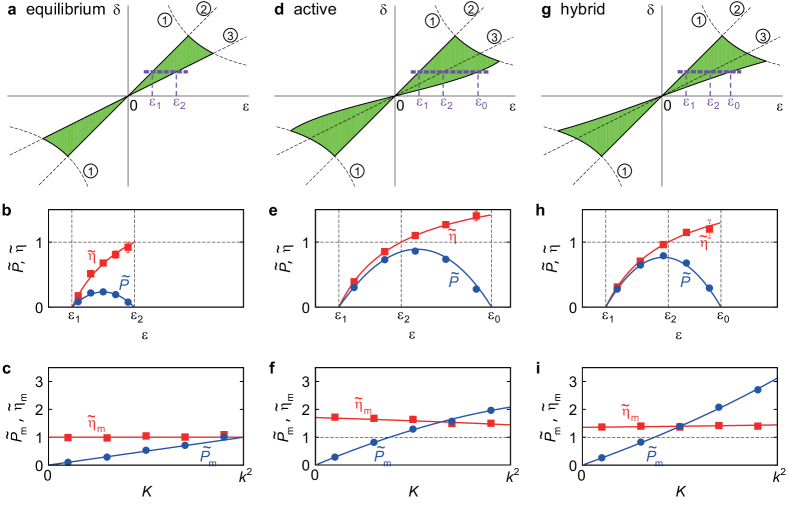
Figure 1: Performance of the engine in various environments. Shaded areas in (a), (d), and (g) denote the areas in which the device works as a stable and useful engine for equilibrium, active, and hybrid reservoirs, respectively. \scriptsize1⃝, \scriptsize2⃝, and \scriptsize3⃝ denote the curves $\epsilon\delta=k^{2}$, $\delta=\epsilon$, and $\delta=\epsilon T_{2}/T_{1}$ or $\delta=\epsilon T_{2}^{\textrm{e}}/T_{1}^{\textrm{e}}$, respectively. (b), (e), and (h) show the plots of $\tilde{\eta}\equiv\eta/\eta_{\textrm{C}}$ or $\tilde{\eta}\equiv\eta/\eta_{\textrm{C}}^{\textrm{e}}$ and $\tilde{P}\equiv\langle\dot{W}\rangle_{\textrm{s}}/P_{\textrm{eq}}^{\textrm{max}}$ along the thick dashed line of (a), (d), and (g) from $\epsilon_{1}$ to $\epsilon_{2}$ or $\epsilon_{0}$ at fixed $\delta=0.8$, respectively. The efficiency for the active and the hybrid bath can surpass the effective Carnot efficiency $\eta_{\textrm{C}}^{\textrm{e}}$ while the efficiency of the equilibrium bath is bounded by the conventional $\eta_{\textrm{C}}$. Solid curves and data points indicate analytic and numerical results, respectively. (c), (f), and (i) show the plots of $\tilde{\eta}_{\textrm{m}}\equiv\eta_{\textrm{m}}/\eta_{\textrm{CA}}$ or $\tilde{\eta}_{\textrm{m}}\equiv\eta_{\textrm{m}}/\eta_{\textrm{CA}}^{\textrm{e}}$ and $\tilde{P}_{\textrm{m}}\equiv\langle\dot{W}\rangle_{\textrm{s}}^{\textrm{m}}/P_{\textrm{eq}}^{\textrm{max}}$ against $K(=\delta\epsilon)$. The EMP for the active and the hybrid bath surpass $\eta_{\textrm{CA}}^{\textrm{e}}$. The maximum power also become larger for the active and the hybrid baths than that for the equilibrium bath.

Engine with active reservoirs – Now, we replace equilibrium reservoirs with bacterial active baths. The equations of motion are given as

$$\gamma_{i}\dot{x}_{i} =-\partial_{x_{i}}\Phi+f_{i}^{\textrm{nc}}+\zeta_{i}~{}.$$ (9)

Here, $\zeta_{i}$ is a Gaussian colored noise satisfying $\langle\zeta_{i}(t)\zeta_{j}(t^{\prime})\rangle=D_{i}\delta_{ij}e^{-|t-t^{\prime}|/\tau_{i}}/\tau_{i}$, where $D_{i}$ is the noise strength and $\tau_{i}$ is the persistence time scale of noise $\zeta_{i}$ bacteria_exp1 ; bacteria_exp2 ; bacteria_exp3 ; bacteria_exp4 ; Bechinger ; Dabelow . The finite persistent time originates from collisions of a passive particle with bacteria with directional persistence. In the $\tau_{i}\rightarrow 0$ limit, the active bath becomes identical to the equilibrium bath with the temperature $T_{i}=D_{i}/\gamma_{i}$. The Ornstein-Uhlenbeck process (OUP) provides one of the simplest ways to describe the evolution of $\zeta_{i}$ Risken :

$$\tau_{i}\dot{\zeta}_{i}=-\zeta_{i}+\sqrt{2D_{i}}\xi_{i}~{},$$ (10)

where $\xi_{i}$ is a Gaussian white noise as seen in Eq. (1). Together with Eq. (9), this process with linear forces like in Eq. (2) is called the active OUP (AOUP) Fodor ; Madal ; Marconi ; Dabelow . We remark that a non-Gaussian nature of the colored noise was observed experimentally in a low-concentration bacterial bath bacteria_exp3 . However, our results in the following can also apply to a non-Gaussian case because the work and heat current in the linear-force system do not depend on the higher-order moments of the noise except for the second-order one wijland .

Before investigating the AOUP engine, we first consider passive particles trapped in a harmonic potential in Eq. (2) without a nonconservative force ($f_{i}^{\textrm{nc}}=0$), in contact with the active reservoir. From its steady state distribution, we can unambiguously define the appropriate effective temperature of the active reservoir as follows. It is straightforward (see SM I.B) to derive the steady state distribution which is Boltzmannlike in this case as

$$P(x_{1},x_{2})=\prod_{i=1}^{2}\sqrt{\frac{k}{2\pi{T}_{i}^{\textrm{e}}}}e^{-\frac{kx_{i}^{2}}{2{T}_{i}^{\textrm{e}}}},$$ (11)

where the effective temperature ${T}_{i}^{\textrm{e}}\equiv D_{i}/\Gamma_{i}$ with $\Gamma_{i}=\gamma_{i}+k\tau_{i}$. Note that ${T}_{i}^{\textrm{e}}\leq D_{i}/\gamma_{i}=T_{i}$ and depends not only on the persistent time $\tau_{i}$ but also on the stiffness $k$ of the harmonic potential. It is not surprising to see the effectively lower temperature because the persistence reduces the stochasticity.

The energy conservation yields again Eq. (3) where the heat current out of the active bath $i$ is given by $\dot{Q}_{i}=\dot{x}_{i}\circ(-\gamma_{i}\dot{x}_{i}+\zeta_{i})$. In the steady state for the AOUP engine, we get the same form as before for the heats and power such as $\langle\dot{Q}_{1}\rangle_{\textrm{s}}=\langle\dot{W}_{1}\rangle_{\textrm{s}}=\epsilon\langle x_{1}\dot{x}_{2}\rangle_{\textrm{s}}$ and $\langle\dot{W}\rangle_{\textrm{s}}=(\epsilon-\delta)\langle x_{1}\dot{x}_{2}\rangle_{\textrm{s}}$. The standard calculation of the multivariate OUP Risken by treating the colored noise $\zeta_{i}$ as a state variable yields (see SM I.C)

$$\langle x_{1}\dot{x}_{2}\rangle_{\textrm{s}}=\frac{1}{k(\gamma_{1}+\gamma_{2})}\left[\frac{T_{1}^{\textrm{e}}\delta}{\mathcal{A}_{K}}-\frac{T_{2}^{\textrm{e}}\epsilon}{\mathcal{B}_{K}}\right]\quad\textrm{with}~{}~{}K=\delta\epsilon~{},$$ (12)

where

$$\mathcal{A}_{K} =1+\frac{k\gamma_{1}\tau_{1}}{\gamma_{2}\Gamma_{1}}+\frac{(k^{2}-K)\tau_{1}^{2}}{\gamma_{2}\Gamma_{1}}~{},$$

$$\mathcal{B}_{K} =1+\frac{k\gamma_{2}\tau_{2}}{\gamma_{1}\Gamma_{2}}+\frac{(k^{2}-K)\tau_{2}^{2}}{\gamma_{1}\Gamma_{2}}~{}.$$ (13)

We find the same stability condition ($K<k^{2}$, see SM I.C), thus $\mathcal{A}_{K}\geq 1$ and $\mathcal{B}_{K}\geq 1$ in the stable region.

With the same definition of the efficiency for a passive engine in Eq. (4) (see further discussions in SM II), we find the efficiency bound from the engine condition as

$$0\leq\eta=1-\frac{\delta}{\epsilon}\leq 1-\frac{T_{2}^{\textrm{e}}\mathcal{A}_{K}}{T_{1}^{\textrm{e}}\mathcal{B}_{K}}\equiv\eta_{\textrm{C}}^{\textrm{a}}~{},$$ (14)

where $\eta_{\textrm{C}}^{\textrm{a}}$ is the maximum efficiency for the AOUP engine. It is remarkable to see that $\eta_{\textrm{C}}^{\textrm{a}}$ can exceed the effective Carnot efficiency $\eta_{\textrm{C}}^{\textrm{e}}=1-{T_{2}^{\textrm{e}}}/{T_{1}^{\textrm{e}}}$ when the modification factor $\mathcal{M}_{K}\equiv\mathcal{B}_{K}/\mathcal{A}_{K}>1$. The modification factor $\mathcal{M}_{K}$ is maximized and reaches $1+k\tau_{2}/\gamma_{1}$ in the limits of $\tau_{1}/\tau_{2}\rightarrow 0$ and $K\rightarrow 0$.

The case with the time-scale symmetry ($\tau_{1}=\tau_{2}$ and $\gamma_{1}=\gamma_{2}$) is special. We get $\mathcal{M}_{K}=1$ and $T_{2}^{\textrm{e}}/T_{1}^{\textrm{e}}=T_{2}/T_{1}$, thus $\eta_{\textrm{C}}^{\textrm{a}}=1-T_{2}/T_{1}=\eta_{\textrm{C}}$; no effect on the efficiency but the power is reduced by a factor of $\mathcal{A}_{K}(1+k\tau_{1}/\gamma_{1})\geq 1$. Therefore, the breaking of the time-scale symmetry is crucial in enhancing the engine performance. Similar phenomena were found recently in some quantum engines Cao ; Um , where the quantum-ness disappears with the symmetry.

Furthermore, we can see that the active engine can do work with two active reservoirs with the same effective temperatures, but with different persistence times. This also manifests that the active reservoir should be characterised not only by its effective temperature but also by its persistent time. More remarkably, the heat flows can be reversed ($\langle\dot{Q}_{1}\rangle_{\textrm{s}}<0$, $\langle\dot{Q}_{2}\rangle_{\textrm{s}}>0$ for $T_{1}^{\textrm{e}}\geq T_{2}^{\textrm{e}}$), still with the positive work extraction $\langle\dot{W}\rangle_{\textrm{s}}>0$) when $T_{2}^{\textrm{e}}/\mathcal{B}_{K}>T_{1}^{\textrm{e}}/\mathcal{A}_{K}$ (see detailed discussions in SM I.C).

To illustrate the enhancement of the active engine performance, we consider a simple case with $\tau_{1}=0$ (high-temperature equilibrium reservoir) and $\tau_{2}>0$ (low-temperature active reservoir). Then, it is clear that $\eta_{\textrm{C}}^{\textrm{a}}$ is always larger than $\eta_{\textrm{C}}^{\textrm{e}}$ as $\mathcal{A}_{K}=1$ and $\mathcal{B}_{K}>1$. Furthermore, as $T_{1}^{\textrm{e}}=T_{1}$ and $T_{2}^{\textrm{e}}=T_{2}/(1+k\tau_{2}/\gamma_{2})<T_{2}$, we find $\eta_{\textrm{C}}^{\textrm{a}}>\eta_{\textrm{C}}^{\textrm{e}}>\eta_{\textrm{C}}$. From Eq. (12), we can also easily see that the power is enhanced in this case, compared to the case of both equilibrium reservoirs ($\tau_{1}=\tau_{2}=0$).

Figure 1(d) shows the region satisfying the stable and useful engine condition with $\tau_{1}=0$, $\tau_{2}=0.5$, $T_{1}^{\textrm{e}}=2$, and $T_{2}^{\textrm{e}}=1$, which is extended outside of the line of $\delta=(T_{2}^{\textrm{e}}/T_{1}^{\textrm{e}})\epsilon$, where the efficiency $\eta$ is larger than $\eta_{\textrm{C}}^{\textrm{e}}$. The boundary of the extended region is given by $\langle x_{1}\dot{x}_{2}\rangle_{\textrm{s}}=0$ in Eq. (12), thus in this case, $\delta=(T_{2}^{\textrm{e}}/(\mathcal{B}_{K}T_{1}^{\textrm{e}}))\epsilon$, which is not a straight line because of $K=\delta\epsilon$. In Fig. 1(e), the normalized efficiency and power as $\tilde{\eta}\equiv\eta/\eta_{\textrm{C}}^{\textrm{e}}$ and $\tilde{P}\equiv\langle\dot{W}\rangle_{\textrm{s}}/P_{\textrm{eq}}^{\textrm{max}}$ along the thick dashed line from $\epsilon_{1}$ to $\epsilon_{0}$ of Fig. 1(d) are plotted at fixed $\delta=0.8$, where $\epsilon_{0}$ is the largest point allowed in the engine region. The efficiency clearly exceeds the effective Carnot efficiency by far and the power is finite even at the effective Carnot efficiency. This shows that the conventional power-efficiency tradeoff constraint power-eff-rel1 ; power-eff-rel2 ; power-eff-rel3 is not valid in the active engine.

We also show that the EMP of this AOUP engine can surpasses the CA efficiency. Along the curve with fixed $K$, the local maximum power is obtained at $\delta_{\textrm{m}}=\sqrt{T_{2}^{\textrm{e}}/(\mathcal{B}_{K}T_{1}^{\textrm{e}})}\epsilon_{\textrm{m}}$ with the efficiency and the power

$$\eta_{\textrm{m}}=1-\sqrt{\frac{T_{2}^{\textrm{e}}}{\mathcal{B}_{K}T_{1}^{\textrm{e}}}}>\eta_{\textrm{CA}}^{\textrm{e}}~{}~{}~{}\textrm{and}~{}~{}\langle\dot{W}\rangle_{\textrm{s}}^{\textrm{m}}\equiv\frac{KT_{1}^{\textrm{e}}\eta_{\textrm{m}}^{2}}{k(\gamma_{1}+\gamma_{2})},$$ (15)

where $\eta_{\textrm{CA}}^{\textrm{e}}\equiv 1-\sqrt{T_{2}^{\textrm{e}}/T_{1}^{\textrm{e}}}$ is the effective CA efficiency. The global power maximum is achieved at a nontrivial value of $K$ for $0\leq K\leq k^{2}$ and $\eta_{\textrm{EMP}}$ exceeds $\eta_{\textrm{CA}}^{\textrm{e}}$. Figure 1(f) shows the plots of $\tilde{\eta}_{\textrm{m}}\equiv\eta_{\textrm{m}}/\eta_{\textrm{CA}}^{\textrm{e}}$ and $\tilde{P}_{\textrm{m}}\equiv\langle\dot{W}\rangle_{\textrm{s}}^{\textrm{m}}/P_{\textrm{eq}}^{\textrm{max}}$ against $K$. Note that the dependence of $\eta_{C}^{\textrm{a}}$ and $\langle\dot{W}\rangle_{\textrm{s}}^{\textrm{m}}$ on general $\tau_{1}$ and $\tau_{2}$ is presented in SM III.

In the above example, it is easy to understand why the efficiency $\eta$ can be larger than $\eta_{\textrm{C}}$: This is simply because $T_{2}^{\textrm{e}}<T_{2}$ which provides effectively the bigger temperature gradient. However, there is a nontrivial additional enhancement of the engine performance, which is encoded in the modification factor $\mathcal{M}_{K}$. In order to understand this remarkable effect, it is useful to resort to a different representation of the equations of motion of the active engine as follows.

It is well known that the AOUP can be mapped on an underdamped Langevin dynamics by introducing an auxiliary velocity $v_{i}\equiv\dot{x}_{i}$ and mass $m_{i}\equiv\gamma_{i}\tau_{i}$ as follows Fodor ; Marconi ; Madal :

$$\dot{x}_{1} =v_{1},~{}~{}m_{1}\dot{v}_{1}=-kx_{1}+\epsilon x_{2}+\tau_{1}\epsilon v_{2}-\Gamma_{1}v_{1}+\sqrt{2D_{1}}\xi_{1}~{},$$

$$\dot{x}_{2} =v_{2},~{}~{}m_{2}\dot{v}_{2}=-kx_{2}+\delta x_{1}+\tau_{2}\delta v_{1}-\Gamma_{2}v_{2}+\sqrt{2D_{2}}\xi_{2}~{},$$ (16)

which describes the dynamics of a particle in a harmonic trap with the nonconservative force $f_{i}^{\textrm{nc}}$ and the unusual non-antisymmetric Lorentz-like velocity-dependent force $(\tau_{1}\epsilon v_{2},\tau_{2}\delta v_{1})$ in contact with the equilibrium reservoirs with the temperature ${T}_{i}^{\textrm{e}}=D_{i}/\Gamma_{i}$. The standard antisymmetric Lorenz force such as a magnetic force does not do work by itself. However, the non-antisymmetric Lorentz-like force can do work as well as change the steady-state distribution function in a significant way. Thus, the existence of the velocity-dependent force can promote the work rate as well as the heat rate, which makes it possible to exceed the effective Carnot efficiency. Note that the heat flow out of the active reservoir in this representation is given as $\dot{Q}_{1}^{\textrm{a}}=v_{1}\circ(\tau_{1}\epsilon v_{2}-\Gamma_{1}v_{1}+\sqrt{2D_{1}}\xi_{1})$ and similarly for $\dot{Q}_{2}^{\textrm{a}}$, of which the steady-state averages are identical to the heat rates $\langle\dot{Q}_{1}\rangle_{s}$ and $\langle\dot{Q}_{1}\rangle_{s}$ calculated previously.

It is also useful to study the entropy production (EP) or irreversibility for the active engine. Some years ago, Zamponi et al. showed that the stochastic thermodynamic approach for the EP can be generalized to a non-Markovian process with a memory kernel Zamponi . Very recently, the EP for the AOUP was explicitly derived using this method, which turns out to be equivalent to the EP obtained for the above auxiliary underdamped dynamics with the standard definition of the parity Fodor ; Caprini1 ; Caprini2 . Furthermore, the EP calculation method in an underdamped dynamics with general velocity-dependent forces is well documented Kwon ; Lee_old . In this study, we take this latter approach to derive the EP for the AOUP engine exactly and show that the unconventional EP term appearing generally with velocity-dependent forces plays a key role, which provides the main source for the efficiency surpassing the Carnot efficiency in the EP perspective (see SM IV).

Engine with hybrid reservoirs – Finally, we consider a more realistic hybrid engine by adding active particles (bacteria) into equilibrium fluid reservoirs bacteria_exp4 ; Bechinger ; Dabelow ; Caprini2 . Then, the equations of motion are given by

$$\gamma_{i}\dot{x}_{i}=-\partial_{x_{i}}\Phi+f_{i}^{\textrm{nc}}+\zeta_{i}+\sqrt{2\gamma_{i}T_{i}}\xi_{i}^{\prime}~{},$$ (17)

where the reservoir noise is composed of two independent noises: a Gaussian white noise $\xi_{i}^{\prime}$ with $\langle\xi_{i}^{\prime}(t)\xi_{j}^{\prime}(t^{\prime})\rangle=\delta_{ij}\delta(t-t^{\prime})$ and a Gaussian colored noise $\zeta_{i}$ with $\langle\zeta_{i}(t)\zeta_{j}(t^{\prime})\rangle=D_{i}\delta_{ij}e^{-|t-t^{\prime}|/\tau_{i}}/\tau_{i}$. Equation (17) can also describe the dynamics of a self-propelled particle as an engine particle with equilibrium baths hybrid .

In the steady state, the power and heat rates are expressed in the same form as before, e.g. $\langle\dot{W}\rangle_{\textrm{s}}=(\epsilon-\delta)\langle x_{1}\dot{x}_{2}\rangle_{\textrm{s}}$. Following the previous calculation procedure, we find (see SM I.D)

$$\langle x_{1}\dot{x}_{2}\rangle_{\textrm{s}}=\frac{T_{1}\delta-T_{2}\epsilon}{k(\gamma_{1}+\gamma_{2})}+\frac{1}{k(\gamma_{1}+\gamma_{2})}\left(\frac{D_{1}\delta}{\Gamma_{1}\mathcal{A}_{K}}-\frac{D_{2}\epsilon}{\Gamma_{2}\mathcal{B}_{K}}\right)~{},$$ (18)

which is a simple sum of two currents due to equilibrium noises and active noises. Note that the power can be enhanced (or reduced) by adding the active noise into the high-temperature (low-temperature) reservoir. In Figs. 1(g), (h), and (i), we plot the engine region, the power, the efficiency with the parameters $\tau_{1}=0.5$, $\tau_{2}=0$, $T_{1}=2$, $T_{2}=1$ $D_{1}=3$, and $D_{2}=0$. We also obtain the effective temperature of the hybrid reservoir as ${T}_{i}^{\textrm{e}}=T_{i}+D_{i}/\Gamma_{i}$ (see SM I.B), and then the engine condition yields

$$0\leq\eta\leq 1-\frac{T_{2}^{\textrm{e}}+T_{2}(\mathcal{B}_{K}-1)}{T_{1}^{\textrm{e}}+T_{1}(\mathcal{A}_{K}-1)}\left(\frac{\mathcal{A}_{K}}{\mathcal{B}_{K}}\right)\equiv\eta_{\textrm{C}}^{hybrid}~{},$$ (19)

with the maximum efficiency $\eta_{\textrm{C}}^{hybrid}$ which can again exceed the effective Carnot efficiency $\eta_{\textrm{C}}^{\textrm{e}}$. The EMP and the maximum power can be also derived.

Conclusion – We demonstrated that the power and the efficiency of a device working in nonequilibrium active environments with Gaussian colored noises with finite persistent time can overcome the conventional Carnot limit. This is possible because the total EP in the steady state cannot be expressed solely by the Clausius EP, and the unconventional EP term Kwon ; Lee_old emerges due to a velocity-dependent force present in the underdamped representation. In fact, the Clausius EP is negative for overcoming the Carnot bound, which is compensated by the positive contribution from the unconventional EP. This gives rise to the non-negative total EP, which is fully consistent with the thermodynamic second law.

We note that our main results should be also applied to more general cases with non-Gaussian colored noises. This implies that the non-Markovianity of the active noise is more crucial than its non-Gaussianity for the out-performance of the active engine, in contrast to the recent claim by Krishnamurthy et al. bacterial_bath_exp . Furthermore, we find that the time-scale symmetry breaking between two active reservoirs is necessary for the supremacy of the active engine.

Our result is readily realizable and applicable to the energy harvesting devices in bacterial or active baths. Thus, our conclusion provides a new way of developing high-performance energy-harvesting devices harnessing energy of microorganisms which exist almost everywhere in nature.

- (1) R.J.M. Vullers, R. van Schaijk, I. Doms, C. Van Hoof, R. Mertens, Micropower energy harvesting, Solid-State Electronics 53, 684–693 (2009).
- (2) L. Mateu and F. Moll, Review of energy harvesting techniques and applications for microelectronics (Keynote Address), Proc. SPIE 5837, VLSI Circuits and Systems II, (2005).
- (3) P. M. Thibado, P. Kumar, S. Singh, M. Ruiz-Garcia, A. Lasanta, and L. L. Bonilla, Fluctuation-induced current from freestanding graphene: toward nanoscale energy harvesting, e-print arXiv:2002.09947.
- (4) M. Josefsson, A. Svilans, A. M. Burke, E. A. Hoffmann, S. Fahlvik, C. Thelander, M. Leijnse, and H. Linke, A quantum-dot heat engine operating close to the thermodynamic efficiency limits, Nature Nanotech. 13, 920 (2018).
- (5) N. Femia, G. Petrone, G. Spagnuolo, M. Vitelli, Power Electronics and Control Techniques for Maximum Energy Harvesting in Photovoltaic Systems, 1st ed. (CRC Press, 2013).
- (6) H. S. Kim, J.-H. Kim, and J. Kim, A review of piezoelectric energy harvesting based on vibration, Int. J. Precis. Eng. Man. 12, 1129 (2011).
- (7) W. Niedenzu, V. Mukherjee, A. Ghosh, A. G. Kofman, and G. Kurizki, Quantum engine efficiency bound beyond the second law of thermodynamics, Nature Comm. 9, 165 (2018).
- (8) J. Klaers, S. Faelt, A. Imamoglu, and E. Togan, Squeezed Thermal Reservoirs as a Resource for a Nanomechanical Engine beyond the Carnot Limit, Phys. Rev. X 7, 031044 (2017).
- (9) J. Roßnagel, O. Abah, F. Schmidt-Kaler, K. Singer, and E. Lutz, Nanoscale Heat Engine Beyond the Carnot Limit, Phys. Rev. Lett. 112, 030602 (2014).
- (10) S. Krishnamurthy, S. Ghosh, D. Chatterji, R. Ganapathy, and A. K. Sood, A micrometre-sized heat engine operating between bacterial reservoirs, Nature Phys. 12, 1134–1138 (2016).
- (11) R. Zakine, A. Solon, T. Gingrich, and F. van Wijland, Stochastic Stirling engine operating in contact with active baths, Entropy 19, 193 (2017).
- (12) J. S. Lee and H. Park, Carnot efficiency is reachable in an irreversible process, Sci. Rep. 7, 10725 (2017).
- (13) J. S. Lee, S. H. Lee, J. Um, H. Park, Carnot efficiency and zero-entropy-production rate do not guarantee reversibility of a process, J. Korean Phys. Soc. 75, 948 (2019).
- (14) Polettini and Esposito, Carnot efficiency at divergent power output, EPL 118, 40003 (2017).
- (15) X.-L. Wu and A. Libchaber, Particle diffusion in a quasi-two-dimensional bacterial bath, Phys. Rev. Lett. 84, 3017 (2000).
- (16) K. C. Leptos, J. S. Guasto, J. P. Gollub, A. I. Pesci, and R. E. Goldstein, Dynamics of enhanced tracer diffusion in suspensions of swimming Eukaryotic microorganisms, Phys. Rev. Lett. 103, 198103 (2009).
- (17) H. Kurtuldu, J. S. Guasto, K. A. Johnson, and J. P. Gollub, Enhancement of biomixing by swimming algal cells in two-dimensional films, PNAS 108, 10391-10395 (2011).
- (18) C. Maggi, M. Paoluzzi, N. Pellicciotta, A. Lepore, L. Angelani, and R. Di Leonardo, Generalized energy equipartition in harmonic oscillators driven by active baths, Phys. Rev. Lett. 113, 238303 (2014).
- (19) C. Bechinger, R. Di Leonardo, H. Löwen, C. Reichhardt, G. Volpe, and G. Volpe, Active particles in complex and crowded environments, Rev. Mod. Phys. 88, 045006 (2016).
- (20) L. Dabelow, S. Bo, and R. Eichhorn, Irreversibility in Active Matter Systems: Fluctuation Theorem and Mutual Information, Phys. Rev. X 9, 021009 (2019).
- (21) Naoto Shiraishi, Keiji Saito, Hal Tasaki, Universal Trade-Off Relation between Power and Efficiency for Heat Engines, Phys. Rev. Lett. 117, 190601 (2016).
- (22) A. Dechant and S.-I. Sasa, Entropic bounds on currents in Langevin systems, Phys. Rev. E 97, 062101 (2018).
- (23) P. Pietzonka and U. Seifert, Universal Trade-Off between Power, Efficiency, and Constancy in Steady-State Heat Engines, Phys. Rev. Lett. 120, 190602 (2018).
- (24) F. L. Curzon, and B. Ahlborn, Efficiency of a Carnot engine at maximum power output, Am. J. Phys. 43, 22 (1975).
- (25) A. Crisanti, A. Puglisi, and D. Villamaina, Nonequilibrium and information: The role of cross correlations, Phys. Rev. E 85, 061127 (2012).
- (26) J.-M. Park, H.-M. Chun, and J. D. Noh, Efficiency at maximum power and efficiency fluctuations in a linear Brownian heat-engine model, Phys. Rev. E 94, 012127 (2016).
- (27) P. Pietzonka and U. Seifert, Universal Trade-Off between Power, Efficiency, and Constancy in Steady-State Heat Engines, Phys. Rev. Lett. 120, 190602 (2018).
- (28) C. Kwon, J. D. Noh, and H. Park, Nonequilibrium fluctuations for linear diffusion dynamics, Phys. Rev. E 83, 061145 (2011).
- (29) H.-M. Chun, L. P. Fischer, and U. Seifert, Effect of a magnetic field on the thermodynamic uncertainty relation, Phys. Rev. E 99, 042128 (2019).
- (30) R. Filliger and P. Reimann, Brownian Gyrator: A Minimal Heat Engine on the Nanoscale, Phys. Rev. Lett. 99, 230602 (2007).
- (31) K.-H. Chiang, C.-L. Lee, P.-Y. Lai, and Y.-F. Chen, Electrical autonomous Brownian gyrator, Phys. Rev. E 96, 032123 (2017).
- (32) H. Risken, The Fokker-Planck Equation, Methods of Solution and Applications (Springer, 1996).
- (33) J. Thingna, D. Manzano, and J. Cao, Dynamical signatures of molecular symmetries in nonequilibrium quantum transport, Sci. Rep. 6, 28027 (2016).
- (34) J. Um, K. Dorfman, and H. Park, Coherence effect in a multi-level quantum-dot heat engine (unpublished).
- (35) É. Fodor, C. Nardini, M. E. Cates, J. Tailleur, P. Visco, and F. van Wijland, How far from equilibrium is active matter?, Phys. Rev. Lett. 117, 038103 (2016).
- (36) U. M. B. Marconi, A. Puglisi, and C. Maggi, Heat, temperature and Clausius inequality in a model for active Brownian particles, Sci. Rep. 7, 46496 (2017).
- (37) D. Mandal, K. Klymko, and M. R. DeWeese, Entropy Production and Fluctuation Theorems for Active Matter, Phys. Rev. Lett. 119, 258001 (2017).
- (38) F. Zamponi, F. Bonetto, L. F. Cugliandolo, and J. Kurchan, A fluctuation theorem for non-equilibrium relaxational systems driven by external forces, J. Stat. Mech. P09013 (2005).
- (39) L. Caprini, U. M. B. Marconi, A. Puglisi, and A. Vulpiani, Comment on “Entropy production and fluctuation theorems for active matter”, Phys. Rev. Lett. 121, 139801 (2018).
- (40) L. Caprini, U. M. B. Marconi, A. Puglisi, and A. Vulpiani, The entropy production of Ornstein-Uhlenbeck active particles: a path integral method for correlations, J. Stat. Mech. 053203 (2019).
- (41) C. Kwon, J. Yeo, H. K. Lee, and H. Park, Unconventional entropy production in the presence of momentum-dependent forces, J. Korean Phys. Soc. 68, 633 (2016).
- (42) H. K. Lee, S. Lahiri, and H. Park, Nonequilibrium steady states in Langevin thermal systems, Phys. Rev. E 96, 022134 (2017).
- (43) T. F. F. Farage, P. Krinninger, and J. M. Brader, Effective interactions in active Brownian suspensions, Phys. Rev E 91, 042310 (2015).