Learning reaction coordinates via cross-entropy minimization: Application to alanine dipeptide

Abstract

We propose a cross-entropy minimization method for finding the reaction coordinate from a large number of collective variables in complex molecular systems. This method is an extension of the likelihood maximization approach describing the committor function with a sigmoid. By design, the reaction coordinate as a function of various collective variables is optimized such that the distribution of the committor $p_{\mathrm{B}}^{*}$ values generated from molecular dynamics simulations can be described in a sigmoidal manner. We also introduce the $L_{2}$-norm regularization used in the machine learning field to prevent overfitting when the number of considered collective variables is large. The current method is applied to study the isomerization of alanine dipeptide in vacuum, where 45 dihedral angles are used as candidate variables. The regularization parameter is determined by cross-validation using training and test datasets. It is demonstrated that the optimal reaction coordinate involves important dihedral angles, which are consistent with the previously reported results. Furthermore, the points with $p_{\mathrm{B}}^{*}\sim 0.5$ clearly indicate a separatrix distinguishing reactant and product states on the potential of mean force using the extracted dihedral angles.

I Introduction

Characterizing the free energy landscape of complex molecular systems is important for understanding the underlying mechanism of the dynamical processes such as protein isomerizations. Chipot and Pohorille (2007); Zuckerman (2010) The potential of mean force (PMF) has been utilized to describe the complex landscape as a function of an a priori selected small number of collective variables (CVs). Various enhanced simulation techniques, e.g., umbrella sampling Torrie and Valleau (1977), replica exchange method Sugita and Okamoto (1999), and metadynamics Laio and Parrinello (2002), have been developed to obtain PMFs efficiently.

The CV generally denotes a variable as a function of the molecular conformation of the system. Examples are distance and angle variables characterizing molecular structures. Stable states, i.e., reactant and product, are energetically distinguished by the saddle point of the PMF profile. If the saddle point plays a role of the transition state (TS) within the framework of transition state theory, the selected CVs serve as the reaction coordinates (RCs). Peters (2017) It is however non-trivial to find the relevant RCs from a large number of CVs. Most importantly, the position of the saddle point is strongly affected by the choice of CVs. This indicates that it is necessary to rigorously examine whether the obtained PMF profile can predict the TS separating stable states.

The committor analysis is the statistical method to find good RCs from the transition paths sampled by molecular dynamics (MD) simulations. Bolhuis et al. (2002) Let A and B denote the reactant and product states that are divided by the TS, respectively. Here, the “committor” $p_{\mathrm{B}}(\mathbf{x})$ is defined as the probability of the trajectories that reach the state B prior to the state A starting from a conformation $\mathbf{x}$ with the Maxwell–Boltzmann distributed velocity (typically on the order of 100 trajectories). If this $\mathbf{x}$ is located at the TS, $p_{\mathrm{B}}=1/2$ because of equal probability reaching A and B. In other words, the TS can be defined as a set of conformations such that $p_{\mathrm{B}}=1/2$ using a good RC $r(\mathbf{x})$. Practically, the committor distribution $p(p_{\mathrm{B}})$ obtained from large numbers of initial points near the TS has a sharp peak at $p_{\mathrm{B}}=1/2$. There have been many applications of the committor distribution test when examining the quality of the chosen coordinate. Du et al. (1998); Geissler, Dellago, and Chandler (1999); Bolhuis, Dellago, and Chandler (2000); Dellago, Bolhuis, and Geissler (2002); Hagan et al. (2003); Hummer (2004); Pan and Chandler (2004); Ma and Dinner (2005); Ren et al. (2005); Rhee and Pande (2005); E, Ren, and Vanden-Eijnden (2005); Berezhkovskii and Szabo (2005); Best and Hummer (2005); Moroni, ten Wolde, and Bolhuis (2005); Peters (2006); Branduardi, Gervasio, and Parrinello (2007); Quaytman and Schwartz (2007); Antoniou and Schwartz (2009); Peters (2010a)

In the seminal work by Bolhuis et al., the committor analysis has been applied to the isomerization of alanine dipeptide. Bolhuis, Dellago, and Chandler (2000) For characterizing protein isomerizations, the Ramachandran plot, which is a histogram of backbone dihedral angles $\phi$ and $\psi$ of amino acids, has conventionally been visualized (see Fig. 1(a) for the definition of $\phi$ and $\psi$). In vacuum, two energetically stable states, the $\beta$-sheet structure (state A) and the left-handed $\alpha$-helix structure (state B), are characterized by this plot (see Fig. 1(b) for states A and B). However, Bolhuis et al. reported that an additional dihedral angle $\theta$ is required to appropriately obtain the proper committor distribution (see also Fig. 1(a) for the definition of $\theta$). That is, the Ramachandran plot using two angles $\phi$ and $\psi$ can distinguish the two states A and B, but is not capable of predicting the TS properly.

The committor analysis for extracting appropriate RCs has been done via a “trial-and-error” approach based on physical intuition. Remarkably, Ma and Dinner have developed the genetic neural network method, which was applied to committor values evaluated for various conformations. Ma and Dinner (2005) It was demonstrated that the optimized CVs for describing the committor distribution showing the peak at $p_{\mathrm{B}}=1/2$ involve the dihedral angle $\theta$ in vacuum. This results is consistent with the previous study by Bolhuis et al. Bolhuis, Dellago, and Chandler (2000) The importance of the angle $\theta$ has also been discussed by Ren, et al. Ren et al. (2005)

Overall, developing reliable and efficient methods to identify RCs is still a demanding task in MD simulations. Peters (2010b); Li and Ma (2014); Wales (2015); Peters (2016); Banushkina and Krivov (2016); Sittel and Stock (2018); Sultan and Pande (2018); Jung, Covino, and Hummer (2019); Noé et al. (2020); Sidky, Chen, and Ferguson (2020) Peters, et. al., have recently developed an approach using the likelihood maximization method for finding RCs. Peters, Beckham, and Trout (2007) In their method, the likelihood as a function of the committor value was introduced, and combined with an aimless shooting algorithm, which is a variation of the transition path sampling method. Peters and Trout (2006) The aimless shooting generates a binary outcome with respect to the committor value, i.e., $p_{\mathrm{B}}^{*}=0$ or 1, for each trajectory from one shooting point. The committor was modeled as the sigmoid function $p_{\mathrm{B}}(r)=[1+\tanh(r)]/2$, and the likelihood maximized using those outcomes led to the RC $r$ by optimizing linear combinations of the CVs of sampled shooting points. Peters, Beckham, and Trout (2007) The likelihood maximization method has widely been utilized for finding the good RC in various systems. Beckham et al. (2007); Beckham, Peters, and Trout (2008); Vreede, Juraszek, and Bolhuis (2010); Lechner et al. (2010); Pan and Ricci (2010); Beckham and Peters (2011); Lechner, Dellago, and Bolhuis (2011); Peters (2012); Xi, Shah, and Trout (2013); Jungblut, Singraber, and Dellago (2013); Mullen, Shea, and Peters (2014, 2015); Lupi, Peters, and Molinero (2016); Jung, Okazaki, and Hummer (2017); Joswiak, Doherty, and Peters (2018); Díaz Leines and Rogal (2018); Okazaki et al. (2019)

In this study, we propose a refined approach for identifying the RC using dataset of the pre-evaluated committor value $p_{\mathrm{B}}^{*}$ that varies continuously from 0 to 1. This method requires more a priori calculations for $p_{\mathrm{B}}^{*}$ than the binary outcomes. However, the continuous nature of the committor will provide a more accurate statistics for the RC. We illustrate that the likelihood maximization is naturally extended to the cross-entropy minimization. Note that these approaches, corresponding to the Logistic regressions in the machine learning literature, often suffer from overfitting. Bishop (2006) To prevent overfitting, we introduce the $L_{2}$-norm regularization to the cross-entropy minimization.

The presented cross-entropy minimization method is applied to study the isomerization of alanine dipeptide in vacuum. We use all dihedral angles of the molecule as candidate CVs and perform the cross-entropy minimization with the committor values $p_{\mathrm{B}}^{*}$ to search the best RC representing the TS. The regularization parameter is heuristically determined by cross-validation using training and test datasets. Finally, we examine the validity of the optimized coordinate by plotting the committor distributions as a function of characteristic CVs.

The remaining sections of this paper are organized as follows. Sec. II describes the formalism of the cross-entropy minimization as an generalization of the likelihood maximization. We also introduce the $L_{2}$-norm regularization into the objective function. In Sec. III, we present the computational details with regard to the generation of the $p_{\mathrm{B}}^{*}$ data and cross-entropy minimization. In Sec. IV, the numerical results and discussions are described. Finally, our conclusions are drawn in Sec. V.

II Theory

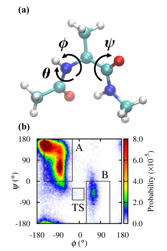
Figure 1: (a) Schematic representation of the alanine dipeptide molecule and its major dihedral angles, $\phi\left(\mathrm{C-N-C_{\alpha}-C}\right)$, $\psi\left(\mathrm{N-C_{\alpha}-C-N}\right)$, and $\theta\left(\mathrm{O-C-N-C_{\alpha}}\right)$. (b) Ramachandran plot of alanine dipeptide in vacuum. The regions described in boxes are defined as A: ($-150^{\circ}\leq\phi\leq-30^{\circ}$, $0^{\circ}\leq\psi\leq 180^{\circ}$), B: ($30^{\circ}\leq{\phi}\leq 130^{\circ}$, $-180^{\circ}\leq{\psi}\leq 0^{\circ}$), and TS: ($-30^{\circ}\leq{\phi}\leq 20^{\circ}$, $-80^{\circ}\leq{\psi}\leq-30^{\circ}$).

II.1 Likelihood maximization and cross-entropy minimization

We start from $N$ snapshots of the system that are sampled from the path connecting the reactant A and product B. We describe each snapshot $k$ by $M$ CVs $q_{i}(\mathbf{x}_{k})$, which are functions of the Cartesian coordinates $\mathbf{x}_{k}$. The committor calculated at each point from multiple short simulations is denoted as $p_{\mathrm{B}}^{*}\left(\mathbf{x}_{k}\right)$.

We aim at obtaining a RC that can describe the change of committor distribution $p_{\mathrm{B}}^{*}$ in a sigmoidal manner. To this end, we define the CV vector $\mathbf{q}(\mathbf{x}_{k})=(1,q_{1}(\mathbf{x}_{k}),\cdots,q_{M}(\mathbf{x}_{k}))$ and corresponding coefficients $\bm{\alpha}=(\alpha_{0},\alpha_{1},\cdots,\alpha_{M})$. Note that $\mathbf{q}$ is ($M$+1)-dimensional due to the bias term ($q_{0}=1$). We describe the trial function $r\left(\mathbf{q}\left(\mathbf{x}_{k}\right)\right)$ as a linear combination of the CVs as

$$r\left(\mathbf{q}\left(\mathbf{x}_{k}\right)\right)=\bm{\alpha}\cdot\mathbf{q}\left(\mathbf{x}_{k}\right)=\sum^{M}_{m=1}\alpha_{m}q_{m}\left(\mathbf{x}_{k}\right)+\alpha_{0}.$$ (1)

We assume that, in the ideal case, the committor $p_{\mathrm{B}}$ changes from 0 to 1 following the sigmoid function defined by

$$p_{\mathrm{B}}\left(r\left(\mathbf{q}\left(\mathbf{x}_{k}\right)\right)\right)=\frac{1+\tanh\left(r\left(\mathbf{q}\left(\mathbf{x}_{k}\right)\right)\right)}{2}.$$ (2)

Using Eq. (2), the Likelihood function $\mathcal{L}\left(\bm{\alpha}\right)$ can be defined as

$$\mathcal{L}\left(\bm{\alpha}\right)=\prod_{\mathbf{x}_{k}\rightarrow\mathrm{B}}p_{\mathrm{B}}\left(r\left(\mathbf{q}\left(\mathbf{x}_{k}\right)\right)\right)\times\prod_{\mathbf{x}_{k}\rightarrow\mathrm{A}}\left(1-p_{\mathrm{B}}\left(r\left(\mathbf{q}\left(\mathbf{x}_{k}\right)\right)\right)\right),$$ (3)

which was originally introduced by Peters et al. Peters, Beckham, and Trout (2007) Here, $\mathbf{x}_{k}\rightarrow\mathrm{B}$ and $\mathbf{x}_{k}\rightarrow\mathrm{A}$ indicate the trajectories starting from point $\mathbf{x}_{k}$ that ends in state B and A, respectively. By taking the logarithmic form of Eq. (3), we obtain

$$\ln{\mathcal{L}}\left(\bm{\alpha}\right)=\sum_{\mathbf{x}_{k}\rightarrow\mathrm{B}}\ln{p_{\mathrm{B}}\left(r\left(\mathbf{q}\left(\mathbf{x}_{k}\right)\right)\right)}+\sum_{\mathbf{x}_{k}\rightarrow\mathrm{A}}\ln{\left[1-p_{\mathrm{B}}\left(r\left(\mathbf{q}\left(\mathbf{x}_{k}\right)\right)\right)\right]}.$$ (4)

While each point $\mathbf{x}_{k}$ has a fractional probability to reach either state A or B, Eq. (4) can only account for each point in a binary manner to state A ($p_{\mathrm{B}}^{*}\left(\mathbf{x}_{k}\right)=0$) or B ($p_{\mathrm{B}}^{*}\left(\mathbf{x}_{k}\right)=1$). To make use of the continuous nature of the committor obtained directly, we extend Eq. (4) to

$$\mathcal{H}\left(p_{\mathrm{B}}^{*},p_{\mathrm{B}}\right)$$

$$\quad=-\sum_{k=1}^{N}p_{\mathrm{B}}^{*}\left(\mathbf{x}_{k}\right)\ln{p_{\mathrm{B}}\left(r\left(\mathbf{q}\left(\mathbf{x}_{k}\right)\right)\right)}$$

$$\quad\quad-\sum_{k=1}^{N}\left(1-p_{\mathrm{B}}^{*}\left(\mathbf{x}_{k}\right)\right)\ln{\left[1-p_{\mathrm{B}}\left(r\left(\mathbf{q}\left(\mathbf{x}_{k}\right)\right)\right)\right]},$$ (5)

which is equivalent to the cross-entropy. Note that Eq. (5) is derived from the Kullback–Leibler divergence in Ref. Mori and Saito, 2020. Equations (4) and (5) are equivalent with the opposite sign when $p_{\mathrm{B}}^{*}$ is binary:

$$p_{\mathrm{B}}^{*}=\left\{\begin{array}[]{ll}0&\left(\mathbf{x}_{k}\rightarrow\mathrm{A}\right)\\ 1&\left(\mathbf{x}_{k}\rightarrow\mathrm{B}\right)\end{array}\right.$$ (8)

Thus, the likelihood maximization is generalized to the cross-entropy minimization, considering the continuous nature of the committor. Note that $\mathcal{H}(p_{\mathrm{B}}^{*},p_{\mathrm{B}})\geq\mathcal{H}(p_{\mathrm{B}}^{*})\equiv\mathcal{H}(p_{\mathrm{B}}^{*},p_{\mathrm{B}}=p_{\mathrm{B}}^{*})$, where $\mathcal{H}(p_{\mathrm{B}}^{*})$ sets the lower bound of the cross-entropy.

II.2 $\bm{L_{2}}$-norm regularization

When the number of CVs used to describe the trial function $r\left(\mathbf{q}\left(\mathbf{x}_{k}\right)\right)$ is large, resulting reaction coordinate via the cross-entropy minimization can overfit the input data. To avoid overfitting, we introduced a technique called regularization that considers a penalty term in the objective function. In particular, we used the $L_{2}$-norm regularization. Bishop (2006) The objective function with the regularization is,

$$\mathcal{H}\left(\bm{\alpha}\right)=\mathcal{H}\left(p_{\mathrm{B}}^{*},p_{\mathrm{B}}\right)+\frac{\lambda}{2}\sum^{M}_{m=1}\alpha_{m}^{2},$$ (9)

where $\lambda$ is the regularization parameter that controls the relative weight of the penalty term. Note that the bias term $\alpha_{0}$ is not included in the regularization.

III Computational details

III.1 Sampling global conformational space

The isomerization of alanine dipeptide in vacuum was studied. One molecule of alanine dipeptide was placed in the 3.16 nm cubic box with the periodic boundary conditions. Time step of 1 fs, neighbor-list distance of 1.5 nm, van der Waals cut-off distance of 1.2 nm, switch function cut-off distance of 1.0 nm were used. For electrostatic interaction, the particle-mesh Ewald method was used with real-space cut-off distance of 1.2 nm. All covalent bonds were constrained by the LINCS algorithm. The AMBER99SB force field was used. Hornak et al. (2006) All simulations were conducted with GROMACS2018.1. Abraham et al. (2015)

The Ramachandran plot was generated from the replica-exchange MD (REMD) simulation. Sugita and Okamoto (1999) In the setup of MD simulations, 1 ns equilibration was followed by 10 ns production run with NVT condition at 300 K by using the Langevin thermostat. In the REMD simulations, 10 replicas were prepared in the range of 300 - 1209 K with 101 K interval. The exchange frequency was set to 200 fs, and the average exchange rate was 0.3.

III.2 Sampling conformations in transition state region

As mentioned in Sec. I, Peters et al., proposed a variant of transition path sampling called “aimless shooting.” Peters and Trout (2006) In this method, trajectories are generated with freshly sampled momenta from the Maxwell–Boltzmann distribution from every conformation.

In this study, we conducted the two-point version of the aimless shooting following the protocol in Ref. Peters, Beckham, and Trout, 2007. We initiated the aimless shooting from a conformation randomly chosen from the TS region (see below and Fig. 1(b) for the definition of the state). $\tau=2.01$ ps and $\delta{t}=10$ fs were used. Originally, the aimless shooting was introduced to sample conformations near $p_{\mathrm{B}}^{*}=1/2$. However, as mentioned in Sec. I, our purpose is to sample points that uniformly cover committor $p_{\mathrm{B}}^{*}$ values from 0 to 1. For this, we incorporated the shooing point even if the trajectory was rejected. We sampled 2,000 shooting points in total (accepted and rejected trajectories), which are divided equally into training and test datasets. From each point, we quantified $p_{\mathrm{B}}^{*}$ by running 1 ps MD simulations 100 times with random velocities from the Maxwell-Boltzmann distribution at 300 K.

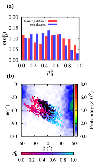
Figure 2: (a) Probability of committor value $p_{\mathrm{B}}^{*}$ for the training (red) and test (blue) datasets. Each dataset consists of 1,000 points, and $p_{\mathrm{B}}^{*}$ for each point is calculated from 100 trajectories. (b) Distribution of the training data points plotted on the Ramachandran plot of Fig. 1(b). The points are colored by the $p_{\mathrm{B}}^{*}$ values given in the bottom color bar. In addition, the points with $p_{\mathrm{B}}^{*}\sim 0.5$ ($0.45\leq p_{\mathrm{B}}^{*}\leq 0.55$) are marked in black dots.

III.3 Reaction coordinate optimization via cross-entropy minimization

Using the $p_{\mathrm{B}}^{*}$ values, we performed the cross-entropy minimization. We considered 45 dihedral angles (see Fig. S1 and Table S1 of Supplementary Material). These dihedral angles were transformed into cosine and sine forms, considering the periodicity. Thus, the dimension of $\bm{\alpha}$ is 91 ($M=90$ plus 1 bias term). The steepest descent method was used to update the coefficients $\bm{\alpha}$ as,

$$\bm{\alpha}^{(n+1)}=\bm{\alpha}^{(n)}-\gamma\nabla\mathcal{H}\left(\bm{\alpha}^{(n)}\right),$$ (10)

where $\bm{\alpha}^{(n)}$ and $\bm{\alpha}^{(n+1)}$ are the parameters at the $n$-th and ($n$+1)-th steps, respectively. $\nabla\mathcal{H}(\bm{\alpha}^{(n)})$ represents the gradient at the $n$-th step and $\gamma$ is the step size which was fixed to $10^{-5}$. The optimal $\bm{\alpha}$ was determined when the norm of $\nabla\mathcal{H}\left(\bm{\alpha}\right)$ becomes less than $\varepsilon=10^{-3}$. The regularization parameter was chosen as $\lambda=0$, 0.1, 0.5, 1, 10, and 100. To check the robustness of the optimization, we ran 10 optimization trials from the initial coefficients $\alpha_{i}$ that are randomly sampled from the range of $-0.1\leq\alpha_{i}\leq 0.1$.

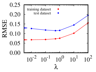
Figure 3: RMSEs of the training (red) and test (blue) datasets as a function of the regularization parameter $\lambda$. RMSE values of $\lambda=0$ are indicated by the arrows.

IV Results and discussion

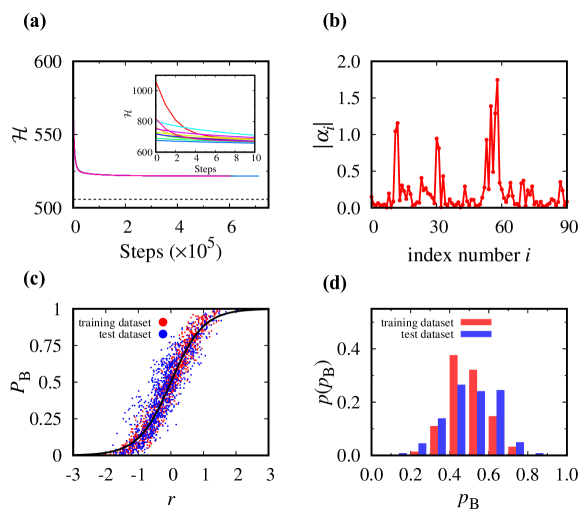
Figure 4: Summary of the parameter optimization for $\lambda=0.5$. (a) Changes of the cross-entropy function ($\mathcal{H}$) during the optimization steps (solid lines) and the ideal value $\mathcal{H}(p_{\mathrm{B}}^{*})$ (black dashed line). The results for the 10 trials using different initial $\bm{\alpha}$-guesses are shown in different colors. The inset focuses on the first 10 steps, showing that $\mathcal{H}$ differs remarkably in the beginning but quickly converges to a similar value within 10 steps. (b) Optimized coefficients ($\alpha_{i}$) in absolute value. Note that the coefficients are determined as an average over the 10 trials. (c) Committor distributions of the training (red) and test (blue) datasets as a function of the optimized coordinate $r$. The sigmoid function (Eq. (2)) is shown in black line. (d) Probability of $p_{\mathrm{B}}$ at about the TS of $r$ ($-0.2\leq r\leq 0.2$), where the points are extracted from the data shown in (c).

Table 1: First ten dominant coefficients after optimization using $\lambda=0.5$. The results are given as a mean and standard deviation of 10 trials starting from different initial conditions. The index follows the list given in Table S1 of Supplementary Material.

index	$\alpha_{i}$	standard deviation
$58$	$1.7453$	$2.2132\times 10^{-3}$
$55$	$1.3872$	$1.4342\times 10^{-3}$
$57$	$-1.2905$	$1.3520\times 10^{-3}$
$12$	$1.1562$	$1.2566\times 10^{-3}$
$11$	$-1.0431$	$1.4347\times 10^{-3}$
$30$	$-0.9451$	$1.2216\times 10^{-3}$
$53$	$-0.9275$	$1.2669\times 10^{-3}$
$31$	$0.8127$	$1.2908\times 10^{-3}$
$56$	$-0.4889$	$1.1470\times 10^{-3}$
$33$	$-0.4320$	$1.4202\times 10^{-3}$

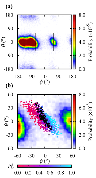
Figure 5: (a) Contour plot of the probability distribution as a function of $\phi$ and $\theta$. The probability distribution, calculated from the REMD trajectory, is described by a color bar on the right side of the plot. (b) Distribution of the training data points plotted on the probability distribution given in the squared region of (a). The points are colored by the $p_{\mathrm{B}}^{*}$ values given in the bottom color bar. In addition, the points with $p_{\mathrm{B}}^{*}\sim 0.5$ ($0.45\leq p_{\mathrm{B}}^{*}\leq 0.55$) are marked in black dots.

IV.1 Training and test datasets of committor values $\bm{p_{\mathrm{B}}^{*}}$

The Ramachandran plot obtained from the REMD trajectory is shown in Fig. 1(b). The two stable states, namely C7_eq and C7_ax, are found at $\phi\sim-90^{\circ}$ and $\phi\sim 60^{\circ}$, respectively. For simplicity, hereafter we denote the C7_eq and C7_ax states as A and B, respectively. Here we examine paths connecting states A and B, which possibly passes through TS region at $\psi\sim-50^{\circ}$ and $\phi\sim 0^{\circ}$. Note that these paths have also been of focus in the previous studies. Bolhuis, Dellago, and Chandler (2000); Ma and Dinner (2005); Ren et al. (2005) The snapshots along this path are sampled using the aimless shooting protocol as described in Sec. III.2. To optimize and validate the RC, we prepared two datasets, i.e., training and test, each consisting of 1,000 points. The committor value $p_{\mathrm{B}}^{*}$ for each point was calculated by running 100 short trajectories (see also Sec. III.2). Figure 2(a) shows the committor distribution for the training and test datasets. We see that the two datasets both fully cover $0\leq p_{\mathrm{B}}^{*}\leq 1$ with roughly similar probabilities. When the points are plotted on the Ramachandran plot (shown in Fig. 2(b)), we find that $\phi$ and $\psi$ can roughly separate points reaching state A ($p_{\mathrm{B}}<1/2$) and B ($p_{\mathrm{B}}>1/2$). Yet, the points with $p_{\mathrm{B}}^{*}\sim 0.5$ are spread out in the ($\phi$, $\psi$) space without a clear “separatrix” ($p_{\mathrm{B}}=1/2$ surface), indicating that the two coordinates are not sufficient in characterizing the TS. This unclear separatrix is in accord with a rather uniform distribution of the commmittor value $p_{\mathrm{B}}^{*}$ for the conformations of the TS on the $\phi$-$\psi$ plane that was demonstrated via the committor analysis in Ref. Bolhuis, Dellago, and Chandler, 2000.

IV.2 Minimizing cross-entropy and determining regularization parameter

We optimized the coefficients $\bm{\alpha}$ that minimize the cross-entropy function $\mathcal{H}(\bm{\alpha})$ (Eq. (9)) using the training dataset. To see the effect of the $L_{2}$-norm regularization, we changed the regularization parameter $\lambda$ in the range of 0 to 100, and performed the parameter optimization and validation. The performance against the training and test datasets were measured by the root-mean-squared-error (RMSE) between the expected (Eq. (2)) and raw committor values, defined as

$$\mathrm{RMSE}(\lambda)=\sqrt{\dfrac{1}{N}\sum_{k=1}^{N}\left[p_{B}^{\ast}(\mathbf{x}_{k})-p_{B}(r(\mathbf{q}(\mathbf{x}_{k})))\right]^{2}},$$ (11)

with $N=1000$ points. The results of RMSEs for different choices of $\lambda$ are summarized in Fig. 3. The figure shows that as $\lambda$ is increased, the RMSE of the training data gradually increase; on the contrary, the RMSE of the test data decreases until $\lambda\sim 1$, and starts to increase thereafter. Considering the balance between the performances of the training and test datasets, the optimal choice of $\lambda$ in the current case was determined to be $\lambda=0.5$. Below, we focus on the results obtained by fixing $\lambda$ to 0.5.

IV.3 Validation of the optimized parameter set

We examined the robustness of the optimization procedure using $\lambda=0.5$. Figure 4(a) shows that the cross-entropy function ($\mathcal{H}$) consistently converges to the same minimum when the initial guess for $\bm{\alpha}$ is varied. Figure 4(b) gives the optimized parameters (in absolute number), which is given as a mean of the 10 optimization trials. The result shows that several characteristic coordinates dominate the trial function $r(\mathbf{q}(\mathbf{x}_{k}))$; the raw coefficients of the major components are summarized in Table 1, and its full list is shown in Table S2 of Supplementary Material. For comparison, the results using $\lambda=0$ and $\lambda=10$ are also shown in Table S3 and Table S4 of Supplementary Material, respectively.

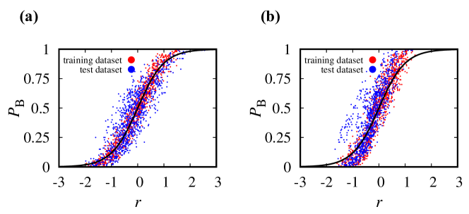
Figure S2: Committor distributions of the training (red) and test (blue) datasets as functions of the optimized coordinate $r$ for the cases of (a) $\lambda=0$ and (b) $\lambda=10$. The sigmoid function $p_{\mathrm{B}}(r)=[1+\tanh(r)]/2$ is shown in black line.

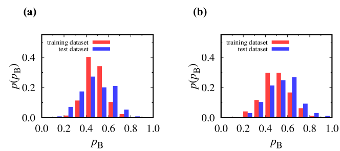
Figure S3: Probability of $p_{\mathrm{B}}$ at about the transition state of $r$ ($-0.2\leq r\leq 0.2$) for the cases of (a) $\lambda=0$ and (b) $\lambda=10$. Red and blue bars are for training and testing datasets, respectively.

Using the optimized coefficients, the performance of the predictability is tested using the test dataset. Figure 4(c) compares the distributions of the $p_{\mathrm{B}}$-value as a function of the optimized coordinate $r$. We see that overall the training and test datasets follow the sigmoid function (described as a black line in Fig. 4(c)), indicating that the optimized coordinate does serve as a good RC for the two datasets. We note that the test dataset tends to deviate slightly towards $p_{\mathrm{B}}$ value larger than the sigmoid function. Indeed, this trend can be confirmed by looking at the probability of $p_{\mathrm{B}}$ at about the TS of $r$ ($-0.2\leq r\leq 0.2$), which is given in Fig. 4(d). The probability show that while the distribution of $p_{B}$ is sharply peaked at about $p_{\mathrm{B}}\sim 0.5$ for the training dataset, the peak for the test dataset becomes broad and the center is shifted slightly towards $p_{\mathrm{B}}\sim 0.6$. Despite these small differences, the two probabilities can be characterized by a single peak centered at $p_{\mathrm{B}}\sim 0.5$ and with no points at $p_{\mathrm{B}}<0.1$ and $p_{\mathrm{B}}>0.9$. The current results thus confirm that the optimal RC determined using the training dataset is able to characterize the TS of the training dataset. Note that the results corresponding to Fig. 4(c) and Fig. 4(d) for $\lambda=0$ and $\lambda=10$ are shown in Fig. S2 and Fig. S3 of Supplementary Material, respectively.

IV.4 Character of the optimized reaction coordinate

As described in Fig. 4(b) and Table 1, the optimal coordinate can be characterized with a few dominant CVs. The first two components, $\alpha_{58}$, and $\alpha_{55}$, corresponds to the coefficient of $\sin{\phi}$ (5-7-9-15) and $\sin{\theta}$ (6-5-7-9), respectively (see also Fig. S1 and Table S1 of Supplementary Material). Note that these coordinates have been proposed to be important by Bolhuis et al. Bolhuis, Dellago, and Chandler (2000) The other major components, $\alpha_{57}$, $\alpha_{12}$, and $\alpha_{11}$, are also the rotations about the $\mathrm{C-N-C_{\alpha}}$ and $\mathrm{C-N}$ bonds (see Fig. 1(a)); $\psi$ only comes as a sixth component (as $\alpha_{30}$). The rotations about $\mathrm{C-N-C_{\alpha}}$ and $\mathrm{C-N}$ bonds, which can be characterized by $\phi$ and $\theta$, respectively, are thus suggested to be critical in characterizing the current TS of interest.

Finally, to confirm this insight, the committor distribution is examined on the probability distribution of $\phi$ and $\theta$, which was also obtained from the REMD trajectory and plotted in Fig. 5(a). Note that the two states A and B are found at $\phi\sim-90^{\circ}$ and $\phi\sim 60^{\circ}$, respectively, whereas the angle $\theta$ is mostly located at $\theta\sim 0^{\circ}$ regardless of the states. The training dataset points are described as a function of $\phi$ and $\theta$ in Fig. 5(b). We see that, in contrast to the $\phi$-$\psi$ plot in Fig. 2(b), the points with $p_{\mathrm{B}}^{*}\sim 0.5$ are narrowly distributed along a diagonal line in the $\phi$-$\theta$ plot (Fig. 5(b)), indicative of a clearer separatrix. This confirms that coupled changes of $\phi$ and $\theta$ are important for the TS along the path connecting states A and B. It is also consistent with the committor distributions showing the peak at $p_{\mathrm{B}}=1/2$ evaluated either by the transition state sampling Bolhuis, Dellago, and Chandler (2000) or by the umbrella sampling Ma and Dinner (2005) on the $\phi$-$\theta$ plane. In conclusion, it is demonstrated the method of the minimization of the cross-entropy function $\mathcal{H}$ combined with the $L_{2}$-norm regularization can guide the straightforward way to find the RC that appropriately describes the TS.

V Conclusions

In this paper, we proposed a cross-entropy minimization method to identify the RC from a large number of CVs using the committor dataset $p_{\mathrm{B}}^{*}$. The method is a generalization of the likelihood maximization approach proposed by Peters et al., Peters, Beckham, and Trout (2007) and is also derived from the Kullback–Leibler divergence. Mori and Saito (2020) To take account of a large number of CVs and yet avoid overfitting, we further introduced the $L_{2}$-norm regularization technique. Bishop (2006)

Using the training and test datasets of committor $p_{\mathrm{B}}^{*}$, which are described as a function of the dihedral angles (in the cosine and sine forms), we minimized the cross-entropy function $\mathcal{H}$ and determined the optimal balance of the regularization penalty. We identified the appropriate RC capable of describing the TS of the isomerization reaction of alanine dipeptide in vacuum. The minimization of $\mathcal{H}$ was found to be quite stable, i.e., the parameters consistently converged to the same set independent of the initial guesses of $\bm{\alpha}$. The committor distribution at the TS ($r\sim 0$) was found to be peaked at $p_{\mathrm{B}}\sim 0.5$, both in the cases of the training and data sets. This result indicates that $r=0$ indeed describes the TS. The optimized coordinate was dominantly characterized by the dihedral angles $\phi$ and $\theta$. These CVs were further justified by the clear separatrix on the scattering plot on the $(\phi,\theta)$ plane. The presented result is consistent with the observation in the previous studies Bolhuis, Dellago, and Chandler (2000); Ma and Dinner (2005); Ren et al. (2005), which showed the importance of $\theta$ in characterizing the TS of this reaction.

Finally, it should be emphasized that selecting the appropriate RC becomes often cumbersome when considered CVs are possibly redundant and are also correlated with each other. Peters (2017) The current approach via the cross-entropy function combined with the $L_{2}$-norm regularization can be a powerful means to identify and characterize the RC from the $p_{\mathrm{B}}^{*}$ dataset.

Supplementary material

See supplementary material for dihedral angles and CV indices (Fig. S1 and Table S1), full list of optimal coordinate for $\lambda=0$, 0.5, and 10 (Table S2, Table S3, and Table S4, respectively), committor distributions as a function of the optimized coordinate for $\lambda=0$ and 10 (Fig. S2), and $p_{\mathrm{B}}$ probability at about the TS of $r$ ($-0.2\leq r\leq 0.2$) for $\lambda=0$ and 10 (Fig. S3).

Data availability statement

The data supporting the findings of this study are available from the corresponding authors upon reasonable request.

Supplementary Material

Learning reaction coordinates via cross-entropy minimization:
Application to alanine dipeptide

Yusuke Mori¹, Kei-ichi Okazaki², Toshifumi Mori^2,3, Kang Kim^1,2, Nobuyuki Matubayasi¹

¹Division of Chemical Engineering, Graduate School of Engineering Science, Osaka University, Osaka 560-8531, Japan
²Institute for Molecular Science, Okazaki, Aichi 444-8585, Japan
³The Graduate University for Advanced Studies, Okazaki, Aichi 444-8585, Japan

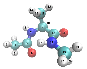
Figure S1: Schematic representation of the alanine dipeptide molecule and the numbering of atoms.

Table S1: Definition of the dihedral angle coordinates corresponding to the coefficients $\alpha_{i}$. The atom numbers are defined in Fig. S1. Note that the dihedral angles are used in cosine and sine forms, i.e., $\alpha_{01}$ to $\alpha_{45}$ and $\alpha_{46}$ to $\alpha_{90}$ are the cosine and sine forms, respectively.

index	atom number
$01-03$	2 - 1 - 5 - 6	2 - 1 - 5 - 7	3 - 1 - 5 - 6
$04-06$	3 - 1 - 5 - 7	4 - 1 - 5 - 6	4 - 1 - 5 - 7
$07-09$	1 - 5 - 7 - 8	1 - 5 - 7 - 9	6 - 5 - 7 - 8
$10-12$	6 - 5 - 7 - 9	5 - 7 - 9 - 10	5 - 7 - 9 - 11
$13-15$	5 - 7 - 9 - 15	8 - 7 - 9 - 10	8 - 7 - 9 - 11
$16-18$	8 - 7 - 9 - 15	7 - 9 - 11 - 12	7 - 9 - 11 - 13
$19-21$	7 - 9 - 11 - 14	10 - 9 - 11 - 12	10 - 9 - 11 - 13
$22-24$	10 - 9 - 11 - 14	15 - 9 - 11 - 12	15 - 9 - 11 - 13
$25-27$	15 - 9 - 11 - 14	7 - 9 - 15 - 16	7 - 9 - 15 - 17
$28-30$	10 - 9 - 15 - 16	10 - 9 - 15 - 17	11 - 9 - 15 - 16
$31-33$	11 - 9 - 15 - 17	9 - 15 - 17 - 18	9 - 15 - 17 - 19
$34-36$	16 - 15 - 17 - 18	16 - 15 - 17 - 19	15 - 17 - 19 - 20
$37-39$	15 - 17 - 19 - 21	15 - 17 - 19 - 22	18 - 17 - 19 - 20
$40-42$	18 - 17 - 19 - 21	18 - 17 - 19 - 22	1 - 7 - 5 - 6
$43-45$	5 - 9 - 7 - 8	9 - 17 - 15 - 16	15 - 19 - 17 - 18

Table S2: Full list of optimized coefficients for $\lambda=0.5$ in descending order. The coefficients are calculated as a mean over 10 optimization trials with different initial parameters, and the standard deviations are also calculated from that data.

index	$\alpha_{i}$	standard deviation	index	$\alpha_{i}$	standard deviation
$58$	$1.7453$	$2.2132\times 10^{-3}$	$44$	$0.0893$	$3.7040\times 10^{-3}$
$55$	$1.3872$	$1.4342\times 10^{-3}$	$10$	$-0.0852$	$5.4605\times 10^{-4}$
$57$	$-1.2905$	$1.3520\times 10^{-3}$	$78$	$0.0831$	$1.8153\times 10^{-3}$
$12$	$1.1562$	$1.2566\times 10^{-3}$	$90$	$0.0822$	$4.9167\times 10^{-5}$
$11$	$-1.0431$	$1.4347\times 10^{-3}$	$76$	$-0.0797$	$1.5140\times 10^{-3}$
$30$	$-0.9451$	$1.2216\times 10^{-3}$	$62$	$-0.0794$	$1.2742\times 10^{-3}$
$53$	$-0.9275$	$1.2669\times 10^{-3}$	$86$	$0.0783$	$4.0652\times 10^{-4}$
$31$	$0.8127$	$1.2908\times 10^{-3}$	$21$	$0.0752$	$1.6528\times 10^{-3}$
$56$	$-0.4889$	$1.1470\times 10^{-3}$	$40$	$0.0751$	$6.5192\times 10^{-4}$
$33$	$-0.4320$	$1.4202\times 10^{-3}$	$22$	$-0.0693$	$1.4945\times 10^{-3}$
$23$	$-0.4079$	$1.4942\times 10^{-3}$	$03$	$0.0633$	$1.2441\times 10^{-3}$
$70$	$0.3702$	$1.8008\times 10^{-3}$	$37$	$0.0629$	$3.7637\times 10^{-4}$
$87$	$-0.3522$	$1.1409\times 10^{-3}$	$29$	$-0.0610$	$1.1698\times 10^{-3}$
$64$	$0.3417$	$2.4532\times 10^{-3}$	$82$	$-0.0600$	$7.0894\times 10^{-4}$
$59$	$-0.3412$	$5.7088\times 10^{-4}$	$67$	$0.0529$	$1.4246\times 10^{-3}$
$69$	$-0.3336$	$1.4729\times 10^{-3}$	$34$	$0.0525$	$9.6742\times 10^{-4}$
$14$	$-0.3058$	$4.7081\times 10^{-4}$	$66$	$0.0484$	$1.6093\times 10^{-3}$
$74$	$-0.2931$	$1.4450\times 10^{-3}$	$01$	$-0.0474$	$1.2315\times 10^{-3}$
$43$	$-0.2916$	$3.6195\times 10^{-4}$	$50$	$0.0474$	$1.3886\times 10^{-3}$
$17$	$-0.2855$	$2.0916\times 10^{-3}$	$75$	$-0.0458$	$1.9937\times 10^{-3}$
$52$	$-0.2774$	$1.8192\times 10^{-3}$	$06$	$0.0448$	$1.1690\times 10^{-3}$
$25$	$0.2683$	$1.7937\times 10^{-3}$	$20$	$-0.0446$	$1.0052\times 10^{-3}$
$54$	$-0.2524$	$1.8326\times 10^{-3}$	$42$	$-0.0419$	$2.8231\times 10^{-3}$
$60$	$-0.2518$	$1.3573\times 10^{-3}$	$39$	$-0.0419$	$3.9380\times 10^{-4}$
$24$	$0.2390$	$1.5487\times 10^{-3}$	$81$	$0.0413$	$8.6112\times 10^{-4}$
$72$	$0.2374$	$2.9760\times 10^{-3}$	$05$	$-0.0380$	$1.1829\times 10^{-3}$
$88$	$-0.2369$	$1.5089\times 10^{-3}$	$04$	$-0.0343$	$1.2638\times 10^{-3}$
$15$	$-0.2283$	$1.1347\times 10^{-3}$	$89$	$-0.0342$	$1.5882\times 10^{-3}$
$26$	$-0.1978$	$2.2601\times 10^{-3}$	$02$	$-0.0336$	$1.2283\times 10^{-3}$
$08$	$0.1955$	$1.1138\times 10^{-3}$	$45$	$-0.0329$	$1.5147\times 10^{-4}$
$18$	$0.1869$	$1.4237\times 10^{-3}$	$85$	$0.0328$	$4.5792\times 10^{-4}$
$27$	$0.1803$	$2.5249\times 10^{-3}$	$38$	$0.0318$	$6.1766\times 10^{-4}$
$73$	$0.1789$	$1.5840\times 10^{-3}$	$35$	$0.0302$	$2.1288\times 10^{-3}$
$63$	$-0.1638$	$1.4197\times 10^{-3}$	$49$	$-0.0281$	$1.2168\times 10^{-3}$
$65$	$-0.1600$	$1.5497\times 10^{-3}$	$71$	$0.0266$	$1.6182\times 10^{-3}$
$00$	$-0.1501$	$1.7866\times 10^{-2}$	$48$	$-0.0265$	$1.2725\times 10^{-3}$
$28$	$0.1406$	$1.8230\times 10^{-3}$	$19$	$-0.0254$	$1.2048\times 10^{-3}$
$51$	$0.1394$	$1.4095\times 10^{-3}$	$79$	$0.0222$	$1.7288\times 10^{-3}$
$61$	$-0.1337$	$1.5507\times 10^{-3}$	$77$	$-0.0218$	$1.6835\times 10^{-3}$
$16$	$0.1215$	$3.9594\times 10^{-4}$	$80$	$-0.0165$	$1.8729\times 10^{-3}$
$83$	$0.1181$	$3.5624\times 10^{-4}$	$68$	$0.0147$	$1.3306\times 10^{-3}$
$36$	$0.1160$	$6.7586\times 10^{-4}$	$32$	$0.0083$	$1.1014\times 10^{-3}$
$46$	$0.1109$	$8.6875\times 10^{-4}$	$09$	$0.0060$	$2.2018\times 10^{-4}$
$47$	$-0.1089$	$8.5633\times 10^{-4}$	$41$	$-0.0049$	$5.2831\times 10^{-4}$
$13$	$-0.1017$	$1.3712\times 10^{-3}$	$07$	$-0.0049$	$2.2382\times 10^{-4}$
$84$	$0.1005$	$1.0053\times 10^{-3}$

Table S3: Full list of optimized coefficients for $\lambda=0$ in descending order. The coefficients are calculated as a mean over 10 optimization trials with different initial parameters, and the standard deviations are also calculated from that data.

index	$\alpha_{i}$	standard deviation	index	$\alpha_{i}$	standard deviation
$58$	$3.1511$	$5.1786\times 10^{-3}$	$61$	$0.4045$	$2.5976\times 10^{-3}$
$55$	$2.6830$	$1.4032\times 10^{-2}$	$78$	$-0.4023$	$3.4432\times 10^{-2}$
$33$	$-2.5446$	$4.1285\times 10^{-3}$	$83$	$0.3947$	$4.6369\times 10^{-4}$
$57$	$-2.4873$	$2.1762\times 10^{-3}$	$01$	$0.3868$	$7.7135\times 10^{-3}$
$00$	$-2.4527$	$1.1267\times 10^{-2}$	$63$	$-0.3619$	$3.0409\times 10^{-2}$
$31$	$2.1781$	$2.3398\times 10^{-2}$	$19$	$-0.3565$	$1.4991\times 10^{-2}$
$72$	$1.9539$	$2.0216\times 10^{-2}$	$21$	$-0.3389$	$3.2438\times 10^{-2}$
$88$	$-1.9151$	$6.4681\times 10^{-4}$	$73$	$-0.3162$	$3.2698\times 10^{-2}$
$30$	$-1.5587$	$2.4409\times 10^{-2}$	$02$	$0.3098$	$7.6417\times 10^{-3}$
$51$	$1.4762$	$1.0109\times 10^{-2}$	$22$	$0.3030$	$2.7601\times 10^{-2}$
$50$	$1.3540$	$1.0037\times 10^{-2}$	$66$	$0.2748$	$1.8121\times 10^{-2}$
$11$	$-1.2952$	$5.0231\times 10^{-3}$	$56$	$-0.2683$	$2.3946\times 10^{-3}$
$87$	$1.2813$	$1.2720\times 10^{-2}$	$25$	$0.2247$	$1.5989\times 10^{-2}$
$23$	$-1.2131$	$2.6910\times 10^{-2}$	$17$	$-0.2183$	$3.6273\times 10^{-2}$
$74$	$-1.1767$	$3.2587\times 10^{-2}$	$38$	$-0.2111$	$6.6435\times 10^{-4}$
$64$	$1.1428$	$2.3731\times 10^{-2}$	$85$	$0.1958$	$4.1448\times 10^{-4}$
$60$	$-1.1346$	$5.5465\times 10^{-4}$	$40$	$0.1867$	$6.7666\times 10^{-4}$
$13$	$-1.0363$	$2.4769\times 10^{-3}$	$53$	$0.1794$	$1.3984\times 10^{-2}$
$35$	$-1.0152$	$5.7957\times 10^{-3}$	$29$	$-0.1559$	$6.2233\times 10^{-3}$
$26$	$-1.0069$	$3.1832\times 10^{-2}$	$39$	$0.1538$	$4.4290\times 10^{-4}$
$67$	$0.9278$	$1.7525\times 10^{-2}$	$42$	$-0.1359$	$7.2953\times 10^{-3}$
$54$	$-0.9158$	$2.3805\times 10^{-3}$	$20$	$0.1330$	$9.2173\times 10^{-4}$
$52$	$-0.9051$	$2.3491\times 10^{-3}$	$41$	$-0.1272$	$6.2702\times 10^{-4}$
$71$	$0.8552$	$1.9949\times 10^{-2}$	$82$	$0.1268$	$6.4682\times 10^{-4}$
$12$	$0.8358$	$2.3220\times 10^{-3}$	$28$	$-0.1038$	$6.6050\times 10^{-3}$
$46$	$0.7259$	$9.4158\times 10^{-3}$	$07$	$0.1030$	$6.6437\times 10^{-4}$
$65$	$-0.6920$	$2.6471\times 10^{-2}$	$75$	$-0.0929$	$1.7938\times 10^{-2}$
$70$	$0.6651$	$3.4239\times 10^{-2}$	$69$	$0.0900$	$2.3117\times 10^{-2}$
$15$	$0.6425$	$1.1172\times 10^{-3}$	$08$	$-0.0854$	$1.9408\times 10^{-3}$
$47$	$0.5937$	$9.4431\times 10^{-3}$	$36$	$0.0847$	$3.3590\times 10^{-4}$
$80$	$-0.5795$	$3.4149\times 10^{-2}$	$90$	$0.0836$	$4.5581\times 10^{-5}$
$49$	$0.5640$	$6.9340\times 10^{-3}$	$43$	$-0.0797$	$2.6093\times 10^{-4}$
$84$	$0.5562$	$7.6356\times 10^{-4}$	$14$	$-0.0766$	$1.3332\times 10^{-3}$
$10$	$-0.5522$	$2.8041\times 10^{-3}$	$68$	$-0.0761$	$1.4963\times 10^{-2}$
$76$	$0.5451$	$1.8858\times 10^{-2}$	$32$	$-0.0745$	$2.0748\times 10^{-3}$
$62$	$0.5373$	$1.3239\times 10^{-2}$	$09$	$0.0496$	$6.3746\times 10^{-4}$
$48$	$0.5277$	$7.1636\times 10^{-3}$	$37$	$0.0462$	$3.7478\times 10^{-4}$
$81$	$0.5218$	$6.9539\times 10^{-4}$	$77$	$-0.0438$	$3.0750\times 10^{-3}$
$24$	$0.5206$	$2.0542\times 10^{-2}$	$79$	$0.0288$	$3.1391\times 10^{-3}$
$27$	$0.5132$	$3.3043\times 10^{-2}$	$34$	$-0.0206$	$1.9660\times 10^{-3}$
$04$	$-0.4836$	$1.1262\times 10^{-2}$	$05$	$0.0176$	$9.6553\times 10^{-3}$
$44$	$0.4811$	$3.2205\times 10^{-3}$	$89$	$0.0165$	$3.1549\times 10^{-2}$
$18$	$0.4788$	$1.1043\times 10^{-2}$	$16$	$-0.0136$	$6.3249\times 10^{-4}$
$59$	$-0.4441$	$1.2642\times 10^{-3}$	$06$	$0.0112$	$9.4690\times 10^{-3}$
$86$	$0.4393$	$6.8539\times 10^{-4}$	$45$	$-0.0090$	$1.3192\times 10^{-4}$
$03$	$-0.4289$	$1.1060\times 10^{-2}$

Table S4: Full list of optimized coefficients for $\lambda=10$ in descending order. The coefficients are calculated as a mean over 10 optimization trials with different initial parameters, and the standard deviations are also calculated from that data.

index	$\alpha_{i}$	standard deviation	index	$\alpha_{i}$	standard deviation
$58$	$0.8306$	$3.5528\times 10^{-11}$	$81$	$-0.0426$	$1.2914\times 10^{-10}$
$57$	$-0.6144$	$2.7921\times 10^{-9}$	$01$	$-0.0422$	$6.8381\times 10^{-11}$
$12$	$0.6061$	$2.3452\times 10^{-9}$	$04$	$-0.0379$	$3.6555\times 10^{-10}$
$55$	$0.5980$	$6.3127\times 10^{-10}$	$45$	$-0.0372$	$2.2530\times 10^{-9}$
$11$	$-0.5796$	$1.5295\times 10^{-9}$	$18$	$0.0372$	$3.6965\times 10^{-9}$
$53$	$-0.3841$	$3.6147\times 10^{-10}$	$68$	$0.0352$	$3.5254\times 10^{-9}$
$88$	$0.3787$	$1.0132\times 10^{-10}$	$65$	$-0.0350$	$1.5159\times 10^{-10}$
$30$	$-0.2475$	$1.5217\times 10^{-9}$	$50$	$0.0349$	$1.7245\times 10^{-10}$
$56$	$-0.2391$	$3.0540\times 10^{-9}$	$09$	$0.0317$	$1.2569\times 10^{-9}$
$61$	$-0.2257$	$3.9281\times 10^{-10}$	$51$	$0.0316$	$1.4641\times 10^{-10}$
$87$	$-0.2200$	$3.5622\times 10^{-10}$	$20$	$0.0313$	$3.2898\times 10^{-9}$
$15$	$-0.2189$	$3.5264\times 10^{-10}$	$84$	$0.0293$	$1.8027\times 10^{-10}$
$31$	$0.2153$	$1.7952\times 10^{-9}$	$34$	$0.0292$	$1.8532\times 10^{-9}$
$00$	$0.2084$	$1.0023\times 10^{-7}$	$64$	$0.0280$	$3.1097\times 10^{-9}$
$26$	$0.1699$	$2.0812\times 10^{-9}$	$41$	$-0.0280$	$6.1336\times 10^{-11}$
$27$	$-0.1531$	$1.8384\times 10^{-9}$	$83$	$0.0267$	$2.9348\times 10^{-10}$
$52$	$-0.1359$	$8.2253\times 10^{-11}$	$02$	$-0.0258$	$7.9951\times 10^{-11}$
$43$	$-0.1239$	$9.3277\times 10^{-10}$	$80$	$-0.0249$	$9.6400\times 10^{-10}$
$76$	$-0.1054$	$3.8599\times 10^{-9}$	$66$	$0.0240$	$2.8176\times 10^{-9}$
$75$	$0.0983$	$3.9213\times 10^{-9}$	$40$	$0.0238$	$1.2308\times 10^{-10}$
$13$	$0.0930$	$3.2933\times 10^{-9}$	$05$	$-0.0232$	$2.7483\times 10^{-10}$
$71$	$0.0898$	$3.4497\times 10^{-9}$	$89$	$-0.0231$	$3.0971\times 10^{-10}$
$60$	$0.0847$	$5.6629\times 10^{-10}$	$33$	$-0.0227$	$4.5047\times 10^{-9}$
$37$	$0.0800$	$2.0658\times 10^{-10}$	$10$	$-0.0213$	$3.0889\times 10^{-9}$
$25$	$0.0775$	$3.7010\times 10^{-9}$	$17$	$-0.0197$	$1.4371\times 10^{-9}$
$54$	$-0.0764$	$1.8622\times 10^{-10}$	$22$	$-0.0177$	$1.9466\times 10^{-9}$
$70$	$0.0752$	$8.2912\times 10^{-10}$	$85$	$-0.0147$	$2.2215\times 10^{-10}$
$69$	$-0.0711$	$2.7979\times 10^{-9}$	$74$	$0.0146$	$4.9195\times 10^{-11}$
$19$	$-0.0684$	$2.2126\times 10^{-9}$	$24$	$0.0146$	$2.4496\times 10^{-9}$
$23$	$-0.0677$	$1.2557\times 10^{-9}$	$08$	$-0.0137$	$3.4721\times 10^{-9}$
$03$	$0.0676$	$2.7891\times 10^{-10}$	$63$	$0.0136$	$4.5148\times 10^{-10}$
$39$	$-0.0646$	$1.6649\times 10^{-10}$	$21$	$0.0129$	$1.4208\times 10^{-9}$
$07$	$-0.0615$	$1.2193\times 10^{-9}$	$79$	$-0.0117$	$7.3789\times 10^{-10}$
$49$	$-0.0595$	$2.4875\times 10^{-10}$	$29$	$0.0086$	$4.0031\times 10^{-9}$
$72$	$-0.0594$	$3.5546\times 10^{-9}$	$32$	$0.0083$	$1.9369\times 10^{-9}$
$06$	$0.0588$	$3.5111\times 10^{-11}$	$48$	$-0.0078$	$2.5259\times 10^{-11}$
$82$	$-0.0554$	$5.5851\times 10^{-10}$	$14$	$0.0066$	$3.6773\times 10^{-10}$
$78$	$0.0527$	$6.9169\times 10^{-10}$	$42$	$-0.0064$	$4.6971\times 10^{-9}$
$90$	$0.0504$	$8.0539\times 10^{-10}$	$77$	$0.0059$	$1.0523\times 10^{-9}$
$86$	$0.0495$	$3.2697\times 10^{-11}$	$36$	$0.0057$	$2.3601\times 10^{-10}$
$62$	$-0.0472$	$3.4940\times 10^{-9}$	$35$	$0.0035$	$4.2877\times 10^{-9}$
$16$	$0.0455$	$8.4477\times 10^{-10}$	$28$	$-0.0035$	$3.9852\times 10^{-9}$
$46$	$0.0442$	$1.4667\times 10^{-11}$	$59$	$-0.0026$	$7.3267\times 10^{-10}$
$47$	$-0.0432$	$1.8039\times 10^{-10}$	$38$	$0.0022$	$4.3125\times 10^{-10}$
$73$	$-0.0431$	$3.1798\times 10^{-10}$	$44$	$-0.0017$	$4.6810\times 10^{-9}$
$67$	$-0.0430$	$2.7864\times 10^{-9}$

References

• Chipot and Pohorille (2007) C. Chipot and A. Pohorille, Free Energy Calculations: Theory and Applications in Chemistry and Biology (Springer, New York, 2007).
• Zuckerman (2010) D. M. Zuckerman, Statistical Physics of Biomolecules: An Introduction  (CRC Press, Boca Raton, 2010).
• Torrie and Valleau (1977) G. M. Torrie and J. P. Valleau, “Nonphysical sampling distributions in Monte Carlo free-energy estimation: Umbrella sampling,” J. Comput. Phys. 23, 187–199 (1977).
• Sugita and Okamoto (1999) Y. Sugita and Y. Okamoto, “Replica-exchange molecular dynamics method for protein folding,” Chem. Phys. Lett. 314, 141–151 (1999).
• Laio and Parrinello (2002) A. Laio and M. Parrinello, “Escaping free-energy minima,” Proc. Natl. Acad. Sci. U.S.A. 99, 12562–12566 (2002).
• Peters (2017) B. Peters, Reaction Rate Theory and Rare Events (Elsevier, Amsterdam, 2017).
• Bolhuis et al. (2002) P. G. Bolhuis, D. Chandler, C. Dellago,  and P. L. Geissler, “Transition path sampling: throwing ropes over rough mountain passes, in the dark.” Annu. Rev. Phys. Chem. 53, 291–318 (2002).
• Du et al. (1998) R. Du, V. S. Pande, A. Y. Grosberg, T. Tanaka,  and E. S. Shakhnovich, “On the transition coordinate for protein folding,” J. Chem. Phys. 108, 334–350 (1998).
• Geissler, Dellago, and Chandler (1999) P. L. Geissler, C. Dellago,  and D. Chandler, “Kinetic Pathways of Ion Pair Dissociation in Water,” J. Phys. Chem. B 103, 3706–3710 (1999).
• Bolhuis, Dellago, and Chandler (2000) P. G. Bolhuis, C. Dellago,  and D. Chandler, “Reaction coordinates of biomolecular isomerization,” Proc. Natl. Acad. Sci. U.S.A. 97, 5877–5882 (2000).
• Dellago, Bolhuis, and Geissler (2002) C. Dellago, P. G. Bolhuis,  and P. L. Geissler, “Transition Path Sampling,” in Adv. Chem. Phys., Vol. 123 (John Wiley & Sons, Ltd, 2002) pp. 1–78.
• Hagan et al. (2003) M. F. Hagan, A. R. Dinner, D. Chandler,  and A. K. Chakraborty, “Atomistic understanding of kinetic pathways for single base-pair binding and unbinding in DNA,” Proc. Natl. Acad. Sci. U.S.A. 100, 13922–13927 (2003).
• Hummer (2004) G. Hummer, “From transition paths to transition states and rate coefficients,” J. Chem. Phys. 120, 516–523 (2004).
• Pan and Chandler (2004) A. C. Pan and D. Chandler, “Dynamics of Nucleation in the Ising Model,” J. Phys. Chem. B 108, 19681–19686 (2004).
• Ma and Dinner (2005) A. Ma and A. R. Dinner, “Automatic Method for Identifying Reaction Coordinates in Complex Systems,” J. Phys. Chem. B 109, 6769–6779 (2005).
• Ren et al. (2005) W. Ren, E. Vanden-Eijnden, P. Maragakis,  and W. E, “Transition pathways in complex systems: Application of the finite-temperature string method to the alanine dipeptide,” J. Chem. Phys. 123, 134109 (2005).
• Rhee and Pande (2005) Y. M. Rhee and V. S. Pande, “One-Dimensional Reaction Coordinate and the Corresponding Potential of Mean Force from Commitment Probability Distribution,” J. Phys. Chem. B 109, 6780–6786 (2005).
• E, Ren, and Vanden-Eijnden (2005) W. E, W. Ren,  and E. Vanden-Eijnden, “Transition pathways in complex systems: Reaction coordinates, isocommittor surfaces, and transition tubes,” Chem. Phys. Lett. 413, 242–247 (2005).
• Berezhkovskii and Szabo (2005) A. Berezhkovskii and A. Szabo, “One-dimensional reaction coordinates for diffusive activated rate processes in many dimensions,” J. Chem. Phys. 122, 014503 (2005).
• Best and Hummer (2005) R. B. Best and G. Hummer, “Reaction coordinates and rates from transition paths,” Proc. Natl. Acad. Sci. U.S.A. 102, 6732–6737 (2005).
• Moroni, ten Wolde, and Bolhuis (2005) D. Moroni, P. R. ten Wolde,  and P. G. Bolhuis, “Interplay between Structure and Size in a Critical Crystal Nucleus,” Phys. Rev. Lett. 94, 235703 (2005).
• Peters (2006) B. Peters, “Using the histogram test to quantify reaction coordinate error,” J. Chem. Phys. 125, 241101 (2006).
• Branduardi, Gervasio, and Parrinello (2007) D. Branduardi, F. L. Gervasio,  and M. Parrinello, “From A to B in free energy space,” J. Chem. Phys. 126, 054103 (2007).
• Quaytman and Schwartz (2007) S. L. Quaytman and S. D. Schwartz, “Reaction coordinate of an enzymatic reaction revealed by transition path sampling,” Proc. Natl. Acad. Sci. U.S.A. 104, 12253–12258 (2007).
• Antoniou and Schwartz (2009) D. Antoniou and S. D. Schwartz, “The stochastic separatrix and the reaction coordinate for complex systems,” J. Chem. Phys. 130, 151103 (2009).
• Peters (2010a) B. Peters, “p(TP|q) peak maximization: Necessary but not sufficient for reaction coordinate accuracy,” Chem. Phys. Lett. 494, 100–103 (2010a).
• Peters (2010b) B. Peters, “Recent advances in transition path sampling: accurate reaction coordinates, likelihood maximisation and diffusive barrier-crossing dynamics,” Mol. Simul. 36, 1265–1281 (2010b).
• Li and Ma (2014) W. Li and A. Ma, “Recent developments in methods for identifying reaction coordinates.” Mol. Simul. 40, 784–793 (2014).
• Wales (2015) D. J. Wales, “Perspective: Insight into reaction coordinates and dynamics from the potential energy landscape,” J. Chem. Phys. 142, 130901 (2015).
• Peters (2016) B. Peters, “Reaction Coordinates and Mechanistic Hypothesis Tests,” Annu. Rev. Phys. Chem. 67, 669–690 (2016).
• Banushkina and Krivov (2016) P. V. Banushkina and S. V. Krivov, “Optimal reaction coordinates,” WIREs Comput Mol Sci 6, 748–763 (2016).
• Sittel and Stock (2018) F. Sittel and G. Stock, “Perspective: Identification of collective variables and metastable states of protein dynamics,” J. Chem. Phys. 149, 150901 (2018).
• Sultan and Pande (2018) M. M. Sultan and V. S. Pande, “Automated design of collective variables using supervised machine learning,” J. Chem. Phys. 149, 094106 (2018).
• Jung, Covino, and Hummer (2019) H. Jung, R. Covino,  and G. Hummer, “Artificial Intelligence Assists Discovery of Reaction Coordinates and Mechanisms from Molecular Dynamics Simulations,” arXiv  (2019), 1901.04595v1 .
• Noé et al. (2020) F. Noé, A. Tkatchenko, K.-R. Müller,  and C. Clementi, “Machine Learning for Molecular Simulation,” Annu. Rev. Phys. Chem. 71, 361–390 (2020).
• Sidky, Chen, and Ferguson (2020) H. Sidky, W. Chen,  and A. L. Ferguson, “Machine learning for collective variable discovery and enhanced sampling in biomolecular simulation,” Mol. Phys. 118, e1737742 (2020).
• Peters, Beckham, and Trout (2007) B. Peters, G. T. Beckham,  and B. L. Trout, “Extensions to the likelihood maximization approach for finding reaction coordinates,” J. Chem. Phys. 127, 034109 (2007).
• Peters and Trout (2006) B. Peters and B. L. Trout, “Obtaining reaction coordinates by likelihood maximization,” J. Chem. Phys. 125, 054108 (2006).
• Beckham et al. (2007) G. T. Beckham, B. Peters, C. Starbuck, N. Variankaval,  and B. L. Trout, “Surface-Mediated Nucleation in the Solid-State Polymorph Transformation of Terephthalic Acid,” J. Am. Chem. Soc. 129, 4714–4723 (2007).
• Beckham, Peters, and Trout (2008) G. T. Beckham, B. Peters,  and B. L. Trout, “Evidence for a Size Dependent Nucleation Mechanism in Solid State Polymorph Transformations,” J. Phys. Chem. B 112, 7460–7466 (2008).
• Vreede, Juraszek, and Bolhuis (2010) J. Vreede, J. Juraszek,  and P. G. Bolhuis, “Predicting the reaction coordinates of millisecond light-induced conformational changes in photoactive yellow protein,” Proc. Natl. Acad. Sci. U.S.A. 107, 2397–2402 (2010).
• Lechner et al. (2010) W. Lechner, J. Rogal, J. Juraszek, B. Ensing,  and P. G. Bolhuis, “Nonlinear reaction coordinate analysis in the reweighted path ensemble,” J. Chem. Phys. 133, 174110 (2010).
• Pan and Ricci (2010) B. Pan and M. S. Ricci, “Molecular Mechanism of Acid-Catalyzed Hydrolysis of Peptide Bonds Using a Model Compound,” J. Phys. Chem. B 114, 4389–4399 (2010).
• Beckham and Peters (2011) G. T. Beckham and B. Peters, “Optimizing Nucleus Size Metrics for Liquid–Solid Nucleation from Transition Paths of Near-Nanosecond Duration,” J. Phys. Chem. Lett. 2, 1133–1138 (2011).
• Lechner, Dellago, and Bolhuis (2011) W. Lechner, C. Dellago,  and P. G. Bolhuis, “Role of the Prestructured Surface Cloud in Crystal Nucleation,” Phys. Rev. Lett. 106, 085701 (2011).
• Peters (2012) B. Peters, “Inertial likelihood maximization for reaction coordinates with high transmission coefficients,” Chem. Phys. Lett. 554, 248–253 (2012).
• Xi, Shah, and Trout (2013) L. Xi, M. Shah,  and B. L. Trout, “Hopping of Water in a Glassy Polymer Studied via Transition Path Sampling and Likelihood Maximization,” J. Phys. Chem. B 117, 3634–3647 (2013).
• Jungblut, Singraber, and Dellago (2013) S. Jungblut, A. Singraber,  and C. Dellago, “Optimising reaction coordinates for crystallisation by tuning the crystallinity definition,” Mol. Phys. 111, 3527–3533 (2013).
• Mullen, Shea, and Peters (2014) R. G. Mullen, J.-E. Shea,  and B. Peters, “Transmission Coefficients, Committors, and Solvent Coordinates in Ion-Pair Dissociation,” J. Chem. Theory Comput. 10, 659–667 (2014).
• Mullen, Shea, and Peters (2015) R. G. Mullen, J.-E. Shea,  and B. Peters, “Easy Transition Path Sampling Methods: Flexible-Length Aimless Shooting and Permutation Shooting,” J. Chem. Theory Comput. 11, 2421–2428 (2015).
• Lupi, Peters, and Molinero (2016) L. Lupi, B. Peters,  and V. Molinero, “Pre-ordering of interfacial water in the pathway of heterogeneous ice nucleation does not lead to a two-step crystallization mechanism,” J. Chem. Phys. 145, 211910 (2016).
• Jung, Okazaki, and Hummer (2017) H. Jung, K.-i. Okazaki,  and G. Hummer, “Transition path sampling of rare events by shooting from the top,” J. Chem. Phys. 147, 152716 (2017).
• Joswiak, Doherty, and Peters (2018) M. N. Joswiak, M. F. Doherty,  and B. Peters, “Ion dissolution mechanism and kinetics at kink sites on NaCl surfaces,” Proc. Natl. Acad. Sci. U.S.A. 115, 656-661 (2018).
• Díaz Leines and Rogal (2018) G. Díaz Leines and J. Rogal, “Maximum Likelihood Analysis of Reaction Coordinates during Solidification in Ni,” J. Phys. Chem. B 122, 10934–10942 (2018).
• Okazaki et al. (2019) K.-i. Okazaki, D. Wöhlert, J. Warnau, H. Jung, Ö. Yildiz, W. Kühlbrandt,  and G. Hummer, “Mechanism of the electroneutral sodium/proton antiporter PaNhaP from transition-path shooting,” Nat. Commun. 10, 87 (2019).
• Bishop (2006) C. Bishop, Pattern Recognition and Machine Learning (Springer, New York, 2006).
• Mori and Saito (2020) T. Mori and S. Saito, “Dissecting the dynamics during enzyme catalysis: A case study of Pin1 peptidyl-prolyl isomerase,” J. Chem. Theory Comput. 16, 3396–4307 (2020).
• Hornak et al. (2006) V. Hornak, R. Abel, A. Okur, B. Strockbine, A. Roitberg,  and C. Simmerling, “Comparison of multiple Amber force fields and development of improved protein backbone parameters,” Proteins 65, 712–725 (2006).
• Abraham et al. (2015) M. J. Abraham, T. Murtola, R. Schulz, S. Páll, J. C. Smith, B. Hess,  and E. Lindahl, “GROMACS: High performance molecular simulations through multi-level parallelism from laptops to supercomputers,” SoftwareX 1-2, 19–25 (2015).