Space-Time-Aware Multi-Resolution Video Enhancement

Abstract

We consider the problem of space-time super-resolution (ST-SR): increasing spatial resolution of video frames and simultaneously interpolating frames to increase the frame rate. Modern approaches handle these axes one at a time. In contrast, our proposed model called STARnet super-resolves jointly in space and time. This allows us to leverage mutually informative relationships between time and space: higher resolution can provide more detailed information about motion, and higher frame-rate can provide better pixel alignment. The components of our model that generate latent low- and high-resolution representations during ST-SR can be used to finetune a specialized mechanism for just spatial or just temporal SR. Experimental results demonstrate that STARnet improves the performances of space-time, spatial, and temporal video SR by substantial margins on publicly available datasets.

1 Introduction

The goal of Space-Time Super-Resolution (ST-SR), originally proposed by [49], is to transform a low spatial resolution video with a low frame-rate to a video with higher spatial and temporal resolutions. However, existing SR methods treat spatial and temporal upsampling independently. Space SR (S-SR) with multiple input frames, (i.e., multi-image SR [11, 12] and video SR [22, 33, 7, 46, 17]), aims to super-resolve spatial low-resolution (S-LR) frames to spatial high-resolution (S-HR) frames by spatially aligning similar frames (Fig. 1 (a)). Time SR (T-SR) aims to increase the frame-rate of input frames from temporal low-resolution (T-LR) frames to temporal high-resolution (T-HR) frames by temporally interpolating in-between frames [45, 36, 35, 42, 3, 41] (Fig. 1 (b)).

While few ST-SR methods are presented [49, 50, 47, 40, 32], these methods are not learning-based method and require each input video to be long enough to extract meaningful space-time patterns. [48] proposed ST-SR based on a deep network. However, this method fails to fully exploit the advantages of ST-SR schema because it relies only on LR for interpolation.

On the other hand, one can perform ST-SR by using any learning-based S-SR and T-SR alternately and independently. For example, in-between frames are constructed on S-LR, and then their SR frames are produced by S-SR; Fig. 1 (c). The other way around is to spatially upsample input frames by S-SR, and then to perform T-SR to construct their in-between frames; Fig. 1 (d).

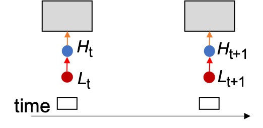
(a) Video SR (S-SR)	(b) Video Interpolation (T-SR)
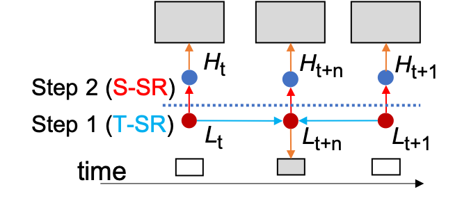
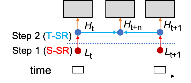
(c) Time-to-Space SR	(d) Space-to-Time SR	(e) Our STARnet

Figure 1: Comparison of SR methods. White and gray rectangles indicate input and output frames, respectively. Small and large rectangles indicate S-LR and S-HR frames, respectively. We omit the feature extraction steps from images to features. (a) and (b) are original S-SR and T-SR methods, respectively. For ST-SR, (c) performs T-SR to produce in-between frames then enlarge the frames using S-SR (e.g., DAIN [3]$\rightarrow$RBPN [17]). The other way around, (d) performs S-SR then the SR frames are used to produce in-between frames using T-SR (e.g., RBPN [17]$\rightarrow$DAIN [3]). Our STARnet (e) jointly optimizes all tasks (S-SR, T-SR, and ST-SR) for augmenting space and time features mutually in multiple resolutions. The purple arrows present direct connections from LR to HR for ST-SR. In addition to upsampling, down-sampling is used to transform S-HR features back to S-LR features for the mutual connection in multiple resolutions.

However, space and time are obviously related. This relation allows us to jointly employ spatial and temporal representations for solving vision tasks on both human [20, 21, 8] and machine perceptions [39, 62, 6, 55, 17, 57, 31]. Intuitively, more accurate motions can be represented on a higher spatial representation and, the other way around, a higher temporal representation (i.e., more frames all of which are similar in appearance) can be used to accurately extract more spatial contexts captured in the temporal frames as done in multi-image SR and video SR. This intuition is also supported by various joint learning problems [18, 15, 61, 1, 60, 56, 29], which are proven to improve learning efficiency and prediction accuracy.

ST-SR
	Input Overlayed	TOFlow$\rightarrow$DBPN	DBPN$\rightarrow$TOFlow	Ours
		[58]       [14]	[14]       [58]
T-SR
	Input Overlayed	TOFlow[58]	DAIN[3]	Ours
S-SR
	Input	DBPN[14]	RBPN[17]	Ours

Figure 2: Comparison on ST-SR, T-SR, and S-SR (S-SR: $4\times$ and T-SR: $2\times$). Red arrows show artifacts and blur produced by other approaches while STARnet (ours) can construct better images.

In order to utilize the complementary nature of space and time, we propose the Space-Time-Aware multiResolution Network, called STARnet. STARnet explicitly incorporates spatial and temporal representations for augmenting S-SR and T-SR mutually in LR and HR spaces by presenting direct connections from LR to HR for ST-SR, indicated as purple arrows in Fig. 1 (e). This network also provides the extensibility where the same network can be further finetuned for either of ST-SR, S-SR, or T-SR. As shown in Fig. 2, STAR-based finetuned models perform better than state-of-the-arts [58, 14, 3, 17].

The main contributions of this paper are as follows:

1) The novel learning-based ST-SR method, which trains a deep network end-to-end to jointly learn spatial and temporal contexts, leading to what we call Space-Time-Aware multiResolution Networks (STARnet). This approach outperforms the combinations of S-SR and T-SR methods.

2) Joint learning on multiple resolutions to estimate both large and subtle motions observed in videos. Performing T-SR on S-HR frames has difficulties in estimating large motions, while subtle motions can be difficult to interpolate on S-LR frames. Our joint learning solves both problems by presenting rich multi-scale features via direct lateral connections between multiple resolutions.

3) A novel view of S-SR and T-SR that are superior to direct S-SR and T-SR. In contrast to the direct S-SR and T-SR approaches, our S-SR and T-SR models are acquired by finetuning STAR. This finetuning from STAR allows the S-SR and T-SR models to be augmented by ST-SR learning; (1) S-SR is augmented by interpolated frames as well as by input frames and (2) T-SR is augmented by subtle motions observed in S-HR as well as large motion observed in S-LR.

2 Related Work

Space SR. Deep SR [9] is extended by better up-sampling layers [51], residual learning [26, 54], back-projection [14, 16], recursive layers [27], and progressive upsampling [30]. In video SR, temporal information is retained by frame concatenation [7, 24] and recurrent networks [22, 46, 17].

Time SR. T-SR, or video interpolation, aims to synthesize in-between frames [36, 45, 23, 35, 42, 41, 3, 43, 37, 59]. The previous methods use a flow image as a motion representation [23, 41, 3, 58, 59]. However, the flow image suffers from blur and large motions. DAIN [3] employed monocular depth estimation in order to support robust flow estimation. As another approach, by spatially downscaling input S-HR frames, large and subtle motions can be extracted in downscaled S-LR and input S-HR frames, respectively [37, 43]. While these methods [37, 43] downscale input S-HR frames for T-SR with joint training of multiple spatial resolutions, STARnet upscales input S-LR frames both in input and interpolated frames for ST-SR with joint training of multiple spatial and temporal resolutions.

Space-Time SR. The first work of ST-SR [49, 50] solved huge linear equations, then created a vector containing all the space-time measurement from all LR frames. Later, [47] presented ST-SR from a single video recording under the assumption of spatial and temporal recurrences. These previous work [49, 50, 47, 32, 40] have several drawbacks, such as dependencies between the equations, its sensitivity to some parameters, and required longer videos to extract meaningful space-time patterns. [48] proposed STSR method to learn LR-HR non-linear mapping. However, it did not investigate the effectiveness of multiple spatial resolutions to improve the ST-SR results. Furthermore, it is also evaluated on a limited test set.

Another approach is to combine S-SR and T-SR, as shown in Fig. 1 (c) and (d). However, this approach treats each context, spatial and temporal, independently. ST-SR has not been investigated thoroughly using joint learning.

3 Space-Time-Aware multiResolution

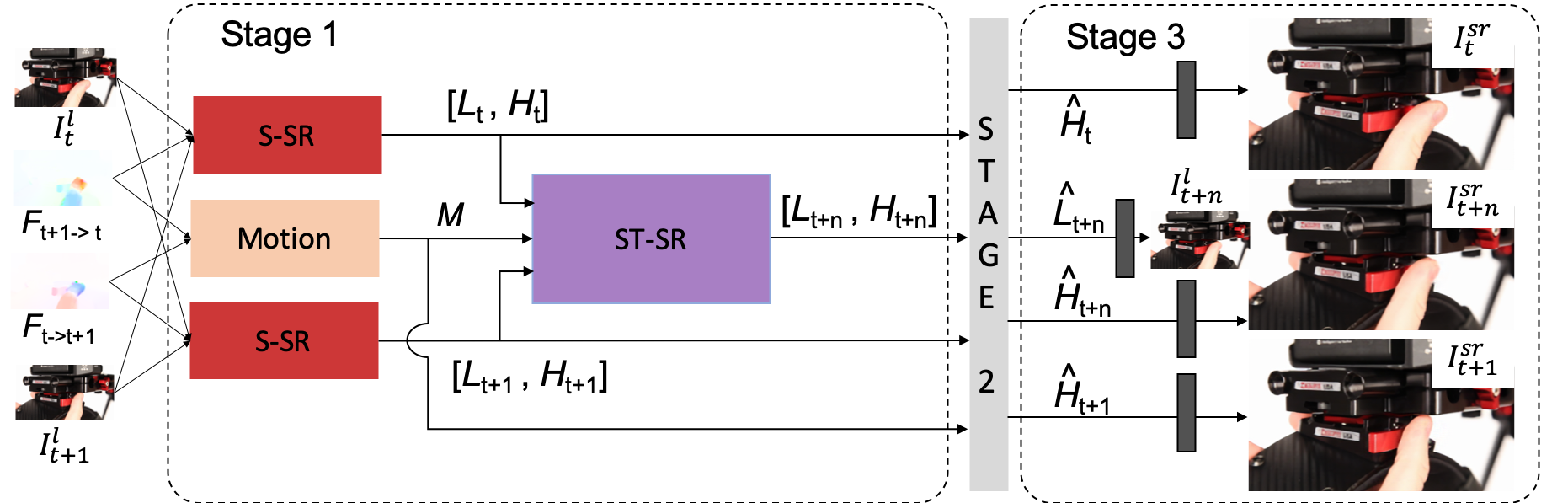
Figure 3: Overview of Space-Time-Aware multiResolution Network (STARnet). First, S-SR produces a pair of S-LR and S-HR feature-maps ($L_{t}$, $H_{t}$, $L_{t+1}$, and $H_{t+1}$) at each time. Motion representation ($M$) is calculated by Motion network from bidirectional optical flow images ($F_{t\rightarrow t{\texttt{+}}1}$ and $F_{t{\texttt{+}}1\rightarrow t}$). With these features, ST-SR produces the feature-maps of the in-between frame ($L_{t+n}$ and $H_{t+n}$). Finally, we reconstruct all outputs of STARnet ($I_{t}^{sr}$, $I_{t+n}^{sr}$, $I_{t+1}^{sr}$, and $I_{t+n}^{l}$) by concatenating all features-maps on LR and HR in space and time.

3.1 Formulation

Given two LR frames ($I^{l}_{t}$ and $I^{l}_{t{\texttt{+}}1}$) with size of $(M^{l}\times N^{l})$, ST-SR obtains space-time SR frames ($I^{sr}_{t},I^{sr}_{t{\texttt{+}}n},I^{sr}_{t{\texttt{+}}1}$) with size of $(M^{h}\times N^{h})$ where $n~{}\in~{}[0,1]$ and $M^{l}<M^{h}$ and $N^{l}<N^{h}$. The goal of ST-SR is to produce $\{I^{sr}_{t}\}_{t=0}^{T\texttt{+}}$ from $\{I^{l}_{1}\}_{t=0}^{T}$, where $T\texttt{+}$ indicates the higher number of frames than $T$. In addition, STARnet computes an in-between S-LR frame ($I^{l}_{t{\texttt{+}}n}$) from ($I^{l}_{t}$ and $I^{l}_{t{\texttt{+}}1}$) for joint learning on LR and HR in space and time. Bidirectional dense motion flow maps, $F_{t\rightarrow t{\texttt{+}}1}$ and $F_{t{\texttt{+}}1\rightarrow t}$ (describing a 2D vector per pixel), between $I^{l}_{t}$ and $I^{l}_{t{\texttt{+}}1}$ are precomputed. Let L${}_{t}~{}\in~{}\mathbb{R}^{M^{l}\times N^{l}\times c^{l}}$ and H${}_{t}~{}\in~{}\mathbb{R}^{M^{h}\times N^{h}\times c^{h}}$ represent the S-LR and S-HR feature-maps on time $t$, respectively, where $c^{l}$ and $c^{h}$ are the number of channels.

STARnet’s operation is divided into three stages: initialization (stage 1), refinement (stage 2), and reconstruction (stage 3); Fig. 3. We train the entire network end-to-end.

Initialization (Stage 1) achieves joint learning of S-SR, T-SR, and ST-SR on LR and HR where T-SR and ST-SR are performed in the same subnetwork indicated by “ST-SR.” This stage takes four inputs: two RGB frames ($I^{l}_{t},I^{l}_{t{\texttt{+}}1}$) and their bidirectional flow images ($F_{t\rightarrow t{\texttt{+}}1},F_{t{\texttt{+}}1\rightarrow t}$). Stage 1 is defined as follows:

$$\text{S-SR:}~{}~{}~{}~{}~{}~{}~{}~{}~{}H_{t}=\texttt{Net}_{S}(I^{l}_{t},I^{l}_{t{\texttt{+}}1},F_{t{\texttt{+}}1\rightarrow t};\theta_{s})$$

$$\hskip 28.00006pt~{}~{}~{}~{}~{}H_{t{\texttt{+}}1}=\texttt{Net}_{S}(I^{l}_{t{\texttt{+}}1},I^{l}_{t},F_{t\rightarrow t{\texttt{+}}1};\theta_{s})$$ (1)

$$\hskip 28.00006pt~{}~{}~{}~{}~{}~{}~{}~{}~{}L_{t}=\texttt{Net}_{D}(H_{t};\theta_{d})$$

$$\hskip 28.00006pt~{}~{}~{}~{}~{}~{}L_{t{\texttt{+}}1}=\texttt{Net}_{D}(H_{t{\texttt{+}}1};\theta_{d})$$ (2)

$$\text{Motion:}~{}~{}~{}~{}~{}~{}~{}~{}M=\texttt{Net}_{M}(F_{t\rightarrow t{\texttt{+}}1},F_{t{\texttt{+}}1\rightarrow t};\theta_{m})$$ (3)

$$\text{ST-SR:}~{}H_{t{\texttt{+}}n},L_{t{\texttt{+}}n}=\texttt{Net}_{ST}(H_{t},H_{t{\texttt{+}}1},L_{t},L_{t{\texttt{+}}1},M;\theta_{st})$$ (4)

In S-SR, S-HR feature-maps ($H_{t}$ and $H_{t+1}$) are produced by $\texttt{Net}_{S}$, as expressed in Eq. (1). As with other video SR methods, this S-SR is performed with sequential frames ($I^{l}_{t}$ and $I^{l}_{t+1}$) and their flow image ($F_{t{\texttt{+}}1\rightarrow t}$ or $F_{t\rightarrow t{\texttt{+}}1}$). $\theta$ denotes a set of weights in each network. Following up- and down-samplings for enhancing features for SR [14, 17], $H_{t}$ and $H_{t+1}$ are downscaled by $\texttt{Net}_{D}$ for updating $L_{t}$ and $L_{t+1}$, respectively, as expressed in Eq. (2). $\texttt{Net}_{M}$ produces a motion representation ($M$) which is calculated from the bidirectional optical flows; Eq. (3). The output of $\texttt{Net}_{M}$ is flow feature maps, learned by a CNN. While it is hard to interpret these features directly, they are intended to help spatial alignment between $F_{t\rightarrow t{\texttt{+}}1}$ and $F_{t{\texttt{+}}1\rightarrow t}$.

Finally, with the concatenation of all these features, ST-SR in the feature space is performed by $\texttt{Net}_{ST}$; Eq. (4). $\texttt{Net}_{ST}$ achieves T-SR as well as ST-SR which are incorporated on LR and HR, shown as blue and purple arrows in Fig. 1 (e). The outputs of stage 1 are HR and LR feature-maps ($H_{t+n}$ and $L_{t+n}$) for an in-between frame.

In this stage, STARnet maintains cycle consistencies (1) between S-HR and S-LR and (2) between $t$ and $t+1$, while such a cycle consistency is demonstrated for general purposes [64, 13, 63],

Refinement (Stage 2) further maintains the cycle consistencies for refining the feature-maps again. While raw optical flows ($F_{t{\texttt{+}}1\rightarrow t}$ and $F_{t\rightarrow t{\texttt{+}}1}$) are used in Eq. (1) of Stage 1, the motion feature ($M$) is used in the first equations of Eqs (5), (7), (9), and (10) in Stage 2. This difference allows us to produce more reliable feature-maps. For further refinement, residual features are extracted in Eqs. (6), (8), and (11), as proposed in RBPN [17] for precise spatial alignment of temporal features.

Finally, Stage 2 is defined as follows:

t: $$H_{t}^{b}~{}=\texttt{Net}_{B}(L_{t{\texttt{+}}n},L_{t},M;\theta_{b})$$

$$L_{t}^{b}~{}=\texttt{Net}_{D}(H_{t}^{b};\theta_{d})$$ (5)

$$\hat{H}_{t}~{}=H_{t}{\texttt{+}}\texttt{ReLU}(H_{t}\texttt{-}H_{t}^{b})$$

$$\hat{L}_{t}~{}=L_{t}{\texttt{+}}\texttt{ReLU}(L_{t}\texttt{-}L_{t}^{b})$$ (6)

t+1: $$H_{t{\texttt{+}}1}^{f}=\texttt{Net}_{F}(L_{t{\texttt{+}}n},L_{t{\texttt{+}}1},M;\theta_{f})$$

$$L_{t{\texttt{+}}1}^{f}=\texttt{Net}_{D}(H_{t{\texttt{+}}1}^{f};\theta_{d})$$ (7)

$$\hat{H}_{t{\texttt{+}}1}~{}=H_{t{\texttt{+}}1}{\texttt{+}}\texttt{ReLU}(H_{t{\texttt{+}}1}\texttt{-}H_{t{\texttt{+}}1}^{f})$$

$$\hat{L}_{t{\texttt{+}}1}~{}=L_{t{\texttt{+}}1}{\texttt{+}}\texttt{ReLU}(L_{t{\texttt{+}}1}\texttt{-}L_{t{\texttt{+}}1}^{f})$$ (8)

t+n: $$H_{t{\texttt{+}}n}^{f}=\texttt{Net}_{F}(\hat{L}_{t},L_{t{\texttt{+}}n},M;\theta_{f})$$

$$L_{t{\texttt{+}}n}^{f}=\texttt{Net}_{D}(H_{t{\texttt{+}}n}^{f};\theta_{d})$$ (9)

$$H_{t{\texttt{+}}n}^{b}=\texttt{Net}_{B}(\hat{L}_{t{\texttt{+}}1},L_{t{\texttt{+}}n},M;\theta_{b})$$

$$L_{t{\texttt{+}}n}^{b}=\texttt{Net}_{D}(H_{t{\texttt{+}}n}^{b};\theta_{d})$$ (10)

$$\hat{H}_{t{\texttt{+}}n}=H_{t{\texttt{+}}n}{\texttt{+}}\texttt{ReLU}(H_{t{\texttt{+}}n}\texttt{-}H_{t{\texttt{+}}n}^{f}){\texttt{+}}\texttt{ReLU}(H_{t{\texttt{+}}n}\texttt{-}H_{t{\texttt{+}}n}^{b})$$

$$\hat{L}_{t{\texttt{+}}n}~{}=L_{t{\texttt{+}}n}{\texttt{+}}\texttt{ReLU}(L_{t{\texttt{+}}n}\texttt{-}L_{t{\texttt{+}}n}^{f}){\texttt{+}}\texttt{ReLU}(L_{t{\texttt{+}}n}\texttt{-}L_{t{\texttt{+}}n}^{b})$$ (11)

Reconstruction (Stage 3) transforms four feature-maps ($\hat{H}_{t}$, $\hat{H}_{t+n}$, $\hat{H}_{t+1}$, and $\hat{L}_{t+n}$) to their corresponding images ($I^{sr}_{t}$, $I^{sr}_{t+n}$, $I^{sr}_{t+1}$, and $I^{l}_{t+n}$) by using only one conv layer $\texttt{Net}_{rec}$; for example, $I^{sr}_{t}~{}=~{}\texttt{Net}_{rec}(\hat{H}_{t};\theta_{rec})$.

3.2 Training Objectives

The reconstructed images of STARnet ($I^{sr}_{t}$, $I^{sr}_{t+n}$, $I^{sr}_{t+1}$, and $I^{l}_{t+n}$) are compared with their ground-truth images by loss functions in a training phase. For this training, (1) S-HR images as the ground-truth images are downscaled to S-LR images and (2) T-HR frames as the ground-truth frames are skimmed to T-LR frames. The loss functions are divided into the following three types:

Space loss

is evaluated on $I^{sr}_{t}$ and $I^{sr}_{t\texttt{+}1}$.

Time loss

is evaluated only on $I^{l}_{t+n}$.

Space-Time loss

is evaluated only on $I^{sr}_{t+n}$.

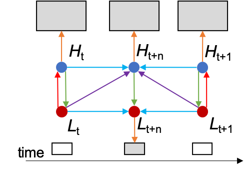
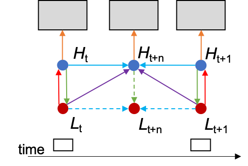
(a) STAR	(b) STAR-ST

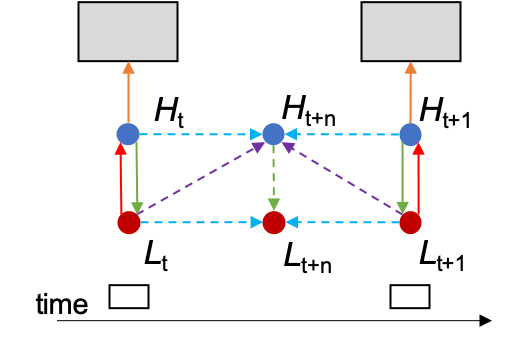
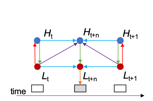
(c) STAR-S	(d) STAR-T

Figure 4: Variants of STARnet train on different training objective for specific tasks. Small and large rectangles indicate low- and high-resolution frames, respectively. White and gray rectangles indicate input and output frames, respectively. Dotted arrows indicated that this computation is not directly optimized.

Our framework provides the following four variants, which are trained with different training objectives.

STAR is trained using all of the aforementioned three losses on LR and HR in space and time. STAR produces $\{I^{sr}_{t}\}_{t=0}^{T\texttt{+}}$ and $\{I^{l}_{t}\}_{t=0}^{T\texttt{+}}$ simultaneously as in Fig. 4 (a).

STAR-ST is a fine-tuned model from STAR using Space and Space-Time losses on HR in space and time. The network is optimized on the space-time super-resolved frames $\{I^{sr}_{t}\}_{t=0}^{T\texttt{+}}$ as in Fig. 4 (b).

STAR-S is a fine-tuned model from STAR using Space loss on S-HR, optimizing only $\{I^{sr}_{t}\}_{t=0}^{T}$ as in Fig. 4 (c).

STAR-T is a fine-tuned model from STAR using Time loss on T-HR as in Fig. 4 (d). STAR-T can be trained on two different regimes, S-LR and S-HR. While STAR-T${}_{\texttt{HR}}$ uses the original frames (S-HR) as input frames, STAR-T${}_{\texttt{LR}}$ uses the downscaled frames (S-LR) as input frames.

3.3 Loss Functions

Each of Space, Time, and Space-Time losses consists of two types of loss functions, $L_{1}$ and $L_{vgg}$. $L_{1}$ is the loss per-pixel between a predicted super-resolved frame ($I^{sr}_{t}$) and its ground-truth HR frame ($I^{h}_{t}$) where $t\in[T]$.

$$\begin{split}L_{1}&=\sum_{t=0}^{T}||I^{h}_{t}\texttt{-}I^{sr}_{t}||_{1}\end{split}$$ (12)

$L_{vgg}$ is calculated in the feature space using a pretrained VGG19 network [52]. For computing $L_{vgg}$, both $I^{h}$ and $I^{sr}$ are mapped into the feature space by differentiable functions $f_{m}$ from the VGG multiple max-pool layer ${(m=5)}$.

$$\begin{split}L_{vgg}&=\sum_{t=0}^{T}||f_{m}(I^{h}_{t})\texttt{-}f_{m}(I^{sr}_{t})||^{2}_{2}\end{split}$$ (13)

$L_{1}$ is for fulfilling standard image quality assessment metrics such as PSNR and validated for SR [42, 5], while $L_{vgg}$ improves visual perception [25, 10]. Based on this fact, only $L_{1}$ or a weighted sum of $L_{1}$ and $L_{vgg}$ is utilized for training STARnet depending on the purpose.

3.4 Flow Refinement

As mentioned in Section 3.1, we use flow images precomputed by [34]. As revealed in many video interpolation papers [36, 45, 23, 35, 42, 41, 3, 43, 37, 59], large motions between $t$ and $t+1$ make video interpolation difficult. Flow noise due to such large motions has a bad effect on the interpolation results. While STARnet suppresses this bad effect by T-SR not only in S-HR but also in S-LR, it is difficult to fully resolve this problem. For further improvement, we propose a simple solution to refine or denoise the flow images, called a Flow Refinement (FR) module.

Let $F_{t\rightarrow t{\texttt{+}}1}$ and $F_{t{\texttt{+}}1\rightarrow t}$ are flow images between frames $I^{l}_{t}$ and $I^{l}_{t{\texttt{+}}1}$ on forward and backward motions, respectively. During training, $F_{t\rightarrow t+n}$ can be calculated from an input frame at $t$ to the ground truth (i.e., from $I^{l}_{t}$ to $I^{l}_{t\texttt{+}n}$). $\texttt{Net}_{flow}$ is a U-Net which defines as follows.

$$\begin{split}\text{FR: }&\hat{F}_{t\rightarrow t{\texttt{+}}1}=\texttt{Net}_{flow}(F_{t\rightarrow t{\texttt{+}}1},I_{t},I_{t{\texttt{+}}1};\theta_{flow})\\ &\hat{F}_{t{\texttt{+}}1\rightarrow t}=\texttt{Net}_{flow}(F_{t{\texttt{+}}1\rightarrow t},I_{t{\texttt{+}}1},I_{t};\theta_{flow})\end{split}$$ (14)

To reduce the noise, we propose the following flow refinement loss.

$$\begin{split}L_{flow}=&~{}~{}||\hat{F}_{t\rightarrow t{\texttt{+}}1}\texttt{-}(F_{t\rightarrow t{\texttt{+}}n}{\texttt{+}}F_{t{\texttt{+}}n\rightarrow t{\texttt{+}}1})||^{2}_{2}\\ &{\texttt{+}}||\hat{F}_{t{\texttt{+}}1\rightarrow t}\texttt{-}(F_{t{\texttt{+}}1\rightarrow t{\texttt{+}}n}{\texttt{+}}F_{t{\texttt{+}}n\rightarrow t})||^{2}_{2}\end{split}$$ (15)

With $L_{flow}$, the loss functions for training STARnet are defined as follows:

$$L_{r} = w_{1}*L_{1}{\texttt{+}}w_{2}*L_{flow}$$ (16)

$$L_{f} = L_{r}{\texttt{+}}w_{3}*L_{vgg}$$ (17)

4 Experimental Results

In all experiments, we focus on $4\times$ SR factor and $n=0.5$. $I^{sr}_{t}$ and $I^{sr}_{t\texttt{+}}$ denote the SR frames of input frames and in-between frames, respectively.

4.1 Implementation Details

Stage 1. For $\texttt{Net}_{S}$ and $\texttt{Net}_{D}$, we use DBPN [14] or RBPN [17] that have up- and down-sampling layers to simultaneously produce a pair of S-LR and S-HR features with $c^{h}$=64 and $c^{l}$=128. $\texttt{Net}_{M}$ is constructed with two residual blocks where each block consists of two conv layers with $3\times 3$ with stride = 1 and pad by 1. $\texttt{Net}_{ST}$ has five residual blocks followed by deconv layers for upsampling.

Stage 2. Both $\texttt{Net}_{F}$ and $\texttt{Net}_{B}$ are constructed using five residual blocks and deconv layers.

Train Dataset. We use the triplet training set in Vimeo90K [58] for training. This dataset has 51,313 triplets from 14,777 video clips with a fixed resolution, $448\times 256$. During training, we apply augmentation, such as rotation, flipping, and random cropping. The original images are regarded as S-HR and downscaled to $112\times 64$ S-LR frames ($4\times$ smaller than the originals) with Bicubic interpolation.

Test Dataset and Metrics. We evaluate our method on several test sets. The test set of Vimeo90K [58] consists of 3,782 triplets with the original resolution of $448\times 256$ pixels. While UCF101 [53] is developed for action recognition, it is also used for evaluating T-SR methods. This test set consists of 379 triplets with the original resolution of $256\times 256$ pixels. Middlebury [2] has the original resolution of $640\times 480$ pixels. We evaluate PSNR, SSIM, and interpolation error (IE) on the test sets.

Training Strategy. The batch size is 10 with $112\times 64$ pixels (S-LR scale). The learning rate is initialized to $1e-4$ for all layers and decreased by a factor of 10 on every 30 epochs for total 70 epochs. For each finetuned model, we use another 20 epochs with learning rate $1e-4$ and decreased by a factor of 10 on every 10 epochs. We initialize the weights based on [19]. For optimization, we used AdaMax [28] with momentum to $0.9$. All experiments were conducted using Python 3.5.2 and PyTorch 1.0 on NVIDIA Tesla V100 GPUs. For the loss setting, we use $w_{1}$: 1, $w_{2}$: 0.1, and $w_{3}$: 0.1.

4.2 Ablation Studies

Here, we evaluate STARnet without T-SR paths (blue arrows in Fig. 1 (e)) in order to clarify the effectiveness our core contribution (i.e., joint learning in time and space on multiple resolutions) with a simplified network using direct ST-SR paths (purple arrows). The test set of Vimeo90K [58] is used.

Basic components. We evaluate the basic components on STARnet. In the first experiment, we remove the refinement part (i.e., Stage 2), leaving only the initialization part. Second, we omit input flow images and $\texttt{Net}_{M}$, so no motion context is used (STAR w/o Flow). Third, the FR module is removed. Finally, the full model is evaluated. The results of these four models are shown in “STAR w/o Stage 2,” “STAR w/o Flow,” “STAR w/o FR,” and “STAR” in Table 1. Compared with the full model, the PSNR of STAR w/o Stage 2 decreases to 0.36dB and 1.0dB on $I^{sr}_{t\texttt{+}}$ and $I^{sr}_{t}$, respectively. The flow information can also improve the PSNR 0.28dB and 0.43dB on $I^{sr}_{t\texttt{+}}$ and $I^{sr}_{t}$, respectively.

While FR is also useful, the quantitative improvement by FR is not substantial compared with those of the other two components. The examples of $I^{sr}_{t\texttt{+}}$ are shown in Fig. 5 where flow images are computed only by $I^{l}_{t}$ and $I^{l}_{t+1}$, only by $I^{l}_{t}$ and $I^{l}_{t+1}$ and refined by FR, and by $I^{l}_{t\texttt{+}}$ (i.e., GT in-between frame) in addition to $I^{l}_{t}$ and $I^{l}_{t+1}$ in (a), (b), and (c), respectively. In Fig. 5, the visual improvement by FR is substantial. This result reveals that (1) erroneous flows are critical for generating $I^{sr}_{t\texttt{+}}$ (i.e., for ST-SR) and (2) FR can rectify the flow image significantly on several images.

	$I^{sr}_{t}$		$I^{sr}_{t\texttt{+}}$
Method	PSNR	SSIM	PSNR	SSIM
STAR w/o Stage 2	30.920	0.921	30.002	0.917
STAR w/o Flow	31.489	0.928	30.086	0.918
STAR w/o FR	31.601	0.929	30.229	0.920
STAR	31.920	0.933	30.365	0.923

Table 1: Baseline comparison of STAR with DBPN [16] and $L_{f}$. Red in all tables indicates the best performance.

	Image 1				Image 2
PSNR: 22.68dB	PSNR: 23.48dB	PSNR: 24.26dB		PSNR: 18.59dB	PSNR: 19.19dB	PSNR: 20.29dB
(a) w/o FR	(b) w/ FR	(c) GT Flow		(a) w/o FR	(b) w/ FR	(c) GT Flow

Figure 5: Visual analysis of $I^{sr}_{t\texttt{+}}$ with and w/o FR. (a) Flows are computed by $I^{l}_{t}$ and $I^{l}_{t+1}$. (b) Flows are computed by $I^{l}_{t}$ and $I^{l}_{t+1}$ and refined by FR. (c) Flows are computed by $I^{l}_{t\texttt{+}}$ (i.e., GT in-between frame) in addition to $I^{l}_{t}$ and $I^{l}_{t+1}$

Training Objectives. Table 2 shows that finetuning STAR to STAR-ST, STAR-S, and STAR-T is beneficial for improving ST-SR, S-SR, and T-SR, respectively.

	$I^{sr}_{t}$		$I^{sr}_{t\texttt{+}}$		$I^{l}_{t\texttt{+}}$
Method	PSNR	SSIM	PSNR	SSIM	PSNR	SSIM
STAR	31.601	0.929	30.229	0.920	39.014	0.990
STAR-ST	31.883	0.933	30.350	0.928	NA	NA
STAR-S	32.026	0.935	NA	NA	NA	NA
STAR-T	NA	NA	NA	NA	39.028	0.990

Table 2: Analysis on different training objectives using STARnet with DBPN [16] and $L_{f}$.

Loss Functions. We investigate optimizability of two losses, Eqs. (16) and (17), as shown in Table 3. The results show that $L_{r}$ increases the PSNR by 0.19dB and 0.16dB on $I^{sr}_{t}$ and $I^{sr}_{t\texttt{+}}$, respectively. However, $L_{f}$ has a better NIQE score, which shows that this loss perceives better human perception. In what follows, $L_{r}$ is used.

	$I^{sr}_{t}$			$I^{sr}_{t\texttt{+}}$
Loss	PSNR	SSIM	NIQE [38]	PSNR	SSIM	NIQE [38]
$L_{f}$	32.153	0.936	6.288	30.545	0.925	6.289
$L_{r}$	32.349	0.938	6.905	30.704	0.928	6.942

Table 3: Analysis on two loss functions using STAR-ST with RBPN. Higher PSNR and SSIM indicate better results, while a lower NIQE indicates a better perceptual index.

S-SR module. We compare two S-SR methods, DBPN [16] for single-image SR and RBPN [17] for video SR, as the S-SR module in Stage 1; Table 4. RBPN can work better in all cases.

	$I^{sr}_{t}$		$I^{sr}_{t\texttt{+}}$
Method	PSNR	SSIM	PSNR	SSIM
STAR with DBPN [16]	32.160	0.936	30.540	0.925
STAR with RBPN [17]	32.349	0.938	30.704	0.928

Table 4: Analysis on the S-SR module using STAR-ST and $L_{r}$.

Larger scale T-SR. The performance on a larger scale T-SR is investigated. While the S-SR factor is the same with that in other experiments (i.e., 4$\times$), the frame-rate is upscaled to 4$\times$. We compare two upscaling paths: (1) STAR-ST (2$\times$ S-SR and 2$\times$ T-SR) $\rightarrow$ STAR-ST (2$\times$ S-SR and 2$\times$ T-SR) (2) STAR-ST (4$\times$ S-SR and 2$\times$ T-SR) $\rightarrow$ STAR-T (2$\times$ T-SR). For training 4$\times$ T-SR, the training set of the Vimeo90K setuplet, where each sequence has 7 frames, is used. Then, the 1st and 5th frames in the Vimeo90K setuplet test set are used as input frames for evaluation. As shown in in Table 5, the second path is better. This result may suggest that a higher spatial resolution provides better results on T-SR.

	$I^{sr}_{t}$		$I^{sr}_{t\texttt{+}}$
Method	PSNR	SSIM	PSNR	SSIM
(1) STAR-ST $\rightarrow$ STAR-ST	33.007	0.941	27.186	0.893
(2) STAR-ST $\rightarrow$ STAR-T	34.146	0.950	27.640	0.901

Table 5: Analysis on larger scale T-SR (4$\times$) on the Vimeo90K setuplet test set with $L_{r}$.

	$I^{sr}_{t}$		$I^{sr}_{t\texttt{+}}$
Method	PSNR	SSIM	PSNR	SSIM
(1) Only ST-SR	32.349	0.938	30.704	0.928
(2) ST-SR+T-SRS-HR	32.398	0.939	30.712	0.928
(3) ST-SR+T-SRS-LR	32.421	0.939	30.760	0.928
(4) Full	32.547	0.940	30.830	0.929

Table 6: Analysis on ST-SR jointly trained with T-SR with RBPN [17] and $L_{r}$. Models are optimized for STAR-ST w/ FR.

T-SR paths on S-HR and S-LR domains. We analyze the effectiveness of T-SR on multiple spatial resolutions (blue arrows in Fig. 1 (e)) as well as ST-SR (purple arrows in Fig. 1 (e)). Table 6 shows the results of the following four experiments. In (1), we remove all T-SR modules (blue arrows). In (2), T-SR on S-HR is incorporated with ST-SR module. In (3), T-SR on S-LR is incorporated with ST-SR module. In (4), all modules are used as shown in Fig. 1 (e). In these implementations, T-SR modules can be removed by modifying $\texttt{Net}_{ST}$ in Eq. (4) so that it contains only ST-SR, ST-SR+T-SR_S-HR, ST-SR+T-SR_S-LR, and all of them for (1), (2), (3), and (4), respectively. It confirms that joint training of ST-SR and T-SR improves the performance. Both S-HR and S-LR resolutions improve the performance compared with only ST-SR, while the best results are obtained by the full STAR model.

	UCF101 [53]			Vimeo90K [58]			Middlebury (Other) [2]
Method	PSNR	SSIM	NIQE	PSNR	SSIM	NIQE	PSNR	SSIM	NIQE
ToFlow [58] $\rightarrow$ DBPN [16]	27.228	0.885	9.123	28.821	0.897	7.758	24.984	0.790	6.473
DBPN [16] $\rightarrow$ ToFlow [58]	28.112	0.902	8.630	29.867	0.915	7.120	26.012	0.808	5.801
DBPN [16] $\rightarrow$ DAIN [3]	28.175	0.902	8.755	30.021	0.918	7.223	26.268	0.809	5.869
DBPN-MI $\rightarrow$ DAIN [3]	28.578	0.916	8.922	30.286	0.923	7.218	26.447	0.815	5.702
DAIN [3] $\rightarrow$ RBPN [17]	27.631	0.909	8.932	29.422	0.916	7.253	25.744	0.811	5.814
RBPN [17] $\rightarrow$ DAIN [3]	28.729	0.919	8.769	30.455	0.926	7.081	26.766	0.821	5.522
RBPN [17] $\rightarrow$ DAIN [3]	28.856	0.920	8.799	30.623	0.927	7.183	26.923	0.823	5.444
STAR-$L_{f}$	28.829	0.920	7.875	30.608	0.926	6.251	26.881	0.824	4.579
STAR-ST-$L_{f}$	28.806	0.920	7.868	30.714	0.927	6.470	27.020	0.826	4.802
STAR-ST-$L_{r}$	29.111	0.924	8.787	30.830	0.929	7.154	27.115	0.827	5.423

Table 7: Comparison on ST-SR ($I^{sr}_{t\texttt{+}})$ using $L_{r}$. $\alpha\rightarrow\beta$ indicates the output of $\alpha$ is the input of $\beta$. Red indicates the best and blue indicates the second best performance in all tables in Section 4.3. * indicates a joint learning of RBPN and DAIN methods to perform ST-SR.

4.3 Comparisons with State-of-the-art

The following results are obtained by the full STAR model, which is evaluated as the best in Table 6.

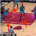
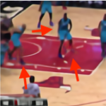
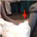
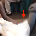
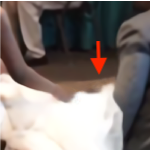
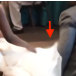
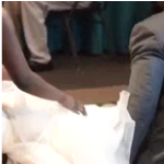
(a)	(b)	(c)	(d)	(d)
DBPN [16]$\rightarrow$ToFlow [58]	DAIN [3]$\rightarrow$RBPN [17]	RBPN [17]$\rightarrow$DAIN [3]	STAR-ST	GT

Figure 6: Visual results on ST-SR ($I^{sr}_{t\texttt{+}}$). Red arrows here and in the other figures indicates the highlighted area.

	UCF101		Vimeo90K
Method	PSNR	SSIM	PSNR	SSIM
Bicubic	27.217	0.887	28.134	0.878
DBPN [16]	29.828	0.913	31.505	0.927
DBPN-MI	30.666	0.934	31.835	0.933
RBPN [17]	30.969	0.938	32.154	0.936
STAR-ST	31.532	0.942	32.547	0.940
STAR-S	31.604	0.943	32.702	0.941

Table 8: Comparison on S-SR ($I^{sr}_{t}$) using $L_{r}$.

	UCF101 [53]		Vimeo90K [58]		Middlebury [2]
					Other	*Eval
Method	PSNR	SSIM	PSNR	SSIM	IE	IE
SPyNet [44]	33.67	0.963	31.95	0.960	2.49	-
EpicFlow [45]	33.71	0.963	32.02	0.962	2.47	-
MIND [36]	33.93	0.966	33.50	0.943	3.35	-
DVF [35]	34.12	0.963	31.54	0.946	7.75	-
ToFlow [58]	34.58	0.967	33.73	0.968	2.51	5.49
SepConv-Lf [42]	34.69	0.965	33.45	0.967	2.44	-
SepConv-L1 [42]	34.78	0.967	33.79	0.970	2.27	5.61
MEMC-Net [4]	34.96	0.968	34.29	0.974	2.12	4.99
DAIN [3]	34.99	0.968	34.71	0.976	2.04	4.86
STAR	34.78	0.964	33.11	0.957	2.41	-
STAR-T${}_{\text{LR}}$	34.80	0.964	33.19	0.958	2.36	-
STAR-T${}_{\text{HR}}$	35.07	0.967	35.11	0.976	1.95	4.70

Table 9: Comparison on T-SR on the original resolution. SSIM is almost saturated especially on UCF101, so PSNR is a better measure here. *Results are taken from Middlebury dashboard.

Methods	ToFlow [58]	DAIN [3]	STAR	STAR-T${}_{\text{HR}}$	STAR-T${}_{\text{LR}}$
PSNR	36.04	36.69	39.13	38.60	39.30
SSIM	0.984	0.986	0.991	0.990	0.991

Table 10: Comparison of T-SR on L-SR ($I^{l}_{t\texttt{+}}$) with Vimeo90K [58].

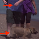
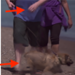
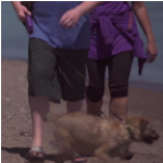
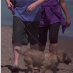
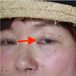
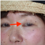
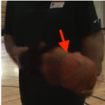
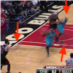
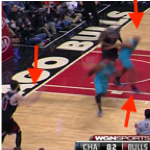
(a)	(b)	(c)	(d)
ToFlow [58]	DAIN [3]	STAR-T	GT

Figure 7: Visual results on T-SR on the original resolution.

ST-SR. As discussed in Section 2, older ST-SR methods [49, 50, 47, 32, 40] cannot be applied to videos in the Vimeo90K dataset. We can combine more modern S-SR and T-SR methods to perform ST-SR. We use DBPN [16] and RBPN [17] as S-SR. For T-SR, we choose ToFlow [58] and DAIN [3]. In Table 7, we present the results of ST-SR obtained by six combinations of these methods.

It is found that S-SR$\rightarrow$T-SR performs better than T-SR$\rightarrow$S-SR. The margin is up to 1dB on Vimeo90K, showing that the performance of previous T-SRs significantly drops on LR images. Even STAR is better than the combination of state-of-the-arts (RBPN [17]$\rightarrow$DAIN [3]), while the best result is achieved by STAR-ST, which is the finetuned model from STAR. STAR-ST has a better performance around 0.38dB than RBPN [17]$\rightarrow$DAIN [3] on Vimeo90K test set.

We can also present ST-SR as a joint learning of RBPN [17] and DAIN [3], indicated as (*). It shows that joint learning is effective to improve this combination as well as STAR. However, STAR, which leverages direct connections for ST-SR (i.e., purple arrows in Fig. 1 (e)) and joint learning in space and time, shows the best performance. Visual results shown in Fig. 6 demonstrate that STAR-ST produces sharper images than others.

S-SR. The results on S-SR are shown in Table 8. Our methods are compared with DBPN [16], DBPN-MI, and RBPN [17]. DBPN is a single image SR method. A Multi-Image extension of DBPN (DBPN-MI) uses DBPN with a temporal concatenation of RGB and optical flow images. DBPN-MI and RBPN have the same input regimes using sequential frames and optical flow images.

It shows that multiple frames are able to improve the performance of DBPN for around 0.3dB on Vimeo90K. RBPN successfully leverages temporal connections of sequential frames for performance improvement compared with DBPN and DBPN-MI. As expected, STAR-S is the best, which is also better than STAR-ST. It can improve the PSNR by 1.19dB dB, 0.87dB, and 0.55dB compared with DBPN [16], DBPN-MI, and RBPN [17], respectively, on Vimeo90K test set.

T-SR. Our method is compared with eight state-of-the-art T-SR methods: SPyNet [44], EpicFlow [45], MIND [36], DVF [35], ToFlow [58], SepConv [42], MEMC-Net [4], and DAIN [3]. Input frames are the original size of the test set without downscaling. As shown in Table 9, STAR-T${}_{\texttt{HR}}$ is comparable with the state-of-the-art T-SR methods.

The visual results are shown in Fig. 7. We can see that STAR produces better interpolation on subtle and large motions, and also sharper textures. DAIN [3] and ToFlow [58] tend to produce blur images on subtle and large motion areas as shown by the red arrows.

We also investigate the performance on S-LR. There are different motion magnitudes between S-HR and S-LR. Naturally, when the frames are downscaled, the magnitude of pixel displacements is reduced as well. Therefore, each spatial resolution has a different access to the motion variance. The evaluation on S-LR images focuses on subtle motions, while S-HR images focus on large motions. Table 9 shows that STAR-T${}_{\texttt{HR}}$ is superior to STAR-T${}_{\texttt{LR}}$ and other methods on S-HR (original size). Likewise, STAR-T${}_{\texttt{LR}}$ is superior than STAR-T${}_{\texttt{HR}}$ on S-LR (original frames are downscaled ${\downarrow}$ with Bicubic) as shown in Table 10. It shows that if we finetune the network on the same domain, it can increase the performance. Furthermore, we can see that STAR-T${}_{\texttt{LR}}$ is much superior than ToFlow and DAIN.

5 Conclusion

We proposed a novel approach to space-time super-resolution (ST-SR) using a deep network called Space-Time-Aware multiResolution Network (STARnet). The network super-resolves jointly in space and time. We show that a higher resolution presents detailed motions, while a higher frame-rate provides better pixel alignment. Furthermore, we demonstrate a special mechanism to improve the performance for just S-SR and T-SR. We conclude that the integration of spatial and temporal contexts is able to improve the performance of S-SR, T-SR, and ST-SR by substantial margin on publicly available datasets.

This work was supported by JSPS KAKENHI Grant Number 19K12129.

References

- [1] Yancheng Bai, Yongqiang Zhang, Mingli Ding, and Bernard Ghanem. Finding tiny faces in the wild with generative adversarial network. CVPR. IEEE, 2018.
- [2] Simon Baker, Daniel Scharstein, JP Lewis, Stefan Roth, Michael J Black, and Richard Szeliski. A database and evaluation methodology for optical flow. International Journal of Computer Vision, 92(1):1–31, 2011.
- [3] Wenbo Bao, Wei-Sheng Lai, Chao Ma, Xiaoyun Zhang, Zhiyong Gao, and Ming-Hsuan Yang. Depth-aware video frame interpolation. In CVPR, 2019.
- [4] Wenbo Bao, Wei-Sheng Lai, Xiaoyun Zhang, Zhiyong Gao, and Ming-Hsuan Yang. Memc-net: Motion estimation and motion compensation driven neural network for video interpolation and enhancement. arXiv preprint arXiv:1810.08768, 2018.
- [5] Yochai Blau, Roey Mechrez, Radu Timofte, Tomer Michaeli, and Lihi Zelnik-Manor. 2018 pirm challenge on perceptual image super-resolution. arXiv preprint arXiv:1809.07517, 2018.
- [6] Fabian Caba Heilbron, Juan Carlos Niebles, and Bernard Ghanem. Fast temporal activity proposals for efficient detection of human actions in untrimmed videos. In CVPR, pages 1914–1923, 2016.
- [7] Jose Caballero, Christian Ledig, Andrew P Aitken, Alejandro Acosta, Johannes Totz, Zehan Wang, and Wenzhe Shi. Real-time video super-resolution with spatio-temporal networks and motion compensation. In CVPR, 2017.
- [8] Zhenguang G Cai, Ruiming Wang, Manqiong Shen, and Maarten Speekenbrink. Cross-dimensional magnitude interactions arise from memory interference. Cognitive psychology, 106:21–42, 2018.
- [9] Chao Dong, Chen Change Loy, Kaiming He, and Xiaoou Tang. Image super-resolution using deep convolutional networks. IEEE transactions on pattern analysis and machine intelligence, 38(2):295–307, 2016.
- [10] Alexey Dosovitskiy and Thomas Brox. Generating images with perceptual similarity metrics based on deep networks. In Advances in Neural Information Processing Systems, pages 658–666, 2016.
- [11] Esmaeil Faramarzi, Dinesh Rajan, and Marc P Christensen. Unified blind method for multi-image super-resolution and single/multi-image blur deconvolution. IEEE Transactions on Image Processing, 22(6):2101–2114, 2013.
- [12] Diogo C Garcia, Camilo Dorea, and Ricardo L de Queiroz. Super resolution for multiview images using depth information. IEEE Transactions on Circuits and Systems for Video Technology, 22(9):1249–1256, 2012.
- [13] Clément Godard, Oisin Mac Aodha, and Gabriel J Brostow. Unsupervised monocular depth estimation with left-right consistency. In CVPR, pages 270–279, 2017.
- [14] Muhammad Haris, Greg Shakhnarovich, and Norimichi Ukita. Deep back-projection networks for super-resolution. In CVPR, 2018.
- [15] Muhammad Haris, Greg Shakhnarovich, and Norimichi Ukita. Task-driven super resolution: Object detection in low-resolution images. arXiv preprint arXiv:1803.11316, 2018.
- [16] Muhammad Haris, Greg Shakhnarovich, and Norimichi Ukita. Deep back-projection networks for single imaage super-resolution. arXiv preprint arXiv:1904.05677, 2019.
- [17] Muhammad Haris, Greg Shakhnarovich, and Norimichi Ukita. Recurrent back-projection network for video super-resolution. In CVPR, 2019.
- [18] Kaiming He, Georgia Gkioxari, Piotr Dollár, and Ross Girshick. Mask r-cnn. In ICCV, pages 2961–2969, 2017.
- [19] Kaiming He, Xiangyu Zhang, Shaoqing Ren, and Jian Sun. Delving deep into rectifiers: Surpassing human-level performance on imagenet classification. In ICCV, pages 1026–1034, 2015.
- [20] Chizuru T Homma and Hiroshi Ashida. What makes space-time interactions in human vision asymmetrical? Frontiers in psychology, 6:756, 2015.
- [21] Chizuru T Homma and Hiroshi Ashida. Temporal cognition can affect spatial cognition more than vice versa: The effect of task-related stimulus saliency. Multisensory Research, 1(aop):1–20, 2018.
- [22] Yan Huang, Wei Wang, and Liang Wang. Bidirectional recurrent convolutional networks for multi-frame super-resolution. In Advances in Neural Information Processing Systems, pages 235–243, 2015.
- [23] Huaizu Jiang, Deqing Sun, Varun Jampani, Ming-Hsuan Yang, Erik Learned-Miller, and Jan Kautz. Super slomo: High quality estimation of multiple intermediate frames for video interpolation. In CVPR, pages 9000–9008, 2018.
- [24] Younghyun Jo, Seoung Wug Oh, Jaeyeon Kang, and Seon Joo Kim. Deep video super-resolution network using dynamic upsampling filters without explicit motion compensation. In CVPR, pages 3224–3232, 2018.
- [25] Justin Johnson, Alexandre Alahi, and Li Fei-Fei. Perceptual losses for real-time style transfer and super-resolution. In ECCV, pages 694–711. Springer, 2016.
- [26] Jiwon Kim, Jung Kwon Lee, and Kyoung Mu Lee. Accurate image super-resolution using very deep convolutional networks. In CVPR, pages 1646–1654, June 2016.
- [27] Jiwon Kim, Jung Kwon Lee, and Kyoung Mu Lee. Deeply-recursive convolutional network for image super-resolution. In CVPR, pages 1637–1645, 2016.
- [28] Diederik P Kingma and Jimmy Ba. Adam: A method for stochastic optimization. In ICLR, 2015.
- [29] Alexander Kirillov, Kaiming He, Ross Girshick, Carsten Rother, and Piotr Dollár. Panoptic segmentation. In CVPR, pages 9404–9413, 2019.
- [30] Wei-Sheng Lai, Jia-Bin Huang, Narendra Ahuja, and Ming-Hsuan Yang. Deep laplacian pyramid networks for fast and accurate super-resolution. In CVPR, 2017.
- [31] Colin Lea, Austin Reiter, René Vidal, and Gregory D Hager. Segmental spatiotemporal cnns for fine-grained action segmentation. In ECCV, pages 36–52. Springer, 2016.
- [32] Tao Li, Xiaohai He, Qizhi Teng, Zhengyong Wang, and Chao Ren. Space–time super-resolution with patch group cuts prior. Signal Processing: Image Communication, 30:147–165, 2015.
- [33] Renjie Liao, Xin Tao, Ruiyu Li, Ziyang Ma, and Jiaya Jia. Video super-resolution via deep draft-ensemble learning. In ICCV, pages 531–539, 2015.
- [34] Ce Liu et al. Beyond pixels: exploring new representations and applications for motion analysis. PhD thesis, Massachusetts Institute of Technology, 2009.
- [35] Ziwei Liu, Raymond A Yeh, Xiaoou Tang, Yiming Liu, and Aseem Agarwala. Video frame synthesis using deep voxel flow. In ICCV, pages 4463–4471, 2017.
- [36] Gucan Long, Laurent Kneip, Jose M Alvarez, Hongdong Li, Xiaohu Zhang, and Qifeng Yu. Learning image matching by simply watching video. In ECCV, pages 434–450. Springer, 2016.
- [37] Simone Meyer, Abdelaziz Djelouah, Brian McWilliams, Alexander Sorkine-Hornung, Markus Gross, and Christopher Schroers. Phasenet for video frame interpolation. In CVPR, pages 498–507, 2018.
- [38] Anish Mittal, Rajiv Soundararajan, and Alan C Bovik. Making a” completely blind” image quality analyzer. IEEE Signal Process. Lett., 20(3):209–212, 2013.
- [39] Lichao Mou, Lorenzo Bruzzone, and Xiao Xiang Zhu. Learning spectral-spatial-temporal features via a recurrent convolutional neural network for change detection in multispectral imagery. IEEE Transactions on Geoscience and Remote Sensing, 57(2):924–935, 2019.
- [40] Uma Mudenagudi, Subhashis Banerjee, and Prem Kumar Kalra. Space-time super-resolution using graph-cut optimization. IEEE Transactions on Pattern Analysis and Machine Intelligence, 33(5):995–1008, 2010.
- [41] Simon Niklaus and Feng Liu. Context-aware synthesis for video frame interpolation. In CVPR, pages 1701–1710, 2018.
- [42] Simon Niklaus, Long Mai, and Feng Liu. Video frame interpolation via adaptive separable convolution. In ICCV, pages 261–270, 2017.
- [43] Tomer Peleg, Pablo Szekely, Doron Sabo, and Omry Sendik. Im-net for high resolution video frame interpolation. In CVPR, pages 2398–2407, 2019.
- [44] Anurag Ranjan and Michael J Black. Optical flow estimation using a spatial pyramid network. In CVPR, pages 4161–4170, 2017.
- [45] Jerome Revaud, Philippe Weinzaepfel, Zaid Harchaoui, and Cordelia Schmid. Epicflow: Edge-preserving interpolation of correspondences for optical flow. In CVPR, pages 1164–1172, 2015.
- [46] Mehdi SM Sajjadi, Raviteja Vemulapalli, and Matthew Brown. Frame-recurrent video super-resolution. In CVPR, pages 6626–6634, 2018.
- [47] Oded Shahar, Alon Faktor, and Michal Irani. Super-resolution from a single video. In CVPR, 2011.
- [48] Manoj Sharma, Santanu Chaudhury, and Brejesh Lall. Space-time super-resolution using deep learning based framework. In ICPRML, 2017.
- [49] Eli Shechtman, Yaron Caspi, and Michal Irani. Increasing space-time resolution in video. In ECCV, pages 753–768. Springer, 2002.
- [50] Eli Shechtman, Yaron Caspi, and Michal Irani. Space-time super-resolution. IEEE Transactions on Pattern Analysis & Machine Intelligence, 27(4):531–545, 2005.
- [51] Wenzhe Shi, Jose Caballero, Ferenc Huszár, Johannes Totz, Andrew P Aitken, Rob Bishop, Daniel Rueckert, and Zehan Wang. Real-time single image and video super-resolution using an efficient sub-pixel convolutional neural network. In CVPR, pages 1874–1883, 2016.
- [52] Karen Simonyan and Andrew Zisserman. Very deep convolutional networks for large-scale image recognition. ICLR, 2015.
- [53] Khurram Soomro, Amir Roshan Zamir, and Mubarak Shah. Ucf101: A dataset of 101 human actions classes from videos in the wild. arXiv preprint arXiv:1212.0402, 2012.
- [54] Ying Tai, Jian Yang, and Xiaoming Liu. Image super-resolution via deep recursive residual network. In CVPR, 2017.
- [55] Yi-Hsuan Tsai, Ming-Hsuan Yang, and Michael J Black. Video segmentation via object flow. In CVPR, pages 3899–3908, 2016.
- [56] Qiang Wang, Li Zhang, Luca Bertinetto, Weiming Hu, and Philip HS Torr. Fast online object tracking and segmentation: A unifying approach. In CVPR, pages 1328–1338, 2019.
- [57] Wenguan Wang, Jianbing Shen, and Fatih Porikli. Saliency-aware geodesic video object segmentation. In CVPR, pages 3395–3402, 2015.
- [58] Tianfan Xue, Baian Chen, Jiajun Wu, Donglai Wei, and William T Freeman. Video enhancement with task-oriented flow. International Journal of Computer Vision (IJCV), 127(8):1106–1125, 2019.
- [59] Liangzhe Yuan, Yibo Chen, Hantian Liu, Tao Kong, and Jianbo Shi. Zoom-in-to-check: Boosting video interpolation via instance-level discrimination. In CVPR, pages 12183–12191, 2019.
- [60] Amir R Zamir, Alexander Sax, William Shen, Leonidas J Guibas, Jitendra Malik, and Silvio Savarese. Taskonomy: Disentangling task transfer learning. In CVPR, pages 3712–3722, 2018.
- [61] Yongqiang Zhang, Yancheng Bai, Mingli Ding, and Bernard Ghanem. Sod-mtgan: Small object detection via multi-task generative adversarial network. In ECCV, pages 206–221, 2018.
- [62] Shifu Zhou, Wei Shen, Dan Zeng, Mei Fang, Yuanwang Wei, and Zhijiang Zhang. Spatial–temporal convolutional neural networks for anomaly detection and localization in crowded scenes. Signal Processing: Image Communication, 47:358–368, 2016.
- [63] Tinghui Zhou, Philipp Krahenbuhl, Mathieu Aubry, Qixing Huang, and Alexei A Efros. Learning dense correspondence via 3d-guided cycle consistency. In CVPR, pages 117–126, 2016.
- [64] Jun-Yan Zhu, Taesung Park, Phillip Isola, and Alexei A Efros. Unpaired image-to-image translation using cycle-consistent adversarial networks. In ICCV, pages 2223–2232, 2017.