$\Lambda$CDM as a Noether Symmetry in Cosmology

Abstract

The standard $\Lambda$CDM model of cosmology is formulated as a simple modified gravity coupled to a single scalar field (“darkon”) possessing a non-trivial hidden nonlinear Noether symmetry. The main ingredient in the construction is the use of the formalism of non-Riemannian spacetime volume-elements. The associated Noether conserved current produces stress-energy tensor consisting of two additive parts – dynamically generated dark energy and dark matter components non-interacting among themselves. Noether symmetry breaking via an additional scalar “darkon” potential introduces naturally an interaction between dark energy and dark matter. The correspondence between the $\Lambda$CDM model and the present “darkon” Noether symmetry is exhibited up to linear order w.r.t. gravity-matter perturbations.

I Introduction

The recent realization that the Universe expansion is accelerating Perlmutter et al. (1999); Riess et al. (1998) has puzzled cosmologists to this day and has lead them to conjecture the existence of dark energy (in the form of a non-zero cosmological constant $\Lambda$) and cold dark matter (CDM) – called $\Lambda$CDM cosmological model. Even though the $\Lambda$CDM model presents a good fit to the present observations, it has some conceptual problems Weinberg (2000); Peebles and Ratra (2003) motivating us to explore other possibilities for the dark sector. One enticing possibility is a form of dynamical dark energy Ratra and Peebles (1988); Wetterich (1995) in which the acceleration is induced by a scalar field, usually referred to as quintessence models Zlatev et al. (1999); Chiba et al. (2000); Barreiro et al. (2000); Caldwell et al. (1998); de Putter and Linder (2007); Tsujikawa (2013); Babichev et al. (2018); Kehayias and Scherrer (2019); Oikonomou and Chatzarakis (2019); Chakraborty et al. (2019); Chervon et al. (2019); Bento et al. (2002); Benisty et al. (2020); Benisty and Guendelman (2020a, b). Dark matter can also be described via a scalar field as weakly-interacting massive particles (WIMPs) – still undiscovered at colliders and dark matter detection experiments. Models for dark matter can also be based on other kinds of scalar fields. This is for example the case of fuzzy dark matter Hu et al. (2000). Interaction between dark matter and dark energy was considered in many cases Arevalo et al. (2017); Anagnostopoulos and Basilakos (2018); Saridakis et al. (2018); Anagnostopoulos et al. (2019a); Vagnozzi (2020); Vasak et al. (2019); Benisty and Guendelman (2016). Interacting scenarios prove to be efficient in alleviating the known tension of modern cosmology Yang et al. (2018a, b); Guo et al. (2019); Benisty and Guendelman (2018a); Kumar et al. (2019); Agrawal et al. (2019); Benisty et al. (2019a, b); Di Valentino et al. (2020a, b); Pan et al. (2019); Ikeda et al. (2019); Yang et al. (2019a, b, 2020); Benisty and Staicova (2020).

In order to provide a unified description of dark energy and dark matter through a simple scalar field one can use different extensions of the canonical scalar field action Leon et al. (2013); Chamseddine and Mukhanov (2013); Golovnev (2014); Chamseddine et al. (2014); Chaichian et al. (2014); Matsumoto et al. (2015); Myrzakulov et al. (2015); Cognola et al. (2016); Guendelman et al. (2015a, 2017a); Dutta et al. (2018); Benisty and Guendelman (2018b, 2017); Casalino et al. (2018); Benisty et al. (2019c); Benisty and Guendelman (2018c); Anagnostopoulos et al. (2019b). Ref. Guendelman et al. (2015a) uses the formalism of non-Riemannian spacetime volume-forms (NRVF – see Section II below) in addition to the canonical Riemannian volume-element $\sqrt{-g}$ defined by the square-root of the determinant of the Riemannian metric. This NRVF construction yields a simple model of a modified gravity coupled to a single scalar field with two main features: (i) It dynamically generates non-zero cosmological constant as a free integration constant not present in the original model; (ii) It produces a non-trivial hidden nonlinear Noether symmetry of the modified scalar field action, whose associated conserved Noether current yields the CDM part of the pertinent energy density. Thereby the scalar field is called “darkon” and the associated nonlinear Noether symmetry - “darkon” symmetry.

In the present paper we investigate the cosmological solutions of the above “darkon” model. We show that up to linear order of the metric and “darkon” field perturbations the hidden nonlinear “darkon” Noether symmetry yields energy density consisting of two separate dark energy and dark matter contributions. Breaking of the Noether symmetry is introduced by an additional “darkon” field potential leading to an interaction between dark energy and dark matter components. The implications of the breaking of “darkon” Noether symmetry for a possible explanation of the cosmic tensions are briefly discussed.

The plan of the paper is as follows. Section II briefly introduces the main features of the NRVF formalism. In Section III the basics of the “darkon” model are presented, specifically the emergence and the role of the hidden nonlinear “darkon” Noether symmetry, including the dynamical generation of the dark matter component of the energy density as a dust fluid flowing along geodesics. Section IV describes the homogeneous cosmological solution of the unperturbed “darkon” model whereas in Section V the perturbations of the latter are derived. In Section VI a plausible form of a $\Lambda$CDM Noether symmetry-breaking “darkon” potential is proposed and the corresponding solutions compared with some observational data. Finally, Section VII summarizes the results and discusses possible solutions to the cosmic tensions using the above formalism.

II The Essence of the Non-Riemannian Volume-Form formalism

Volume-forms define generally covariant integration measures on differentiable manifolds (not necessarily Riemannian ones, so no metric is needed) Spivak (2018). They are given by nonsingular maximal-rank differential forms $\omega$ (for definiteness we will consider the case of $D=4$ spacetime dimensions):

$$\int_{{\mathcal{M}}}\omega\bigl{(}\ldots\bigr{)}=\int_{{\mathcal{M}}}dx^{4}\,\Omega\bigl{(}\ldots\bigr{)}\;$$ (1)

with:

$$\omega=\frac{1}{4!}\omega_{\mu\nu\kappa\lambda}dx^{\mu}\wedge dx^{\nu}\wedge dx^{\kappa}\wedge dx^{\lambda}$$

$$\omega_{\mu\nu\kappa\lambda}=-\varepsilon_{\mu\nu\kappa\lambda}\Omega,$$ (2)

$$\Omega=\frac{1}{4!}\varepsilon^{\mu\nu\kappa\lambda}\omega_{\mu\nu\kappa\lambda}\;.$$

The conventions for the alternating symbols $\varepsilon^{\mu\nu\kappa\lambda}$ and $\varepsilon_{\mu\nu\kappa\lambda}$ are: $\varepsilon^{0123}=1$ and $\varepsilon_{0123}=-1$. The volume-element density (integration measure density) $\Omega$ transforms as scalar density under general coordinate reparametrizations.

In standard generally-covariant theories the Riemannian spacetime volume-form is defined through the tetrad canonical one-forms $e^{A}=e^{A}_{\mu}dx^{\mu}$ ($A=0,1,2,3$):

$$\omega=\det\|e^{A}_{\mu}\|\,dx^{0}\wedge dx^{1}\wedge dx^{2}\wedge dx^{3}\;,$$ (3)

which yields:

$$\Omega=\det\|e^{A}_{\mu}\|=\sqrt{-\det\|g_{\mu\nu}\|}\;.$$ (4)

Instead of $\sqrt{-g}d^{4}x$ we can employ another alternative non-Riemannian volume-element as in (1) given by a non-singular exact $4$-form $\omega=dB$ where:

$$B=\frac{1}{3!}B_{\mu\nu\kappa}dx^{\mu}\wedge dx^{\nu}\wedge dx^{\kappa}.$$ (5)

Therefore, the corresponding non-Riemannian volume-element density

$$\Omega\equiv{\mathcal{F}}(B)=\frac{1}{3!}\varepsilon^{\mu\nu\kappa\lambda}\,\partial_{\mu}B_{\nu\kappa\lambda}.$$ (6)

is defined in terms of the dual field-strength scalar density of an auxiliary rank 3 tensor gauge field $B_{\mu\nu\kappa}$.

The systematic application of non-Riemannian volume-elements to construct modified gravity-matter models was originally proposed in Refs.Guendelman and Kaganovich (1996); Gronwald et al. (1998); Guendelman and Kaganovich (1999); Guendelman (1999); Guendelman and Kaganovich (2008), with a subsequent concise geometric formulation in Guendelman et al. (2014, 2015b). Let us particularly note the following important property of Lagrangian action terms involving (one or more independent) non-Riemannian volume-elements as in (6) alongside with the canonical Riemannian volume element :

$$S=\int d^{4}x\,\sum_{j}{\mathcal{F}}(B^{(j)})\,{\mathcal{L}}^{(j)}+\int d^{4}x\,\sqrt{-g}{\mathcal{L}}\;.$$ (7)

The equations of motion of (7) with respect to the auxiliary tensor gauge fields $B^{(j)}_{\mu\nu\kappa}$ according to (6) imply:

$$\partial_{\mu}{\mathcal{L}}^{(j)}({\rm other~{}fields})=0\quad\to\quad{\mathcal{L}}^{(j)}({\rm other~{}fields})={\mathcal{M}}_{j},$$ (8)

where ${\mathcal{M}}_{j}$ are free integration constants not present in the original action (7).

The appearance of the free integration constants in (8) plays instrumental role in the application of the NRVF formalism as a basis for constructing modified gravity-matter models describing unified dark energy and dark matter scenario Guendelman et al. (2015a, 2016a) (see also Section III below), quintessential cosmological models with gravity-assisted and inflaton-assisted dynamical suppression (in the “early” universe) or dynamical generation (in the post-inflationary universe) of electroweak spontaneous symmetry breaking and charge confinement Guendelman et al. (2016b, 2017b, 2019), as well as a novel mechanism for the supersymmetric Brout-Englert-Higgs effect (dynamical spontaneous supersymmetry breaking) in supergravity Guendelman et al. (2014). For a systematic numerical study of some of the cosmological models proposed above on the basis of NRVF formalism, see Staicova and Stoilov (2016, 2017).

III Hidden Nonlinear Noether Symmetry

III.1 “Darkon” Model

Our starting point is a modified gravity-matter model where the scalar field action consists of two terms – one coupled to the standard Riemannian volume-element (4) and a second one coupled to a non-canonical non-Riemannian one (6) (using units with $16\pi G_{\rm Newton}=1$):

$$S=\int d^{4}x\,\Bigl{[}\sqrt{-g}\bigl{(}R+X-V_{1}(\phi)\bigr{)}+{\mathcal{F}}(B)\bigl{(}X-V_{2}(\phi)\bigr{)}\Bigr{]}\;,$$ (9)

where $R$ is the Ricci scalar, and $X$ is the kinetic term of a scalar field:

$$X\equiv-\frac{1}{2}g^{\mu\nu}\partial_{\mu}\phi\partial_{\nu}\phi\;.$$ (10)

The model (9), first considered in Refs.Guendelman et al. (2015a, 2016a), is a simple special case of the broad class of modified gravity-matter models based on the NRVF formalism as in Eq.(7).

We can equivalently reformulate the action (9) as:

$$S=\int d^{4}x\,\sqrt{-g}\bigl{(}R-U(\phi)\bigr{)}$$

$$+\int d^{4}x\,\bigl{(}\sqrt{-g}+{\mathcal{F}}(B)\bigr{)}\bigl{(}X-V(\phi)\bigr{)}$$ (11)

using the notations:

$$V\equiv V_{2}\;\;,\;\;U\equiv V_{1}-V_{2}\;.$$ (12)

Let us point out that the Riemannian metric $g_{\mu\nu}$ entering Eqs.(9) or (11) is the physical "Einstein-frame" metric to which other generic matter field do couple, excluding the specific non-generic scalar field $\phi$ entering (11) which plays a special role in the present construction to describe dark matter (see next subsection). Thus, other generic fields $u$ which could be added, will appear in the action (11) as:

$$S=\int d^{4}x\,\sqrt{-g}\Bigl{[}R-\frac{1}{2}g^{\mu\nu}\partial_{\mu}u\partial_{\nu}u+\ldots\Bigr{]}$$

$$+\int d^{4}x\,\Bigl{[}\sqrt{-g}\bigl{(}X-V(\phi)-U(\phi)\bigr{)}+{\mathcal{F}}(B)\bigl{(}X-V(\phi)\bigr{)}\Bigr{]}\;.$$

(13)

Thus, the canonical energy-momentum tensor for the generic field $u$ (from the first line in (13)) will be obviously conserved and, therefore, $u$ will follow the standard minimally coupled equations w.r.t. the original metric $g_{\mu\nu}$, i.e., which can be considered as the equivalence principle for $u$ in (13) is satisfied and there are no 5-th force effects with respect to these additional fields $u$. We will latter address the issue of the fifth force for the effective dust that is generated by the modified measure theory.

The above case is in contrast w.r.t. other modified gravity models based on the non-Riemannian volume-form formalism Guendelman and Kaganovich (1996); Gronwald et al. (1998); Guendelman and Kaganovich (1999); Guendelman (1999); Guendelman and Kaganovich (2008); Guendelman et al. (2014, 2015b), where the scalar curvature $R$ in the initial modified gravity action couples to certain non-Riemannian volume element $\int d^{4}x\,{\mathcal{F}}(B)R+\dots$ (cf. (6)-(7)), and where the physical Einstein-frame metric $g^{(EF)}_{\mu\nu}$ is different from the initial metric $g_{\mu\nu}$ – it is obtained upon conformal transformation:

$$g_{\mu\nu}\to g^{(EF)}_{\mu\nu}=\frac{{\mathcal{F}}(B)}{\sqrt{-g}}g_{\mu\nu}.$$ (14)

Variation of the action (11) w.r.t. auxiliary gauge field $B_{\mu\nu\kappa}$ inside ${\mathcal{F}}(B)$ (6) yields (cf. the general Eq.(8)):

$$\partial_{\mu}\Bigl{(}X-V(\phi)\Bigr{)}=0\quad\to\quad X-V(\phi)=-2M,$$ (15)

where $M$ is free integration constant not present in the original action (11).

The variation of (11) w.r.t. scalar field $\phi$ can be written in the following suggestive form:

$$\nabla_{\mu}J^{\mu}=-\sqrt{2X}U^{\prime}(\phi)\;,$$ (16)

$$J_{\mu}\equiv-\bigl{(}1+\chi\bigr{)}\sqrt{2X}\partial_{\mu}\phi\;\;,\;\;\chi\equiv\frac{{\mathcal{F}}(B)}{\sqrt{-g}}\;.$$ (17)

The dynamics of $\phi$ is entirely determined by the dynamical constraint (15), completely independent of the potential $U(\phi)$. On the other hand, the $\phi$-equation of motion written in the form (16) is in fact an equation determining the dynamics of $\chi$.

The energy-momentum tensor $T_{\mu\nu}$ in the Einstein equations following from (11) ($R_{\mu\nu}-\frac{1}{2}g_{\mu\nu}R=\frac{1}{2}T_{\mu\nu}$), upon taking into account (15) and (17), reads:

$$T_{\mu\nu}=g_{\mu\nu}\bigl{(}-2M-U(\phi)\bigr{)}+(1+\chi)\partial_{\mu}\phi\partial_{\nu}\phi\;.$$ (18)

Both (18) and (17) can be represented in a relativistic hydrodynamical form for an ideal fluid:

$$T_{\mu\nu}=\rho_{0}u_{\mu}u_{\nu}+g_{\mu\nu}{\widetilde{p}}\;\;,\quad J_{\mu}=\rho_{0}u_{\mu}$$ (19)

where $u_{\mu}$ is the fluid velocity unit vector:

$$u_{\mu}\equiv-\frac{\partial_{\mu}\phi}{\sqrt{2X}}\quad({\rm note}\;u^{\mu}u_{\mu}=-1\;)\;;$$ (20)

the energy density ${\widetilde{\rho}}$ and pressure ${\widetilde{p}}$ are given as:

$${\widetilde{\rho}}=\rho_{0}+2M+U(\phi)\quad,\quad{\widetilde{p}}=-2M-U(\phi)$$ (21)

with:

$$\rho_{0}\equiv(1+\chi)2X={\widetilde{\rho}}+{\widetilde{p}}\;.$$ (22)

Energy-momentum conservation $\nabla^{\nu}T_{\mu\nu}=0$ implies:

$$\nabla^{\mu}\bigl{(}\rho_{0}u_{\mu}\bigr{)}=-\sqrt{2X}\,U^{\prime}(\phi)\;\;\bigl{(}{\rm Eq.(\ref{eq:J-nonconserv})}\bigr{)}\;\;,\;\;u_{\nu}\nabla^{\nu}u_{\mu}=0\;,$$ (23)

the last Eq.(23) meaning that the matter fluid flows along geodesics.

Notice now that the issue of the 5th force exists for the effective dust generated by the theory, and there will be $5^{th}$ force if the potential that appears in the first eq. in eq (23), (or (16)) is not flat, since the dust is not conserved then, which obviously mean an interaction between the scalar field and the dust (5th force), even though the four velocity satisfies the geodesic equation, ie the equivalence principle is satisfied (second eq, in eq (23)). The particles obey the equivalence principle, but the particle number is not conserved, the $5^{th}$ force manifests itself by particle creation or destruction (depending on the sign of the potential ) of our effective dust. Notice that in this case the departure from $\Lambda$CDM (departure from constant potential) is correlated with the appearance of $5^{th}$ force (because of the non constant potential). Notice that the Noether symmetry that we will discuss in the next section holds only if the potential $U$ is constant, so the Noether symmetry guarantees the absence of a fifth force. Notice that there are not very strong bounds in cosmology for a fifth force, although in the range of laboratory experiments there are.

III.2 Hidden Nonlinear Noether Symmetry

In Ref.Guendelman et al. (2015a) a crucial property of the model (11) has been uncovered for the special case with the potential $U(\phi)=0$:

$$S^{(0)}=\int d^{4}x\,\Bigl{[}\sqrt{-g}R+\bigl{(}\sqrt{-g}+{\mathcal{F}}(B)\bigr{)}\bigl{(}X-V(\phi)\bigr{)}\Bigr{]}\;.$$ (24)

The variation with respect to the scalar field yields a conserved current (cf. Eqs.(16)-(17)):

$$\nabla^{\mu}J_{\mu}=0\;\;\;,\;\;J_{\mu}=-\bigl{(}1+\chi\bigr{)}\sqrt{2X}\partial_{\mu}\phi=\rho_{0}u_{\mu}\;.$$ (25)

$J_{\mu}$ (25) is a genuine Noether conserved current of the action (24) corresponding to the following hidden strongly nonlinear symmetry transformations:

$$\delta_{\epsilon}\phi=\epsilon\sqrt{X},\quad\delta_{\epsilon}g_{\mu\nu}=0\;,$$

$$\delta_{\epsilon}{\mathcal{B}}^{\mu}=-\epsilon\frac{1}{2\sqrt{X}}\phi^{,\mu}\bigl{(}\Phi(B)+\sqrt{-g}\bigr{)}\;,$$ (26)

with ${\mathcal{B}}^{\mu}\equiv\frac{1}{3!}\varepsilon^{\mu\nu\kappa\lambda}B_{\nu\kappa\lambda}$. Under (26) the action (24) transforms as total derivative of:

$$\delta_{\epsilon}S^{(0)}=\int d^{4}x\,\partial_{\mu}\bigl{(}L(\varphi,X)\delta_{\epsilon}{\mathcal{B}}^{\mu}\bigr{)}.$$ (27)

The existence of the hidden Noether symmetry (26) of the action (24) does not depend on the specific form of the potential $V(\phi)$ in the scalar field Lagrangian. The only requirement is that the kinetic term $X$ must be positive.

The hidden Noether symmetry (26) is valid also for the action (11) in the particular case $U(\phi)={\rm const}$.

The energy-momentum tensor corresponding to $S^{(0)}$ (24), i.e., Eq.(19) with (21) for $U(\phi)=0$, simplifies to:

$$T^{(0)}_{\mu\nu}=\rho_{0}u_{\mu}u_{\nu}-2Mg_{\mu\nu}\equiv\bigl{(}\rho+p\bigr{)}+g_{\mu\nu}p,$$ (28)

with $\rho_{0}$ as in (22). Now the fluid tension $p=-2M$ is constant and negative, whereas the (total) fluid energy density $\rho=\rho_{0}+2M$, so that $\rho_{0}$ (21) and $2M$ are the rest-mass and internal fluid energy densities, respectively (for general definitions, see e.g. Rezzolla and Zanotti (2013)).

The energy-momentum tensor (28) is an exact sum of two additive parts with the following interpretation of $\rho$ and $p$ in(28) according to the standard $\Lambda$CDM model J. Frieman and Huterer (2008); Liddle (2003); Dodelson (2003):

$$p=-2M=p_{\rm DM}+p_{\rm DE}\;\;,\;\;\rho=\rho_{0}+2M=\rho_{\rm DM}+\rho_{\rm DE}\;.$$ (29)

Namely, taking into account (25) and last Eq.(23) we have:

• Dark energy part $\rho_{\rm DE}=-p_{\rm DE}=2M$, which arises due to the dynamical constraint on the scalar field Lagrangian (15).

• Dark matter part $p_{\rm DM}=0$ and $\rho_{\rm DM}=\rho_{0}\equiv\\ (1+\chi)2X$, i.e., dark matter appears as a dust-like fluid flowing along geodesics and with conserved particle number density.

The above interpretation justifies the alias “darkon” for the scalar field $\phi$. Let us specifically emphasize that both dark energy and dark matter components of the energy density have been dynamically generated thanks to the non-Riemannian volume-element construction – both due to the appearance of the free integration constant $M$ and of the hidden nonlinear Noether symmetry.

On the other hand, when we start with the initial action (11) with the addition of a Noether symmetry breaking potential $U(\phi)\neq 0$, Eqs.(19)-(21) tell us that $U(\phi)$ triggers an interaction (energy transfer) between the dark energy and dark matter components due to the “darkon” $\phi$-dynamics:

$$\rho_{\rm DE}=-p_{\rm DE}=2M+U(\phi)\;,$$

$$\rho_{DM}=\rho_{0}\equiv\bigl{(}1+\chi\bigr{)}2X\quad,\quad p_{\rm DM}=0\;.$$ (30)

Dark matter fluid is again dust-like fluid flowing along geodesics (second Eq.(23)), however now because of the breakdown (first Eq.(23) – non-conservation of $J_{\mu}$ (17)) of the hidden nonlinear Noether symmetry the dark matter particle number density is not any more conserved.

IV Homogeneous Unperturbed Evolution

Let us now perform a reduction of the action (11) to the FLRW (Friedmann-LeMaitre-Robertson-Walker) metric:

$$ds^{2}=-dt^{2}+a(t)^{2}\delta_{ij}dx^{i}dx^{j}$$ (31)

Variation of (11) w.r.t. $B$ yields the FLRW-reduced form of the dynamical constraint (15):

$$\frac{d}{dt}\Bigl{(}\frac{1}{2}\stackrel{{\scriptstyle.}}{{\phi}}^{2}-V(\phi)\Bigr{)}=0\quad\to\quad\frac{1}{2}\stackrel{{\scriptstyle.}}{{\phi}}^{2}-V(\phi)=-2M\;.$$ (32)

Taking time-derivative of (32) implies:

$$\stackrel{{\scriptstyle..}}{{\phi}}=V^{\prime}(\phi)\;,$$ (33)

note the opposite sign in the “force” term on the r.h.s. of (33). According to (32) the solution for $\phi(t)$ reads:

$$\int^{\phi(t)}_{\phi(0)}\frac{d\phi}{\sqrt{2\bigl{(}V(\phi)-2M\bigr{)}}}=t\;.$$ (34)

The equation of motion of (11) w.r.t. $\phi$ is equivalent to the FLRW-reduction of (16), which amounts to an equation for the dark matter energy density $\rho_{0}$:

$$\Bigl{(}\frac{d}{dt}+3H\Bigr{)}\rho_{0}+\frac{d}{dt}U(\phi)=0\;,$$ (35)

$$\rho_{0}(t)\equiv(1+\chi)\stackrel{{\scriptstyle.}}{{\phi}}^{2}=\frac{c_{0}}{a^{3}(t)}-\frac{1}{a^{3}(t)}\int dt^{\prime}a^{3}(t^{\prime})\stackrel{{\scriptstyle.}}{{U}}(t^{\prime})\;.$$ (36)

Here $c_{0}$ is an integration constant, $\stackrel{{\scriptstyle.}}{{U}}\equiv U^{\prime}(\phi)\stackrel{{\scriptstyle.}}{{\phi}}$, and
$\chi\equiv\stackrel{{\scriptstyle.}}{{B}}\!\!/a^{3}$ is the FLRW-reduced form of the ratio of volume-element densities $\chi\equiv\frac{{\mathcal{F}}(B)}{\sqrt{-g}}$ (last Eq.(17)).

In the case of $U(\phi)=0$ when the nonlinear “darkon” Noether symmetry is intact Eqs.(35)-(36) reduce to:

$$\Bigl{(}\frac{d}{dt}+3H\Bigr{)}\rho_{0}=0\quad\to\quad\rho_{0}\equiv(1+\chi)\stackrel{{\scriptstyle.}}{{\phi}}^{2}=\frac{c_{0}}{a^{3}}\;.$$ (37)

where the Hubble parameter $H=\frac{\stackrel{{\scriptstyle.}}{{a}}}{a}$. The last Eq.(37) explicitly exhibits the dust-like nature of the “darkon” dark matter energy density $\rho_{0}$.

The Friedmann equations read accordingly:

$$6H^{2}={\widetilde{\rho}}\quad,\quad{\widetilde{\rho}}=\rho_{0}+2M+U(\phi)$$ (38)

$$\stackrel{{\scriptstyle.}}{{H}}=-\frac{1}{4}\bigl{(}{\widetilde{\rho}}+{\widetilde{p}}\bigr{)}\equiv-\frac{1}{4}\rho_{0}\quad,\quad{\widetilde{p}}=-2M-U(\phi)\;,$$ (39)

where ${\widetilde{\rho}}$ and ${\widetilde{p}}$ are as in (19)-(21) and $\rho_{0}$ is given now by the homogeneous solution (36).

In the case of $U(\phi)=0$ when the nonlinear “darkon” Noether symmetry is intact, taking into account (37), Eqs.(38)-(39) simplify to:

$$6H^{2}=\rho,\quad\rho=\rho_{0}+2M\equiv\frac{c_{0}}{a^{3}}+2M\;,$$ (40)

$$\stackrel{{\scriptstyle.}}{{H}}=-\frac{1}{4}\bigl{(}\rho+p\bigr{)}\equiv-\frac{c_{0}}{4a^{3}},\quad p=-2M\;.$$ (41)

For comparison with the observational data it is convenient to rewrite Eqs.(34)-(36) and (38) in terms of function w.r.t. red-shift variable $z$:

$$1+z=\frac{a_{0}}{a(t)}\quad,\quad\frac{d}{dt}=-(1+z)H(z)\frac{d}{dz}\;,$$ (42)

as follows:

• Eq.(34) is equivalent to introducing the “darkon” field redefinition:

  $$\phi\;\to\;{\widetilde{\phi}}=\widetilde{\phi}(\phi)\quad,\quad\frac{\partial\widetilde{\phi}}{\partial\phi}=\Bigl{[}2\bigl{(}V(\phi)-2M\bigr{)}\Bigr{]}^{-1/2}\;,$$ (43)

  so that:

  $$\Bigl{(}\frac{d\widetilde{\phi}}{dt}\Bigr{)}^{2}=1\quad\to\quad\frac{d\widetilde{\phi}}{dz}=-\frac{1}{(1+z)H(z)}\;.$$ (44)

• Eq.(35) is equivalent to:

  $$\frac{d}{dz}\rho_{0}(z)-\frac{3}{1+z}\rho_{0}(z)+\frac{d}{dz}U\bigl{(}\widetilde{\phi}(z)\bigr{)}=0\;,$$ (45)

  with a solution corresponding to (36):

  $$\rho_{0}(z)=\frac{c_{0}}{a_{0}^{3}}(1+z)^{3}-(1+z)^{3}\int^{z}d\zeta(1+\zeta)^{-3}\frac{d}{d\zeta}U\bigl{(}\widetilde{\phi}(\zeta)\bigr{)}\;.$$ (46)

• The Friedmann Eqs.(38)-(39) are equivalent to:

  $$6H^{2}(z)=\rho_{0}(z)+2M+U\bigl{(}\widetilde{\phi}(z)\bigr{)}\;,$$ (47)

  $$\frac{d}{dz}H^{2}(z)=\frac{2}{1+z}\rho_{0}(z)\;,$$ (48)

  with $\rho_{0}(z)$ as in (46).

For the sake of confronting the observational data, Eq.(47) may be rewritten in terms of the various density $\Omega$-parameters:

$$H^{2}(z)=H_{0}^{2}\Bigl{[}\Omega_{dm}(z)+\Omega^{(0)}_{\Lambda}+\Omega^{(1)}_{\Lambda}(z)$$

$$+\Omega^{(0)}_{r}(1+z)^{4}\Bigr{]}\;,$$ (49)

where $\Omega_{dm}(z)$ stands for the “darkon” dark matter density parameter:

$$\Omega_{dm}(z)\equiv\frac{\rho_{0}(z)}{6H_{0}^{2}}\;,\;\Omega_{dm}^{\prime}(z)-\frac{3}{1+z}\Omega_{dm}(z)+\Omega^{(1)^{\prime}}_{\Lambda}(z)\;;$$ (50)

for the dark energy density parameter:

$$\Omega^{(0)}_{\Lambda}\equiv\frac{2M}{6H_{0}^{2}}\quad,\quad\Omega^{(1)}_{\Lambda}(z)\equiv\frac{U\bigl{(}\widetilde{\phi}(z)\bigr{)}}{6H_{0}^{2}}\;;$$ (51)

and where also the contributions of radiation $\Omega^{(0)}_{r}$ and baryon matter $\Omega^{(0)}_{b}$ have been added.

Let us recall that the presence of the “darkon” potential $U$ breaks the hidden nonlinear “darkon” Noether symmetry (16) (or (35) within the FLRW framework) embodying the $\Lambda$CDM character of the original “darkon” model (24), so that the appearance of $\Omega^{(1)}_{\Lambda}(z)$ in (49)-(50) signifies deviation from $\Lambda$CDM.

V Perturbations

Let us now consider scalar perturbations of the FLRW metric (31) (in Newtonian gauge):

$$ds^{2}=-(1+2\Psi)dt^{2}+a(t)^{2}(1-2\Psi)\delta_{ij}dx^{i}dx^{j}\;,$$ (52)

together with perturbarions of the fields:

$$\phi={\widetilde{\phi}}(t)+\delta\phi(t,\vec{x})\;\;,\;\;\chi={\widetilde{\chi}}(t)+\delta\chi(t,\vec{x})\;,$$ (53)

where ${\widetilde{\phi}}$ and ${\widetilde{\chi}}$ are the unperturbed (“background”) solutions for $\phi$ and $\chi$ from Eqs.(34)-(37), as well as perturbations of the energy density and pressure:

$$\rho={\widetilde{\rho}}(t)+\delta\rho(t,\vec{x})\;\;,\;\;p={\widetilde{p}}(t)+\delta p(t,\vec{x})\;,$$ (54)

where ${\widetilde{\rho}}$ and ${\widetilde{p}}$ are the unperturbed background values of $\rho$ and $p$ in (38) and (39). Explicitly:

$$\delta\rho=\delta\rho_{0}+U^{\prime}\,\delta\phi\quad,\quad\delta p=-U^{\prime}\,\delta\phi\;.$$ (55)

$$\delta\rho_{0}=\rho_{0}\frac{\delta\chi}{1+{\widetilde{\chi}}}+2(1+{\widetilde{\chi}})V^{\prime}\,\delta\phi\;.$$ (56)

The perturbation of fluid velocity unit vector (20) reads:

$$\delta u_{\mu}=(-\Psi,\delta u_{i})\;\;,\;\;\delta u_{i}=-\frac{\partial_{i}\delta\phi}{\stackrel{{\scriptstyle.}}{{\phi}}}$$ (57)

The perturbation of the dynamical constraint Eq.(15) around the FLRW background::

$$\dot{\phi}\delta\dot{\phi}-\dot{\phi}^{2}\Psi-V^{\prime}(\phi)\delta\phi=0$$ (58)

or, equivalently using (33):

$$\delta\stackrel{{\scriptstyle.}}{{\phi}}=\stackrel{{\scriptstyle.}}{{\phi}}\Psi+\frac{\stackrel{{\scriptstyle..}}{{\phi}}}{\stackrel{{\scriptstyle.}}{{\phi}}}\delta\phi$$ (59)

yields solution for $\delta\phi(t,\vec{x})$:

$$\delta\phi(t,\vec{x})=\stackrel{{\scriptstyle.}}{{\phi}}\Bigl{[}\int dt^{\prime}\Psi(t^{\prime},\vec{x})+C_{0}(\vec{x})\Bigr{]}\;$$ (60)

with $C_{0}(\vec{x})$ some infinitesimal function of the spacelike coordinates.

The perturbations of the stress-energy tensor components (18) read:

$$\delta T^{0}_{0}=-\delta\rho=-\delta\rho_{0}-U^{\prime}\,\delta\phi\;,$$ (61)

$$\delta T^{i}_{0}=-\frac{1}{a^{2}}\rho_{0}\delta u_{i}=\frac{1}{a^{2}}\rho_{0}\frac{\partial_{i}\delta\phi}{\stackrel{{\scriptstyle.}}{{\phi}}}\;,$$ (62)

$$\delta T^{i}_{j}=-\delta^{i}_{j}\delta p=\delta^{i}_{j}U^{\prime}\,\delta\phi\;.$$ (63)

Let us now consider the zeroth component of the perturbed energy-momentum conservation equation (cf. e.g. Steven (2008)):

$$\partial_{0}\delta T^{0}_{0}+\partial_{i}\delta T^{i}_{0}+3H\delta T^{0}_{0}-H\delta T^{i}_{i}$$

$$-\frac{\rho_{0}}{2a^{2}}\Bigl{(}\frac{d}{dt}\delta g_{ii}-2H\delta g_{ii}\Bigr{)}=0\;,$$ (64)

$$\delta g_{ij}\equiv-2\Psi\,a^{2}\delta_{ij}\;,$$

which upon inserting (61)-(63) becomes:

$$\Bigl{(}\frac{d}{dt}+3H\Bigr{)}\delta\rho+3H\delta p-\frac{\rho_{0}}{a^{2}\,\stackrel{{\scriptstyle.}}{{\phi}}}\nabla^{2}\delta\phi-3\rho_{0}\stackrel{{\scriptstyle.}}{{\Psi}}=0\;.$$ (65)

Introducing the dark matter energy density contrast:

$$\delta_{DM}\equiv\frac{\delta\rho_{0}}{\rho_{0}}$$ (66)

and using Eq.(65) by taking into account (35) and last Eq.(55) we obtain:

$$\frac{d}{dt}\delta_{DM}-\frac{\nabla^{2}\delta\phi}{a^{2}\,\stackrel{{\scriptstyle.}}{{\phi}}}-3\stackrel{{\scriptstyle.}}{{\Psi}}-\frac{\stackrel{{\scriptstyle.}}{{U}}}{\rho_{0}}\,\delta_{DM}+\frac{1}{\rho_{0}}\frac{d}{dt}\bigl{(}U^{\prime}\,\delta\phi\bigr{)}=0\;.$$ (67)

Applying time-derivative $\frac{d}{dt}$ on Eq.(67) and using Eq.(59) – specific perturbation equation for the present “darkon” model of dynamical dark matter, as well as using one of the perturbed Einstein equations for the metric perturbation component $\Psi$ (see e.g. Baumann (2014)):

$$\frac{1}{a^{2}}\nabla^{2}\Psi=\frac{1}{4}\Bigl{(}\delta\rho_{0}+U^{\prime}\,\delta\phi-3aH\rho_{0}\delta\phi\Bigr{)}\;,$$ (68)

we obtain the second-order differential equation for the dark matter contrast:

$$\frac{d^{2}}{dt^{2}}\delta_{DM}+2H\frac{d}{dt}\delta_{DM}+\frac{1}{4}\rho_{0}\delta_{DM}$$

$$-3\Bigl{[}\ddot{\Psi}+2H\dot{\Psi}-\frac{1}{4}aH\rho_{0}\delta\phi\Bigr{]}$$

$$=\frac{1}{4}U^{\prime}\,\delta\phi-\Bigl{(}\frac{d}{dt}+2H\Bigr{)}\Bigl{[}\frac{1}{\rho_{0}}\frac{d}{dt}\bigl{(}U^{\prime}\,\delta\phi\bigr{)}-\frac{\stackrel{{\scriptstyle.}}{{U}}}{\rho_{0}}\delta_{DM}\Bigr{]}\;.$$ (69)

Recall that $\rho_{0}$ and $\delta\phi$ are explicitly given by (35) and (60), respectively.

In the case $U(\phi)=0$ (or $U(\phi)={\rm const}$) when the “darkon” nonlinear Noether symmetry is intact (25), the r.h.s. of Eq.(69) vanishes and it reduces to:

$$\begin{split}\frac{d^{2}}{dt^{2}}\delta_{DM}+2H\frac{d}{dt}\delta_{DM}+\frac{1}{4}\rho_{0}\delta_{DM}\\ -3\Bigl{[}\ddot{\Psi}+2H\dot{\Psi}-\frac{1}{4}Ha\rho_{0}\delta\phi\Bigr{]}=0\;,\end{split}$$ (70)

where $\rho_{0}$ is now given by (37) and $\delta\phi$ is expressed through the metric perturbation $\Psi$ according to (60). Eq.(70) is the general relativistic form of the equation for the dark matter density contrast over $\Lambda$CDM FLRW background. In the subhorizon limit where the metric perturbation $\Psi$ is small Baumann (2014) the terms in the square brackets on the l.h.s. of (70) can be ignored, so that the latter simplifies to the familiar form of the equation for the energy density contrast of generic dark matter perturbations on $\Lambda$CDM background in the Newtonian limit Baumann (2014) (recall, we are using units with $16\pi G_{\rm Newton}=1$):

$$\frac{d^{2}}{dt^{2}}\delta_{DM}+2H\frac{d}{dt}\delta_{DM}+\frac{1}{4}\rho_{0}\delta_{DM}=0\;.$$ (71)

In terms of redshift $z$ Eq.(69) takes the form:

$$\delta^{\prime\prime}_{DM}+\delta^{\prime}_{DM}\Bigl{(}\frac{H^{\prime}(z)}{H(z)}-\frac{1}{1+z}\Bigr{)}+\frac{\rho_{0}(z)\delta_{DM}}{4(1+z)^{2}H^{2}(z)}$$

$$=\frac{d}{dz}\Bigl{(}\frac{U^{\prime}(z)}{\rho_{0}(z)}\delta_{DM}\Bigr{)}+\frac{U^{\prime}(z)}{\rho_{0}(z)}\delta_{DM}\Bigl{(}\frac{H^{\prime}(z)}{H(z)}-\frac{1}{1+z}\Bigr{)}\;,$$ (72)

with primes indicating $\frac{d}{dz}$ and where $\rho_{0}(z),H^{2}(z),H^{\prime}(z)$ are to be replaced by the expressions (46), (47) and (48), respectively. Here again, as in (71) above, the subhorizon approximation (Newtonian limit) Baumann (2014) was used (i.e., the terms involving the metric perturbation $\Psi$ are ignored).

Let us recall that the growth rate function is definded as:

$$f\equiv\frac{d\ln\delta}{d\ln a}\quad\text{or}\quad f\equiv\frac{\delta^{\prime}}{\delta},$$ (73)

with $\delta=\delta\rho/\rho$ denoting the pertinent matter density contrast, which depicts how quickly the perturbations evolve. Typically, observational data on the growth of structure are presented as constraints on the parameter

$$f\sigma_{8}(z)=-(z+1)\sigma_{8}(0)\frac{\delta^{\prime}(z)}{\delta(0)},$$ (74)

which can directly be extracted from redshift space distortion data. The $\sigma_{8}(0)$ is the present amplitude of the matter power spectrum at the scale of $8h^{-1}$Mpc Raccanelli et al. (2015); Macaulay et al. (2013).

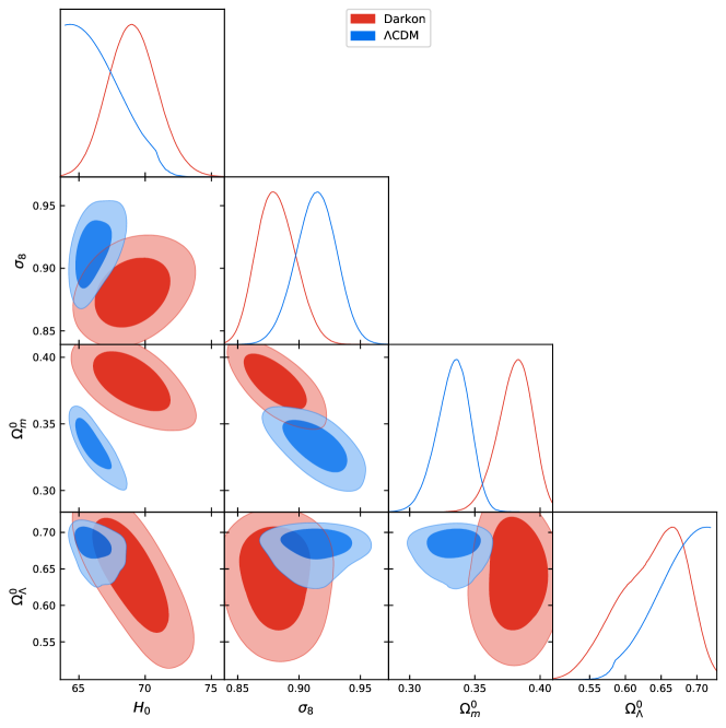
Figure 1: The corner plot of the potential (75) with the direct measurements of the Hubble expansion and the growth matter data.

Potential	$\Omega_{m}^{0}$	$H_{0}\frac{km/s}{Mpc})$	$\Omega_{\Lambda}^{0}$	$\beta$	$\sigma_{8}$	$\chi^{2}$
(75)	$0.38\pm 0.013$	$69.04_{\pm 1.75}$	$0.638_{\pm 0.04}$	$0.46_{\pm 0.03}$	$0.882_{\pm 0.178}$	84.56
Flat ($\Lambda$CDM)	$0.334_{\pm 0.012}$	$66.07_{\pm 0.877}$	$0.6796_{\pm 0.0194}$	$0$	$0.913\pm_{0.015}$	96.12

Table 1: Observational constraints and the corresponding $\chi^{2}$ for the considered cosmological models.

VI Statistical Analysis

In order to assess the viability of the model, we confront it with the observational data the solutions for Eq.(49) (the homogeneous one within the FLRW framework) and Eq.(69) (for the perturbations above the FLRW background).

We examine the following “darkon” Noether symmetry-breaking potential (with $\tilde{\phi}$ – the redefined “darkon” field (43)):

$$U(\tilde{\phi})=2M\beta^{2}\tilde{\phi}\;.$$ (75)

For the limit $\beta\rightarrow 0$ the potential goes to zero, and we recover the $\Lambda$CDM model both in the homogeneous solution as well as on the linear perturbation level.

We test the solutions that are provided by the present “darkon” model with two data sets: the direct measurements of the Hubble expansionYu et al. (2018); Moresco et al. (2018) and the growth rate data set Sagredo et al. (2018); Anagnostopoulos et al. (2019c); Basilakos and Anagnostopoulos (2020); Kazantzidis and Perivolaropoulos (2018); Gannouji et al. (2018); Kazantzidis et al. (2019); Benisty (2020).

The direct measurements of the Hubble expansion set contains $N=36$ measurements of the Hubble expansion in the redshift range $0.07\leq z\leq 2.33$. 5 measurements are based on Baryonic Acoustic Oscillations (BAOs), and the other estimated via the differential age of passive evolving galaxies. Here, the corresponding $\chi^{2}_{H}$ function reads:

$$\chi_{\mathcal{H}}^{2}={\bf\cal H}\,{\bf C}_{H,\text{cov}}^{-1}\,{\bf\cal H}^{T}\,,$$ (76)

where ${\bf\cal H}=\{H_{1}-H_{0}E(z_{1},\phi^{\nu})\,,\,...\,,\,H_{N}-H_{0}E(z_{N},\phi^{\nu})\}$ and $H_{i}$ are the observed Hubble rates at redshift $z_{i}$ ($i=1,...,N$). The matrix ${\bf C}$ denotes the covariance matrix, and $\phi^{\nu}$ denotes the other parameters on which the Hubble rate depends.

A model-independent cosmological probe, the $f\sigma_{8}$ product, is estimated from the analysis of redshift-space distortions Song and Percival (2009); Benisty (2020). There is a big number of data points. We choose to use a compilation of $f\sigma_{8}$ data that checked in terms of its robustness using information theoretical methods. The relevant chi-square function reads

$$\chi^{2}_{f\sigma 8}={f\sigma 8}\,{\bf C}_{f\sigma 8,\text{cov}}^{-1}\,{f\sigma 8}^{T}\,,$$ (77)

where $f\sigma_{8}(a_{i},\phi^{\nu+1})_{theor}=\sigma_{8}\delta^{\prime}(a_{i},\phi^{\nu})/\delta(1,\phi^{\nu})a_{i}$ and a prime denotes derivative of the scale factor $a$ with the corresponding correlation matrix. The quantity $\sigma_{8}$ is a free parameter. The statistical vector $\phi^{\nu}$ contains the other free parameters of the statistical model. The values $\delta^{\prime}(a_{i})$, $\delta(1)$ are calculated by the numerical solution of Eq. Eq.(69) for a given set of cosmological parameters.

To obtain the joint constraints on the cosmological parameters from 2 cosmological probes, we define the total $\chi^{2}_{\text{tot}}$ expression:

$$\chi_{\text{tot}}^{2}=\chi_{\mathcal{H}}^{2}+\chi^{2}_{f\sigma 8}\,.$$ (78)

Regarding the problem of data fit, we use a nested sampler as it is implemented within the open-source $Polychord$ Handley et al. (2015) with the $GetDist$ packaged Lewis (2019) to present the results. The prior we choose is with a uniform distribution, where $\Omega_{m}\in[0.2;0.4]$, $\Omega_{\Lambda}\in[0.5;0.8]$, $\sigma_{8}\in[0.5;1.2]$, $H_{0}\in[65;75]$ and $\beta\in[0;0.5]$ for the “darkon” model.

Fig. 1 presents the corner plot of the joint statistical analyses. Table 1 summarizes the joint statistics. One can see that the $\sigma_{8}$ that the potential (75) predicts is closer to the value predicted by PLANCK collaboration $\sigma_{8}=0.811\pm 0.006$ and $H_{0}=67.4\pm 0.5km/s/Mpc$. The $\chi^{2}$ per degrees of freedom for the “darkon” model yields $1.023$, while for $\Lambda$CDM the $\chi^{2}$ per degrees of freedom gives $0.899$. The fit is better when the Noether Symmetry is preserve.

VII Conclusions

This paper connects the standard $\Lambda$CDM model of cosmology to the hidden nonlinear Noether symmetry of a simple modified gravity-matter model with a single scalar field based on the formalism of non-Riemannian spacetime volume-elements. Via the Noether symmetry of its modified action the scalar field, called “darkon”, dynamically generates both cosmological constant (not present in the original action), as well as dust-like dark matter component of the pertinent stress-energy tensor – a simplest explicit realization of the $\Lambda$CDM framework. Adding Noether symmetry-breaking “darkon” potential introduces interaction (energy transfer) between dark energy and dark matter.

We calculate up to linear order of perturbations the solution for the above theory confirming that in the absence of “darkon” Noether symmetry breaking the known equation for the dark matter density contrast for the $\Lambda$CDM scenario is recovered.

We also studied the homogeneous background and linearly perturbed solutions with a specific plausible choice of “darkon” Noether symmetry-breaking potential. Using the direct measurements of the Hubble expansion and the growth matter perturbations data we find that our fit is closer to Planck data, and the $\chi^{2}/Dof$ is not significantly higher. However, to alleviate the cosmic tensions completely we should test more data sets as pantheon Type Ia supernova and measurements from the early universe as the CMB data.