Quantum simulations of a qubit of space

Abstract

In loop quantum gravity approach to Planck scale physics, quantum geometry is represented by superposition of the so-called spin network states. In the recent literature, a class of spin networks promising from the perspective of quantum simulations of quantum gravitational systems has been studied. In this case, the spin network states are represented by graphs with four-valent nodes, and two dimensional intertwiner Hilbert spaces (qubits of space) attached to them. In this article, construction of quantum circuits for a general intertwiner qubit is presented. The obtained circuits are simulated on 5-qubit (Yorktown) and 15-qubit (Melbourne) IBM superconducting quantum computers, giving satisfactory fidelities. The circuits provide building blocks for quantum simulations of complex spin networks in the future. Furthermore, a class of maximally entangled states of spin networks is introduced. As an example of application, attempts to determine transition amplitudes for a monopole and a dipole spin networks with the use of superconducting quantum processor are made.

I Introduction

In the recent articles Li:2017gvt ; Mielczarek:2018ttq ; Mielczarek:2018nnd ; Mielczarek:2018jsh ; Cohen:2020jlj ; Zhang:2020lwi an idea of performing quantum simulations of loop quantum gravity (LQG) Ashtekar:2004eh ; Rovelli:1997yv has been developed. While at present such simulations are possible to execute only for very simple systems, the approach may provide a way to investigate collective properties of Planck scale degrees of freedom in the future.

Taking into account exponential growth of the dimensionality of the Hilbert space with the increase of the involved degrees of freedom, simulation of complex quantum gravitational systems is an extremely difficult task for classical computers. On the other hand, the current progress in quantum computing technologies may open a way to simulate quantum gravitational systems unachievable to the most powerful classical supercomputers yet in this decade. Such claim is supported by the recent results of quantum computations of the sampling problem from a quasi-random quantum circuit performed on a 53 qubit quantum processor GoogleSup . Therefore, even if available quantum computing resources are still very limited, it is justified to already now prepare, test and optimize quantum circuits for the future quantum simulations of the Planck scale physics. A side benefit of such investigations is exploration of the quantum information structure of geometry, within and beyond LQG. In particular, the studies may shed a new light on such fundamental issues as emerging Gravity/Entanglement duality Ryu:2006bv ; Swingle:2009bg and related ER=EPR conjecture Susskind:2017ney . The duality has its roots in the holographic principle Susskind:1994vu and AdS/CFT correspondence Maldacena:1997re .

Following the correspondence’s holographic nature, the gravitational 3D bulk geometry is dually described by the 2D boundary. From this point of view, the LQG spin networks can be interpreted as the representations of either a state of gravity in bulk or, equivalently, the entanglement structure (similarly to tensor networks) of the boundary Han:2016xmb . In consequence, simulating quantum gravity on a quantum computer may concern either the 3D bulk or the 2D boundary. In the latter case, simulations of a quantum system at the boundary (e.g., a specific spin system) should allow reconstructing a state of quantum geometry in the bulk. It is, therefore, worth emphasizing that quantum simulations of 2D gravitational surfaces are of particular interest. The first attempt at quantum simulations in the holographic context has already been made in Ref. Li:2017qwu . Concerning LQG, an example of a relevant quantum model of a boundary has been introduced in Ref. Feller:2017ejs . The model utilizes the intertwiner degrees of freedom investigated here. Our studies may, therefore, be considered as a vestibule to quantum simulations of this and other similar models of quantum boundaries (but also the bulk geometry) in the future.

In this article, we follow the discussion presented in Mielczarek:2018jsh where a class of spin networks characterized by 4-valent nodes has been considered. It has been shown, that while spin labels at the links are given by fundamental representations of the SU(2) group, the intertwiner spaces at the nodes are two dimensional Hilbert spaces. The Hilbert spaces are invariant subspaces (singlets) of four spin-1/2 Hilbert spaces associated with holonomies, which meet at the node (see Fig. 1).

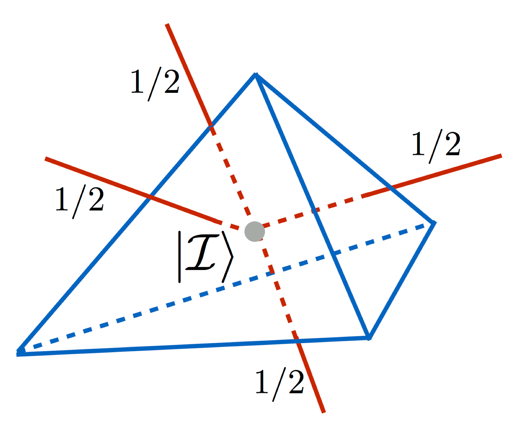
FIG. 1: 4-valent node of the spin network and its geometrical interpretation as a tetrahedon.

The singlet states are a consequence of the the local SU(2) gauge invariance imposed by the Gauss constraint in LQG, which has a form of a vector equation defining a tetrahedron (see e.g. CRFV ):

$$\sum_{i=1}^{4}\vec{J}_{i}=0,$$ (1)

where $\vec{J}_{i}$ are the angular momentum vectors normal to the faces of the tetrahedron. The components of the vector $\vec{J}_{i}=(J_{i}^{1},J_{i}^{2},J_{i}^{3})$ satisfy the $\mathfrak{su}(2)$ algebra: $\{J_{k}^{a},J_{l}^{b}\}=\delta_{kl}{\epsilon^{ab}}_{c}J_{k}^{c}$, for $a,b,c\in\{1,2,3\}$. The $\vec{J}_{i}$ vectors are associated to the areas $A_{i}:=8\pi l^{2}_{\text{Pl}}\gamma\sqrt{\vec{J}_{i}\cdot\vec{J}_{i}}$ of the faces, where $l_{\text{Pl}}:=\sqrt{G}\approx 1.62\cdot 10^{-35}$ m is the Planck length, $G$ is the Newton’s constant and $\hslash=1=c$. Here, $\gamma$ is the Barbero-Immirzi parameter Immirzi:1996dr ; Barbero:1994ap , which plays an important role in LQG.

In such a case, a general intertwiner state - an intertwiner qubit - can be written as Mielczarek:2018jsh :

$$|\mathcal{I}\rangle=\cos(\theta/2)|0_{s}\rangle+e^{i\phi}\sin(\theta/2)|1_{s}\rangle,$$ (2)

where $\theta\in[0,\pi]$ and $\phi\in[0,2\pi)$ are angles on the Bloch sphere. The $|0_{s}\rangle$ and $|1_{s}\rangle$ are basis states, corresponding to two linearly independent singlets of four spin-1/2 DOFs (qubits) in the $s$-channel Feller:2015yta :

$$|0_{s}\rangle =|S\rangle|S\rangle,$$ (3)

$$|1_{s}\rangle =\frac{1}{\sqrt{3}}\left(|T_{+}\rangle|T_{-}\rangle+|T_{-}\rangle|T_{+}\rangle-|T_{0}\rangle|T_{0}\rangle\right),$$ (4)

where

$$|S\rangle =\frac{1}{\sqrt{2}}\left(|01\rangle-|10\rangle\right),$$ (5)

$$|T_{+}\rangle =|00\rangle,$$ (6)

$$|T_{0}\rangle =\frac{1}{\sqrt{2}}\left(|01\rangle+|10\rangle\right),$$ (7)

$$|T_{-}\rangle =|11\rangle,$$ (8)

are two spin-1/2 singlet and triplet states respectively. The Hilbert space of the spin-1/2 DOF is $\mathcal{H}_{1/2}=\text{span}\{|0\rangle,|1\rangle\}$.

Physically, the intertwiner space is associated with the quantum of volume Rovelli:1994ge ; Ashtekar:1997fb . This can be shown by considering volume operator $\hat{V}$ in LQG, defined as follows CRFV :

$$\hat{V}:=\frac{\sqrt{2}}{3}l_{\text{Pl}}^{3}(8\pi\gamma)^{\frac{3}{2}}\sqrt{\left|\hat{\vec{J}}_{1}\cdot(\hat{\vec{J}}_{2}\times\hat{\vec{J}}_{3})\right|},$$ (9)

where $\hat{\vec{J}}_{i}$ are the angular momentum vector operators. The volume operator is defined as a positive-definite function of the triple product $\vec{J}_{1}\cdot(\vec{J}_{2}\times\vec{J}_{3})$, the sign of which depends on the orientation of space. The two possible signs discriminate between the two eigenvalues of the operator $\hat{\vec{J}}_{1}\cdot(\hat{\vec{J}}_{2}\times\hat{\vec{J}}_{3})$. In order to keep this information at the level of the volume positive-definite operator $\hat{V}$, one can extend its definition (9) to the oriented volume case. In consequence, the two signs will distinguish the two (initially degenerated) eigenvalues of the volume operator. One can find that, the following superpositions of the basis states $|0_{s}\rangle$ and $|1_{s}\rangle$:

$$|V_{+}\rangle = \frac{1}{\sqrt{2}}\left(|0_{s}\rangle-i|1_{s}\rangle\right),$$ (10)

$$|V_{-}\rangle = \frac{1}{\sqrt{2}}\left(|0_{s}\rangle+i|1_{s}\rangle\right),$$ (11)

are eigenstates of the volume operator, such that the oriented eigenvalues satisfy: $\hat{V}|V_{+}\rangle=+V_{0}|V_{+}\rangle$ and $\hat{V}|V_{-}\rangle=-V_{0}|V_{-}\rangle$ CRFV . The $V_{0}:=\frac{l^{3}_{\text{Pl}}(8\pi\gamma)^{\frac{3}{2}}}{\sqrt{6\sqrt{3}}}$ is a quantum of 3-volume in LQG. This justifies why we call the two dimensional intertwiner a qubit of space.

Worth mentioning is that the intertwiner states are relevant in quantum information theory. Namely, encoding one logical qubit (the intertwiner qubit) in four physical qubits allows for quantum communication without a shared reference frame Bartlett . Let $\rho_{A}$ be a state (i.e. density matrix) that Alice wants to send to Bob. Bob because of his lack of knowledge about Alice’s reference frame receives state $\rho_{B}$:

$$\rho_{B}=\int_{G}dgU\left(g\right)\rho_{A}U^{\dagger}\left(g\right),$$ (12)

where $g\in G$ and $G$ is a group of transformations between the two reference frames, and $dg$ is the Haar measure. The operation $U\left(g\right):=U_{1}\left(g\right)\otimes U_{2}\left(g\right)\otimes U_{3}\left(g\right)\otimes U_{4}\left(g\right)$ is a tensor product of (the same) single-qubit unitary operators $U_{i}(g)$ for $i=1,2,3,4$, acting on the four composite qubits of the intertwiner states. In the case when Alice and Bob share no knowledge about the orientation of their frames, we have $G=SU\left(2\right)$. Consequently, one finds that in order to have $\rho_{A}=\rho_{B}$, the states invariant under the action of this group must be considered. The is satisfied by the intertwiner qubits considered here. Further discussion of this property in the quantum gravitational context can be found in Ref. Livine:2005mw .

In Ref. Mielczarek:2018jsh a quantum circuit for the $|0_{s}\rangle$ basis state has been investigated and simulated on the IBM Q 5-qubit quantum processor. In this article, the analysis is extended to the general intertwiner qubit $|\mathcal{I}\rangle$ given by Eq. 2. In Sec. II a quantum circuit for a general intertwiner state is introduced. Then, in Sec. III the circuit is transpilated such that it fits to the topologies of the superconducting IBM quantum processors. The Sec. IV presents reduced forms of the quantum circuits for the special cases of the basis states: $|0_{s}\rangle$ and $|1_{s}\rangle$. In Sec. V six representative states of the intertwiner qubit are simulated on IBM 5 and 15 qubit quantum processors, which are available for cloud computing. Then, in Sec. VI a general discussion of the transition amplitudes between the spin network states is given. A class of maximally entangled states which introduce quantum correlations between intertwiner qubits is introduced in Sec. VII. The maximally entangled states are applied to the special cases of the monopole (Sec.VIII) and dipole (Sec. IX) spin networks, for which attempts to determine transition amplitudes with the use of superconducting IBM quantum processors are made. Our results are summarized in Sec. X. The article is accomplished with two appendices. Appendix A contains numerical results obtained from simulations of the interwiner qubits states, discussed in Sec. V. In Appendix B, results of test performed on the 15-qubit IBM quantum computer Melbourne are shown.

II Quantum circuit

The purpose of this section is to find quantum circuit representation of the unitary operator $\hat{U}_{\mathcal{I}}$, such that:

$$|\mathcal{I}\rangle=\hat{U}_{\mathcal{I}}|0000\rangle.$$ (13)

Here, the $|\mathcal{I}\rangle$ is a general intertwiner qubit state $|\mathcal{I}\rangle\in\mathcal{H}_{\mathcal{I}}:=\text{span}\{|0_{s}\rangle,|1_{s}\rangle\}$, given by Eq. 2 and $|0000\rangle$ is the initial state of the quantum register.

The $\hat{U}_{\mathcal{I}}$ is a state preparation operator. The procedure of preparing $|\mathcal{I}\rangle$ is, however, not unique since there are infinitely many operators $\hat{U}_{\mathcal{I}}$ that satisfy Eq. 13. This is because only first column in the matrix representation of $\hat{U}_{\mathcal{I}}$ is fixed and there are still $n^{2}-2n-1=223$ undetermined free real parameters (here $n=\text{dim}\otimes\mathcal{H}_{1/2}^{4}=16$ and the total irrelevant phase has also been subtracted). Furthermore, in general, expressing an operator in terms of quantum gates is a difficult task. Here, the goal is achieved by utilising some properties of the state $|\mathcal{I}\rangle$, which allows for systematic expressing of the state in terms of the elementary quantum gates acting on the initial state $|0000\rangle$.

Worth mentioning at this point is that, in general, one could expect that some ancilla qubits may also be involved. However, as we will show here, additional logical qubits are not required to produce the state $|\mathcal{I}\rangle$. However, while noisy physical qubits are considered, quantum error correction codes need to be involved, which unavoidably utilize additional physical qubits. In this article, we will restrict our considerations to the level of logical qubits and the quantum error correction codes will not be discussed.

In order to find the quantum circuit representing the operator $\hat{U}_{\mathcal{I}}$ let us first apply Eqs. 3 and 4 to Eq. 2, which leads to:

$$|\mathcal{I}\rangle =\frac{c_{1}}{\sqrt{2}}(|0011\rangle+|1100\rangle)$$

$$+\frac{c_{2}}{\sqrt{2}}(|0101\rangle+|1010\rangle)$$

$$+\frac{c_{3}}{\sqrt{2}}(|0110\rangle+|1001\rangle),$$ (14)

where coefficients $c_{1}$, $c_{2}$ and $c_{3}$ are complex-valued coefficients expressed as follows:

$$c_{1} =\sqrt{\frac{2}{3}}e^{i\phi}\sin(\theta/2),$$ (15)

$$c_{2} =\frac{1}{\sqrt{2}}\left(\cos(\theta/2)-\frac{1}{\sqrt{3}}e^{i\phi}\sin(\theta/2)\right)$$

$$=\frac{e^{i\chi_{+}}}{\sqrt{2}}\sqrt{1-\frac{2}{3}\sin^{2}(\theta/2)-\frac{\sin\theta\cos\phi}{\sqrt{3}}},$$ (16)

$$c_{3} =\frac{1}{\sqrt{2}}\left(-\cos(\theta/2)-\frac{1}{\sqrt{3}}e^{i\phi}\sin(\theta/2)\right)$$

$$=\frac{e^{i\chi_{-}}}{\sqrt{2}}\sqrt{1-\frac{2}{3}\sin^{2}(\theta/2)+\frac{\sin\theta\cos\phi}{\sqrt{3}}},$$ (17)

together with the phases

$$\chi_{\pm}= \arctan\left(\frac{\sin(\phi)\tan(\theta/2)}{\mp\sqrt{3}+\cos(\phi)\tan(\theta/2)}\right)$$

$$+ \frac{\pi}{2}\left[1-\text{sgn}\left(\pm\cos\left(\frac{\theta}{2}\right)-\frac{\cos\phi\sin\left(\frac{\theta}{2}\right)}{\sqrt{3}}\right)\right].$$ (18)

The coefficients (15), (16) and (17) satisfy the two conditions:

$$\sum_{i=1}^{3}|c_{i}|^{2}=1,\ \text{and}\ \ \sum_{i=1}^{3}c_{i}=0.$$ (19)

Let us observe that the states in the pairs in Eq. 14 are mutually negated. Furthermore, in each pair, the states have the same first binary digit. This suggests to consider an operator $\hat{N}$, which acts as follows:

$$\hat{N}|0b_{1}b_{2}b_{3}\rangle=\frac{\left(|0b_{1}b_{2}b_{3}\rangle+|1\bar{b}_{1}\bar{b}_{2}\bar{b}_{3}\rangle\right)}{\sqrt{2}},$$ (20)

generating from a given state $|0b_{1}b_{2}b_{3}\rangle$ an equally weighted superposition of the state and its negation. The $b_{1},b_{2},b_{3}\in\{0,1\}$. Quantum circuit corresponding to the action of $\hat{N}$ can be constructed using combination of a single Hadamard gate and three CNOT gates. The quantum circuit is shown in Fig. 2.

FIG. 2: Quantum circuit for the operator $\hat{N}$.

Employing the operator $\hat{N}$, the state $|\mathcal{I}\rangle$ can be expressed as,

$$|\mathcal{I}\rangle=\hat{N}(|0\rangle|\psi\rangle)$$ (21)

where $|\psi\rangle$ is a 3-qubit state:

$$|\psi\rangle=c_{1}|011\rangle+c_{2}|101\rangle+c_{3}|110\rangle.$$ (22)

The task is now to find an operator $\hat{M}$, action o which is:

$$|\psi\rangle=\hat{M}|000\rangle.$$ (23)

One can find that the operator $\hat{M}$ is represented by the circuit presented in Fig. 3.

FIG. 3: Quantum circuit for the operator $\hat{M}$.

In the circuit, the unitary operation $\hat{U}$, given by the special unitary matrix:

$$U=\left(\begin{array}[]{cc}c_{1}&\sqrt{|c_{2}|^{2}+|c_{3}|^{2}}\\ -\sqrt{|c_{2}|^{2}+|c_{3}|^{2}}&c_{1}^{*}\end{array}\right),$$ (24)

is performed first on the top qubit. Then, controlled-V 2-qubit gate is performed, where the special unitary matrix V is given by:

$$V=\left(\begin{array}[]{cc}-\frac{c_{2}}{\sqrt{|c_{2}|^{2}+|c_{3}|^{2}}}&\frac{c_{3}^{*}}{\sqrt{|c_{2}|^{2}+|c_{3}|^{2}}}\\ -\frac{c_{3}}{\sqrt{|c_{2}|^{2}+|c_{3}|^{2}}}&-\frac{c_{2}^{*}}{\sqrt{|c_{2}|^{2}+|c_{3}|^{2}}}\end{array}\right).$$ (25)

Finally, a sequence of three anti-CNOT gates, which allow to obtain deserved sequences of bits, are applied.

Combining action of the operators $\hat{M}$ and $\hat{N}$ the general intertwiner state (2) can now be written as:

$$|\mathcal{I}\rangle=\hat{U}_{\mathcal{I}}|0000\rangle=\hat{N}(\hat{\mathbb{I}}\otimes\hat{M})|0000\rangle.$$ (26)

The corresponding quantum circuit is shown in Fig. 4.

FIG. 4: A quantum circuit corresponding to the operator $\hat{U}_{\mathcal{I}}$.

III Transpilation

Physical realizations of quantum computers impose restrictions on the types of quantum circuits which can be executed or implemented directly on a given quantum processor. In particular, the limitation is due to topology of couplings between the physical qubits. Because of this, transpilation of the considered quantum circuit has to be performed, such that the circuit can be simulated on a given hardware.

Here, we will consider transpilation of the quantum circuit shown in Fig. 4 to the form compatible with the 5-qubit and 15-qubit quantum processors, made available by IBM via cloud computing platform IBM .

The transpilation concerns not only connectivity of the quantum processor but also the types of gates which are possible to execute. The Hadamard and CNOT gates are part of the standard IBM library. The anti-CNOT gate can be built utilizing the CNOT gate and two bit-flip $\hat{X}$ gates (corresponding to the Pauli matrix $X=\left(\begin{array}[]{cc}0&1\\ 1&0\end{array}\right)$): $(\hat{X}\otimes\hat{I})\widehat{\text{CNOT}}(\hat{X}\otimes\hat{I})$. Furthermore, IBM utilizes the following gates:

$$U_{1}\left(\rho\right)=\left(\begin{array}[]{cc}1&0\\ 0&e^{i\rho}\end{array}\right),$$ (27)

and

$$U_{3}\left(\theta,\phi,\lambda\right)=\left(\begin{array}[]{cc}\cos\left(\theta/2\right)&-e^{i\lambda}\sin\left(\theta/2\right)\\ e^{i\phi}\sin\left(\theta/2\right)&e^{i\lambda+i\phi}\cos\left(\theta/2\right),\end{array}\right),$$ (28)

which can be used to construct the operators $\hat{U}$ and $\hat{V}$. Namely, the operator $\hat{U}$ can be expressed as:

$$U=U_{3}\left(\theta_{U},\phi_{U},\lambda_{U}\right)X$$ (29)

where the angles are

$$\theta_{U} =2\arcsin\left(\sqrt{\frac{2}{3}}\sin\left(\theta/2\right)\right),$$ (30)

$$\phi_{U} =-\phi,$$ (31)

$$\lambda_{U} =\pi+\phi.$$ (32)

Similarly, the operator $\hat{V}$ can be written as:

$$V=U_{3}\left(\theta_{V},\phi_{V},\lambda_{V}\right)XU_{1}\left(\rho_{V}\right),$$ (33)

where

$$\theta_{V} =2\arcsin\left(\sqrt{\frac{1}{2}+\frac{\sin\theta\cos\phi}{2\sqrt{3}\left(1-2/3\sin^{2}\theta\right)}}\right),$$ (34)

$$\phi_{V} =-\pi+\chi_{+}-\chi_{-},$$ (35)

$$\lambda_{V} =\chi_{-},$$ (36)

$$\rho_{V} =\pi-\chi_{+}.$$ (37)

Let us now proceed to the topological considerations. In Fig. 5, connectivity of the 5-qubit IBM quantum processor is shown.

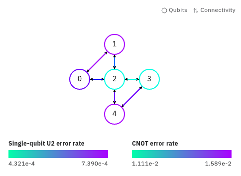
FIG. 5: Connectivity of the IBM Q 5-qubit quantum processor (Yorktown). Obtained from IBM quantum cloud computing service IBM .

The transpilated version of the circuit (4) in agreement with the topology of the 5-qubit quantum processor (Yorktown) is presented in Fig. 6.

FIG. 6: A quantum circuit corresponding to the operator $\hat{U}_{\mathcal{I}}$, compatible with the the 5-qubit IBM quantum processor Yorktown.

In Fig. 7 connectivity of the 15-qubit IBM quantum processor is shown.

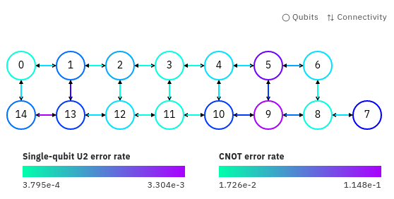
FIG. 7: Connectivity of the IBM Q 15-qubit quantum processor (Melbourne). Obtained from IBM quantum cloud computing service IBM .

Two alternative versions of the transpilated circuit (4), being in agreement with the topology of the 15-qubit quantum processor (Melbourne), are presented in Fig. 8 and Fig. 9.

FIG. 8: A quantum circuit corresponding to the operator $\hat{U}_{\mathcal{I}}$, compatible with the the 15-qubit IBM quantum processor Melbourne - version 1.

FIG. 9: A quantum circuit corresponding to the operator $\hat{U}_{\mathcal{I}}$, compatible with the the 15-qubit IBM quantum processor Melbourne - version 2.

One final issue is the controlled-V gate, which not necessary can be directly implemented. In that case, the 2-qubit gate can be expressed with the use of standard decomposition presented in Fig. 10, for a unitary operator $\hat{W}$ Barenco .

FIG. 10: Control-W gate and its equivalent expressed with the use of single qubit gates and CNOT gates.

Here, $\hat{W}=\hat{V}\hat{S}$, where $\hat{V}$ is a special unitary operator and $\hat{S}=e^{i\delta}\hat{\mathbb{I}}$, with the phase $\delta\in\mathbb{R}$. The $E$ gate is given by the matrix $E=\left(\begin{array}[]{cc}1&0\\ 0&e^{i\delta}\\ \end{array}\right)$. Furthermore, the involved gates $\hat{A}$, $\hat{B}$ and $\hat{C}$ are 1-qubit gates, satisfying conditions $\hat{C}\hat{B}\hat{A}=\hat{\mathbb{I}}$ and $\hat{C}\hat{X}\hat{B}\hat{X}\hat{A}=\hat{V}$. In our case, because $V$ given by Eq. 25 is a special unitary matrix, we have $\delta=0$ so $\hat{W}=\hat{V}$ and matrix representations of the gates $A$, $B$ and $C$ are:

$$A=\left(\begin{array}[]{cc}\cos\left(\frac{\rho}{4}\right)&\sin\left(\frac{\rho}{4}\right)\\ e^{i(\chi_{-}-\chi_{+})}\sin\left(\frac{\rho}{4}\right)&-e^{i(\chi_{-}-\chi_{+})}\cos\left(\frac{\rho}{4}\right)\\ \end{array}\right),$$ (40)

$$B=\left(\begin{array}[]{cc}\cos\left(\frac{\rho}{4}\right)&e^{i\chi_{+}}\sin\left(\frac{\rho}{4}\right)\\ \sin\left(\frac{\rho}{4}\right)&-e^{i\chi_{+}}\cos\left(\frac{\rho}{4}\right)\\ \end{array}\right),$$ (43)

$$C=\left(\begin{array}[]{cc}1&0\\ 0&e^{-i\chi_{-}}\\ \end{array}\right),$$ (46)

where

$$\rho=2\arccos\left(\sqrt{\frac{1}{2}\left(1-\frac{\sin\theta\cos\phi}{\sqrt{3}\left(1-\frac{2}{3}\sin^{2}\left(\frac{\theta}{2}\right)\right)}\right)}\right).$$ (47)

Furthermore, the gates can be constructed with use of the $U_{3}$ and $U_{1}$ gates as follows:

$$A=U_{3}\left(\frac{\rho}{2},\chi_{-}-\chi_{+},\pi\right),$$ (48)

$$B=U_{3}\left(\frac{\rho}{2},0,\chi_{+}+\pi\right),$$ (49)

$$C=U_{1}\left(-\chi_{-}\right).$$ (50)

IV Exemplary states

In this section we will simplify the obtained general quantum circuit shown in Fig. 4 for the special cases of the intertwiner qubit basis states: $|0_{s}\rangle$ and $|1_{s}\rangle$. This will allow to slightly reduce the general circuit, which is relevant from the perspective of quantum simulation, where the number of involved gates has to be minimized because of the issue of errors.

IV.1 The state $|0_{s}\rangle$

The quantum circuit for the $|0_{s}\rangle$ state has already been a subject of investigation in Ref. Mielczarek:2018jsh and is shown in Fig. 11.

FIG. 11: Quantum circuit for the $|0_{s}\rangle$ state discussed in Ref. Mielczarek:2018jsh .

Here, we will present an alternative construction of the state, starting from the general circuit shown in Fig. 4. Taking $\theta=0$, we find that the coefficients:

$$c_{1}=0,\ \ c_{2}=\frac{1}{\sqrt{2}},\ \ c_{3}=-\frac{1}{\sqrt{2}}.$$ (51)

In consequence, the $\hat{U}$ and $\hat{V}$ operators (see Eqs. 24 and 25) are now represented by the following matrices:

$$U=\left(\begin{array}[]{cc}0&1\\ -1&0\end{array}\right)$$ (52)

and

$$V=\frac{1}{\sqrt{2}}\left(\begin{array}[]{cc}-1&-1\\ 1&-1\end{array}\right).$$ (53)

This allows to reduce the circuit from Fig. 4 to the one presented in Fig. 12.

FIG. 12: Quantum circuit for the $|0_{s}\rangle$ state.

IV.2 The state $|1_{s}\rangle$

For the state $|1_{s}\rangle$, we take $\theta=\pi$, which reduces the coefficients (15), (16) and (17) to:

$$c_{1}=\sqrt{\frac{2}{3}},\ \ c_{2}=-\frac{1}{\sqrt{6}},\ \ c_{3}=-\frac{1}{\sqrt{6}},$$ (54)

such that the $U$ and $V$ matrices are

$$U=\sqrt{\frac{2}{3}}\left(\begin{array}[]{cc}1&\frac{1}{\sqrt{2}}\\ -\frac{1}{\sqrt{2}}&1\end{array}\right),$$ (55)

and

$$V=\frac{1}{\sqrt{2}}\left(\begin{array}[]{cc}1&-1\\ 1&1\end{array}\right).$$ (56)

This allows to reduce the circuit from Fig. 4 to the one presented in Fig. 13.

FIG. 13: Quantum circuit for the $|1_{s}\rangle$ state.

V Quantum simulations

The quantum circuits for a single intertwiner qubit introduced in the previous sections represent unitary operators acting in 16 dimensional Hilbert space, being a tensor product of four $\mathcal{H}_{1/2}$ Hilbert spaces. Such a case is easy to handle wit the use of classical computer. However, the difficulty came when more complex systems are considered. In our case, four qubits are needed to define a single intertwiner qubit. Therefore, a spin network with $N$ four-valent nodes requires $4N$ logical qubits. The corresponding Hilbert space has dimension $\text{dim}\otimes_{i=1}^{4N}\mathcal{H}_{i}=2^{4N}$. In case of a general quantum circuit, classical simulations of the systems with $N\sim 20$ ($\sim 80$ logical qubits) is already beyond the reach of any currently existing classical supercomputer Chen . On the other hand, (noisy) quantum computers with the number of qubits $\sim 50$ already exist and the ones with $\sim 100$ are under development (see e.g. IBM ; Google ; Rigetti ; Ionq ). This prognosis that simulations of spin networks with $N\sim 20$ and more will become feasible in the coming years (see also discussion in Ref. Mielczarek:2018jsh ). However, as we will already see while considering 15 qubit quantum chip, the issue of errors reduction remains to be a challange even in processors with over a dozen of qubits. Furthermore, we have to emphasize that the superconducting quantum computers are characterized by relatively short coherence times, which limits depth of the quantum circuits which can be simulated successfully.

Here, we will present results of simulations of exemplary states of the intertwiner qubit performed on 5-qubit (Yorktown) and 15-qubit (Melbourne) IBM superconducting quantum processors, topologies of which are shown in Fig. 5 and Fig. 7 respectively. In the figures, errors of the particular qubits at the time of simulations are also presented.

The six representative states which are considered are: $|0_{s}\rangle$, $|1_{s}\rangle$, $|+\rangle:=\frac{|0_{s}\rangle+|1_{s}\rangle}{\sqrt{2}}$, $|-\rangle:=\frac{|0_{s}\rangle-|1_{s}\rangle}{\sqrt{2}}$, $|\leftturn\rangle:=\frac{|0_{s}\rangle-i|1_{s}\rangle}{\sqrt{2}}$ and $|\rightturn\rangle:=\frac{|0_{s}\rangle+i|1_{s}\rangle}{\sqrt{2}}$. The $|0_{s}\rangle$ and $|1_{s}\rangle$ states correspond to the points on the north and south pole of the Bloch sphere correspondingly. The remaining four states are the points located at the equator of Bloch sphere, and are evenly distributed with the polar angle difference $\Delta\phi=\frac{\pi}{2}$. The considered states have direct physical interpretation if they are referred to light. Namely, if $|0_{s}\rangle$, $|1_{s}\rangle$ are horizontal $(|\text{H}\rangle)$ and vertical $(|\text{V}\rangle)$ linear polarization states of a photon respectively, then the $|+\rangle$ and $|-\rangle$ are $\pm\frac{\pi}{4}$ linear polarization states. The $|\leftturn\rangle$ is a left-hand circular polarization state and $|\rightturn\rangle$ is a right-hand circular polarization state, which justifies the applied notation. Furthermore, the $|\leftturn\rangle$ and $|\rightturn\rangle$ are also eigenstates of the volume operator. Namely, based on (10) and (11) one can see that:

$$|\leftturn\rangle=|V_{+}\rangle\ \text{and}\ \ |\rightturn\rangle=|V_{-}\rangle.$$ (57)

In the simulations, a sequence of 10 computational rounds each containing 1024 shots was performed for every of the investigated states. The simulations were performed on both the 5-qubit Yorktown quantum processor and 15-qubit Melbourne quantum processor. Topologies of the processors together with the errors (single-qubit and CNOT 2-qubit gate) at the time of simulations are depicted in Fig. 5 and Fig. 7. The obtained averaged measured probabilities of the basis states for each of the states are shown in Fig. 14. Detailed numerical results of the simulations can be found in Appendix A.

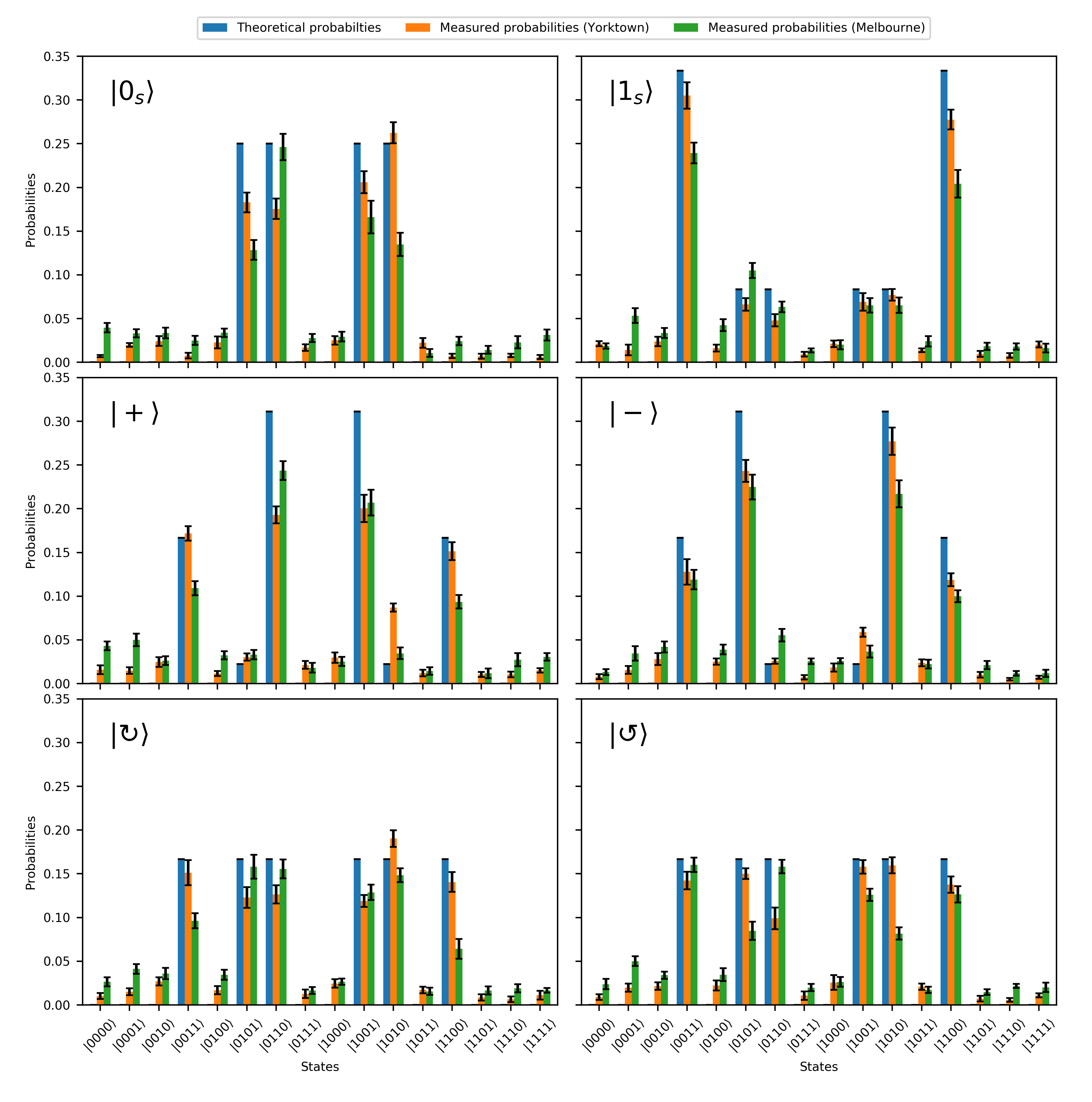
FIG. 14: Measured and theoretical probabilities for the six representative states.

In order to quantify difference between the measured states and theoretical values we use the classical fidelity function (Bhattacharyya distance):

$$F\left(p,q\right)=\sum_{i}\sqrt{p_{i}q_{i}}.$$ (58)

More detailed analysis would require quantum tomography of the states. However, consideration of the classical fidelity function is sufficient for our purpose. The obtained fidelities are collected in Table 1, and presented in Fig. 15.

$$\begin{array}[]{|c|c|c|}\hline\cr\text{State}&\text{Yorktown}&\text{Melbourne}\\ \hline\cr|0_{s}\rangle&0.906\pm 0.005&0.814\pm 0.009\\ |1_{s}\rangle&0.916\pm 0.007&0.856\pm 0.008\\ |+\rangle&0.892\pm 0.007&0.843\pm 0.006\\ |-\rangle&0.915\pm 0.007&0.857\pm 0.007\\ |\circlearrowright\rangle&0.918\pm 0.008&0.856\pm 0.008\\ |\circlearrowleft\rangle&0.917\pm 0.008&0.851\pm 0.007\\ \hline\cr\end{array}$$

Table 1: Values of fidelity for the six representative states under consideration.

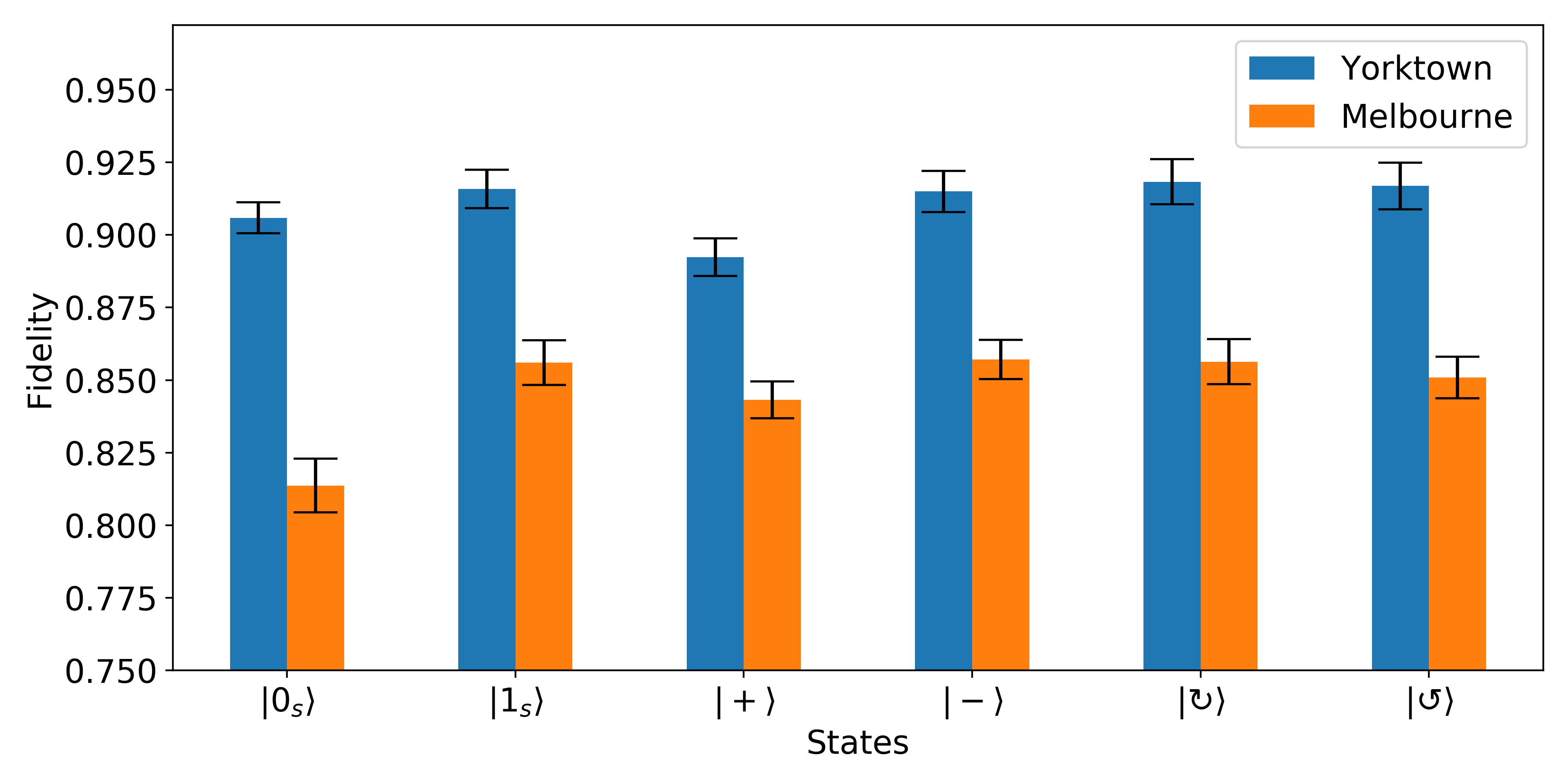
FIG. 15: Fidelity for the six representative states of the intertwiner qubit generated on 5-qubit (Yorktown) and 15-qubit (Melbourne) IBM quantum computers.

In case of the 5-qubit chip, the fidelities of the obtained states reach the level of $F\approx 90$ %. This is a significant increase comparing to the fidelity $F\approx 71$ % of the state $|0_{s}\rangle$ obtained in Ref. Mielczarek:2018jsh . Furthermore, simulations of the same states performed on the 15-qubit chip are at the level $F\approx 85$ %. There is no significant difference in the fidelities depending on which state is considered.

For comparison, the fidelities obtained in Ref. Li:2017gvt (employing molecular quantum computer) are better than those obtained here. However, in our approach the superconducting chip was used, which despite of being more noisy, gives better perspective for scaling to more complicated cases. On the other hand, in Ref. Zhang:2020lwi spin foam vertex amplitude (composed of five intertwiner qubits) has been simulated with fidelity $0.832\pm 0.005$, which is lower than almost all of the fidelities obtained here. This state had, however, more complex circuit structure than the circuits considered here. Furthermore, the results were possible to obtain because the simulations were performed directly on the intertwiner qubits.

The states’ imperfectness is mostly because of the errors associated with three factors: preparation of the initial state, implementation of the quantum gates, and readout. The errors (mainly corresponding to the two-qubit gates) have been significantly reduced over recent years. The errors of gates are shown in Fig.5 and in Fig.7.

In particular, in case of the Yorktown processor, the error of the single-qubit $U_{2}\left(\lambda,\phi\right)=\frac{1}{\sqrt{2}}\left(\begin{array}[]{cc}1&-e^{i\lambda}\\ e^{i\phi}&e^{i\left(\phi+\lambda\right)}\end{array}\right)$ gate is in range between $4.3\cdot 10^{-4}$ and $7.4\cdot 10^{-4}$. For the CNOT gate the error rate is between $1.1\cdot 10^{-2}$ and $1.6\cdot 10^{-2}$. For the Melbourne processor these errors are between $3.8\cdot 10^{-4}$ and $3.3\cdot 10^{-3}$ and between $1.7\cdot 10^{-2}$ and $1.1\cdot 10^{-1}$ respectively. The single-qubit $U_{2}$ error rates and CNOT error rates have been measured using randomized benchmarking procedure benchmarking . Despite of the considerable hardware improvement, quantum error corrections codes Lidar can also be implemented to further reduce the errors. However, this can be achieved only in a quantum chip with a sufficiently high number of physical qubits. This does not concern the currently available solutions. However, a set of methods called error mitigation mitigation can also be used to further improve the results. We plan to apply these methods in our future research.

VI Transition amplitudes

The results presented so far can be applied to evaluate transition amplitudes between states of spin networks (of fixed topology), representing different quantum geometries. In case of quantum gravity, and other quantum constrained systems, the subtlety is that the states under consideration have to be appropriately projected onto the physical Hilbert space $\mathcal{H}_{\text{phys}}$. In consequence, while some kinematical states $|\psi_{1}\rangle,|\psi_{2}\rangle\in\mathcal{H}_{\text{kin}}$ are considered, the corresponding transition amplitude has the following form:

$$A\left(\psi_{1},\psi_{2}\right):=\langle\psi_{2}|\hat{P}|\psi_{1}\rangle,$$ (59)

where $\hat{P}$ is a non-unitary, but Hermitian ($\hat{P}^{\dagger}=\hat{P}$) and idempotent ($\hat{P}^{2}=\hat{P}$), projector operator. In consequence, the $\hat{P}$ cannot be associated with a unitary quantum circuit. On the other hand, in the context of quantum computing, action of the projection operators is associated with quantum measurements.

In case when more than one constraint is involved, as in the case of gravity, the projection operator is a composition of projection operators for the individual constraints:

$$\hat{P}=\hat{P}_{1}\circ\hat{P}_{2}\circ\dots\circ\hat{P}_{m},$$ (60)

where $m$ is the number of constraints.

In LQG, the constraint are grouped into the three types: Gauss constraint, Diffeomeorphism constraint (vector constraint) and the Hamiltonian constraint (scalar constraint). Here, we will focus our attention on the case of the Gauss constraint, which is employed in the construction of the spin network spates. The vector constraint is on the other hand satisfied just by the graph structure of the spin network, so it is satisfied by construction. The scalar constraint is the most difficult to satisfy and we are not going to discuss it here. However, quantum computing methods provide some new possibilities to address the problem Mielczarek:2018ttq .

In order to compute the amplitude (59) with the use of quantum circuits, let us consider operators $\hat{U}_{\psi_{1}}$ and $\hat{U}_{\psi_{2}}$, defined such that $|\psi_{1}\rangle=\hat{U}_{\psi_{1}}|{\bf 0}\rangle$ and $|\psi_{2}\rangle=\hat{U}_{\psi_{2}}|{\bf 0}\rangle$. The $|{\bf 0}\rangle$ is an initial state of the quantum register, which in case of the spin network with $N$ four-valent nodes is $|{\bf 0}\rangle=\otimes_{i=1}^{4N}|0\rangle$. In consequence, the transition amplitude (59) takes the form:

$$\langle\psi_{2}|\hat{P}|\psi_{1}\rangle=\langle{\bf 0}|\hat{U}^{\dagger}_{\psi_{2}}\hat{P}\hat{U}_{\psi_{1}}|{\bf 0}\rangle.$$ (61)

Because $\hat{P}$ is a non-unitary operator, the operator $\hat{U}^{\dagger}_{\psi_{2}}\hat{P}\hat{U}_{\psi_{1}}$ cannot be represented by a standard quantum circuit. There is, however, a special case when at least one of the states $|\psi_{1}\rangle$ and $|\psi_{2}\rangle$ is invariant under the action of the projection operator $\hat{P}$. Then, for the Gauss constraint, this means that at least one of the states is a superposition of spin network states.

Let us examine such possibility first for the case of a single node of a spin network. In that case, for the intertwiner qubit, the projection operator associated with the Gauss constraint takes the form:

$$\hat{P}_{\text{G}}=|0_{s}\rangle\langle 0_{s}|+|1_{s}\rangle\langle 1_{s}|.$$ (62)

Then, if e.g. $|\psi_{1}\rangle$ is a state of intertwiner qubit, it can be expressed as follows:

$$|\psi_{1}\rangle=\hat{U}_{\psi_{1}}|{\bf 0}\rangle=\cos(\theta_{1}/2)|0_{s}\rangle+e^{i\phi_{1}}\sin(\theta_{1}/2)|1_{s}\rangle,$$ (63)

where now $|{\bf 0}\rangle=|0000\rangle$. It is straightforward to show that $\hat{P}_{\text{G}}|\psi_{1}\rangle=|\psi_{1}\rangle$ and, in consequence, in the considered case, the transition amplitude (61) reduces to

$$\langle\psi_{2}|\hat{P}_{\text{G}}|\psi_{1}\rangle=\langle{\bf 0}|\hat{U}^{\dagger}_{\psi_{2}}\hat{U}_{\psi_{1}}|{\bf 0}\rangle.$$ (64)

Therefore, unitary operator $\hat{U}:=\hat{U}^{\dagger}_{\psi_{2}}\hat{U}_{\psi_{1}}$ can be introduced, which can be associated with a quantum circuit. For transition between two intertwiner qubit states, the $|\psi_{1}\rangle=|\mathcal{I}\rangle$ and $|\psi_{2}\rangle=|\mathcal{I}^{\prime}\rangle$, the quantum circuit corresponding to the operator $\hat{U}=\hat{U}^{\dagger}_{\psi_{2}}\hat{U}_{\psi_{1}}$ is shown in Fig. 16.

FIG. 16: Quantum circuit for the transition amplitude operator $\hat{U}=\hat{U}^{\dagger}_{\mathcal{I}^{\prime}}\hat{U}_{\mathcal{I}}$ between two arbitrary intertwiner states $|\mathcal{I}\rangle$ and $|\mathcal{I}^{\prime}\rangle$.

The $U$ and $V$ are matrices associated with the state $|\mathcal{I}\rangle$ and $U^{\prime}$ and $V^{\prime}$ are associated with $|\mathcal{I^{\prime}}\rangle$, in accordance to the circuit presented in Fig. 4.

Using the fact that $\hat{X}$, $\hat{H}$ and $\widehat{\text{CNOT}}$ are unitary operators, the circuit shown in Fig. 16 can be reduced to form presented in Fig. 17.

FIG. 17: Simplified quantum circuit for the transition amplitude operator $\hat{U}=\hat{U}^{\dagger}_{\mathcal{I}^{\prime}}\hat{U}_{\mathcal{I}}$ between two arbitrary intertwiner states $|\mathcal{I}\rangle$ and $|\mathcal{I}^{\prime}\rangle$.

Therefore, only two qubits contribute non-trivially to the transition amplitudes $\langle\mathcal{I}^{\prime}|\mathcal{I}\rangle$.

The above discussion can be extended to general superpositions of 4-valent spin network constructed with $N$ intertwiner qubits. Such a state can be written as

$$|\psi\rangle=\sum_{k_{1,s}\dots k_{N,s}\in\{0,1\}}c_{k_{1,s},\dots,k_{N,s}}\otimes_{i}^{N}|k_{i,s}\rangle,$$ (65)

where $|k_{i,s}\rangle$ is basis state of a $i-$the intertwiner qubit. The generalized version of Eq. 62 to the case of $N$ intertwiner qubits is:

$$\hat{P}_{\text{G}} =\otimes_{i=1}^{N}(|0_{i,s}\rangle\langle 0_{i,s}|+|1_{i,s}\rangle\langle 1_{i,s}|)$$

$$=\sum_{k_{1,s}\dots k_{N,s}\in\{0,1\}}|k_{1,s}\dots k_{N,s}\rangle\langle k_{1,s}\dots k_{N,s}|.$$ (66)

Direct action of the operator (66) onto (65) confirms that $\hat{P}_{\text{G}}|\psi\rangle=|\psi\rangle$. Therefore, always if at least one of the states in the transition amplitude $\langle\psi_{2}|\hat{P}_{\text{G}}|\psi_{1}\rangle$ is of the form of Eq. 65, the transition amplitude reduces to $\langle\psi_{2}|\psi_{1}\rangle$ and quantum circuit corresponding to $\hat{U}=\hat{U}^{\dagger}_{\psi_{2}}\hat{U}_{\psi_{1}}$ can be introduced. As already discussed in Ref. Mielczarek:2018jsh , action of this operator on the initial state of quantum register of $N$ intertwiner qubits can be written as $\hat{U}|{\bf 0}\rangle=\sum_{i=0}^{2^{4N}-1}a_{i}|{\bf i}\rangle$, where $|{\bf i}\rangle$ is a basis state in the $2^{4N}$ dimensional Hilbert space of the system. With the use of this, the transition amplitude (59) can be written as:

$$\langle\psi_{2}|\psi_{1}\rangle=\langle{\bf 0}|\hat{U}^{\dagger}_{\psi_{2}}\hat{U}_{\psi_{1}}|{\bf 0}\rangle=a_{0},$$ (67)

where $a_{0}\in\mathbb{C}$ is the amplitude of $|{\bf 0}\rangle$ state in the final state obtained by evaluation of the quantum circuit. In practice, the probability $P_{0}=|a_{0}|^{2}$ is determined, unless tomography of the final quantum state if performed.

VII Maximally Entangled Spin Networks

The spin networks are built from holonomies, which from the quantum mechanical viewpoint, are unitary maps between two Hilbert spaces, associated with the endpoints of a given curve $\lambda\in[0,1]\rightarrow e(\lambda)\in\Sigma$, where $\lambda$ is an affine parameter which parametrises the curve. Let us denote endpoint as $s=e(0)$ (source) and $t=e(1)$ (target). Then, we can introduce the source and target Hilbert spaces $\mathcal{H}_{s}$ and $\mathcal{H}_{t}$ between which the holonomy is mapping.

The relation between quantum entanglement and the spin networks was a subject of investigation for over a decade Donnelly:2016auv ; Donnelly:2008vx ; Feller:2017jqx . This, especially, concerned understanding of the Bekenstein-Hawking formula in terms of von Neumann entanglement entropy. However, it became evident only recently that a single $SU(2)$ holonomy is associated with a maximally entangled state Livine:2017fgq ; Czech:2019vih ; Mielczarek:2019srn :

$$|\Psi\rangle:=\frac{1}{\sqrt{2j+1}}h^{*}_{IJ}|I\rangle_{s}|J\rangle_{t}\in\mathcal{H}_{s}\otimes\mathcal{H}_{t}\,,$$ (68)

where $h_{IJ}$ are matrix elements of the ${\rm SU}(2)$ holonomy. The indices $I,J=0,1,\dots,2j$, where $j$ labels irreducible representation of the SU(2) group. In the case of fundamental ($j=1/2$) representation, the (68) reduces to

$$|\mathcal{E}_{l}\rangle:=\frac{1}{\sqrt{2}}h^{*}_{IJ}|I\rangle_{s,l}|J\rangle_{t,l}\,,$$ (69)

for a given link $l$ of a spin network, and $I,J=0,1$. The state is an example of maximally entangled state, in the sense of maximization of the mutual quantum information. Then, the total state for a graph can be written as:

$$|\mathcal{E}\rangle=\bigotimes_{l}|\mathcal{E}_{l}\rangle,$$ (70)

where the tensor products runs over all links of the graph. The state introduced in this way, in general, does not satisfy the Gauss constraint. Therefore, in order express the state as a superposition of spin networks states, an appropriate projection has to be applied. We define such state as maximally entangled spin network (MESN) state:

$$|\text{MESN}\rangle:=\hat{P}_{\text{G}}\bigotimes_{l}|\mathcal{E}_{l}\rangle.$$ (71)

It has to be emphasized that while the state is built out of maximally entangled pairs, the $\hat{P}_{\text{G}}$ projection is affecting the entanglement properties of the resulting state. However, in a deserved way. Namely, the construction of the MESN state is analogous to the way in which Projected Entangled Pair States (PEPS) PEPS1 ; PEPS2 tensor networks Orus:2013kga ; Biamonte are introduced. The projection onto a singlet state performed in the case PEPS tensor networks is just imposing the Gauss constraint in the case of spin networks. One of the important properties of the PEPS tensor networks is that they satisfy area-law scaling of the entanglement entropy Orus:2013kga . This is relevant from the viewpoint of utilizing MESN states in description of gravitational systems. In particular, this concerns black holes for which the Bekenstein-Hawking area law $S_{\text{BH}}=\frac{A}{4l^{2}_{\text{Pl}}}$, is satisfied. Furthermore, because of the holographic nature of the Gravity/Entanglement duality, studies of the MESN states may contribute to our better understanding of the conjecture.

An example of the maximally entangled state (69) is the 2-qubit singlet state

$$|\mathcal{E}_{l}\rangle=\frac{1}{\sqrt{2}}\left(|01\rangle-|10\rangle\right),$$ (72)

which, based on Eq. 69, corresponds to the following holonomy:

$$h=\left(\begin{array}[]{cc}0&1\\ -1&0\end{array}\right)=i\sigma_{y}=e^{i\frac{\pi}{2}\sigma_{y}}.$$ (75)

The state has been used to construct states of spin networks in Refs. Li:2017gvt ; Mielczarek:2018jsh and we will examine more properties of such a choice in the next two sections.

Despite of certain similarities, the state introduced in this section differs from the Bell-network states recently studied in Refs. Baytas:2018wjd ; Bianchi:2018fmq . In that case, the Bell states (72) and other maximally entangled states have been utilized, however, in that case Schwinger representation of the SU(2) group is used, such that at both source and target two copies of the bosonic Hilbert space are defined. In such case, the Bell state for a given link is introduced by action of a squeezing operator on the four harmonic oscillators, which is different from the approach presented here.

Below, we consider two examples of spin networks: monopole and dipole spin networks. Despite their simplicity, the elementary spin networks may have physical relevance. Namely, they can be considered as a cosmological approximation of spatial geometry. In particular, the dipole spin network represents minimal triangulation of a 3-sphere, i.e., two tetrahedra glued along each face. This configuration describes a non-homogeneous quantum universe. This observation has been broadly explored in the context of spin foam cosmology Rovelli:2008aa ; Borja:2010gn ; Bianchi:2010zs . Moreover, the quantum tetrahedra considered here find application in the framework of Group Field Theory Oriti:2016qtz .

VIII Monopole Spin Network

The simplest non-trivial example of a spin network is the case of a monopole with a single node. In order to construct the maximally entangled spin network state for such a case, let us rewrite Eq. 72 for a link connecting $i$-th and $j$-th qubits as:

$$|\mathcal{E}_{ij}\rangle=\frac{1}{\sqrt{2}}\left(|0_{i}1_{j}\rangle-|1_{i}0_{j}\rangle\right).$$ (76)

At the single node of the monopole graph, four links meet and in consequence there are three different possibilities to pair the qubits by two holonomies. The cases correspond to the following states:

$$|\mathcal{E}_{0123}\rangle :=|\mathcal{E}_{01}\rangle|\mathcal{E}_{23}\rangle=|0_{s}\rangle$$

$$=|\mathcal{I}\left(\theta=0,\phi\right)\rangle,$$ (77)

$$|\mathcal{E}_{0213}\rangle :=|\mathcal{E}_{02}\rangle|\mathcal{E}_{13}\rangle=\frac{1}{2}|0_{s}\rangle+\frac{\sqrt{3}}{2}|1_{s}\rangle$$

$$=|\mathcal{I}\left(\theta={2\pi}/{3},\phi=0\right)\rangle,$$ (78)

$$|\mathcal{E}_{0312}\rangle :=|\mathcal{E}_{03}\rangle|\mathcal{E}_{12}\rangle=-\frac{1}{2}|0_{s}\rangle+\frac{\sqrt{3}}{2}|1_{s}\rangle$$

$$=-|\mathcal{I}\left(\theta={2\pi}/{3},\phi=\pi\right)\rangle.$$ (79)

The three states are associated with connecting the faces of the dual tetrahedra as represented in Fig. 18.

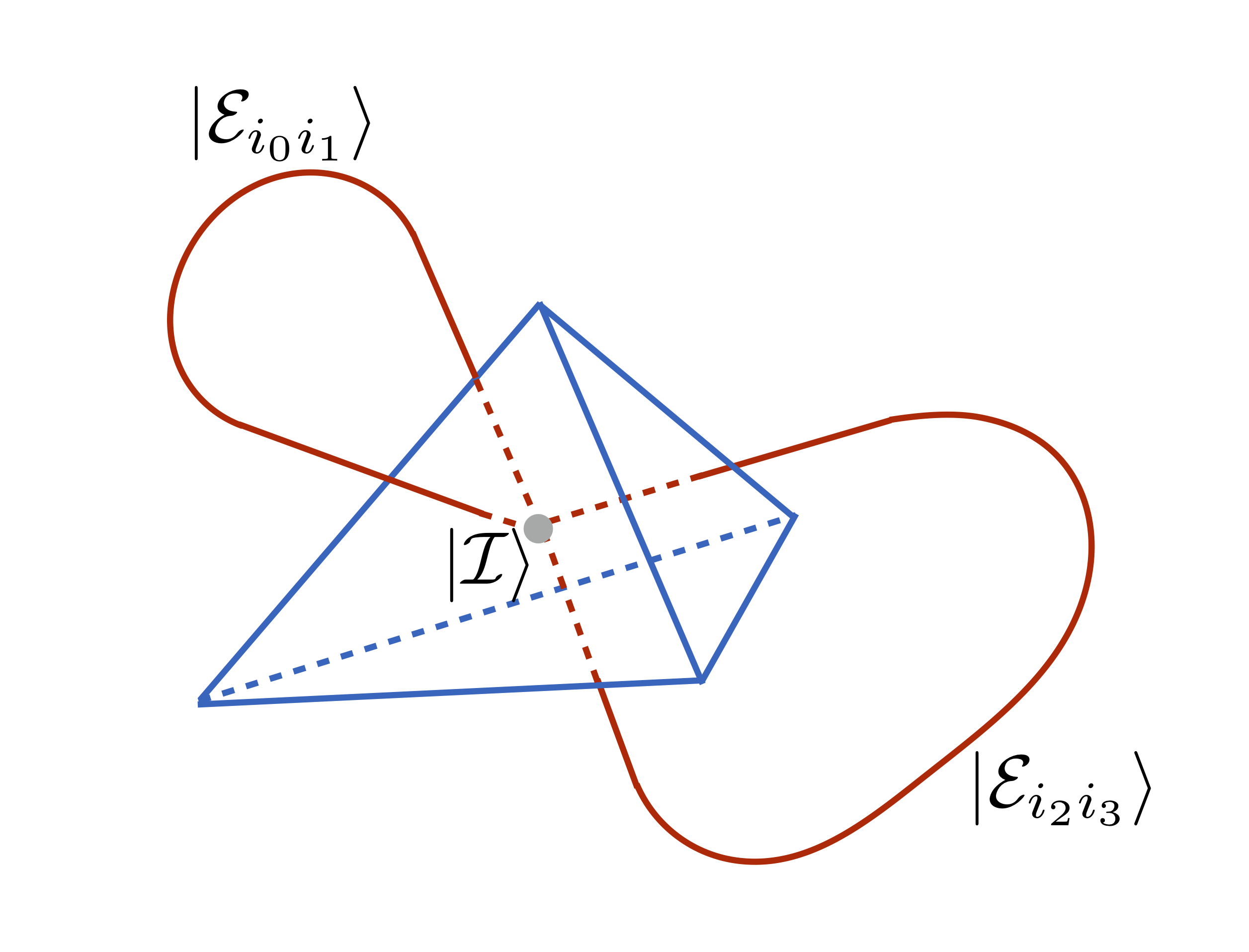
FIG. 18: Monopole spin network and the corresponding pairing of the faces of the dual tetrahedron.

In the considered case the states are satisfying the Gauss constraint, therefore:

$$\hat{P}_{\text{G}}|\mathcal{E}_{ijkl}\rangle=|\mathcal{E}_{ijkl}\rangle.$$ (80)

The $U$ and $V$ matrices used in the quantum circuits are:

$$U_{0123} =\left(\begin{array}[]{cc}0&1\\ -1&0\end{array}\right),V_{0123}=\frac{1}{\sqrt{2}}\left(\begin{array}[]{cc}-1&-1\\ 1&-1\end{array}\right),$$ (85)

$$U_{0213} =\frac{1}{\sqrt{2}}\left(\begin{array}[]{cc}1&1\\ -1&1\end{array}\right),V_{0213}=\left(\begin{array}[]{cc}0&-1\\ 1&0\end{array}\right),$$ (90)

$$U_{0312} =\frac{1}{\sqrt{2}}\left(\begin{array}[]{cc}1&1\\ -1&1\end{array}\right),V_{0312}=\left(\begin{array}[]{cc}-1&0\\ 0&-1\end{array}\right).$$ (95)

In Fig. 19 a quantum circuit associated with the amplitude $\langle\mathcal{I}|\mathcal{E}_{0312}\rangle$ is presented.

FIG. 19: A quantum circuit for the transition amplitude $\langle\mathcal{I}|\mathcal{E}_{0312}\rangle$. Before reduction.

The circuit can be further reduced to the form show in Fig. 20.

FIG. 20: A quantum circuit for the transition amplitude $\langle\mathcal{I}|\mathcal{E}_{0312}\rangle$. After reduction.

Results of determination of probabilities $|\langle\mathcal{E}_{0312}|0_{s}\rangle|^{2}$ and $|\langle\mathcal{E}_{0312}|1_{s}\rangle|^{2}$ on Melbourne and Yorktown quantum computers are collected in Table 2. In both cases the reduced circuit shown in Fig 20 was ued.

$$\begin{array}[]{|c|c|c|c|}\hline\cr\text{Amplitude}&\text{Theory}&\text{Melbourne}&\text{Yorktown}\\ \hline\cr|\langle 0_{s}|\mathcal{E}_{0312}\rangle|^{2}&0.25&0.23\pm 0.01&0.22\pm 0.01\\ |\langle 1_{s}|\mathcal{E}_{0312}\rangle|^{2}&0.75&0.72\pm 0.01&0.67\pm 0.01\\ \hline\cr\end{array}$$

Table 2: Results of simulations for the monopole spin network.

In the simulations, a sequence of 10 computational rounds each containing 1024 shots was performed for every of the investigated states. The modulus squares of the amplitudes were determined using the method introduced in Sec. VI. In the considered case, satisfactory agreement between the outcomes of measurement and the theoretical predictions are found, with slightly better results obtained with the use of the Melbourne quantum processor.

IX Dipole Spin Network

In the geometric picture, dipole spin network is obtained by considering two tetrahedra glued together face by face, as depicted in Fig. 21.

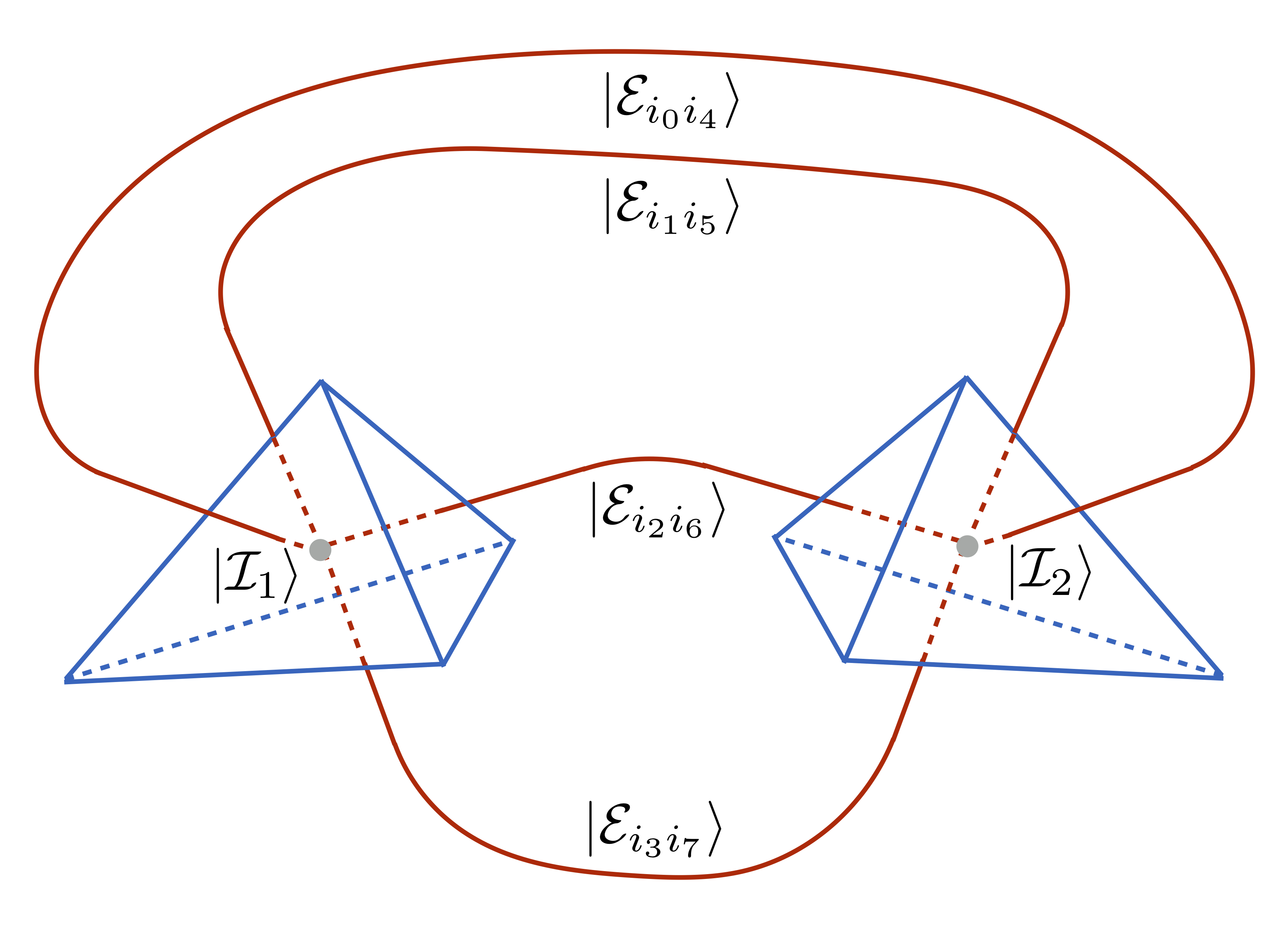
FIG. 21: Dipole spin network and the corresponding pairing of the faces of the dual tetrahedra.

Because, there are numerous possible permutations of the connections, there are various possible states of the maximally entangled states associated with the dipol diagram. The possible 24 configurations of connection and the corresponding states are summarized in Table 3.

$$\begin{array}[]{|c|c|c|c|c|}\hline\cr\text{Connections}&|0_{s}0_{s}\rangle&|0_{s}1_{s}\rangle&|1_{s}0_{s}\rangle&|1_{s}1_{s}\rangle\\ \hline\cr\{0,4\},\{1,5\},\{2,6\},\{3,7\}&\hbox{\multirowsetup$\frac{1}{4}$}&\hbox{\multirowsetup$0$}&\hbox{\multirowsetup$0$}&\hbox{\multirowsetup$\frac{1}{4}$}\\ \{0,5\},\{1,4\},\{2,7\},\{3,6\}&&&&\\ \{0,6\},\{1,7\},\{2,4\},\{3,5\}&&&&\\ \{0,7\},\{1,6\},\{2,5\},\{3,4\}&&&&\\ \hline\cr\{0,4\},\{1,5\},\{2,7\},\{3,6\}&\hbox{\multirowsetup$-\frac{1}{4}$}&\hbox{\multirowsetup$0$}&\hbox{\multirowsetup$0$}&\hbox{\multirowsetup$\frac{1}{4}$}\\ \{0,5\},\{1,4\},\{2,6\},\{3,7\}&&&&\\ \{0,6\},\{1,7\},\{2,5\},\{3,4\}&&&&\\ \{0,7\},\{1,6\},\{2,4\},\{3,5\}&&&&\\ \hline\cr\{0,4\},\{1,6\},\{2,5\},\{3,7\}&\hbox{\multirowsetup$\frac{1}{8}$}&\hbox{\multirowsetup$\frac{\sqrt{3}}{8}$}&\hbox{\multirowsetup$\frac{\sqrt{3}}{8}$}&\hbox{\multirowsetup$-\frac{1}{8}$}\\ \{0,5\},\{1,7\},\{2,4\},\{3,6\}&&&&\\ \{0,6\},\{1,4\},\{2,7\},\{3,5\}&&&&\\ \{0,7\},\{1,5\},\{2,6\},\{3,4\}&&&&\\ \hline\cr\{0,4\},\{1,6\},\{2,7\},\{3,5\}&\hbox{\multirowsetup$-\frac{1}{8}$}&\hbox{\multirowsetup$-\frac{\sqrt{3}}{8}$}&\hbox{\multirowsetup$\frac{\sqrt{3}}{8}$}&\hbox{\multirowsetup$-\frac{1}{8}$}\\ \{0,5\},\{1,7\},\{2,6\},\{3,4\}&&&&\\ \{0,6\},\{1,4\},\{2,5\},\{7,3\}&&&&\\ \{0,7\},\{1,5\},\{2,4\},\{6,3\}&&&&\\ \hline\cr\{0,4\},\{1,7\},\{2,5\},\{3,6\}&\hbox{\multirowsetup$-\frac{1}{8}$}&\hbox{\multirowsetup$\frac{\sqrt{3}}{8}$}&\hbox{\multirowsetup$-\frac{\sqrt{3}}{8}$}&\hbox{\multirowsetup$-\frac{1}{8}$}\\ \{0,5\},\{1,6\},\{2,4\},\{3,7\}&&&&\\ \{0,6\},\{1,5\},\{2,7\},\{3,4\}&&&&\\ \{0,7\},\{1,4\},\{2,6\},\{3,5\}&&&&\\ \hline\cr\{0,4\},\{1,7\},\{2,6\},\{3,5\}&\hbox{\multirowsetup$\frac{1}{8}$}&\hbox{\multirowsetup$-\frac{\sqrt{3}}{8}$}&\hbox{\multirowsetup$-\frac{\sqrt{3}}{8}$}&\hbox{\multirowsetup$-\frac{1}{8}$}\\ \{0,5\},\{1,6\},\{2,7\},\{3,4\}&&&&\\ \{0,6\},\{1,5\},\{2,4\},\{3,7\}&&&&\\ \{0,7\},\{1,4\},\{2,5\},\{3,6\}&&&&\\ \hline\cr\end{array}$$

Table 3: Amplitudes of the projected states for the 24 combinations of connections for the dipol diagram.

As an example, we will consider the following state:

$$|\mathcal{E}_{04152637}\rangle=|\mathcal{E}_{04}\rangle|\mathcal{E}_{15}\rangle|\mathcal{E}_{26}\rangle|\mathcal{E}_{37}\rangle,$$ (96)

which corresponds to the connections $\{\{0,4\},\{1,5\},\{2,6\},\{3,7\}\}$. Projecting the state onto the spin network basis (imposing the Gauss constraint) gives,

$$\hat{P}_{\text{G}}|\mathcal{E}_{04152637}\rangle=\frac{1}{4}\left(|0_{s}0_{s}\rangle+|1_{s}1_{s}\rangle\right)$$ (97)

such that in consequence, we have the two non-vanishing amplitudes:

$$\langle 0_{s}0_{s}|\mathcal{E}_{04152637}\rangle=\langle 1_{s}1_{s}|\mathcal{E}_{04152637}\rangle=\frac{1}{4},$$ (98)

$$\langle 0_{s}1_{s}|\mathcal{E}_{04152637}\rangle=\langle 1_{s}0_{s}|\mathcal{E}_{04152637}\rangle=0.$$ (99)

From the viewpoint of quantum computing, the amplitudes can be determined by evaluating the quantum circuit presented in Fig. 22.

FIG. 22: A quantum circuit for transition amplitude $\langle\mathcal{I}_{1}\mathcal{I}_{2}|\mathcal{E}_{04152637}\rangle$.

For the special case of the states of the interwiners $|\mathcal{I}_{1}\mathcal{I}_{2}\rangle=|0_{s}0_{s}\rangle$ the quantum circuit can be simplified to the form presented in Fig. 23, where representation of the state $|0_{s}\rangle$ by the circuit (11) has been used.

FIG. 23: Simplified version of a quantum circuit for transition amplitude $\langle 0_{s}0_{s}|\mathcal{E}_{04152637}\rangle$.

The circuits can be directly embedded into the architecture of the Melbourne quantum processors, shown in Fig. 7. Results of our simulations are collected in Table 4.

$$\begin{array}[]{|c|c|c|c|}\hline\cr\text{Amplitude}&\text{Theory}&\text{Melbourne}&\text{Melbourne - S}\\ \hline\cr|\langle 0_{s}0_{s}|\mathcal{E}_{04152637}\rangle|^{2}&0.0625&0.008\pm 0.002&0.003\pm 0.001\\ |\langle 0_{s}1_{s}|\mathcal{E}_{04152637}\rangle|^{2}&0&0.003\pm 0.002&-\\ |\langle 1_{s}0_{s}|\mathcal{E}_{04152637}\rangle|^{2}&0&0.009\pm 0.002&-\\ |\langle 1_{s}1_{s}|\mathcal{E}_{04152637}\rangle|^{2}&0.0625&0.008\pm 0.003&-\\ \hline\cr\end{array}$$

Table 4: Results of simulations for the dipole network on the 15 qubit Melbourne quantum computer.

As previously, a sequence of 10 computational rounds each containing 1024 shots was performed for every of the investigated states. Eight out of fifteen qubits of the Melbourne processor have been used in the computations. The third column of Table 4 contains results of simulations based on the circuit shown in Fig. 22) whereas the fourth column presents result obtained using the circuit shown in Fig. 23. The obtained results differ cardinally from the theoretical predictions. The reason for this is most probably significant depth of the considered quantum circuits and accumulations of errors. In order to better understand this issue in the employed quantum chip a set of test have been performed. Results of the tests are collected in Appendix B. One can find that significant accumulation of errors is present even for simple low-depth circuits. This indicates, that going beyond the case of a single node (with the use of currently available quantum processors) cannot be done successfully without adopting quantum error correction codes.

X Summary

Loop quantum gravity and related approaches to gravity, such as Group Field Theories, provide picture of spacetime as a many-body quantum system Oriti:2017twl . The degrees of freedom are associated with the quanta of volume (“atoms of space”) related to the nodes of a spin network. This viewpoint opens an interesting possibility to employ many-body quantum physics methods designed to explore complex collective properties of composite systems. Especially promising paths to include: tensor networks methods and quantum simulations.

In this article, the second method has been discussed, following the ideas developed in Refs. Li:2017gvt ; Mielczarek:2018ttq ; Mielczarek:2018jsh . Primarily, our focus was on construction of a quantum circuit for a general intertwiner qubit state. Such circuit has been introduced and shown to utilize four logical qubits, without involving quantum error correction codes. The presented circuit is a generalization of the circuit for the basis state $|0_{s}\rangle$ explored in Ref. Mielczarek:2018jsh . Based on the circuit, exemplary intertwiner qubits states were simulated on both 5-qubit (Yorktown) and 15-qubit (Melbourne) IBM superconducting quantum processors. It has been shown that for the case of the 5-qubit machine, fidelities of the obtained states reach the level of $F\approx 90$ %. On the other hand, while the total number of qubits of the processor is increased to 15, the fidelity of the states drops down to $F\approx 85$ %, even if the number of utilized logical qubits remains to be four. This is a first sign of the fact that it is much more difficult to keep quantum coherence of bigger quantum systems. Further, even more drastic, consequences of this fact have beed observed while transition amplitudes between simple spin network states were studied.

For this purpose, a class of maximally entangled spin network states, analogous to the PEPS tensor networks, has been introduced. The states have been introduced by considering maximally entangled states between source and target Hilbert spaces of holonomies, corresponding to links of the spin network. Such possibility is supported by recent results presented in Ref. Mielczarek:2019srn . Furthermore, the state of maximally entangled links has to be projected onto the surface of Gauss constraint in order to get well defined superposition of spin network states. With the use of such appropriately projected state, exemplary transition amplitudes for a monopole and dipole spin networks have been considered.

The monopole spin network amplitudes required only four logical qubits, and runs of the associated quantum circuit on a superconducting 5-qubit chip lead to good agreement with theoretical predictions. On the other hand, the dipole spin network involves 8 logical qubits, and the associated quantum circuit was transpilated to the form compatible with topology of the available 15 qubit IBM quantum processor. However, because of significant errors, running of the circuit on the quantum computer did not lead to reasonable results. Therefore, for the moment, quantum simulations of the dipole spin networks are still challenging. This concerns the considered publicly available IBM superconducting quantum process, which has been used. However, the current hight activity in the quantum computing technologies prognosis that both the dipole and more complex spin networks will be possible simulate successfully in the coming years.

XI Acknowledgements

Authors are supported from the Sonata Bis Grant DEC-2017/26/E/ST2/00763 of the National Science Centre Poland. Furthermore, this publication was made possible through the support of the ID# 61466 grant from the John Templeton Foundation, as part of the “The Quantum Information Structure of Spacetime (QISS)” Project (qiss.fr). The opinions expressed in this publication are those of the authors and do not necessarily reflect the views of the John Templeton Foundation. Authors would also like to thank to Daniel Nagaj for discussion on the quantum circuits at the initial stage of the preparation of the article.

Appendix A

The appendix summarizes numerical data obtained from evaluation of the quantum circuits for the intertwiner qubit states on IBM superconducting quantum computers. For each of the considered case, 10 computational rounds have been performed each of 1024 shots (evaluation of quantum circuit and performing measurement). Both averages and standard deviations have been determined based on the 10 computational rounds.

In Table 5 the results of quantum simulations on the 5-qubit (Yorktown) IBM quantum computer are collected.

$$\begin{array}[]{|c|c|c|c|c|c|c|}\hline\cr\text{State}&|0_{s}\rangle&|1_{s}\rangle&|+\rangle&|-\rangle&|\circlearrowright\rangle&|\circlearrowleft\rangle\\ \hline\cr|0000\rangle&0.007\pm 0.001&0.021\pm 0.003&0.016\pm 0.005&0.008\pm 0.003&0.01\pm 0.003&0.009\pm 0.003\\ |0001\rangle&0.020\pm 0.002&0.014\pm 0.006&0.015\pm 0.004&0.016\pm 0.004&0.015\pm 0.004&0.02\pm 0.005\\ |0010\rangle&0.024\pm 0.006&0.024\pm 0.005&0.025\pm 0.006&0.028\pm 0.007&0.027\pm 0.005&0.022\pm 0.004\\ |0011\rangle&0.008\pm 0.003&0.305\pm 0.015&0.172\pm 0.008&0.128\pm 0.015&0.151\pm 0.014&0.142\pm 0.010\\ |0100\rangle&0.023\pm 0.007&0.016\pm 0.004&0.012\pm 0.003&0.025\pm 0.004&0.017\pm 0.005&0.022\pm 0.006\\ |0101\rangle&0.183\pm 0.011&0.066\pm 0.007&0.03\pm 0.004&0.243\pm 0.013&0.123\pm 0.012&0.150\pm 0.006\\ |0110\rangle&0.175\pm 0.012&0.048\pm 0.007&0.193\pm 0.010&0.026\pm 0.003&0.126\pm 0.01&0.099\pm 0.012\\ |0111\rangle&0.017\pm 0.004&0.009\pm 0.003&0.021\pm 0.005&0.007\pm 0.003&0.013\pm 0.005&0.011\pm 0.005\\ |1000\rangle&0.025\pm 0.005&0.021\pm 0.004&0.030\pm 0.006&0.018\pm 0.005&0.025\pm 0.005&0.026\pm 0.008\\ |1001\rangle&0.206\pm 0.013&0.069\pm 0.010&0.200\pm 0.016&0.059\pm 0.005&0.119\pm 0.007&0.158\pm 0.008\\ |1010\rangle&0.262\pm 0.012&0.077\pm 0.007&0.087\pm 0.005&0.277\pm 0.016&0.190\pm 0.009&0.160\pm 0.009\\ |1011\rangle&0.022\pm 0.006&0.014\pm 0.002&0.012\pm 0.004&0.024\pm 0.004&0.017\pm 0.004&0.021\pm 0.004\\ |1100\rangle&0.007\pm 0.003&0.278\pm 0.011&0.151\pm 0.01&0.119\pm 0.007&0.141\pm 0.011&0.138\pm 0.009\\ |1101\rangle&0.007\pm 0.003&0.010\pm 0.004&0.011\pm 0.003&0.010\pm 0.003&0.009\pm 0.004&0.007\pm 0.003\\ |1110\rangle&0.008\pm 0.002&0.008\pm 0.003&0.010\pm 0.003&0.005\pm 0.001&0.007\pm 0.003&0.006\pm 0.002\\ |1111\rangle&0.006\pm 0.002&0.020\pm 0.003&0.015\pm 0.003&0.007\pm 0.002&0.011\pm 0.005&0.011\pm 0.002\\ \hline\cr\end{array}$$

Table 5: Experimental results for the states generated on 5-qubit (Yorktown) IBM quantum computer.

In Table 6 the results of quantum simulations on the 15-qubit (Melbourne) IBM quantum computer are collected.

$$\begin{array}[]{|c|c|c|c|c|c|c|}\hline\cr\text{State}&|0_{s}\rangle&|1_{s}\rangle&|+\rangle&|-\rangle&|\circlearrowright\rangle&|\circlearrowleft\rangle\\ \hline\cr|0000\rangle&0.04\pm 0.005&0.019\pm 0.003&0.043\pm 0.005&0.013\pm 0.003&0.026\pm 0.005&0.024\pm 0.006\\ |0001\rangle&0.033\pm 0.005&0.053\pm 0.008&0.05\pm 0.007&0.035\pm 0.008&0.041\pm 0.006&0.05\pm 0.006\\ |0010\rangle&0.033\pm 0.006&0.033\pm 0.006&0.026\pm 0.005&0.042\pm 0.006&0.036\pm 0.007&0.034\pm 0.004\\ |0011\rangle&0.025\pm 0.005&0.239\pm 0.012&0.109\pm 0.008&0.119\pm 0.011&0.096\pm 0.009&0.16\pm 0.008\\ |0100\rangle&0.034\pm 0.005&0.043\pm 0.007&0.032\pm 0.005&0.039\pm 0.006&0.034\pm 0.006&0.035\pm 0.007\\ |0101\rangle&0.128\pm 0.011&0.105\pm 0.009&0.033\pm 0.005&0.225\pm 0.014&0.158\pm 0.014&0.085\pm 0.011\\ |0110\rangle&0.246\pm 0.015&0.063\pm 0.006&0.244\pm 0.011&0.055\pm 0.007&0.156\pm 0.011&0.158\pm 0.008\\ |0111\rangle&0.028\pm 0.005&0.014\pm 0.002&0.018\pm 0.006&0.026\pm 0.003&0.017\pm 0.004&0.02\pm 0.004\\ |1000\rangle&0.029\pm 0.006&0.02\pm 0.005&0.025\pm 0.005&0.026\pm 0.003&0.026\pm 0.004&0.026\pm 0.006\\ |1001\rangle&0.166\pm 0.019&0.065\pm 0.008&0.207\pm 0.015&0.037\pm 0.007&0.129\pm 0.009&0.126\pm 0.007\\ |1010\rangle&0.135\pm 0.013&0.065\pm 0.009&0.035\pm 0.007&0.217\pm 0.015&0.148\pm 0.008&0.082\pm 0.007\\ |1011\rangle&0.011\pm 0.004&0.024\pm 0.006&0.014\pm 0.004&0.022\pm 0.005&0.016\pm 0.004&0.017\pm 0.003\\ |1100\rangle&0.024\pm 0.005&0.204\pm 0.016&0.094\pm 0.008&0.1\pm 0.007&0.064\pm 0.011&0.126\pm 0.009\\ |1101\rangle&0.014\pm 0.004&0.018\pm 0.004&0.012\pm 0.006&0.021\pm 0.005&0.016\pm 0.005&0.015\pm 0.003\\ |1110\rangle&0.023\pm 0.007&0.018\pm 0.003&0.027\pm 0.008&0.012\pm 0.003&0.019\pm 0.005&0.022\pm 0.002\\ |1111\rangle&0.031\pm 0.006&0.016\pm 0.005&0.03\pm 0.004&0.012\pm 0.004&0.017\pm 0.003&0.02\pm 0.005\\ \hline\cr\end{array}$$

Table 6: Experimental results for the states generated on 15-qubit (Melbourne) IBM quantum computer.

For comparison, in Table 7 theoretical values of the probabilities of the basis states for the states under consideration are shown.

$$\begin{array}[]{|c|c|c|c|c|c|c|}\hline\cr\text{State}&|0_{s}\rangle&|1_{s}\rangle&|+\rangle&|-\rangle&|\circlearrowright\rangle&|\circlearrowleft\rangle\\ \hline\cr|0000\rangle&0.0&0.0&0.0&0.0&0.0&0.0\\ |0001\rangle&0.0&0.0&0.0&0.0&0.0&0.0\\ |0010\rangle&0.0&0.0&0.0&0.0&0.0&0.0\\ |0011\rangle&0.0&0.333&0.167&0.167&0.167&0.167\\ |0100\rangle&0.0&0.0&0.0&0.0&0.0&0.0\\ |0101\rangle&0.25&0.083&0.022&0.311&0.167&0.167\\ |0110\rangle&0.25&0.083&0.311&0.022&0.167&0.167\\ |0111\rangle&0.0&0.0&0.0&0.0&0.0&0.0\\ |1000\rangle&0.0&0.0&0.0&0.0&0.0&0.0\\ |1001\rangle&0.25&0.083&0.311&0.022&0.167&0.167\\ |1010\rangle&0.25&0.083&0.022&0.311&0.167&0.167\\ |1011\rangle&0.0&0.0&0.0&0.0&0.0&0.0\\ |1100\rangle&0.0&0.333&0.167&0.167&0.167&0.167\\ |1101\rangle&0.0&0.0&0.0&0.0&0.0&0.0\\ |1110\rangle&0.0&0.0&0.0&0.0&0.0&0.0\\ |1111\rangle&0.0&0.0&0.0&0.0&0.0&0.0\\ \hline\cr\end{array}$$

Table 7: Theoretical probabilities for the states under consideration.

Appendix B

The appendix summarizes tests performed on the 15 qubits IBM quantum processor Melbourne. The following four tests have been performed:

1. Measurements on $n$ qubits without any quantum gates applied (the $\otimes_{i=1}^{15}|0\rangle$ state).

2. Applying NOT gates ($\hat{X}$) and measurement on $n$ qubits.

3. Applying NOT gates on all 15 qubits and performing measurement on $n$ first qubits.

4. Applying NOT gates on $n$ qubits and performing measurement on all 15 qubits.

In Fig. 24 fidelities for the states obtained for the four test are presented. The presented data are collected in Table 8.

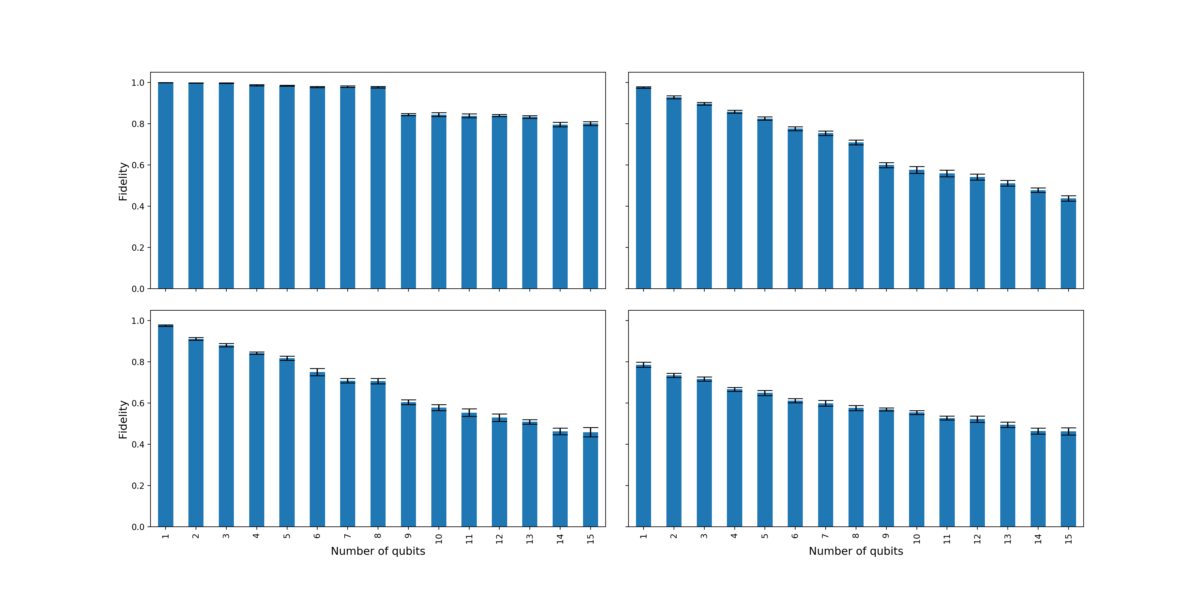
FIG. 24: Fidelities for the four types of tests performed on the 15-qubit Melbourne quantum computer. From top left: measures on $n$ qubits for the empty quantum register, NOT gates and measures on $n$ qubits, NOT gates on all 15 qubits and measurement on $n$ qubits, NOT gates on $n$ qubits and measuremen on all 15 qubits.

$$\begin{array}[]{|c|c|c|c|c|}\hline\cr n&1^{st}\ \text{test}&2^{nd}\ \text{test}&3^{rd}\ \text{test}&4^{th}\ \text{test}\\ \hline\cr 1&1.000\pm 0.000&0.976\pm 0.003&0.976\pm 0.003&0.786\pm 0.012\\ 2&0.998\pm 0.001&0.928\pm 0.007&0.911\pm 0.006&0.734\pm 0.010\\ 3&0.997\pm 0.002&0.897\pm 0.007&0.881\pm 0.008&0.717\pm 0.011\\ 4&0.987\pm 0.003&0.859\pm 0.007&0.843\pm 0.006&0.667\pm 0.009\\ 5&0.985\pm 0.002&0.825\pm 0.008&0.818\pm 0.010&0.649\pm 0.012\\ 6&0.979\pm 0.003&0.776\pm 0.009&0.751\pm 0.018&0.611\pm 0.010\\ 7&0.980\pm 0.004&0.755\pm 0.011&0.709\pm 0.011&0.599\pm 0.014\\ 8&0.978\pm 0.004&0.710\pm 0.012&0.707\pm 0.013&0.576\pm 0.013\\ 9&0.844\pm 0.006&0.600\pm 0.013&0.604\pm 0.012&0.569\pm 0.008\\ 10&0.845\pm 0.009&0.576\pm 0.017&0.579\pm 0.015&0.554\pm 0.009\\ 11&0.839\pm 0.010&0.560\pm 0.016&0.554\pm 0.018&0.528\pm 0.009\\ 12&0.840\pm 0.005&0.542\pm 0.015&0.529\pm 0.018&0.522\pm 0.015\\ 13&0.834\pm 0.007&0.512\pm 0.014&0.509\pm 0.011&0.495\pm 0.013\\ 14&0.797\pm 0.011&0.478\pm 0.011&0.463\pm 0.017&0.464\pm 0.015\\ 15&0.801\pm 0.010&0.438\pm 0.014&0.459\pm 0.023&0.463\pm 0.017\\ \hline\cr\end{array}$$

Table 8: Fidelities of states for the four tests performed on the 15 qubit IBM quantum computer (Melbourne).

References

- (1) K. Li et al., Communications Physics, volume 2, Article number: 122 (2019) [arXiv:1712.08711 [quant-ph]].
- (2) J. Mielczarek, arXiv:1801.06017 [gr-qc].
- (3) J. Mielczarek, arXiv:1803.10592 [gr-qc].
- (4) J. Mielczarek, Universe 5 (2019) no.8, 179 [arXiv:1810.07100 [gr-qc]].
- (5) L. Cohen, A. J. Brady, Z. Huang, H. Liu, D. Qu, J. P. Dowling and M. Han, arXiv:2003.03414 [quant-ph].
- (6) P. Zhang, Z. Huang, C. Song, Q. Guo, Z. Song, H. Dong, Z. Wang, L. Hekang, M. Han and H. Wang, et al. [arXiv:2007.13682 [quant-ph]].
- (7) A. Ashtekar and J. Lewandowski, Class. Quant. Grav. 21 (2004) R53 [gr-qc/0404018].
- (8) C. Rovelli, Living Rev. Rel. 1 (1998) 1 [gr-qc/9710008].
- (9) F. Arute, K. Arya, R. Babbush, et al., Nature 574, 505-510 (2019).
- (10) S. Ryu and T. Takayanagi, Phys. Rev. Lett. 96 (2006) 181602 [hep-th/0603001].
- (11) B. Swingle, Phys. Rev. D 86 (2012) 065007 [arXiv:0905.1317 [cond-mat.str-el]].
- (12) L. Susskind, arXiv:1708.03040 [hep-th].
- (13) L. Susskind, J. Math. Phys. 36 (1995), 6377-6396 [arXiv:hep-th/9409089 [hep-th]].
- (14) J. M. Maldacena, Int. J. Theor. Phys. 38 (1999) 1113 [Adv. Theor. Math. Phys. 2 (1998) 231].
- (15) M. Han and L. Y. Hung, Phys. Rev. D 95 (2017) no.2, 024011.
- (16) K. Li, M. Han, D. Qu, Z. Huang, G. Long, Y. Wan, D. Lu, B. Zeng and R. Laflamme, npj Quantum Inf. 5 (2019), 30 [arXiv:1705.00365 [quant-ph]].
- (17) A. Feller and E. R. Livine, Phys. Rev. D 95 (2017) no.12, 124038 [arXiv:1703.01156 [hep-th]].
- (18) C. Rovelli, F. Vidotto, “Covariant Loop Quantum Gravity: An Elementary Introduction to Quantum Gravity and Spinfoam Theory,” Cambridge Monographs on Mathematical Physics, 2014.
- (19) G. Immirzi, Nucl. Phys. B Proc. Suppl. 57 (1997), 65-72 [arXiv:gr-qc/9701052 [gr-qc]].
- (20) J. F. Barbero G., Phys. Rev. D 51 (1995), 5507-5510 [arXiv:gr-qc/9410014 [gr-qc]].
- (21) A. Perez and C. Rovelli, Phys. Rev. D 73 (2006), 044013 [arXiv:gr-qc/0505081 [gr-qc]].
- (22) L. Freidel, D. Minic and T. Takeuchi, Phys. Rev. D 72 (2005), 104002 [arXiv:hep-th/0507253 [hep-th]].
- (23) A. Ashtekar, J. Baez, A. Corichi and K. Krasnov, Phys. Rev. Lett. 80 (1998), 904-907 [arXiv:gr-qc/9710007 [gr-qc]].
- (24) K. A. Meissner, Class. Quant. Grav. 21 (2004), 5245-5252 [arXiv:gr-qc/0407052 [gr-qc]].
- (25) I. Agullo, J. Fernando Barbero, E. F. Borja, J. Diaz-Polo and E. J. S. Villasenor, Phys. Rev. D 82 (2010), 084029 [arXiv:1101.3660 [gr-qc]].
- (26) A. Feller and E. R. Livine, Class. Quant. Grav. 33 (2016) no.6, 065005.
- (27) C. Rovelli and L. Smolin, Nucl. Phys. B 442 (1995) 593 Erratum: [Nucl. Phys. B 456 (1995) 753] [gr-qc/9411005].
- (28) A. Ashtekar and J. Lewandowski, Adv. Theor. Math. Phys. 1 (1998) 388 [gr-qc/9711031].
- (29) S. Bartlett, T. Rudolph and R. Spekkens, Phys. Rev. Lett. 91, 027901 (2003).
- (30) E. R. Livine and D. R. Terno, Nucl. Phys. B 741 (2006), 131-161 [arXiv:gr-qc/0508085 [gr-qc]].
- (31) https://quantum-computing.ibm.com/
- (32) A. Barenco et al., Phys.Rev. A 52 (1995) 3457.
- (33) J.Chen, F. Zhang, C.Huang, M. Newman and Y. Shi, arXiv:1805.01450 [quant-ph].
- (34) https://ai.google/research/teams/applied-science/quantum-ai/
- (35) https://www.rigetti.com/
- (36) https://ionq.co/
- (37) E. Magesan, J.M. Gambetta, J. Emerson Physical Review A 85.4 (2012): 042311. arXiv:1109.6887 [quant-ph]
- (38) D. Lidar and T. Brun, ed. (2013). “Quantum Error Correction”. Cambridge University Press.
- (39) https://qiskit.org/textbook/ch-quantum-hardware/measurement-error-mitigation.html
- (40) W. Donnelly, Phys. Rev. D 77 (2008), 104006 [arXiv:0802.0880 [gr-qc]].
- (41) W. Donnelly and L. Freidel, JHEP 09 (2016), 102 [arXiv:1601.04744 [hep-th]].
- (42) A. Feller and E. R. Livine, Class. Quant. Grav. 35 (2018) no.4, 045009 [arXiv:1710.04473 [gr-qc]].
- (43) E. R. Livine, Phys. Rev. D 97 (2018) no.2, 026009 [arXiv:1709.08511 [gr-qc]].
- (44) B. Czech, J. De Boer, D. Ge and L. Lamprou, JHEP 1911 (2019) 094 [arXiv:1903.04493 [hep-th]].
- (45) J. Mielczarek and T. Trześniewski, Phys. Lett. B 810 (2020), 135808 [arXiv:1911.10208 [hep-th]].
- (46) J.I. Cirac, and F. Verstraete, J. Phys. A: Math. Theor. 42, 504004 (2009)
- (47) F. Verstraete, V. Murg and J.I. Cirac, Advances in Physics, 57:2, 143-224 (2008)
- (48) R. Orus, Annals Phys. 349 (2014) 117 [arXiv:1306.2164 [cond-mat.str-el]].
- (49) J. Biamonte, arxiv:1912.10049 [quant-ph]
- (50) B. Baytas, E. Bianchi and N. Yokomizo, Phys. Rev. D 98 (2018) no.2, 026001 [arXiv:1805.05856 [gr-qc]].
- (51) E. Bianchi, P. Doná and I. Vilensky, Phys. Rev. D 99 (2019) no.8, 086013 [arXiv:1812.10996 [gr-qc]].
- (52) C. Rovelli and F. Vidotto, Class. Quant. Grav. 25 (2008), 225024 [arXiv:0805.4585 [gr-qc]].
- (53) E. F. Borja, J. Diaz-Polo, I. Garay and E. R. Livine, Class. Quant. Grav. 27 (2010), 235010 [arXiv:1006.2451 [gr-qc]].
- (54) E. Bianchi, C. Rovelli and F. Vidotto, Phys. Rev. D 82 (2010), 084035 [arXiv:1003.3483 [gr-qc]].
- (55) D. Oriti, L. Sindoni and E. Wilson-Ewing, Class. Quant. Grav. 33 (2016) no.22, 224001 [arXiv:1602.05881 [gr-qc]].
- (56) D. Oriti, arXiv:1710.02807 [gr-qc].