Statistical Quantile Learning for
Large, Nonlinear, and Additive Latent Variable Models

Abstract

The studies of large-scale, high-dimensional data in fields such as genomics and neuroscience have injected new insights into science. Yet, despite advances, they are confronting several challenges, often simultaneously: lack of interpretability, nonlinearity, slow computation, inconsistency and uncertain convergence, and small sample sizes compared to high feature dimensions. Here, we propose a relatively simple, scalable, and consistent nonlinear dimension reduction method that can potentially address these issues in unsupervised settings. We call this method Statistical Quantile Learning (SQL) because, methodologically, it leverages on a quantile approximation of the latent variables together with standard nonparametric techniques (sieve or penalyzed methods). We show that estimating the model simplifies into a convex assignment matching problem; we derive its asymptotic properties; we show that the model is identifiable under few conditions. Compared to its linear competitors, SQL explains more variance, yields better separation and explanation, and delivers more accurate outcome prediction. Compared to its nonlinear competitors, SQL shows considerable advantage in interpretability, ease of use and computations in large-dimensional settings. Finally, we apply SQL to high-dimensional gene expression data (consisting of $20,263$ genes from $801$ subjects), where the proposed method identified latent factors predictive of five cancer types. The SQL package is available at https://github.com/jbodelet/SQL.

Keywords: High-dimensionality, Nonlinear model, Latent variable model, Generative models, Dimension reduction, GAN, VAE, Nonparametric estimation, Assignment Matching, Prediction.

1 Introduction

Recent progress in science has witnessed increasingly large and complex datasets. While larger and more complex datasets generally encode more information, they bring about unique statistical and scientific challenges. First, these data are high-dimensional, oftentimes with dimensionality much larger than the sample size. If not accounted for, traditional statistical methods may result in non-unique solutions. Second, these data are often nonlinear, not only between features, but also between features and outcomes. While linear models may still identify some effects, their estimates may be prone to bias or result in misidentification, and sometimes both.

A common way to deal with the first issue is to use dimensionality reduction. By condensing and summarizing information into a small number of features, it effectively reduces data size, facilitates explanation and visualization, and, when estimation is concerned, may yield unique solutions. Such attractive properties, therefore, have interested machine learning scientists, biologists and engineers, not to mention statisticians. Traditional dimension reduction tools, such as Principal Component Analysis (PCA) and Factor Analysis (FA), however, assume linearity and therefore are adequate for features that are (at least approximately) linear. For nonlinear data, these methods may fail, even with minor perturbations. For example, consider million of single nucleotide polymorphisms (SNPs) in genomics research and hundreds of thousands of voxels (brain areas) in neuroimaging studies. The SNP-to-SNP and voxel-to-voxel relationships are high-dimensional and nonlinear (Becht et al.,, 2019). Additionally, when (disease) outcome prediction is concerned, the relationship between the genes and the outcome and that between brain regions and the outcome are also high-dimensional and nonlinear. The problem is further compounded when such data are usually only available in a few dozens or hundreds of subjects, a number that is much smaller than that of the features. Although progresses are already being made (Lee et al.,, 2007, Van der Maaten and Hinton,, 2008, McInnes et al.,, 2018) there is a pressing need for interpretable nonlinear dimension reduction and prediction techniques for large-scale and high-dimensional data.

Nonlinear latent variable models, as they generalize factor analysis, have sparked the interest of both the statistical and the machine learning communities, in the form of nonlinear factor models in statistical science and (deep) generative models in machine learning. Nonlinear factor models (see Amemiya and Yalcin,, 2002 and reference therein) usually rely on a parametric form. The deep generative models, on the other hand, rely on deep neural networks (DNN). These latter are known to be universal functional approximators (Hornik et al.,, 1989) and belong to the class of sieve estimators although their asymptotic behavior are not fully understood (see Shen et al., (2019)). To estimate the deep generative models, there are two main general approaches: a variational approach, also known as variational autoencoders (VAE), see Kingma and Welling, (2014), and a simulation-based approach, called the Generative Adversarial Networks (GAN), see Goodfellow et al., (2014). These methods rely on a double DNN specification. A first DNN model the conditional distribution of the features given latent variables (often called the “generator”), while a second DNN is used to recover the latent space. In VAE, an encoder function directly maps the data to the latent space by approximating the posterior distribution of the latent variables (see Kingma and Welling,, 2014 and Doersch,, 2016 for a detailed review). In GAN, one performs inference implicitly using a discriminator.

While both nonlinear factor models and deep generative models have advanced the analysis of high-dimensional nonlinear data, they are facing crucial methodological, and computational challenges. For nonlinear factors models, they lack nonparametric inferences. For deep generative models, while they are effective, especially given large sample sizes, and can potentially better handle the curse of dimensionality, to accurately recover the discriminator (e.g., in GAN) or the encoder (e.g., in VAE), both nonparametric functions of the $p$-dimensional data, is prohibitively difficult for large dimensional and high-dimensional ($p>n$) scenarios (Poggio et al.,, 2017, Bauer and Kohler,, 2019). Additionally, deep learning methods suffer from several drawbacks, preventing a wide acceptance in the statistical community. For example, the estimators are very sensitive to the choice of the hyperparameters and training suffer from issues such as the vanishing gradient problem and mode collapse. From a practical point, the use of the double neural networks can sometimes make their training difficult, especially for GANs. Even more importantly, the parameters of the generator, often of main interest in science, are not uniquely identified for deep generative models and therefore are hard to interpret: due to these challenges, the deep generative models are often referred to as “black boxes”.

Here, to address these challenges, we introduce the Statistical Quantile Learning (SQL), a new nonparametric estimation method, that

1. Deals with the general, dual problems of nonlinearity and the curse of dimensionality in large and high-dimensional nonlinear data analysis;

2. Warrants identifiable and consistent estimates, with an asymptotic guarantee and fast convergence rate in large and high-dimensional settings.

3. Overcomes the restriction of parametric assumptions in nonlinear factor models in statistics and the difficulty of hyperparameter specification and training in deep learning.

4. Achieves better separation and explains more variability than linear competitors, such as PCA, in unsupervised learning.

5. Outperforms VAE in large and high-dimensional settings and is competitive to VAE in low-dimensional settings.

Before presenting the general method in Section 2 and its theory in Section 3, here we first outline the model in relatively simple terms and summarise the attractive theoretical findings in words. We consider $p$-dimensional data $\bm{X}$ and the model $\bm{X}=\bm{f}({\bm{Z}})+\bm{\epsilon}$, where $\bm{\epsilon}$ is a random errors vector and ${\bm{Z}}\in\mathcal{Z}^{q}$ is a $q$-dimensional unobserved latent variable. The dimension $q$ is usually assumed to be much smaller than $p$ for dimension reduction purpose. The unknown function $\bm{f}:\mathcal{Z}^{q}\rightarrow\mathbb{R}^{p}$ is called the generator. We restrict the generator to additive functions. This avoids the curse of dimensionality when the number of latent variables $q$ is large and offers more interpretability. The factors can come from some fixed distribution, usually the normal or uniform distribution.

The key idea of the SQL method is to approximate the latent factors by their quantiles. We show that finding these “latent quantiles” renders to solving an assignment matching problem. The generator is estimated using standard statistical nonparametric techniques, such as sieve and penalyzed methods. This framework allows us to investigate the rates of convergence of the SQL estimates using empirical process theory (van de Geer, 2000b, , Van der Vaart,, 2000) for both sieve and penalyzed estimators under weak conditions. Critically, we find that the rates of convergence improve as both the sample size and the dimension of the features increase. In particular, when the dimension $p$ is large, the SQL estimates reach the classical rates of convergence as if the latent factors were known and thus enjoy the “blessing of dimensionality”.

The rest of the article is organized as follows. In Section 2, we introduce the model and the estimation method for SQL. In Section 3, we discuss the theoretical properties of the model and of the estimators. In Section 4, we illustrate the finite sample performance of the estimators using simulation studies. In Section 5, we apply SQL to high-dimensional gene expression data from cancer patients and use the extracted latent features to predict five cancer types.

2 Method

2.1 The model

We consider $p$-dimensional observations $\bm{X}_{1},\dots,\bm{X}_{n}\in\mathbb{R}^{p}$. Suppose that the observations are associated to unobserved $q$-dimensional latent factors $\bm{Z}_{i}=(Z_{i,1},\dots,Z_{i,q})\in\mathcal{Z}^{q}$ through an additive generator, i.e., $f_{j}(\cdot):=\mu_{j}+\sum_{l=1}^{q}f_{j,l}(\cdot)$, satisfying the following model:

$$X_{i,j}=\mu_{j}+\sum_{l=1}^{q}f_{j,l}(Z_{i,l})+\epsilon_{i,j},\quad i=1,\dots,n,\quad j=1,\dots,p$$ (1)

where $\bm{\epsilon}_{i,j}$ are mutually independent random errors and independant of ${\bm{Z}}_{i}$. Moreover, following the convention in the literature, we assume the identifiability condition that

$$\mathbb{E}(f_{{j,l}}(Z_{i,l}))=0,\text{for all }j=1,...,p\text{ and }l=1,\dots,q.$$

The assumption implies that $\mathbb{E}[X_{ij}]=\mu_{j}$. Without loss of generality, we assume that the observations $X_{i,j}$ are centered and that $\mu_{j}=0$. To build our estimation, we assume the following two reasonable, but key assumptions on the latent factors and the generators.

Assumption A1.

(Assumption on the latent factors). For each $l\in\{1,\dots,q\}$, the latent factors $\{Z_{i,l}\}_{i=1}^{n}$ have marginal cumulative distribution function (CDF) $P_{Z}^{(l)}:\mathcal{Z}\rightarrow[0,1]$. The CDF is invertible and admits a continuous derivative $p_{Z}^{(l)}(z)>0$ for all $z\in\mathcal{Z}$. Moreover, the latent factors satisfy the ergodic property

$$\sup_{z\in\mathcal{Z}}\left|\frac{1}{n}\sum_{i=1}^{n}\mathbbm{1}(Z_{i,l}\leq z)-P_{Z}^{(l)}(z)\right|\leq Cn^{-1/2}$$

with high probability for some constant $C>0$, where $\mathbbm{1}$ denotes the indicator function.

Assumption A1 simply assumes that a Dvoretzky-Kiefer-Wolfowitz type inequality applies on the true factors. It is very general and allows the factors to be dependent as long as they are strictly stationary and ergodic. For example, one may assume that they are $\phi$-mixing with $\sum_{k}\phi(k)<\infty$ (see e.g., Kim,, 1999). Note that we also allow dependence between factors.

Without loss of generality, throughout the paper we assume that the factors have the same marginal distribution, i.e., $P_{Z}^{(l)}=P_{Z}$. In generative models, it is common to choose either the normal or the uniform distribution. Moreover, we assume the following:

Assumption A2.

(Assumption on the functions). There exists $L_{n}>0$ that is not dependent on $p$, such that

$$\max_{j\in\{1,\dots,p\}}\max_{l\in\{1,\dots,q\}}|f_{j,l}^{0}(z)-f^{0}_{j,l}(\tilde{z})|\leq L_{n}|z-\tilde{z}|$$

for any $z,\tilde{z}\in[P_{Z}^{-1}(\frac{1}{n}),P_{Z}^{-1}(\frac{n}{n+1})]$ and satisfying $n^{-1/2}L_{n}\rightarrow 0$ as $n\rightarrow\infty$.

Assumption A2 is a locally Lipschitz condition over all functions. It allows for non-globally Lipschitz functions if we adapt $L_{n}$. For example, for function spaces where some of the $f_{j,l}(z)$ behave as polynomials of order $k$, i.e., if there is an absolute constant $C$ such $\max_{j,l}f_{j,l}(z)\leq Cz^{k}$, and when $P_{Z}=\Phi$ is the Gaussian CDF, then Assumption A2 is satisfied for $L_{n}=Ck(\Phi^{-1}(1-n^{-1}))^{k-1}$. Using $\Phi^{-1}(1-n^{-1})\asymp\sqrt{\log(n)}$, we get $L_{n}=\mathcal{O}\left(\log(n)^{\frac{k-1}{2}}\right)$.

2.2 Estimation

Our estimation method is based on finding the ranks of the latent factors. For each factor, consider the order statistics of the latent factors, defined by

$$Z_{(1),l}\leq Z_{(2),l}\leq\dots\leq Z_{(n),l}.$$

With probability $1$, the inequalities are strict and there are no ties. For each $l$, the rank statistics $\pi^{(l)}_{1},\dots,\pi^{(l)}_{n}$ are permutations of $\{1,...,n\}$ such that $Z_{(\pi_{i}^{(l)})}=Z_{i,l}$. Throughout the paper, we will write the rank statistics, $\pi^{(l)}$, as elements of the set of permutations $\Pi_{n}$. Using the delta method (see, e.g., Van der Vaart,, 2000), the order statistics can be approximated by the quantile function $P_{Z}^{-1}$. That is, for an integer $t$ such that $(t-1)/n<\alpha\leq t/n$, we have $Z_{(t),l}=P_{Z}^{-1}(\alpha)+\mathcal{O}_{p}(1/\sqrt{n})$. Taking $t$ as $\pi_{i}^{(l)}$, we obtain

$$Z_{i,l}=P_{Z}^{-1}\left(\frac{\pi_{i}^{(l)}}{n+1}\right)+\mathcal{O}_{p}\left(\frac{1}{\sqrt{n}}\right).$$ (2)

Given the distribution of the factors $P_{Z}$, it is sufficient to know the ranks $\pi^{(l)}$ to obtain an approximation of $Z_{i}$. Then, after substituting, we have

$$f_{j,l}(Z_{i})\approx f_{j,l}\left(P_{Z}^{-1}\left(\frac{\pi_{i}^{(l)}}{n+1}\right)\right).$$ (3)

We now show that the approximation in (3) is accurate. From the assumptions on $f_{j,l}$ and $P_{Z}$, the composite functions $f_{j,l}\circ P_{Z}^{-1}$ are continuous and belong to the space $\mathcal{G}\subseteq\{g:(0,1)\rightarrow\mathbb{R},g\in C^{m},\int_{0}^{1}g(\xi)d\xi=0\}$, where $C^{m}$ is the class of $m$-differentiable functions for some $m\geq 0$. To build the estimation, we will make use of a suitable function class $\mathcal{G}_{n}$ that approximates or equals $\mathcal{G}$. Given $\mathcal{G}$, we define the class of additive function by

$$\mathcal{G}^{\oplus q}=\left\{g:(0,1)^{q}\rightarrow\mathbb{R},g(\bm{\xi})=\sum_{l=1}^{q}g_{l}(\xi_{l}),g_{l}\in\mathcal{G}\right\}.$$

We also define $\mathcal{G}^{\oplus q}_{n}$ in a similar way. In order to control the smoothness of the $g_{j}$, we may use the smoothness penalty

$$I^{2}(\bm{g})=\frac{1}{p}\sum_{j=1}^{p}\sum_{l=1}^{q}\int_{0}^{1}\left(g_{j,l}^{(m)}(\xi)\right)^{2}d\xi,$$ (4)

where $\bm{g}$ denotes a $p$-dimensional vector of functions $(g_{1},\dots,g_{p})$ with $g_{1},\dots,g_{p}\in\mathcal{G}^{\oplus q}$. The following result motivates our estimation method.

Lemma 1 (Approximation error).

Assume that $\{f_{j}\}_{j=1}^{p}$ and $\{\bm{Z}_{i}\}_{i=1}^{n}$ satisfy model (1) and Assumptions A1 and A2. Then, for $\lambda\geq 0$, there are $\pi^{(1)*},\dots,\pi^{(q)*}\in\Pi_{n}$ and $g^{*}_{1},\dots,g^{*}_{p}\in\mathcal{G}_{n}^{\oplus q}$ satisfying

$$\frac{1}{{np}}\sum_{i=1}^{n}\sum_{j=1}^{p}\left(\sum_{l=1}^{q}g_{j,l}^{*}\left(\frac{\pi^{(l)*}}{n+1}\right)-f_{j,l}(Z_{i,l})\right)^{2}+\lambda I^{2}(\bm{g}^{*})=\mathcal{O}_{p}\left(\frac{L_{n}^{2}}{n}+\tau^{*}_{n}\right),$$

where for $\xi_{i}:=\frac{i}{n+1}$, $i=1,\dots,n$, we have

$$\tau^{*}_{n}:=\min_{g_{1},\dots,g_{p}\in\mathcal{G}_{n}^{\oplus q}}\frac{1}{{np}}\sum_{i=1}^{n}\sum_{j=1}^{p}\left(\sum_{l=1}^{q}g_{j,l}\left(\xi_{i}\right)-f_{j,l}\left(P_{Z}^{-1}(\xi_{i})\right)\right)^{2}+\lambda I^{2}(\bm{g}).$$

Note that $\tau^{*}_{n}$ is called the approximation error in the literature. The space $\mathcal{G}_{n}$ and the tuning parameter $\lambda$ will be chosen such that $\tau^{*}_{n}\rightarrow 0$. In the case that $\lambda=0$, $\tau^{*}_{n}$ is called the sieve error. In other terms, Lemma 1 says that, for suitable class $\mathcal{G}_{n}$ and $\lambda$, one can estimate the additive model by obtaining estimators for $g_{j}^{*}\in\mathcal{G}_{n}^{\oplus q}$ and $\pi^{(l)*}\in\Pi_{n}$. In this paper, we thus focus on estimating the ranks, say $\hat{\pi}^{(l)}$, to construct an estimator of the latent variable, i.e., $\hat{Z}_{i,l}=P_{Z}^{-1}(\hat{\pi}_{i}^{(l)}/(n+1))$.

We can now define the SQL loss function as

$$\begin{split}\mathcal{L}(\bm{\pi},\bm{\bm{g}})=\frac{1}{{np}}\sum_{i=1}^{n}\sum_{j=1}^{p}\left(X_{{i,j}}-\sum_{l=1}^{q}g_{j,l}\left(\frac{\pi_{i}^{(l)}}{n+1}\right)\right)^{2},\end{split}$$ (5)

where $\bm{\pi}:=(\pi^{(1)},\dots,\pi^{(q)})$ is the $q$-dimensional vector of permutations. The SQL estimator is defined as the solution of

$$\begin{split}(\hat{\bm{\pi}},\hat{\bm{g}})=\operatorname*{arg\,min}_{\bm{\pi},\bm{g}}\left\{\mathcal{L}(\bm{\pi},\bm{\bm{g}})+\lambda I^{2}(\bm{g}),\text{ for }\pi^{(1)},\dots,\pi^{(q)}\in\Pi_{n}\text{ and }g_{1},\dots,g_{p}\in\mathcal{G}_{n}^{\oplus q}\right\}\end{split}$$ (6)

where we introduce a penalty term for some tuning parameter $\lambda\geq 0$ that is allowed to depend on both $n$ and $p$. Given $(\hat{\bm{\pi}},\hat{\bm{g}})$, we let the final estimates of the factors and generators be:

$$\hat{Z}_{i,l}:=P_{Z}^{-1}\left(\frac{\hat{\pi}_{i}^{(l)}}{n+1}\right)\text{ and }\hat{f}_{j,l}(\cdot):=\hat{g}_{j,l}(P_{Z}(\cdot)).$$

We define the estimator very broadly to make our framework relatively general and, therefore, able to handle many different types of estimators. Note that $\mathcal{G}_{n}$ may be chosen as the true function space and thus may not depend on $n$; in this case, we write $\mathcal{G}_{n}=\mathcal{G}$. When the function space depends on $n$, $\mathcal{G}_{n}$ will be chosen as a sieve space in order to guarantee convergence of the SQL estimator. A sieve space for $\mathcal{G}$ is a sequence of approximating space $\{\mathcal{G}_{n}\}_{n=1}^{\infty}$, where $\forall g^{0}\in\mathcal{G}$, there exists $g_{n}\in\mathcal{G}_{n}$ such that $d(g_{n},g^{0})\rightarrow 0$ as $n\rightarrow\infty$ for a suitable pseudo-distance $d$. We refer to Grenander, (1981) and Chen, (2007) for a review on sieve estimators. A particular case are nonpenalized sieve estimators where $\lambda=0$. In Section 3, we will prove the rates of convergence for both sieve and penalized estimators.

2.3 Computational Algorithm

In this section, we describe the algorithm to optimize (6). We start by introducing some matrix notation. Denoting by $\bm{R}^{*}$ the vector $\left(\frac{1}{n+1},\dots,\frac{n}{n+1}\right)^{\top}$ and for any $n$-dimensional vector $\bm{R}=(R_{1},\dots,R_{n})^{\top}$, we write $\bm{G}^{(l)}(\bm{R})$ as the $n\times p$-dimensional matrix with rows $(g_{1,l}(R_{i}),\dots,g_{p,l}(R_{i}))$, for $i=1,\dots,n$. Denoting by $\bm{P}^{(l)}$ the permutation matrix corresponding to $\pi^{(l)}$, we can rewrite the loss function (5) in matrix notation as

$$\mathcal{L}(\bm{\pi},\bm{g})=\frac{1}{{np}}\left\|\bm{X}-\sum_{l=1}^{q}\bm{P}^{(l)}\bm{G}^{(l)}(\bm{R}^{*})\right\|_{F}^{2},$$ (7)

where $\|\cdot\|_{F}$ is the Froebenuis norm. It is relatively easy to see that (5) and (7) are equivalent, since permuting the elements of $\bm{R}^{*}$ is equivalent to permuting the rows of $\bm{G}(\bm{R}^{*})$, so that $\bm{G}(\bm{P}\bm{R}^{*})=\bm{P}\bm{G}(\bm{R}^{*})$.

Central to the optimization problem is a backfitting algorithm. Specifically, we start with intial values $\hat{\bm{P}}^{(1)},\dots,\hat{\bm{P}}^{(q)}$, and $\hat{\bm{G}}^{(1)},\dots,\hat{\bm{G}}^{(q)}$. For $l=1,\dots,q$, we compute the residuals

$$\bm{U}^{(l)}=\bm{X}-\sum_{k\neq l}\hat{\bm{P}}^{(k)}\bm{\hat{}}{\bm{G}}^{(k)}(\bm{R}^{*})$$

and update $(\hat{\bm{P}}^{(l)},\hat{\bm{G}}^{(l)})$ by solving

$$\min_{\bm{P}^{(l)},\bm{G}^{(l)}}\frac{1}{np}\|\bm{U}^{(l)}-\bm{P}^{(l)}\bm{G}^{(l)}(\bm{R}^{*})\|_{F}^{2}+\frac{\lambda}{p}\sum_{j=1}^{p}\int_{0}^{1}(g_{j,l}^{(m)}(\xi))^{2}d\xi$$ (8)

The cycle is then repeated until convergence. Optimization of (8) can be performed alternatively with respect to $\bm{P}^{(l)}$ and $\bm{G}^{(l)}$. Importantly, given $\bm{G}^{(l)}$, optimization with respect to $\bm{P}^{(l)}$ is a linear assignment matching problem, which can be solved in $O(n^{3})$ polynomial time with the Hungarian algorithm. Although alternate optimization is convenient and generally works well in practice, there is, unfortunately, no guarantee of convergence. To address this issue, we show, in the next section, that the problem can be solved jointly over $\bm{P}^{(l)}$ and $\bm{G}^{(l)}$, when the functional space is a linear sieve.

2.4 Connection with the Quadratic Assignment Problem

Following the previous subsection, we consider the case when the estimated functions $g_{j,l}$ that solve (6) lie in a linear functional space. There are two possible scenarios: (i) when $\mathcal{G}_{n}$ is taken as a linear sieve space; (ii) when the optimization is conducted over the space of $\mathcal{G}_{n}=\mathcal{G}$ of twice differentiable functions. Whereas scenario (i) is relatively straightforward, to see (ii), we report the next proposition, which can be found in Wahba, (1990) or Gu, (2013).

Proposition 1 (Translation to natural splines).

Let $\mathcal{G}$ be the Sobolev space of $m$-times continuously differentiable functions. Suppose $\mathcal{G}_{n}=\mathcal{G}$, $\lambda>0$ in (6), and assume that the minimizers $\hat{g}_{j}\in\mathcal{G}^{\oplus q}$ of (6) exist. Then the $\hat{g}_{j,l}$ are natural splines with knots at $\frac{i}{n+1}$, $i=1,\dots,n$.

Hence, Proposition 1 shows that we can restrict to the space of natural splines instead of considering an infinite dimensional space. It follows that, in scenarios (i) and (ii), the solutions are linear combinations of bases functions.

Define $\{\psi_{1}(\cdot),k=1,2,\ldots,d\}$, where $\psi_{k}:[0,1]\rightarrow\mathbb{R}$, as a set of basis functions spanning the functional space $\mathcal{G}_{n}$. Consider $d$ that grows to infinity as $n\rightarrow\infty$. More specifically, in the case of penalization, one may choose $d$ as large as $n$, while in the sieve scenario, one may choose $d<<n$. Depending on the true parameter space of $g_{j,l}$, one may consider different basis functions, such as B-spline, wavelets, polynomial series, or Fourier series. We thus parametrize $\mathcal{G}_{n}$ as

$$g_{j,l}(\xi)=\sum_{k=1}^{d}b_{j,k}^{(l)}\psi_{k}(\xi)$$

for coefficients $b_{j,k}^{(l)}\in\mathbb{R}$. Denote $\bm{\Psi}^{*}$ as the $n\times d$ dimensional matrix with rows $\left(\psi_{1}(\frac{i}{n+1}),\dots,\psi_{d}(\frac{i}{n+1})\right)$ and $\bm{B}^{(l)}=(\bm{b}_{1}^{(l)},\dots,\bm{b}_{p}^{(l)})$ as the $p\times d$ matrices consisting of coefficients $\bm{b}_{j}^{(l)}:=(b_{j,1}^{(l)},\dots,b_{j,d}^{(l)})^{\top}$. The minimization problem (8) becomes

$$\min_{\bm{P}^{(l)},\bm{B}^{(l)}}\frac{1}{np}\|\bm{U}^{(l)}-\bm{P}\bm{\Psi}^{*}\bm{B}^{(l)}\|_{F}^{2}+\frac{\lambda}{p}\sum_{j=1}^{p}\bm{b}_{j}^{(l)\top}\bm{\Omega}\bm{b}_{j}^{(l)}$$ (9)

where $\bm{\Omega}$ is the $d\times d$ matrix containing the products of the second derivatives of the basis functions, that is

$$\Omega_{k,k^{\prime}}=\int_{0}^{1}\psi_{k}^{(m)}(\xi)\psi_{k^{\prime}}^{(m)}(\xi)d\xi.$$

Given $\bm{P}^{(l)}$, the above yields the penalized least squares estimates

$$\bm{B}_{\pi}^{(l)}=(\bm{\Psi}^{*\top}\bm{\Psi}^{*}+\lambda\bm{\Omega})^{-1}\bm{\Psi}^{*\top}\bm{P}^{(l)\top}\bm{U}^{(l)}$$

Note that the orthogonality of $\bm{P}^{(l)}$ implied $\bm{P}^{(l)\top}\bm{P}^{(l)}=\bm{I}_{n}$, where $\bm{I}_{n}$ is the identity matrix of dimension $n$. Replacing $\bm{B}_{\pi}$ in (9) gives

$$\min_{\bm{P}^{(l)}}\frac{1}{np}\|\bm{U}^{(l)}-\bm{P}^{(l)}\bm{\Psi}^{*}(\bm{\Psi}^{*\top}\bm{\Psi}^{*}+\lambda\bm{\Omega})^{-1}\bm{\Psi}^{*\top}\bm{P}^{(l)\top}\bm{U}^{(l)}\|_{F}^{2}.$$

Subsequently, let $\bm{M}_{\lambda}=\bm{I}-\bm{\Psi}^{*}(\bm{\Psi}^{*\top}\bm{\Psi}^{*}+\lambda\bm{\Omega})^{-1}\bm{\Psi}^{*\top}$. We have

$$\|\bm{P}^{(l)}\bm{M}_{\lambda}\bm{P}^{(l)\top}\bm{U}^{(l)}\|_{F}^{2} =\text{trace}(\bm{U}^{(l)\top}\bm{P}\bm{M}_{\lambda}^{\top}\bm{P}^{(l)\top}\bm{P}^{(l)}\bm{M}_{\lambda}\bm{P}^{(l)^{\top}}\bm{U}^{(l)}),$$

$$=\text{trace}(\bm{U}^{(l)}\bm{U}^{(l)\top}\bm{P}^{(l)}\bm{M}_{\lambda}^{\top}\bm{M}_{\lambda}\bm{P}^{(l)\top}),$$

where we use the cyclic property of the trace operator. The minimization problem, therefore, reduces to:

$$\min_{\bm{P}}\text{trace}(\bm{U}^{(l)}\bm{U}^{(l)\top}\bm{P}\bm{M}_{\lambda}^{\top}\bm{M}_{\lambda}\bm{P}^{\top}).$$ (10)

Optimization of (10) is a well-studied quadratic assignment problem (QAP) (see e.g., Burkard et al., (1998)). It is NP-hard and for $n>30$, computing the exact solution is usually unfeasible. Fortunately, one can find good approximate solutions and bounds. For example, the Gilmore Lawler algorithm finds the Gilmore Lawler bound (GLB) by solving a series of Linear Assignment Problems with $O(n^{5})$ complexity. In this paper, to reduce the computational burden we find approximate solutions of (10) by using an iterated Hungarian algorithm. That is we iterate over $k=1,2,\dots$

$$\bm{P}^{(l)k+1}=\operatorname*{arg\,min}_{\bm{P}}\text{trace}(\bm{C}_{k}\bm{P}^{\top}).$$

until convergence, where the cost matrix $\bm{C}_{k}=\bm{U}^{(l)}\bm{U}^{(l)\top}\bm{P}^{(l)k}\bm{M}_{\lambda}^{\top}\bm{M}_{\lambda}$ is updated at each iteration. Note that an interesting property of problem (10) is that the solutions depend only on $n$ and does not depend on $p$. This observation renders the treatment of this problem advantageous to address challenges in high-dimensional data analysis where $p$ is large and $n$ small. It not only complements methods in machine learning that requires large $n$ and small $p$, but also brings promises to real world studies where there are a lot of features (e.g., hundreds of thousands of voxels in neuroimaging research and millions of single nucleotide polymorphisms (SNPs) in genetic studies) of interest but collecting samples (e.g., patients with rare but deadly genetic and brain diseases) is difficult or expensive. We further confirm this property in our simulation studies (Section 4).

3 Theoretical properties

After describing the method, here we explore the theoretical properties of SQL. Specifically, we first provide rates of convergence for the estimator introduced in Section 2 and then study the identifiability of the model.

3.1 Asymptotic theory

We begin with the study of the rates of convergence of the estimators. Let $f^{0}_{j}(\cdot)$, for $j\in\{1,\dots,p\}$, and $Z_{i}^{0}$, for $i\in\{1,\dots,n\}$, be the true functions and factors, respectively, satisfying Model (1) as well as Assumptions A1 and A2. First, we present a few assumptions for the asymptotic analysis.

Assumption A3 (Subgaussian errors).

There are positive constants $K$ and $\sigma$ such that

$$\max_{1\leq j\leq p,1\leq i\leq n}K^{2}\left(\mathbb{E}e^{\epsilon_{{i,j}}^{2}/K^{2}}-1\right)\leq\sigma^{2}.$$

Assumption A4 (Sieve).

In the optimization (6) the space $\mathcal{G}_{n}$ is spanned by basis functions $\psi_{1},\psi_{2},\dots,\psi_{d}$ such that

$$\sup_{\xi\in(0,1)}\quad\inf_{b_{1},\dots,b_{d}\in\mathbb{R}}\left|\sum_{k=1}^{d}\psi_{k}(\xi)b_{k}-f^{0}_{j,l}(P^{-1}_{Z}(\xi))\right|=\mathcal{O}(d^{-\eta}),$$

as $d\rightarrow\infty$ and for some $\eta\geq 1$.

Assumption A5 (Penalized estimator).

For some $m\geq 0$, the space of function $\mathcal{G}$ is the Sobolev space

$$\mathcal{G}=\{g:(0,1)\rightarrow\mathbb{R},g\in C^{m},\int_{0}^{1}(g^{(m)}(z))^{2}dz<\infty\}$$

The subgaussian condition in Assumption A3 is standard in empirical process theory, but can be relaxed at the cost of some other additional conditions (see, e.g., van de Geer, 2000b, ). If $f_{j,l}^{0}(\cdot)$ belongs to a class of smooth functions, then Assumption A4 is satisfied with standard basis such as B-splines, polynomials, or wavelets (see Chen, (2007) for a detailed discussion).

The following theorem provides the rate of convergence for our estimation method in the sieve setting (i.e. without penalisation).

Theorem 1.

Under Assumptions A1-A4, consider the general optimization (6) with $\lambda=0$. For $L_{n}^{2}=o(n)$ and $\log(n)=o(p)$, it holds that

$$\frac{1}{{np}}\sum_{i=1}^{n}\sum_{j=1}^{p}\left(\hat{f}_{j}(\hat{\bm{Z}}_{i})-f_{j}^{0}(\bm{Z}_{i}^{0})\right)^{2}=\mathcal{O}_{p}\left(\frac{\log n}{p}+\frac{L_{n}^{2}}{n}+\frac{d}{n}+\frac{1}{d^{2\eta}}\right).$$

Moreover, selecting the sieve dimension as $d\asymp n^{1/(1+2\eta)}$ gives the optimal rates

$$\frac{1}{{np}}\sum_{i=1}^{n}\sum_{j=1}^{p}\left(\hat{f}_{j}(\hat{\bm{Z}}_{i})-f_{j}^{0}(\bm{Z}_{i}^{0})\right)^{2}=\mathcal{O}_{p}\left(\frac{\log n}{p}+\frac{L_{n}^{2}}{n}+\frac{1}{n^{2\eta/(1+2\eta)}}\right).$$

The rates of the penalyzed estimator also depends on $log(n)/p$ and $L_{n}^{2}/n$. Recall that $L_{n}$ depends on both the distribution $P_{Z}$ and on the shape of the generator. For example, for function spaces where some of the $f_{j,l}(z)$ behave as polynomials of order $k$, and when the factors are normally distributed one can choose $L_{n}^{2}\asymp\log(n)^{k-1}$. We now proceed to provide the rates for the penalized version.

Theorem 2.

Under Assumptions A1-A3 and A5 assume $\log(n)=o(p)$ and $L_{n}^{2}=o(n)$, it holds that

$$\frac{1}{{np}}\sum_{i=1}^{n}\sum_{j=1}^{p}\left(\hat{f}_{j}(\hat{\bm{Z}}_{i})-f_{j}^{0}(\bm{Z}_{i}^{0})\right)^{2}+\lambda I^{2}(\hat{\bm{g}})=\mathcal{O}_{p}\left(\frac{\log n}{p}+\frac{L_{n}^{2}}{n}+\lambda I^{2}(\bm{g}^{0})+\frac{\lambda^{-1/2m}}{n}+\frac{\log(\lambda^{-1/2}\vee 1)}{n}\right),$$

where we used the notation $a\vee b=\max(a,b)$. Moreover, choosing $\lambda^{-1}\asymp(nI^{2}(\bm{g}^{0}))^{2m/(2m+1)}$ gives

$$\frac{1}{{np}}\sum_{i=1}^{n}\sum_{j=1}^{p}\left(\hat{f}_{j}(\hat{\bm{Z}}_{i})-f_{j}^{0}(\bm{Z}_{i}^{0})\right)^{2}=\mathcal{O}_{p}\left(\frac{\log n}{p}+\frac{L_{n}^{2}\vee 1}{n}+\frac{I^{2/(2m+1)}(\bm{g}^{0})}{n^{2m/(2m+1)}}\right),$$

and $I(\hat{\bm{g}})=O_{p}(1)I(\bm{g}^{0})$.

The optimal tuning parameters $d$ and $\lambda$ may be selected using cross validation or through simulations. Note that provided that $p$ is sufficiently large compared to $\log(n)$, and $L_{n}^{2}/n$ is close to $0$, we obtain the standard rates of convergence for sieve estimators as if the factors were known (see e.g. van de Geer, 2000a, ). This means that SQL enjoys what the blessing of dimensionality. The number of observations should not be too large with respect to the number of variables. This point is confirmed in the numerical experiments in Section 4. Indeed, in modern “big data” scenarios, despite the growing number of sample sizes such as those available in multi-center studies, the sample size generally does not grow as fast as the feature dimensionality (e.g., hundreds of thousands of voxels in neuroimaging research and millions of single nucleotide polymorphisms (SNPs) in genetic studies). For smaller consortium or individual projects, it is generally more difficult to collect large samples but relatively easy to obtain high-dimensional features. For example, it is relatively easy to obtain hundreds of thousands of cells from HIV patients who show strong immune responses to the virus but it is very difficult to collect such samples due, in part, to costs, and, in part, to the rarity of such patients. This is one of the reasons why the SQL method may be particularly attractive to high-dimensional data analysis with relatively small samples sizes.

3.2 Identifiability

Equally important to the asymptotic theory and rates of convergence is the identifiability. It ensures the uncovering of interpretable factors and functions. To that end, here we investigate the identifiability of the population model

$$\bm{X}=\bm{f}(\bm{Z})+\bm{\epsilon}$$ (11)

where, for clarity, we use the compact notation $\bm{f}=(f_{1},f_{2},\dots,f_{p})$, $f_{j}(z)=\sum_{l=1}^{q}f_{j,l}$, and $\bm{Z}=(Z_{1},\dots,Z_{q})^{\top}$.

In latent variable models, it is well-known that the latent variables and the generator (or loadings in linear factor models) are not separately identifiable. For example, for linear factor models, where $\bm{f}(\bm{Z})=\bm{\Lambda}\bm{Z}$, we can always find $\tilde{\bm{\Lambda}}=\bm{\Lambda}\bm{H}$, $\tilde{\bm{Z}}=\bm{H}^{-1}\bm{Z}$, for any invertible matrix $\bm{H}$, and obtain the same distribution for the observations $\bm{X}$. To separately identify the factors and generators in linear models, additional conditions are imposed (see e.g., Lawley and Maxwell,, 1962). The same logic applies for nonlinear models, but the assumptions required for identifiabiltiy are, as of yet, little investigated.

Here, we propose a set of assumptions that ensure the identifiability for nonlinear additive factor models. We begin with some motivations. In nonlinear models, one can take $\tilde{\bm{Z}}=\bm{H}(\bm{Z})$ and $\tilde{\bm{f}}=\bm{f}\circ\bm{H}^{-1}$ for any bijective map $H$, yielding $\bm{f}({\bm{Z}})=\tilde{\bm{f}}(\tilde{\bm{Z}})$. It is important to note that $\tilde{\bm{Z}}=\bm{H}(\bm{Z})$ and $\bm{Z}$ may have different distribution. Imposing a specific distribution, usually the normal or uniform distribution, on the factors is, therefore, the first key to obtain identifiability in latent variable models. In this section, without loss of generality, we assume that the factors follow a standard normal distribution, $Z_{l}\sim\mathcal{N}(0,1)$. Furthermore, we make the following assumptions.

Assumption B1 (Intrinsic dimensionality).

The outcome variable $\bm{Y}=\bm{f}({\bm{Z}})$ has intrinsic dimension $q$, i.e., it exists no map $\bm{h}:\mathcal{U}\rightarrow\mathbb{R}^{p}$ and random variables $\bm{U}\in\mathcal{U}$ with dimension $dim(\mathcal{U})<q$ such that $\bm{Y}=\bm{h}(\bm{U})$.

Assumption B2 (Sufficient nonlinearity of the generator).

The functions $f_{j,l}$ are twice differentiable for all $z$. Moreover, the $(p\times 2q)$-dimensional matrix $\bm{\Delta}(\bm{z}):=(\bm{\Delta}_{1}(\bm{z}),\ldots,\bm{\Delta}_{p}(\bm{z}))^{\top}$, with rows
$\bm{\Delta}_{j}(\bm{z})^{\top}:=(f_{j1}^{\prime}(z_{1}),\ldots,f_{jq}^{\prime}(z_{q}),f_{j1}^{\prime\prime}(z_{1}),\ldots,f_{jq}^{\prime\prime}(z_{q}))$, is of full rank for any $\bm{z}=(z_{1},\ldots,z_{q})^{\top}\in\mathbb{R}^{q}$.

Assumption B3 (Ordering of the factors).

The following ordering is met:

$$\frac{1}{p}\sum_{j=1}^{p}\mathbb{E}(f_{j,1}(Z_{1}))^{2}>\frac{1}{p}\sum_{j=1}^{p}\mathbb{E}(f_{j,2}(Z_{2}))^{2}>\ldots>\frac{1}{p}\sum_{j=1}^{p}\mathbb{E}(f_{j,q}(Z_{q}))^{2}.$$

Assumption B1 rules out a case where one of the factors could be perfectly explained by the others. Assumption B2 requires that $p\geq 2\times q$. It excludes the linear factor model as the second derivatives are zero for linear generators. As in any factor model, it is possible to permute the order of the factors without changing the model. To avoid this possibility, and without loss of generality, Assumption B3 uniquely fixes the ordering of the factors. As in in principal component analysis the factors are ordered by their contributions to the variability of the observations. Note that the factors are allowed to be dependent. The following theorem establishes the identifiability for the additive factor model (1).

Theorem 3 (Identifiability).

Under Assumption B1-B3, the factors in Model (11) are identifiable up to a sign. Specifically, suppose there exist alternate $\tilde{\bm{f}}$, and factors $\tilde{\bm{Z}}$ satisfying $\bm{f}(\bm{Z})=\tilde{\bm{f}}(\tilde{\bm{Z}})$, and both satisfying Assumption B1-B3, we have then $\tilde{Z}_{l}=\pm Z_{l}$ almost surely for $l\in\{1,\dots,q\}$.

4 Simulation experiments

To evaluate the general performance of the SQL method, we conduct a series of simulation studies under different combinations of sample sizes and dimensionalities, and compare the proposed SQL method against the Variational Autoencoder (VAE). We choose VAE for comparison for two reasons. First, it is a state-of-the-art method for dealing with generative models. Second, unlike GAN, the VAE provides an estimator of the factors (as SQL does) for comparisons. We show that our method (1) improves, for fixed dimensionality, as sample size or dimensionality increases, (2) rivals with or modestly outperforms the VAE in low dimensional cases, and (3) considerably outperforms the VAE when the dimensionality is large. In Section 5, we further show that the SQL method outperforms PCA in supervised learning. We present the implementation details of the VAE in Appendix C.

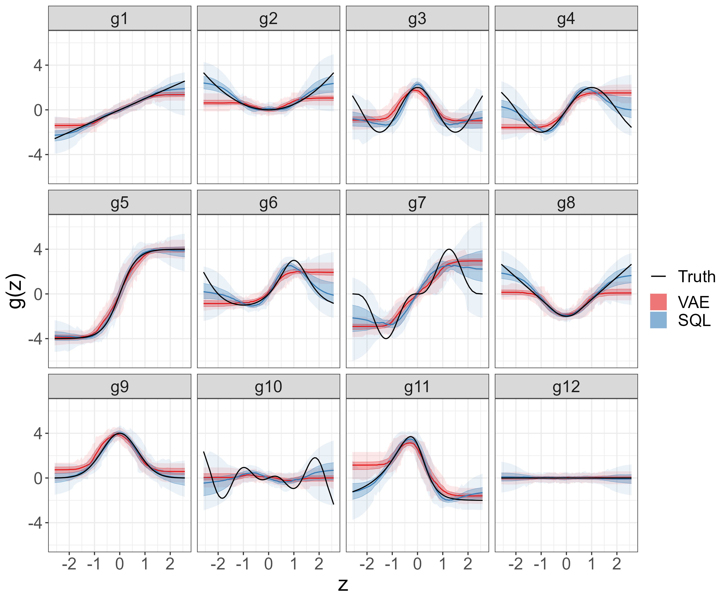
Figure 1: Functional boxplot of the $12$ functions composing the generator (Model M1) when $n=100$. The black line represents the ground truth. The estimated functions of SQL are in blue. The estimated functions of the VAE are in red. We see that, across all 12 variables, the estimated functions using SQL are closer to the ground truth than those estimated by the VAE. This is observed for cases when the ground truth is linear ($g_{1}$ and $g_{12}$), polynomial ($g_{2}$), trigonomotric ($g_{3},g_{4}$, and $g_{5}$), and complex functions.

4.1 Simulation design

We focus on two sets of common and general scenarios, low-dimensional and high-dimensional data, to investigate the properties of the estimators. In Model M1, we investigate if SQL can challenge VAE in a classical setting, that is, with a (very) low-dimensional model, with a small number of selected generators. In this scenario, we focus on one factor and we let the sample size vary. In Model M2, we study an increasingly common type of data, that is, high-dimensional data, and investigate the impact of increasing dimensionality on the performance of the competing methods when the sample size is fixed. In this setting, we used randomly generated smooth functions to obtain the generator.

Table 1: Summary of the performance of the estimators in Model M1 ($p=12$). We report both the median and median absolute deviations (in parentheses) over the $100$ Monte Carlo runs.

$n$	SQL		VAE
	$\text{mse}_{z}$	$\text{mse}_{g}$	$\text{mse}_{z}$	$\text{mse}_{g}$
50	0.112 (0.071)	0.46 (0.18)	0.132 (0.057)	0.516 (0.126)
100	0.095 (0.053)	0.277 (0.1)	0.118 (0.05)	0.402 (0.106)
500	0.053 (0.015)	0.087 (0.025)	0.059 (0.039)	0.172 (0.062)
1000	0.048 (0.009)	0.059 (0.017)	0.027 (0.004)	0.079 (0.015)

Model M1 (Low dimensionality).

We consider a framewwork with $q=1$ factor and $p=12$ variables, and we let $n\in\{50,100,500,1000\}$. The $12$ functions are generated by

$$f_{1}(Z) =Z,\quad\qquad f_{2}(Z) =Z^{2}/2,$$

$$f_{3}(Z) =2\cos(\pi Z/1.5),\quad f_{4}(Z) =2\sin(0.5\pi Z),$$

$$f_{5}(Z) =4\tanh(1.5Z),\quad f_{6}(Z) =\frac{3\sin(0.5\pi Z)}{(2-\sin(0.5\pi Z))},$$

$$f_{7}(Z) =4\sin(0.4\pi Z)^{3},\quad f_{8}(Z) =4J(Z)-2,$$

$$f_{9}(Z) =4\exp(-Z^{2}), f_{10}(Z) =Z\cos(3.5Z),$$

$$f_{11}(Z) =\frac{10\exp(Z)}{(1+\exp\{4Z\})}-2, f_{12}(Z) =0,$$

where $J(Z)=0.5\left(Z^{2}\mathbbm{1}(|Z|<0.5)+(|Z|-0.25)\mathbbm{1}(|Z|\geq 0.5)\right)$ is the Huber function with parameter $0.5$. Both the factors and the errors are generated as independent $\mathcal{N}(0,1)$.

We present the results of the simulation study of Model M1 in Figure 1 and Table 1.

Model M2 (Large dimensionality).

We consider a framework where $n=200$ and $p\in\{20,50,100,200,500\}$ and we consider $q\in\{1,3\}$ latent factors. To simulate the large number of functions, we generate them randomly using trigonometric functions. Specifically, we generate

$$\tilde{f}_{j,l}(Z)=\frac{1}{C_{j,l}}\sum_{m=1}^{4}\alpha_{j,l,m}\cos(2\pi mZ/8)+\beta_{j,l,m}\sin(2\pi mZ/8),$$

where $\alpha_{j,l,m}$ and $\beta_{j,l,m}$ are both independently generated from $\mathcal{N}(0,m^{-2})$ for $j=1,...,p$, and $C_{j,l}$ are rescaling constants, where $C_{j,l}=\sum_{m=1}^{4}\alpha_{j,l,m}^{2}+\beta_{j,l,m}^{2}$. We then recenter the random functions, as

$$f_{j,l}(Z)=\tilde{f}_{j,l}(Z)-\mathbb{E}[\tilde{f}_{j,l}(Z)]$$

to ensure identifiability. The factors $Z_{{i,l}}$ are generated as independent $\mathcal{N}(0,1)$ and the errors $\epsilon_{i,j}$ as $\mathcal{N}(0,1.5^{2})$.

We present the simulation results of Model M2 in Table 2.

4.2 Implementation

To implement SQL, we use normalized B-splines (Schumaker,, 2007). Given $M+4$ evenly distributed knots, we obtain $M$ B-splines basis functions of order $3$, denoted as $\{\tilde{\Psi}_{1},\tilde{\Psi}_{2},...,\tilde{\Psi}_{M}\}$. As in Boente and Martínez, (2023), we center the B-splines functions in order to guarantee that the estimated functions are also centered. We thus define $\Psi_{k}(u)=\tilde{\Psi}_{k}(u)-\int_{0}^{1}\tilde{\Psi}_{k}(u)du$ and use only the first $d=M-1$ basis functions to ensure that they are linearly independent. We select $d=10$ for Model M1 and $d=8$ for Model M2, respectively. Further, we select the tuning parameter $\lambda$ using generalized cross-validation over a grid of length $20$. We provide the details of the numerical implementation for the VAE in the Appendix C.

Table 2: Summary of the performance of the estimators in Model M2 ($n=200$). We report both the median and median absolute deviations (in parentheses) over the $100$ Monte Carlo runs.

	$p$	SQL		VAE
		$mse_{z}$	$mse_{f}$	$mse_{z}$	$mse_{f}$
$q=1$	20	0.922 (0.294)	0.466 (0.126)	0.866 (0.242)	0.278 (0.104)
	50	0.34 (0.167)	0.205 (0.052)	0.512 (0.206)	0.25 (0.067)
	100	0.11 (0.038)	0.092 (0.021)	0.245 (0.119)	0.169 (0.034)
	200	0.049 (0.012)	0.061 (0.005)	0.105 (0.046)	0.131 (0.020)
	500	0.033 (0.010)	0.056 (0.004)	0.102 (0.031)	0.135 (0.014)
$q=3$	20	1.003 (0.119)	0.6 (0.056)	0.924 (0.127)	0.274 (0.049)
	50	0.846 (0.195)	0.279 (0.048)	0.937 (0.211)	0.225 (0.039)
	100	0.433 (0.328)	0.136 (0.083)	0.796 (0.212)	0.182 (0.037)
	200	0.059 (0.026)	0.065 (0.005)	0.748 (0.276)	0.174 (0.047)
	500	0.031 (0.006)	0.056 (0.001)	0.723 (0.257)	0.19 (0.057)

4.3 Simulation results

For each set of parameters, we conduct 100 Monte Carlo experiments. To evaluate the prediction performance of the estimation methods, we report the mean squared error of the factors, given by

$$\text{mse}_{z}=\frac{1}{qn}\sum_{i=1}^{n}\sum_{l=1}^{q}\left(\hat{Z}_{i,l}-Z_{i,l}\right)^{2},$$

as well as the mean squared prediction error of the generator, given by

$$\text{mse}_{f}=\frac{1}{qp}\sum_{j=1}^{p}\sum_{l=1}^{q}\mathbb{E}\left[\left(\hat{f}_{j,l}(Z)-f_{j,l}(Z)\right)^{2}\right].$$

The above expectation is approximated by a sample of $1000$ points from the standard normal distribution.

In the classical setting of Model M1, with $p$ fixed and small, the accuracy of both methods improve as $n$ increases. SQL outperforms VAE for $n=50,100$, and $500$. For $n=1000$, however, the mean square error $\text{mse}_{z}$ is lower for VAE, while $\text{mse}_{f}$ is lower for SQL. Figure 1 depicts the estimated functions for both methods when $n=100$. We can see that the SQL exceeds the VAE, especially on the tails.

In Model M2, where $n$ is fixed, the performance of SQL improves significantly as $p$ increased. For VAE, there is a slight trend of improvement observed. SQL outperforms VAE when $p\geq 50$ for $q=1$ and when $p\geq 100$ for $q=3$. These simulations suggest three messages. (1) In settings with small sample sizes and small dimensionality, SQL has a modest advantage over VAE. (2) In settings with large sample sizes and small dimensionality, SQL can compete with VAE. (3) When the dimensionality is larger, SQL has a significant advantage, and the advantage becomes increasingly obvious as the dimensionality grows. These findings confirms empirically the rates of convergence which states that the performance of SQL depends on $\log(n)/p$.

5 Application to gene expression data

After presenting the theory and methods and evaluating them via simulation studies, in this section, we apply the SQL method to gene expression data of cancer patients. Many types of cancer have a genetic basis. The studies of the links between genes and oncological outcomes may not only help finding potential new genetic underpinings of specific cancer types but also help predicting the disease outcomes. Indeed, gene expression data have been used to classify cancer (Golub et al.,, 1999). Yet, despite advances, most cancer classifications rely on linear explorations. While linear methods are simple and easy to explain, this may naturally leave out a vast territory where genetic variables nonlinearly affect the outcomes. Additionally, when the dimensionality of genetic data is high, linear dimensional reduction may fail to uncover lower-dimensional representations whose relationship with the outcomes is non-linear. This problem may be further exacerbated when the lower-dimensional representations are used as features (predictors), as they perhaps only explain the portion of total disease variability that is linearly relevant.

The proposed SQL framework provides a platform to identify and estimate the lower-dimensional factors that are both linearly and nonlinearly related with, and therefore, better predict and potentially better explain, the outcomes. In this paper, we apply SQL to investigate the RNA-Seq dataset from the Pan-Cancer Atlas (PanCanAtlas) Initiative. In brief, the PanCanAtlas data contain gene expressions ($p=20,263$ genes with non-null expressions) from $801$ patients. Five types of tumors are present among these patients: breast cancer ($n=300$), kidney cancer ($n=146$), colon cancer ($n=78$), lung cancer ($n=141$), and prostate cancer ($n=136$). See http://archive.ics.uci.edu/ml for detailed information about the dataset.

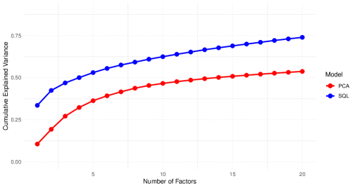
Figure 2: Proportion of the explained variance among total variance of the gene expression data with $p=20263$ genes. SQL explains $42.4\%$ of the variance with $2$ factors compared to $19.3\%$ by PCA. To explain $50\%$ of the variance, SQL requires only $4$ factors, while PCA requires $14$ components.

We use SQL to perform cancer genetic data analysis in three domains: unsupervised learning, supervised learning, and latent space explainable analysis.

First, we apply SQL to study the data in an unsupervised manner to (a) find nonlinear latent factors that explain important variability of the total data; and (b) discover cancer-specific latent factors that separate cancer categories. We carry out SQL analysis vis-à-vis principal component analyis (PCA), a prominent linear competitor. Specifically, we begin by re-scaling the gene expression data. Then, consistent to the steps in the simulation study, we used normalized cubic B-splines bases, with $d=12$. We choose the Gaussian CDF as $P_{Z}$ and select the tuning parameter using generalized cross-validation. To select the number of factors, we use

$$EV(q)=1-\frac{\sum_{i=1}^{n}\sum_{j=1}^{p}(X_{i,j}-\sum_{l=1}^{q}\hat{f}_{j,l}(\hat{Z}_{i,l}))^{2}}{\sum_{i=1}^{n}\sum_{j=1}^{p}X_{i,j}^{2}},$$ (12)

where the measure $EV(q)$ may be regarded as the proportion of the total variation explained by the model. Finally, we fit SQL for $q=1,2,...,20$, compute the proportion of explained variance, and compare it with the explained variance of PCA in Figure 2. Our results suggest that, compared to PCA, SQL is able to explain the variance with fewer factors. In particular, with $2$ factors, SQL explains $42.4\%$ of the variance compared to $19.3\%$ by PCA. To explain $50\%$ of the variance, SQL needs only $4$ factors, while PCA needs $14$ factors.

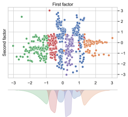
(a) SQL

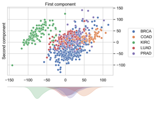
(b) PCA

Figure 3: Visualization of the two-dimensional latent space of the 20,263 genes from $801$ patients. The embedding plots suggest that SQL yields a better separation of five cancer types along its first factor (Panel a) compared to PCA along its first component (Panel b). The improved separation via SQL is further illustrated by the conditional density estimates depicted at the bottom of each plot. The colour codes for the dots and histograms are blue = breast cancer (BRCA), yellow = colon cancer (COAD), green = kidney cancer (KIRC), red = lung cancer (LUAD), and purple = prostate cancer (PRAD).

Second, we use the identified latent features to classify cancer types using supervised learning. To that end, we feed the first two latent factors from SQL into the Support Vector Machine (SVM) to classify five cancer types. To avoid a chance fitting (a good fit due to a lucky training/test split), we implement repeated random sub-sampling validation, with test sets of size $160$ and $100$ random sub samples. This yields a mean accuracy of $97.16\%$ (sd$=1.32$) for SQL, compared to $69.87\%$ (sd$=3.12$) using PCA. Next, we enquire into the potential reason why SQL outperforms PCA. To do so, we plot the first two factors against each other for SQL and PCA, respectively, in Figure 3. We can see that, graphically, SQL yields better (nonlinear) separation of five cancer types compared to PCA. This suggests that SQL is able to capture the nonlinearity in the data while PCA does not do as well.

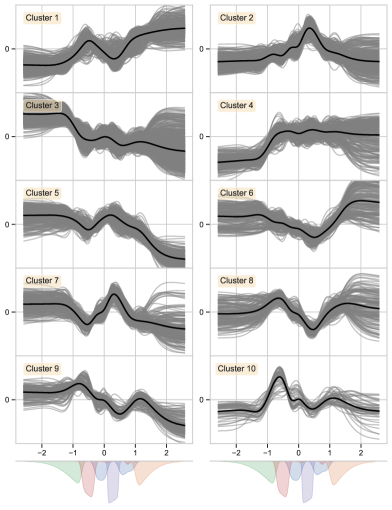
Figure 4: Visualization of $3,000$ generators that best explain the data via $10$ functional clusters. To help interpretation, we align the histograms of the factor for each cancer type on the x-axis. The colour codes for the histograms are blue = breast cancer (BRCA), yellow = colon cancer (COAD), green = kidney cancer (KIRC), red = lung cancer (LUAD), and purple = prostate cancer (PRAD). The results show that genes corresponding to functional cluster 4, for example, play a significant role in discriminating kidney cancer.

Lastly, we investigate the relationship between the first extracted latent factor and the gene expression features. As visualizing $20,263$ functions is difficult and potentially not meaningful, we first rank the functions and then select the top functions that best explain the data. One effective way to rank the functions are sorting them according to their norms $\|g\|_{\varphi}^{2}=\int_{-\infty}^{\infty}g(z)^{2}\varphi(Z)dz$, where $\varphi$ is the Gaussian density. We then select the top $3,000$ functions with the highest norms and fine-groom them using hierarchical clustering with distance metric $d(g_{1},g_{2})=\|g_{1}-g_{2}\|_{\varphi}$. This yields $10$ clusters, as plotted in Figure 4. In order to explore how genes relate to the cancer types via these functions, we add histograms of the factors for each cancer type along the x-axis, with which one can better interprete the clusters. For example, genes corresponding to functional cluster 4 play a significant role in discriminating kidney cancer from other cancer types. For genetic pathologists, it may be of further interest to explore the roles of the genes in each cluster and how they may give rise to the oncological outcomes via individual clusters using, for example, functional pathway analysis. This is, however, beyond the scope of the present paper and we will leave it to future work.

Taken together, using high-dimensional genetic data from patients of five types of cancer, we show that the SQL method is able to uncover group-specific factors that not only better separate the groups but also explain a larger amount of variability than their linear counterparts. Additionally, using the latent factors as predictors, SQL is able to yield better out-of-sample prediction performance (than linear competitors) to classify cancer types in previously unseen subjects. Finally, the latent factors, as well as their associated functional clusters, help deliver meaningful scientific interpretation regarding the lower-dimensional representations and potentially identify and isolate functional genetic clusters related to cancerous outcomes.

6 Conclusions

In this paper, we introduce a new statistical method, Statistical Quantile Learning (SQL), to study large-scale nonlinear high-dimensional data. Methodologically, by using a quantile approximation, SQL incorporates the characteristics of nonparametric statistics and constitute an alternative to deep generative models, overcoming some of their limitations. Compared to nonlinear factor models, SQL flexibly takes advantage of the rich nonparametric space. Theoretically, SQL is identifiable and the rates of convergence improve as both the sample size and feature dimensionality increase. Empirically, our simulations suggest that SQL competes with VAE in settings with relatively large sample sizes, and has a significant advantage in large and high dimensional settings. Additionally, a study of high-dimensional gene expression data from cancer patients shows that SQL extends even to supervised learning: the extracted latent factors, predictive of five types of cancer, can potentially serve as biomarkers.

There are a few directions this paper has not explored. First, we consider additive functions for the generator because it avoids the curse of dimensionality and provides more avenues for interpretability. However, this omits the scenarios where the generator is a multivariate function of the factors. Future work may investigate this and extend our framework to multivariate generators. Second, further research may also explore and enhance our algorithm. As the Quadratic Assignment Problem can be solved exactly in polynomial time in certain specific cases, a key area of future work may be the selection of an appropriate functional space, or sieve space, which has the potential to lead to more efficient computational algorithms. Third, while nonparametric inference offers flexibility, it is contingent on certain assumptions that may not always be fulfilled in real applications, and it is often notably impacted by the presence of a small number of outliers. This may affect the accuracy of the estimator but also the efficiency of the algorithm. One way to deal with this issue is to couple SQL with robust statistical methods (see e.g. Hampel et al., (2011), Ronchetti and Huber, (2009), and Maronna et al., (2019) ), which are designed to provide stable inference when slight deviations from the stochastic assumptions on the model occur. Robustification of the SQL approach may be achieved using robust sieve M-estimators, as in Bodelet and La Vecchia, (2022). Additionally, we conjecture that combining our results with Lemma 1 in Bodelet and La Vecchia, (2022) may give similar rates of convergence for the robustified SQL estimates.

To summarize, in the present study, we propose SQL, a large, nonlinear, and additive model suitable for the analysis of nonlinear high-dimensional data. The method leverages the flexibility of nonparametric statistics. Its theoretical properties allow one to quantify and assess the model performance given different sample sizes and feature dimensionality. Its applications to high-dimensional genetic data suggest its utility in both unsupervised learning (e.g., separating samples from different groups) and supervised learning (e.g., extracting latent features to predict disease outcomes). The enclosed SQL package (https://github.com/jbodelet/SQL) helps users to further explore and test the method and theory in a broad range of applications to investigate the nonlinear patterns of high-dimensional brain imaging data, gene expression data, and whole-body immunological biomarkers.

Appendix A Proofs for the asymptotic theory

A.1 Notation

We define $a\vee b=\max(a,b)$ and $a\wedge b=\min(a,b)$. Throughout the proofs, we let $C$ be a generic absolute constant, whose value may change from line to line. For two sequences $\alpha_{n}$ and $\beta_{n}$, we use $\alpha_{n}=o(\beta_{n})$ to denote $\alpha_{n}/\beta_{n}\rightarrow 0$ and $\alpha_{n}=\mathcal{O}(\beta_{n})$ to denote $\alpha_{n}\leq C\beta_{n}$ for all $n$ large enough. Moreover, for a random sequence $X_{n}$, we use $X_{n}=o_{p}(a_{n})$ to denote $X_{n}/a_{n}\rightarrow 0$ in probability, and $X_{n}=\mathcal{O}_{p}(a_{n})$ if $\lim_{M\rightarrow\infty}\limsup_{n\rightarrow\infty}P(|X_{n}|>M\alpha_{n})=0$.

A.2 Entropy lemma

Before considering the rates of convergence, we first provide a general bound on the entropy of the parameter space. Given a space $\mathcal{G}_{n}$ and the space of permutations $\Pi_{n}$, we build the following space

$$\mathcal{H}_{n}:=\left\{h:\{1,\dots,n\}\times\{1,\dots,p\}\rightarrow\mathbb{R},h_{{i,j}}=\sum_{l=1}^{q}g_{j,l}\left(\frac{\pi^{(l)}_{i}}{n+1}\right),g_{1},\dots,g_{p}\in\mathcal{G}_{n}^{\oplus q},\pi^{(1)},\dots,\pi^{(q)}\in\Pi_{n}\right\}.$$

We consider the norm $\|h\|^{2}:=\frac{1}{np}\sum_{j=1}^{p}\sum_{i=1}^{n}h_{i,j}^{2}$. The penalized estimator $\hat{h}$ can be then expressed as

$$\hat{h}\in\operatorname*{arg\,min}_{h\in\mathcal{H}_{n}}\|X-h\|^{2}+\lambda I^{2}(h)$$

where for $h_{i,j}=\sum_{l=1}^{q}g_{j,l}(\frac{\pi^{(l)}}{n+1})$ we define with a slight abuse of notation

$$I^{2}(h):=I^{2}(\bm{g})=\frac{1}{p}\sum_{j=1}^{p}\sum_{l=1}^{q}\int_{0}^{1}|g_{j,l}^{(m)}(\xi)|^{2}d\xi.$$

We will also denote the true solution by $h^{0}_{i,j}:=\sum_{l=1}^{q}g_{j,l}^{0}(Z_{i,l}^{0})$ that satisfies

$$X_{i,j}=h^{0}(i,j)+\epsilon_{i,j}.$$

Note that $h^{0}$ may not belong to $\mathcal{H}_{n}$. We then define

$$h_{n}^{*}\in\operatorname*{arg\,min}_{h\in\mathcal{H}_{n}}\|h-h^{0}\|^{2}+\lambda I^{2}(h),$$

where $h_{n}^{*}$ can be interpreted as the “closest” element in $\mathcal{H}_{n}$ to $h^{0}$. We also denote by $\bm{g}^{*}$ and $\bm{\pi}^{*}$ the functions and permutation vector that satisfy $h^{*}_{i,j}=\sum_{l=1}^{q}g^{*}_{j,l}(\frac{\pi^{*(l)}}{n+1})$.

We also define, for any $\delta>0$, the family of sets

$$\mathcal{H}_{n}(\delta):=\{h\in\mathcal{H}_{n},\;\|h-h^{*}\|^{2}+\lambda I^{2}(h)\leq\delta^{2}\}.$$

Moreover, for $g\in\mathcal{G}_{n}^{\oplus q}$, we let the empirical norm be

$$\|g\|_{n}^{2}:=\frac{1}{n}\sum_{i=1}^{n}\sum_{l=1}^{q}\left(g_{j,l}\left(\frac{i}{n+1}\right)\right)^{2},$$

and we define, for any $\delta>0$, the family of sets

$$\mathcal{G}_{n}^{\oplus q}(\delta):=\{g\in\mathcal{G}_{n}^{\oplus q},\;\|g-g^{*}\|^{2}_{n}+\lambda I^{2}(g)\leq\delta^{2}\}.$$

For a set $\mathcal{S}$ and norm $\|\cdot\|$, we define the covering number $N(\varepsilon,S,\|\cdot\|)$ to be the smallest number of balls of radius $\delta$ to cover $\mathcal{S}$. We call $H(\varepsilon,S,\|\cdot\|):=\log N(\varepsilon,S,\|\cdot\|)$ the entropy of $\mathcal{S}$ and we define the entropy integral as

$$J(\delta,S,\|\cdot\|)=\int_{0}^{\delta}H^{1/2}(\varepsilon,\mathcal{S},\|\cdot\|)d\varepsilon,$$

provided it exists.

The following lemma states that the metric entropy of $\mathcal{H}_{n}(\delta)$ can be computed from the metric entropy of $\mathcal{G}_{n}(\delta)$.

Lemma 2.

Let Assumption A1 and A2 be satisfied and suppose that, for any $\varepsilon>0$ we have $N(\varepsilon,\mathcal{G}_{n}(\delta/q),\|\cdot\|_{n})<\infty$. We have for some $C>0$ that

$$H(\varepsilon,\mathcal{H}_{n}(\delta),\|\cdot\|)\leq q\log(n!)+pqH(\varepsilon,\mathcal{G}_{n}(\delta/q),\|\cdot\|_{n})$$

for all $\varepsilon>0$ and any $\lambda\geq 0$. Moreover, we have

$$J(\delta,\mathcal{H}_{n}(\delta),\|\cdot\|)\leq\sqrt{q\log(n!)}\delta+\sqrt{pq}J(\delta,\mathcal{G}_{n}(\delta/q),\|\cdot\|_{n}).$$

A.3 Proof of Lemma 1

First, define $(\bm{g}^{*},\bm{\pi}^{*})$ as minimizers of

$$\frac{1}{{np}}\sum_{i=1}^{n}\sum_{j=1}^{p}\left(\sum_{l=1}^{q}g_{j,l}\left(\frac{\pi_{i}^{(l)}}{n+1}\right)-f_{j,l}^{0}({\bm{Z}}_{i}^{0})\right)^{2}+\lambda I^{2}(\bm{g}).$$

Using the inequality $(a+b)^{2}\leq 2a^{2}+2b^{2}$ we obtain

$$\frac{1}{{np}}\sum_{i=1}^{n}\sum_{j=1}^{p}\left(\sum_{l=1}^{q}g_{j,l}^{*}\left(\frac{\pi_{i}^{*(l)}}{n+1}\right)-f_{j,l}^{0}({\bm{Z}}_{i}^{0})\right)^{2}+\lambda I^{2}(\bm{g}^{*})$$

$$\leq\min_{g_{j}\in\mathcal{G}_{n}^{\oplus q}}\min_{\pi^{(l)}\in\Pi_{n}}\frac{1}{{np}}\sum_{i=1}^{n}\sum_{j=1}^{p}\bigg{(}\sum_{l=1}^{q}g_{j,l}^{*}\left(\frac{\pi_{i}^{*(l)}}{n+1}\right)-f_{j,l}\circ P_{Z}^{-1}\left(\frac{\pi_{i}^{(l)}}{n+1}\right)+f_{j,l}\circ P_{Z}^{-1}\left(\frac{\pi_{i}^{(l)}}{n+1}\right)-f_{j,l}^{0}({\bm{Z}}_{i}^{0})\Bigg{)}^{2}+\lambda I^{2}(\bm{g})$$

$$\leq\min_{g_{j}\in\mathcal{G}_{n}^{\oplus q}}\frac{2}{{np}}\sum_{i=1}^{n}\sum_{j=1}^{p}\left(\sum_{l=1}^{q}g_{j,l}\left(\frac{\pi_{i}^{(l)}}{n+1}\right)-f_{j,l}\circ P_{Z}^{-1}\left(\frac{\pi_{i}^{(l)}}{n+1}\right)\right)^{2}+\lambda I^{2}(\bm{g})+$$

$$\min_{\pi^{(l)}\in\Pi_{n}}\frac{2}{{np}}\sum_{i=1}^{n}\sum_{j=1}^{p}\left(\sum_{l=1}^{q}f_{j,l}^{0}\circ P_{Z}^{-1}\left(\frac{\pi^{(l)}_{i}}{n+1}\right)-f_{j,l}^{0}(Z_{i,l}^{0})\right)^{2}.$$

For the first component, we obtain

$$\min_{g_{j}\in\mathcal{G}_{n}^{\oplus q}}\frac{2}{{np}}\sum_{i=1}^{n}\sum_{j=1}^{p}\left(\sum_{l=1}^{q}g_{j,l}\left(\frac{\pi_{i}^{(l)}}{n+1}\right)-f_{j,l}\circ P_{Z}^{-1}\left(\frac{\pi_{i}^{(l)}}{n+1}\right)\right)^{2}+\lambda I^{2}(\bm{g})\leq 2\tau_{n}^{*}$$

where

$$\tau_{n}^{*}=\min_{g_{j}\in\mathcal{G}_{n}^{\oplus q}}\frac{1}{{np}}\sum_{i=1}^{n}\sum_{j=1}^{p}\sum_{l=1}^{q}\left(g_{j,l}\left(\xi_{i}\right)-f_{j,l}\circ P_{Z}^{-1}\left(\xi_{i}\right)\right)^{2}+\lambda I^{2}(\bm{g})$$

For the second component, we apply Assumption A2 to get that, for any $Z_{i,l}$,

$$\frac{2}{{np}}\sum_{i=1}^{n}\sum_{j=1}^{p}\left(\sum_{l=1}^{q}f_{{j,l}}^{0}\left(\frac{\pi^{(l)}_{i}}{n+1}\right)-f_{{j,l}}^{0}(Z_{i,l}^{0})\right)^{2} \leq\frac{2q}{{np}}\sum_{i=1}^{n}\sum_{j=1}^{p}\sum_{l=1}^{q}\left(f_{{j,l}}^{0}\left(\frac{\pi^{(l)}_{i}}{n+1}\right)-f^{0}_{{j,l}}(Z_{i,l}^{0})\right)^{2}$$

$$\leq\frac{2L_{n}^{2}q}{n}\sum_{i=1}^{n}\sum_{l=1}^{q}\left(P_{Z}^{-1}\left(\frac{\pi^{(l)}_{i}}{n+1}\right)-Z_{i,l}^{0}\right)^{2}.$$

Now we will show that, when taking the minimum over $\bm{\pi}$, the right hand side of the above inequality converges with rate $n^{-1}$. Denote the $k$-th order statistics by $Z^{0}_{(k),l}$, so we have $Z^{0}_{(1),l}\leq Z^{0}_{(2),l}\leq\dots\leq Z^{0}_{(n),l}$. Note that we can write:

$$\min_{\pi^{(l)}}\frac{1}{n}\sum_{i=1}^{n}\left(P_{Z}^{-1}\left(\frac{\pi^{(l)}_{i}}{n+1}\right)-Z_{i,l}^{0}\right)^{2}=\frac{1}{n}\sum_{i=1}^{n}\left(P_{Z}^{-1}\left(\frac{i}{n+1}\right)-Z_{(i),l}^{0}\right)^{2}.$$

Denote by $P_{n}^{(l)}(z):=\frac{1}{n+1}\sum_{i=1}^{n}\mathbbm{1}(Z_{{i,l}}\leq z)$ the empirical distribution of the $l$-th factors, and by $P^{(l)-1}_{n,l}(p):=\inf\{z:P_{n}^{(l)}(z)\geq p\}$ the corresponding empirical quantile function. Given Assumption A1, we can use the results in Lemma 21.4 and Corollary 21.5 in Van der Vaart, (2000) which shows that the empirical quantile function converges to the theoretical quantile function with the same rate of converge as the cumulative distribution function. In particular, we have, for any $\xi\in(0,1)$, that

$$\sqrt{n}\left(P_{n}^{(l)-1}(\xi)-P^{-1}_{Z}(\xi)\right)=\frac{-1}{\sqrt{n}}\sum_{i=1}^{n}\frac{\mathbbm{1}(Z_{{i,l}}\leq P_{Z}^{-1}(\xi))-P_{Z}(\xi)}{p_{Z}^{(l)}(P_{Z}^{-1}(\xi))}+o_{p}(1).$$

As we have $Z_{(i),l}^{0}=P_{n}^{(l)-1}(\frac{i}{n+1})$, we can apply the egodic property in Assumption A1 to obtain for some constant $K>0$ that

$$\min_{\pi^{(l)}}\frac{1}{n}\sum_{i=1}^{n}\left(\frac{\pi_{i}^{(l)}}{n+1}-Z_{i,l}^{0}\right)^{2}\leq K\sup_{z}\left|P_{n}^{(l)}(z)-P_{Z}(z)\right|^{2}+o_{p}\left(\frac{1}{n}\right)=O_{p}\left(\frac{1}{n}\right).$$

Combining the above results gives

$$\min_{g_{j}\in\mathcal{G}^{\oplus q},\pi^{(l)}\in\Pi_{n}}\frac{1}{{np}}\sum_{i=1}^{n}\sum_{j=1}^{p}\left(\sum_{l=1}^{q}g_{j,l}\left(\frac{\pi_{i}^{(l)}}{n+1}\right)-f_{j,l}^{0}(Z_{i,l}^{0})\right)^{2}=\mathcal{O}_{p}\left(\tau_{n}^{*}+\frac{L_{n}^{2}}{n}\right).$$

A.4 Proof of Lemma 2

Let $\mathcal{C}_{g}:=\{g^{1},\dots,g^{N}\}$ denotes the $\varepsilon$-covering of $\mathcal{G}^{\oplus q}(\delta)$ with $N=N(\varepsilon,\mathcal{G}^{\oplus q}(\delta),\|\cdot\|_{n})$. Let’s choose $\tilde{h}\in\mathcal{H}_{n}(\delta)$, defined by $\tilde{h}(i,j)=\sum_{l=1}^{q}\tilde{g}_{j,l}\left(\frac{\tilde{\pi}^{(l)}}{n+1}\right)$ where $\tilde{g}_{j}\in\mathcal{G}^{\oplus q}(\delta)$. There are $k_{1},\dots,k_{p}$ such that $g^{k_{j}}\in\mathcal{C}_{g}$ with $\|\tilde{g}_{j}-g^{k_{j}}\|_{n}\leq\varepsilon$. We can then build $h$ that satisfies $h(i,j)=\sum_{l=1}^{q}g_{l}^{k_{j}}\left(\frac{\tilde{\pi}^{(l)}}{n+1}\right)$. Obvisously we have $\|\tilde{h}-h\|\leq\sqrt{\frac{1}{p}\sum_{j=1}^{p}\|\tilde{g}_{j}-g^{k_{j}}\|^{2}_{n}}\leq\varepsilon$. The set

$$\mathcal{C}_{h}=\left\{h,h(i,j)=\sum_{l=1}^{q}g_{l}^{k_{j}}\left(\frac{\pi^{(l)}_{i}}{n+1}\right),g^{k_{1}},\dots,g^{k_{p}}\in\mathcal{C}_{g},\pi^{(1)},\dots,\pi^{(q)}\in\Pi_{n}\right\}.$$

is thus an $\varepsilon$-covering of $\mathcal{H}_{n}(\delta)$ with respect to $\|\cdot\|$. Its cardinal $\mathcal{C}_{h}$ is given obviously by $(n!)^{q}N^{p}$. We conclude that

$$H(\varepsilon,\mathcal{H}_{n}(\delta),\|\cdot\|)=\log N(\varepsilon,\mathcal{H}_{n}(\delta),\|\cdot\|)\leq q\log(n!)+pH(\varepsilon,\mathcal{G}_{n}^{\oplus q}(\delta),\|\cdot\|_{n}).$$ (13)

Now we use Lemma 8 in Sadhanala and Tibshirani, (2019) which computes bounds on additive sets to get

$$H(\varepsilon,\mathcal{G}_{n}^{\oplus q}(\delta),\|\cdot\|_{n})\leq qH(\varepsilon,\mathcal{G}_{n}(\delta/q),\|\cdot\|_{n})$$

Taking the integral of the square root of the right hand side of (13) gives a bound on Dudley’s integral:

$$J(\delta,\mathcal{H}_{n}(\delta),\|\cdot\|)\leq\sqrt{q\log(n!)}\delta+\sqrt{pq}J(\delta,\mathcal{G}(\delta),\|\cdot\|_{n}).$$

A.5 Proof of Theorem 1

The total error is separated into an approximation and the estimation error. Using $g_{j}^{*}$ and $\pi^{*}$ in Lemma 1, we decompose the total error into an estimation error and an approximation error as follows:

$$\sqrt{\frac{1}{{np}}\sum_{i=1}^{n}\sum_{j=1}^{p}\left(\hat{f}_{j}(\hat{\bm{Z}}_{i})-f_{j}^{0}({\bm{Z}}_{i}^{0})\right)^{2}} \leq$$

$$\underbrace{\sqrt{\frac{1}{{np}}\sum_{i=1}^{n}\sum_{j=1}^{p}\left(\sum_{l=1}^{q}\hat{f}_{j,l}(\hat{Z}_{i,l})-g_{j,l}^{*}\left(\frac{\pi_{i}^{*(l)}}{n+1}\right)\right)^{2}}}_{\text{estimation error}} +\underbrace{\sqrt{\frac{1}{{np}}\sum_{i=1}^{n}\sum_{j=1}^{p}\left(\sum_{l=1}^{q}g_{j,l}^{*}\left(\frac{\pi_{i}^{*(l)}}{n+1}\right)-f_{j,l}^{0}(Z_{i,l}^{0})\right)^{2}}}_{\text{approximation error}}.$$

The approximation error is bounded using Lemma 1. From Assumption A4 we have

$$\tau^{*}_{n}=\mathcal{O}(d^{-2\eta}).$$ (14)

Now we just need a bound for the estimation error. Let $\Psi(\delta)\geq J(\delta,\mathcal{H}_{n}(\delta),\|\cdot\|)$ be such that $\Psi(\delta)/\delta^{2}$ is a decreasing function of $\delta$. Applying Theorem 10.11 in van de Geer, 2000b , which treats rates of convergence for least squares estimators on sieves, for some $c$ depending on $K$ and $\sigma$ and for $\delta_{np}$ satisfying

$$\sqrt{np}\delta_{np}^{2}\geq c\Psi(\delta_{np}),\quad\text{ for all }n,$$ (15)

we have

$$\|\hat{h}-h^{*}\|=\mathcal{O}(\delta_{np}).$$ (16)

We use Lemma 2 to compute the entropy. The $\varepsilon$-covering number of $\mathcal{G}_{n}(\delta)$ can be bounded by

$$N(\varepsilon,\mathcal{G}_{n}(\delta/q),\|\cdot\|_{n})=\mathcal{O}\left(\left(\frac{4\delta/q+\varepsilon}{\varepsilon}\right)^{d}\right),$$

where we used Corollary 2.6 in van de Geer, 2000b , which states that the $\epsilon$-covering number for functions $g(\cdot)=\sum_{k=1}^{d}b_{k}\psi_{k}(\cdot)$ such that $\|\sum_{k=1}^{d}b_{k}\psi_{k}(\cdot)\|_{n}\leq M$ is of order $((4M+\varepsilon)/\varepsilon)^{d}$. We then get

$$H(\varepsilon,\mathcal{H}_{n}(\delta),\|\cdot\|)=\mathcal{O}\left(\log(n!)+pqd\log\left(\frac{4\delta/q+\varepsilon}{\varepsilon}\right)\right).$$ (17)

Integrating the square root of the entropy bound then yields

$$J(\delta,\mathcal{H}_{n}(\delta),\|\cdot\|) \leq C\delta\left[\sqrt{\log n!}+\sqrt{dp}\int_{0}^{1}\sqrt{\log(4/q+v)}dv\right],$$

$$\leq\tilde{C}\delta\left(\sqrt{\log n!}+\sqrt{dp}\right),$$

for some positive constants $C$ and $\tilde{C}$ which depend on $q$. Using inequality (15), it follows that (16) is satisfied for any $\delta_{np}$ such that, for some $\tilde{c}>0$,

$$\delta_{np}^{2}\geq\tilde{c}\left(\frac{\log n}{p}+\frac{d}{n}\right),$$

where Stirling formula gave $\log n!\asymp n\log n$. The theorem follows by combining (16) with Lemma 1 and (14).

A.6 Proof of Theorem 2

We first state the following lemma.

Lemma 3.

Suppose Assumptions A1, A2, and A3 are met. Take $\Psi(\delta)\geq J(\delta,\mathcal{H}_{n}^{*}(\delta),\|\cdot\|_{np})$ such that $\Psi(\delta)/\delta^{2}$ is a decreasing function of $\delta$, $0<\delta<2^{7}\sigma_{0}$. Then for

$$\sqrt{{np}}\delta_{np}^{2}=\Psi(\delta_{np}),\forall n,p$$

we have

$$\|\hat{h}-h^{0}\|^{2}+\lambda I^{2}(\hat{h})=\mathcal{O}_{p}\left(\delta_{np}^{2}+\|h^{*}-h^{0}\|^{2}+\lambda I^{2}(h^{*})\right).$$

The proof of Lemma 3 will be shown later. To conclude the theorem, we need to compute $\delta_{np}$ and the approximation error $\tau_{n}^{*}$.

We first compute the entropy for the penalized estimators. We use Lemma 2 and consider $\mathcal{G}_{n}=\mathcal{G}$ as the Sobolev space of $m$-th continuously differentiable functions. From Birman and Solomyak, (1967), we have that

$$H\left(\delta,\left\{g[0,1]\rightarrow\mathbb{R},\|g\|_{\infty}\leq 1,\int_{0}^{1}g^{(m)}(\xi)d\xi\leq 1\right\},\|\cdot\|_{\infty}\right)\leq C\delta^{-1/m},\quad\delta>0.$$

From this, following the same steps as in van de Geer, 2000a , we can show that

$$H(\delta,\mathcal{G}(\delta),\|\cdot\|_{n})\leq C\left(\delta^{1/m}\lambda^{-1/2m}\varepsilon^{-1/m}+\log\left(\frac{\delta}{(\sqrt{\lambda}\wedge 1)\varepsilon}\right)\right),\quad 0<\varepsilon<\delta,$$

which gives

$$J(\delta,\mathcal{G}(\delta),\|\cdot\|_{n})\leq\tilde{C}\left(\delta\lambda^{-1/2m}+\delta\sqrt{\log(1/\sqrt{\lambda}\vee 1)}\right),\forall\delta>0,$$

where $\tilde{C}$ depends on $m$. Using Lemma 2 we get

$$J(\delta,\mathcal{H}(\delta),\|\cdot\|)\leq C\delta\left(\sqrt{\log(n!)}+\sqrt{p}\lambda^{-1/2m}+\sqrt{p\log(1/\sqrt{\lambda}\vee 1)}\right),\forall\delta>0.$$

By Lemma 3 we can select $\delta_{np}$ satisfying

$$\sqrt{np}\delta_{n,p}\geq\left(\sqrt{\log(n!)}+\sqrt{p}\lambda^{-1/(2m)}+\sqrt{p\log(1/\sqrt{\lambda}\vee 1)}\right),$$

which gives

$$\delta_{n,p}^{2}\geq C\left(p^{-1}\log(n)+n^{-1}\lambda^{-1/(2m)}+n^{-1}\log(1/\sqrt{\lambda}\vee 1)\right).$$

Now we bound the approximation error. From Lemma 1 we have

$$\|h^{*}-h^{0}\|^{2}+\lambda I^{2}(h^{*})=\mathcal{O}_{p}\left(\frac{L_{n}^{2}}{n}+\tau_{n}^{*}\right).$$

We then use $\tau^{*}_{n}\leq\lambda I^{2}(\bm{g}^{0})$ to get

$$\|h^{*}-h^{0}\|^{2}+\lambda I^{2}(h^{*})=\mathcal{O}_{p}\left(\frac{L_{n}^{2}}{n}+\lambda I^{2}(\bm{g}^{0})\right).$$

Combining the bounds for the approximation and estimation errors concludes the proof.

A.7 Proof of Lemma 3

The estimator $\hat{h}$ satisfies

$$\|X-\hat{h}\|^{2}+\lambda I^{2}(\hat{h})\leq\|X-h^{*}\|^{2}+\lambda I^{2}(h^{*}),$$

and thus

$$\|\hat{h}-h^{0}\|^{2}+\lambda I^{2}(\hat{h})\leq 2\sup_{h\in\mathcal{H}_{n}}\langle\epsilon,\hat{h}-h^{*}\rangle+\|h^{*}-h^{0}\|^{2}+\lambda I^{2}(h^{*})$$

where we used the notation $\langle x,y\rangle=\frac{1}{np}\sum_{i=1}^{n}\sum_{j=1}^{p}x_{i,j}y_{i,j}$ for the empirical inner product. Moreover, we have

$$\|\hat{h}-h^{*}\|^{2}\leq 2\left(\|\hat{h}-h^{0}\|^{2}+\|h^{*}-h^{0}\|^{2}\right).$$

We then add $\lambda I^{2}(\hat{h})$ on both sides of the inequality to get

$$\|\hat{h}-h^{*}\|^{2}+\lambda I^{2}(\hat{h})\leq 2\|\hat{h}-h^{0}\|^{2}+2\|h^{*}-h^{0}\|^{2}+\lambda I^{2}(\hat{h})$$

and use the above supremum bound to get the basic inequality

$$\|\hat{h}-h^{*}\|^{2}+\lambda I^{2}(\hat{h})\leq 4\sup_{h\in\mathcal{H}_{n}}\langle\epsilon,\hat{h}-h^{*}\rangle+4\|h^{*}-h^{0}\|^{2}+2\lambda I^{2}(h^{*}).$$ (18)

On the set where $\langle\epsilon,\hat{h}-h^{*}\rangle<\|h^{*}-h^{0}\|^{2}+\lambda I^{2}(h^{*})$ the Lemma holds. On the set where $\langle\epsilon,\hat{h}-h^{*}\rangle\geq\|h^{*}-h^{0}\|^{2}+\lambda I^{2}(h^{*})$ we have

$$\|\hat{h}-h^{*}\|^{2}+\lambda I^{2}(\hat{h})\leq 8\sup_{h\in\mathcal{H}_{n}}\langle\epsilon,\hat{h}-h^{*}\rangle.$$

We can now apply the same arguments as in Theorem 9.1 in van de Geer, 2000b .

We then conclude by applying the triangle inequality $\|\hat{h}-h^{0}\|\leq\|\hat{h}-h^{*}\|+\|h^{*}-h^{0}\|$.

Appendix B Proof of Theorem 3

First we show that there exists an isomorphism $\bm{H}:\mathbb{R}^{q}\rightarrow\mathbb{R}^{q}$ such that ${\bm{Z}}=\bm{H}(\tilde{\bm{Z}})$. Assumption B2 implies that the Jacobian of $\bm{f}$ is full rank and hence $\bm{f}$ is injective. In particular, $\bm{f}$ is a diffeomorphism onto its image, $\bm{f}(\mathcal{Z}^{q})$. Then we show that $\tilde{\bm{f}}$ has to be a diffeomorphism on the same image $\bm{f}(\mathcal{Z}^{q})$. As a bijection (i.e., $\bm{f}$) exists between these two sets, they have same size. $\tilde{\bm{f}}$ has the same image and same support and thus must be a bijection too. Now for any $\bm{z}\in\mathbb{R}^{q}$, $\exists!\bm{x}\in\mathbb{R}^{p}$ such that $\bm{x}=\bm{f}(\bm{z})$. Then it exists a unique $\tilde{\bm{z}}\in\mathbb{R}^{q}$ such that $\bm{x}=\tilde{\bm{f}}(\tilde{\bm{z}})$. We then denote by $\bm{H}$ the invertible map that links this $\bm{z}$ to this $\tilde{\bm{z}}$. We have then

$$\tilde{\bm{\bm{f}}}(\tilde{\bm{Z}})=\bm{f}({\bm{Z}})=\bm{f}(\bm{H}(\tilde{\bm{Z}}))$$

and thus $\tilde{f}_{j}(\cdot)=f_{j}\circ\bm{H}(\cdot)$. Let $H_{1}(\cdot),...,H_{q}(\cdot)$ be the entries of $\bm{H}$. In order $\tilde{f}_{j}(\cdot)$ to satisfy Assumption B3 $\bm{H}$ has to be twice differentiable. Moreover, since $\tilde{f}_{j}$ are additive, it holds that for any $k^{\prime},k\in\{1,\ldots,q\}$ and $k^{\prime}\neq k$

$$\frac{\partial^{2}}{\partial z_{k}z_{k^{\prime}}}\tilde{g}_{j}(\bm{z})=0,\text{for }k\in\{1,\ldots,p\}$$

for any $\bm{z}=(z_{1},\ldots,z_{q})^{\top}\in\mathbb{R}^{q}$. Since $\tilde{f}_{j}=f_{j}\circ\bm{H}$, it yields, for any $k^{\prime}\neq k$, that

$$\sum_{l=1}^{q}g_{j,l}^{\prime}(H_{l}(\bm{z}))\frac{\partial^{2}H_{l}(\bm{z})}{\partial z_{k}\partial z_{k^{\prime}}}+g_{j,l}^{\prime\prime}(H_{l}(\bm{z}))\frac{\partial H_{l}(\bm{z})}{\partial z_{k}}\frac{\partial H_{l}(\bm{z})}{\partial z_{k^{\prime}}}=0,\text{for }j\in\{1,\ldots,p\}.$$ (19)

For any $\bm{z}\in\mathbb{R}^{q}$ and $k\neq j$, we thus have the linear systems of equations,

$$\bm{\Delta}(\bm{H}(\bm{z}))\bm{a}_{kk^{\prime}}(\bm{z})=0,$$

where $\bm{\Delta}(\bm{z})$ is the $p\times 2q$-dimensional matrix with rows $(f_{j1}^{\prime}(z_{1}),\ldots,f_{jq}^{\prime}(z_{q}),f_{j1}^{\prime\prime}(z_{1}),\ldots,f_{jq}^{\prime\prime}(z_{q}))$ and we define

$$\bm{a}_{kk^{\prime}}(z)=\left(\frac{\partial^{2}H_{1}(\bm{z})}{\partial z_{k}\partial z_{k^{\prime}}},\ldots,\frac{\partial^{2}H_{q}(\bm{z})}{\partial z_{k}\partial z_{k^{\prime}}},\frac{\partial H_{1}(\bm{z})}{\partial z_{k}}\frac{\partial H_{1}(\bm{z})}{\partial z_{k^{\prime}}},\ldots,\frac{\partial H_{p}(\bm{z})}{\partial z_{k}}\frac{\partial H_{p}(\bm{z})}{\partial z_{k^{\prime}}}\right)^{\top}.$$

We now apply Assumption B2 which specifies that $\bm{\Delta}(\bm{z})$ is full rank for any $\bm{z}\in\mathbb{R}^{q}$. This implies that there is only one unique solution $\bm{a}_{kk^{\prime}}(\bm{z})=0$ for any $k\neq k^{\prime}$ and thus

$$\frac{\partial^{2}H_{l}(\bm{z})}{\partial z_{k}\partial z_{k^{\prime}}}=0\quad\text{and}\quad\frac{\partial H_{l}(\bm{z})}{\partial z_{k}}\frac{\partial H_{l}(\bm{z})}{\partial z_{k^{\prime}}}=0,$$

for any $l\in\{1,\dots,q\}$. This implies that each entry $H_{l}(\bm{z})$ depends on at most one of the $z_{1},...,z_{q}$, i.e., each $H_{l}(\cdot)$ is a univariate function of one of the element of $(z_{1},\dots,z_{q})$. We can thus write by $H_{l}(\bm{z})=h_{l}(z_{\sigma(l)})$ for a univariate function $h_{l}$ and $\sigma_{l}\in\{1,\dots,q\}$ for $l\in\{1,\ldots,q\}$. We thus have:

$$\tilde{g}_{j}(\bm{z})=\sum_{l=1}^{q}g_{j,l}(h_{l}(z_{\sigma_{l}})),$$

By applying $\tilde{g}_{j}$ to $\tilde{\bm{Z}}$ we obtain $\tilde{g}_{j}(\tilde{\bm{Z}})=\sum_{l=1}^{q}g_{j,l}(h_{l}(\tilde{Z}_{\sigma_{l}}))$ and thus

$$Z_{l}=h_{l}(\tilde{Z}_{\sigma_{l}}).$$

As we assumed that $\tilde{Z}_{i,l}$ and $Z_{i,\sigma_{l}}$ are both standard normally distributed variables. As $h_{l}$ have to be smooth, $\tilde{Z}_{l}=Z_{l^{\prime}}$ or $-Z_{l^{\prime}}$ are the only two solutions. In order to not contradict Assumption B1 $\sigma_{l}$ has to be bijective, and thus a permutation. Finally, because in Assumption B3 we assumed that there is a unique ordering as given by the $L_{2}$ norm of the functions $g_{j,l}$, we have $l^{\prime}=l$. This completes the proof.

Appendix C Implementation of the VAE

A Variational Autoencoder (VAE), introduced by Kingma and Welling, (2014) allows the flexible modeling of multivariate data $\bm{X}$ by specifying their distribution conditional on latent variables $\bm{z}\in\mathcal{Z}$. Its objective is twofold: the first is to estimate the generative model $p_{\bm{\theta}}(\bm{X}|\bm{z})$, corresponding to the density of $\bm{X}$ conditional on $\bm{z}$, which corresponds to a neural network parameterized by $\bm{\theta}$ (the decoder). The second is to approximate the posterior density of the latent variables given the observed data with a neural network $q_{\bm{\phi}}(\bm{z}|\bm{X})$ parameterized by $\bm{\phi}$ (the encoder).

The estimators $(\hat{\bm{\phi}},\hat{\bm{\theta}})$ of $(\phi,\theta)$ are obtained by minimizing the following loss function:

$$\mathcal{L}(\phi,\theta;{\bm{X}})=-\mathbb{E}_{q_{\phi}(\mathbf{z}|{\bm{X}})}[\log p_{\theta}({\bm{X}}|\mathbf{z})]+\mathrm{KL}(q_{\phi}(\mathbf{z}|{\bm{X}})\ ||\ p(\mathbf{z})),$$

where $\mathrm{KL}$ is the Kullback-Leibler divergence between the distribution produced by the encoder $q_{\phi}(\mathbf{z}|{\bm{X}})$ and some prior distribution $p(\mathbf{z})$, which, according to our model, is standard multivariate Gaussian. We follow the common practice of modeling the encoder’s output distribution $q_{\bm{\phi}}$ as a multivariate normal distribution $\mathcal{N}(\bm{\mu},\bm{\Sigma})$, where $\bm{\mu}$ and $\bm{\Sigma}$ are the mean vector and covariance matrix outputted by the encoder neural network.

The first part of the loss function can be seen as an approximation of the standard Expectation-Maximization step (Dempster et al.,, 1977), where the true posterior distribution of $\bm{z}|\bm{X}$ is replaced by $q_{\bm{\phi}}(\bm{z}|\bm{X})$; the second is a regularization term that attempts to correct for the approximation. Under some regularity conditions it can be shown that $\mathcal{L}(\phi,\theta;{\bm{X}})$ is a lower bound for the true (marginal) likelihood of the data $\mathcal{L}(\xi;\bm{X})$, given by

$$\mathcal{L}(\xi;\bm{X})=\int_{{\mathcal{Z}^{q}}}\left(\bm{\mu}+\sum_{l=1}^{q}g_{j,l}(z_{l})\right)dP_{Z}(\bm{z}),$$

with $\bm{z}=(z_{1},\dots,z_{q})$ (see e.g., Kingma and Welling,, 2014).

A VAE is a flexible model, comprising of two neural networks. This increased flexibility, however, makes interpretation challenging and is prey to overfitting. In our case, given our knowledge of the true generative model in Equation (1), it is natural in the decoder to model each function $g_{j,l}$ independently by a feed-forward neural network denoted by $\tilde{g}_{j,l}$. Specifically, the decoder’s task is to first estimate pseudo-basis functions, which are then linearly combined to produce the estimated $\tilde{g}_{j,l}$ functions for all $j$. Imposing this structure not only allows the estimation of these functions, themselves of interest, but also makes for a more parsimonious model, potentially making for a better estimation of the latent variable $z$. What’s more, the strategy mimmics the SQL, which, in our view, provides a fair comparison. To avoid overfitting, regularization techniques such as dropout or L2 regularization can be employed (Srivastava et al.,, 2014). A good overview of feed-forward neural network and regularization and other optimization techniques can be found in (Goodfellow et al.,, 2016). Additionally to using dropout, we consider another strategy in which the outermost layer is constrained to have just $L^{\prime}$ neurons: this choice mirrors the basis functions modeling of our paper, in the sense that the neural network learns to map the latent space to each of the $L^{\prime}$ neurons, which can thus be loosely interpreted as estimated basis functions (albeit without any orthogonality constraints), and which are then linearly combined to obtain the fitted data outputted by the decoder. We select $L^{\prime}$ such as to reduce the out-of-sample prediction error.

We now present in greater details the chosen architecture for the VAE.

Encoder

• The input is the observed data $\bm{X}$.

• The data then passes through a dense layer with 100 neurons and tanh activation.

• For both the mean ($\bm{\mu}$) and log-variance (the log of the diagonal elements of $\bm{\Sigma}$) of the latent space distribution:

  • Two dense layers with 50 neurons each, using tanh activation.

  • A final dense layer with linear activation, with output dimension the same as that of the latent space.

Decoder

• The input is the latent variable $z$.

• A dense layer with 100 neurons and tanh activation processes $z$.

• Two dense layers with 50 neurons each, tanh activation.

• A penultimate layer with $L^{\prime}$ neurons, tanh activation.

• A final layer outputs the reconstructed data.

The use of tanh activation functions is motivated by the a priori knowledge of smooth functions.

References

- Amemiya and Yalcin, (2002) Amemiya, Y. and Yalcin, I. (2002). Nonlinear Factor Analysis as a Statistical Method. Statistical Science, 16(3):275–294.
- Bauer and Kohler, (2019) Bauer, B. and Kohler, M. (2019). On deep learning as a remedy for the curse of dimensionality in nonparametric regression.
- Becht et al., (2019) Becht, E., McInnes, L., Healy, J., Dutertre, C.-A., Kwok, I. W., Ng, L. G., Ginhoux, F., and Newell, E. W. (2019). Dimensionality reduction for visualizing single-cell data using umap. Nature biotechnology, 37(1):38–44.
- Birman and Solomyak, (1967) Birman, M. S. and Solomyak, M. Z. (1967). Piecewise-polynomial approximations of functions of the classes . Matematicheskii Sbornik, 115(3):331–355.
- Bodelet and La Vecchia, (2022) Bodelet, J. and La Vecchia, D. (2022). Robust sieve m-estimation with an application to dimensionality reduction. Electronic Journal of Statistics, 16(2):3996–4030.
- Boente and Martínez, (2023) Boente, G. and Martínez, A. M. (2023). A robust spline approach in partially linear additive models. Computational Statistics & Data Analysis, 178:107611.
- Burkard et al., (1998) Burkard, R. E., Cela, E., Pardalos, P. M., and Pitsoulis, L. S. (1998). The quadratic assignment problem. Springer.
- Chen, (2007) Chen, X. (2007). Large sample sieve estimation of semi-nonparametric models, volume 6. Elsevier.
- Dempster et al., (1977) Dempster, A. P., Laird, N. M., and Rubin, D. B. (1977). Maximum likelihood from incomplete data via the em algorithm. Journal of the royal statistical society: series B (methodological), 39(1):1–22.
- Doersch, (2016) Doersch, C. (2016). Tutorial on variational autoencoders. arXiv preprint arXiv:1606.05908.
- Golub et al., (1999) Golub, T. R., Slonim, D. K., Tamayo, P., Huard, C., Gaasenbeek, M., Mesirov, J. P., Coller, H., Loh, M. L., Downing, J. R., Caligiuri, M. A., et al. (1999). Molecular classification of cancer: class discovery and class prediction by gene expression monitoring. science, 286(5439):531–537.
- Goodfellow et al., (2016) Goodfellow, I., Bengio, Y., and Courville, A. (2016). Deep learning. MIT press.
- Goodfellow et al., (2014) Goodfellow, I., Pouget-Abadie, J., Mirza, M., Xu, B., Warde-Farley, D., Ozair, S., Courville, A., and Bengio, Y. (2014). Generative adversarial nets. Advances in neural information processing systems, 27.
- Grenander, (1981) Grenander, U. (1981). Abstract inference.
- Gu, (2013) Gu, C. (2013). Smoothing spline ANOVA models, volume 297. Springer.
- Hampel et al., (2011) Hampel, F. R., Ronchetti, E. M., Rousseeuw, P. J., and Stahel, W. A. (2011). Robust statistics: the approach based on influence functions. John Wiley & Sons.
- Hornik et al., (1989) Hornik, K., Stinchcombe, M., and White, H. (1989). Multilayer feedforward networks are universal approximators. Neural networks, 2(5):359–366.
- Kim, (1999) Kim, T. Y. (1999). On tail probabilities of Kolmogorov-Smirnov statistics based on uniform mixing processes. Statistics and Probability Letters, 43(3):217–223.
- Kingma and Welling, (2014) Kingma, D. P. and Welling, M. (2014). Auto-encoding variational bayes. Proc. International Conference on Learning Representations, pages 1–14.
- Lawley and Maxwell, (1962) Lawley, D. N. and Maxwell, A. E. (1962). Factor analysis as a statistical method. Journal of the Royal Statistical Society. Series D (The Statistician), 12(3):209–229.
- Lee et al., (2007) Lee, J. A., Verleysen, M., et al. (2007). Nonlinear dimensionality reduction, volume 1. Springer.
- Maronna et al., (2019) Maronna, R. A., Martin, R. D., Yohai, V. J., and Salibián-Barrera, M. (2019). Robust statistics: theory and methods (with R). John Wiley & Sons.
- McInnes et al., (2018) McInnes, L., Healy, J., Saul, N., and Großberger, L. (2018). Umap: Uniform manifold approximation and projection. Journal of Open Source Software, 3(29):861.
- Poggio et al., (2017) Poggio, T., Mhaskar, H., Rosasco, L., Miranda, B., and Liao, Q. (2017). Why and when can deep-but not shallow-networks avoid the curse of dimensionality: a review. International Journal of Automation and Computing, 14(5):503–519.
- Ronchetti and Huber, (2009) Ronchetti, E. M. and Huber, P. J. (2009). Robust statistics. John Wiley & Sons Hoboken, NJ, USA.
- Sadhanala and Tibshirani, (2019) Sadhanala, V. and Tibshirani, R. J. (2019). Additive models with trend filtering. The Annals of Statistics, 47(6):3032–3068.
- Schumaker, (2007) Schumaker, L. (2007). Spline functions: basic theory. Cambridge university press.
- Shen et al., (2019) Shen, X., Jiang, C., Sakhanenko, L., and Lu, Q. (2019). Asymptotic properties of neural network sieve estimators. arXiv preprint arXiv:1906.00875.
- Srivastava et al., (2014) Srivastava, N., Hinton, G., Krizhevsky, A., Sutskever, I., and Salakhutdinov, R. (2014). Dropout: a simple way to prevent neural networks from overfitting. The journal of machine learning research, 15(1):1929–1958.
- (30) van de Geer, S. (2000a). Empirical process theory and applications.
- (31) van de Geer, S. (2000b). Empirical processes in M-estimation. Cambridge university Press.
- Van der Maaten and Hinton, (2008) Van der Maaten, L. and Hinton, G. (2008). Visualizing data using t-sne. Journal of machine learning research, 9(11).
- Van der Vaart, (2000) Van der Vaart, A. W. (2000). Asymptotic statistics, volume 3. Cambridge university press.
- Wahba, (1990) Wahba, G. (1990). Spline models for observational data. CMBS-NSF Regional Conference Series in Applied Mathematics, SIAM.